KwInputInput \SetKwInputKwOutputOutput \SetKwtoto
Adaptive Sampling for Estimating Distributions: A Bayesian Upper Confidence Bound Approach
Abstract
The problem of adaptive sampling for estimating probability mass functions (pmf) uniformly well is considered. Performance of the sampling strategy is measured in terms of the worst-case mean squared error. A Bayesian variant of the existing upper confidence bound (UCB) based approaches is proposed. It is shown analytically that the performance of this Bayesian variant is no worse than the existing approaches. The posterior distribution on the pmfs in the Bayesian setting allows for a tighter computation of upper confidence bounds which leads to significant performance gains in practice. Using this approach, adaptive sampling protocols are proposed for estimating SARS-CoV-2 seroprevalence in various groups such as location and ethnicity. The effectiveness of this strategy is discussed using data obtained from a seroprevalence survey in Los Angeles county.
keywords
Adaptive sampling, Distribution estimation, Bayesian methods, Upper Confidence Bound1 Introduction
We frequently encounter scenarios where we need to estimate a finite collection of pmfs from their samples. We have a limited sample budget and we would like to adaptively choose which pmf to sample from so that we have uniformly good estimates of all the pmfs. The goodness of our estimate can be evaluated using various distribution distance metrics. In this paper, we will focus on the mean squared error. A concrete application that fits this setting is that of estimating SARS-CoV-2 incidence rates in various geographic regions. Incidence rate, the fraction of currently infected individuals, is a crucial metric for assessing the safety of a given region. Incidence rate cannot be estimated in an unbiased way simply based on the reported cases, it needs to be estimated by conducting randomized tests in each region of interest. Typically, such randomized surveys can be conducted by a central authority which has a limited testing budget. A natural question that arises in this scenario is that of allocating the available tests to various regions in an efficient manner. We may also be interested in other parameters such as SARS-CoV-2 seroprevalence which is an indicator of an individual’s potential immunity against the virus, and other kinds of groups like ethnicity, age etc. in addition to the geographic location. Other applications of this setting include dynamics estimation in Markov Decision Processes (MDPs) and text compression which are discussed in greater detail in Shekhar et al. 2020.
When we are interested in minimizing the mean squared error for every pmf, an efficient sampling strategy would be to let the number of tests be proportional to the variance of the associated pmf. However, the key problem is that we do not know the variance of the pmf. Therefore, we need to adapt our allocation as we learn the distribution over time. An upper confidence bound (UCB) based approached was proposed in Shekhar et al. 2020. The main idea in this approach is to first form an upper bound on the variance of each pmf. As a function of this upper bound and the number of samples acquired so far for each pmf, the next sample is chosen accordingly. It is shown that the number of samples obtained in this manner would approximately be the same as that of an oracle that allocates samples using the knowledge of the variance of the underlying distributions. While this strategy satisfies many such interesting theoretical properties, we observed that it tends be more conservative than necessary in practice.
Our main goal in this paper is to devise a less conservative approach while ensuring the same performance guarantees as in Shekhar et al. 2020. Our contributions towards this goal are (i) we assume a Dirichlet prior on the pmfs and compute aforementioned upper confidence bounds using the posterior belief on the pmfs. This, combined with a stronger set of inequalities gives us noticeably tighter bounds on the variance of the pmfs; (ii) we analytically prove that this Bayesian approach for computing confidence bounds is no worse than the one in Shekhar et al. 2020; and (iii) we employ these methods for estimating SARS-CoV-2 seroprevalence in various categories using data obtained by a randomized survey Sood et al. 2020 conducted in Los Angeles county. Our analysis of the survey data illustrates the importance of adaptive sampling in order to obtain better estimates. We would like to emphasize that the Bayesian approach used herein to compute upper confidence bounds and the associated proof methodologies can also be adapted to other UCB based approaches that are widely used in online learning Efroni et al. 2020; Rosenberg and Mansour 2019 and dynamics estimation Tarbouriech and Lazaric 2019.
Related Work
Our work is closely related to Shekhar et al. 2020. We adopt their sampling strategy and many of the proof methodologies. The key difference between our work and Shekhar et al. 2020 is our Bayesian approach for computing the upper confidence bounds on the variances. Our approach for computing these bounds has a significant impact on the performance in practice, especially in the non-asymptotic regime. Multiple distance metrics have been considered in Shekhar et al. 2020, whereas we restrict our attention to the mean squared error. It is however possible to extend our methodology to the other distance metrics as well. When the pmfs of interest have a binary support, which is the case in the problem of seroprevalence estimation, then the problem of estimating distributions reduces to the problem of estimating means of random variables. Substantial amount of work has been done in the area of estimating the means of random variables Carpentier et al. 2011. In Carpentier et al. 2011, two approaches for computing upper confidence bounds were proposed, one using the Chernoff-Hoeffding bound and the other using the empirical Bernstein bound. The Chernoff-Hoeffding bound approach is very close to that of Shekhar et al. 2020. We observe that the performance of our Bayesian approach is better than both the approaches in Carpentier et al. 2011. However, the regret bounds in Carpentier et al. 2011 for the Bernstein approach are tighter than ours.
Notation
In general, subscripts denote time indices unless stated otherwise. For a sampling strategy and a collection of pmfs , we use and to indicate respectively that the probability and expectation depend on the choice of , and that they are conditioned on the model . We denote the indicator function associated with an event with .
2 Problem Formulation
We are interested in estimating probability mass functions (pmfs) over a finite space from their samples. Let the -th pmf be denoted by and let . For convenience, we will refer to each of these pmfs as an arm.
The total number of samples that can be obtained is . At any given time, we can adaptively choose an arm to obtain a sample. The -th arm sampled is denoted by . Let the outcome of the -th sample be denoted by . We have Let the history of sampled arms and their corresponding outcomes be denoted by . Let the strategy used to collect samples at time be . In other words, . After collecting samples, we form an estimate of each pmf , which in our case, is the empirical distribution. The mean squared error between the true distribution and the estimate is denoted by
| (1) |
Remark 1.
Note that we can scale the loss by an appropriate weight . Our sampling strategy and proofs can be easily adapted to this weighted loss.
As discussed earlier, our sampling strategy will involve the computation of upper confidence bounds on certain parameters. When Bayesian methods are used to derive upper confidence bounds, it is generally not possible to provide performance guarantees for every instance of the underlying pmfs. In such cases, the loss is locally averaged over a small region containing the true pmf . We will therefore consider a loss that is locally averaged with respect to using a distribution . We refer to Brown et al. 2001; Bayarri and Berger 2004 for a detailed discussion on the interpretation of local averaging.
Remark 2.
Note that the distribution used for local averaging is not the same as the prior on . We will use a Bayesian interpretation of the pmfs only to compute tighter upper confidence bounds. However, our formulation and performance guarantees are frequentist in nature since the distribution is supported on an arbitrarily small region around .
Let denote the dimensional simplex and let be a product distribution on . Our goal is to minimize the following cost associated with a sampling strategy which is given by
| (2) |
where . The distribution has the following form. For any Borel measurable set ,
| (3) |
where is the uniform distribution over and is an -ball around , such that . Clearly, the cost in (2) approaches the cost in Shekhar et al. 2020; Carpentier et al. 2011 when and thus, it is desirable to select small . However, the performance guarantees we provide in this paper become weaker as becomes small. We will discuss the effects of the choice of in subsequent sections.
The Oracle
Let there be an oracle that knows the probability distributions . Using this information, the oracle allocates a fixed number of samples for each arm. If the number of samples allocated to arm is , the mean-squared error associated with arm ’s estimate is given by
| (4) | ||||
| (5) |
where is referred to as the tracking function and is referred to as the tracking parameter Shekhar et al. 2020. The oracle solves the following optimization problem to obtain an allocation.
| (P1) |
While Problem (P1) is a combinatorial optimization problem, an approximate solution can easily be obtained by making a convex relation. The non-integer solution and the optimal value for this problem can be expressed in closed form as
| (6) |
The regret with respect to the oracle that knows the underlying distributions is
| (7) |
3 Definitions and Framework
We will first define some important quantities and compute an upper confidence bound on the tracking parameter . This bound will be used in our sampling strategy described in Section 4.
3.1 Prior Belief
Let us assume that each of the pmfs is independently drawn from a Dirichlet distribution Kotz et al. 2004 with parameters . In other words,
| (8) |
This prior distribution11 1 Note that this is distinct from the distribution that was used for local averaging. will be denoted by . We will use the uniform prior which is equivalent to setting for every . Thus, is the same as the distribution used in (41).
Remark 3.
Note that the prior is just something we assume. In a frequentist setting with local averaging, we are not provided with any prior information on the pmfs . Since the distribution is defined using the uniform distribution in (41), the uniform prior happens to be a convenient choice for computing our confidence bounds and subsequently analyzing them. In some cases however, we do have some prior information on . A discussion on how to incorporate certain kinds of priors is in Appendix D.
3.2 Posterior Update
When the prior on the pmfs is a factored Dirichlet distribution as in (8), the posterior distribution on the pmfs after collecting samples is Kotz et al. 2004, where
| (9) |
Further, since the pmf is Dirichlet distributed, the probability is distributed according to the Beta distribution. More precisely, conditioned on information , we have
| (10) |
where .
3.3 Upper Confidence Bounds
Let the number of times arm has been sampled until time be
| (11) |
Based on the posterior distribution of , we can compute a lower bound and an upper bound on such that
| (12) | ||||
| (13) |
where and . Let us define an interval . This ensures that the interval is non-increasing in . Note that we can compute this interval based on the inverse cdf of the posterior distribution, which is a Beta distribution.
For arm , let and respectively be the optimal solution and the optimum value of the following quadratic program
| (14) |
Notice that since is non-increasing in , the upper bound is also non-increasing in . Let us define the event as
| (15) |
Note that because of the way the upper bound is defined in (14), we have under the event . Further, we have because of the union bound .
4 Strategies and Performance Bounds
The main idea is simply to sample the arm that has maximum at time . The precise strategy is stated as Algorithm 4.
Bayesian UCB\Forn = 1 →N
\Fork = 1 →K
Compute
Assign
Sample arm to obtain and update the posterior according to (9)
\KwRet
4.1 Regret Bounds
Using Algorithm 4, we can achieve nearly the same mean squared error as the oracle would have achieved with the knowledge of underlying distributions. The gap between the oracle and Algorithm 4 is characterized by the regret bound below.
Theorem 4.
Using the sampling strategy in Algorithm 4, we have
| (16) |
Our methodology for deriving the regret bound in Theorem 4 is adapted from that in Shekhar et al. 2020. There are two key distinctions from the approach in Shekhar et al. 2020: (i) the gap between the upper bound and the true tracking parameter , and (ii) the use of local averaging with respect to the distribution . These distinctions arise due to the Bayesian nature of the confidence bounds in (14). In Shekhar et al. 2020, the gap is bounded by a simple closed form expression (see Lemma 3 in Shekhar et al. 2020) which is then used to derive the regret bound. Characterizing this gap in our Bayesian setting is non-trivial due to the relatively complicated construction of the upper bound in (14). In the following two lemmas, we first derive a bound on .
Lemma 5.
The length of the interval satisfies
| (17) |
Proof.
See Appendix A. ∎
Lemma 6.
Under event , we have
| (18) |
Proof.
See Appendix B. ∎
Note that the bound here is as tight as the one in Lemma 3 of Shekhar et al. 2020. These lemmas address the first aforementioned distinction from Shekhar et al. 2020. Using Lemma 6, we can follow the steps of the proof of Theorem 1 in Shekhar et al. 2020 to complete the proof of Theorem 4. We refer the reader to Appendix C for the full proof with details related to local averaging.
5 Numerical Results
We consider an experimental setup with two arms () and a binary support (). The pmfs associated with arms 1 and 2 are and . The total number of samples and the value of . Figure 1 depicts the regret for the sampling strategy in Shekhar et al. 2020 and our sampling strategy in Algorithm 4. We will refer to the former strategy as UCB and the latter as Bayesian UCB. There is a clear improvement in performance in terms of regret. We also plot the average number of samples acquired by both strategies in Figure 1. We observe that the number of samples acquired by our Bayesian UCB approach is closer to the oracle allocation.
[][b] \subfigure[][b]
 \subfigure[][b]
Recall that the main difference between the UCB and the Bayesian UCB strategies is the way the upper bound is computed. In both these approaches, we observe that for every component, the value of the tracking function is nearly the same for all arms .
Proposition 7.
For every arm , we have
| (19) |
where . Therefore, , approximately.
In Figure 1, we plot a typical realization of the upper bounds as a function of time . Notice that the bounds computed in our approach are significantly tighter. This tightness can be attributed to two factors: (i) confidence intervals on the probabilities computed using the inverse cdf of the posterior distribution, and (ii) the quadratic program for computing in (14). The bounds computed using the method in Shekhar et al. 2020 do capture the difference between the tracking parameters for arms 1 and 2. However, according to Proposition 7, it is the ratio between the upper bounds that matters. The ratio between the upper bounds in Shekhar et al. 2020 is close to 1 even for . While this ratio will approach eventually, it is quite slow in practice. While our Bayesian approach provides tighter bounds, there is a computational cost associated with it, especially because of the diminishing probability . For the binary support case, there are simpler closed form approximations Bayarri and Berger 2004; Brown et al. 2001 that can be used to compute and .
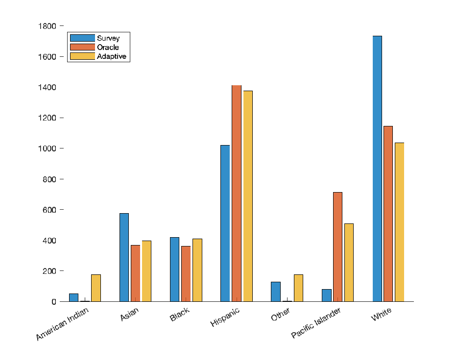
We propose to use our sampling strategy for tracking SARS-CoV-2 seroprevalence in populations classified on the basis of location, ethnicity, age etc. Each category of interest can be modeled as an arm with a Bernoulli pmf, where the probability represents the positivity associated with category . We use data from a randomized seroprevalence survey conducted in Los Angeles county Sood et al. 2020. The plots in Figures 2 and 2 depict the gap between optimal sample allocation and the random allocation strategy used by the survey. This gap illustrates the importance of adaptive randomized sampling for obtaining uniform estimates of seroprevalence. Without careful sampling, we can have bad estimates for certain groups that may be particularly vulnerable.
[][t] \subfigure[][t]
Remark 8.
For estimating SARS-CoV-2 seroprevalence, there are some practical aspects that require a slightly different formulation and sampling strategy. We provide a heuristic approach for addressing these issues and the analysis of this approach is a problem for future work.
6 Conclusions and Future Work
For the problem of uniformly estimating pmfs in a mean squared sense, a UCB sampling approach is proposed. Unlike the state-of-the-art approach in Shekhar et al. 2020, a Dirichlet prior is assumed on the pmfs and the upper confidence bounds are computed based on the posterior. It is analytically shown that the performance of this Bayesian approach can be now worse than the approach in Shekhar et al. 2020, and has noticeably better performance in practice. We discuss the potential application of the sampling approach for SARS-CoV-2 seroprevalence and incidence rate estimation.
There are two potential directions for future work. One is to incorporate temporal variation in the underlying pmfs. This is particularly important in studying SARS-CoV-2 incidence rates. The other is to incorporate a prior on the collection pmfs so that the correlation between them can be exploited to improve our estimates and the sampling strategy. For both these directions, a Bayesian model can be more helpful.
Appendix A Proof of Lemma 5
A Beta distribution with parameters is sub-Gaussian with parameter Marchal et al. 2017. And because of (10) we can conclude using the Chernoff bound Ross 2014 that
| (20) | ||||
| (21) |
Since and are selected using the inverse cdf of the posterior distribution, we have
| (22) |
The second inequality in the lemma simply follows from the fact the .
Appendix B Proof of Lemma 6
Under event , we have
| (23) | ||||
| (24) | ||||
| (25) | ||||
| (26) | ||||
| (27) | ||||
| (28) | ||||
| (29) |
Here, inequality in is because of the triangle inequality and the inequality in is due to Lemma 5.
Appendix C Proof of Theorem 4
We have
| (30) | ||||
| (31) | ||||
| (32) |
where . Note that the last equality in the display above follows from a simple change of measure argument. Since is the probability of the unfavorable event conditioned on the model , we can obtain a regret bound in terms of without local averaging using the same arguments as in the proofs of Lemma 1 and Theorem 1 in (Shekhar et al. 2020, Appendix D.3). Thus, we have
| (33) | ||||
| (34) |
where
| (35) | ||||
| (36) | ||||
| (37) |
and . Using (32), we can then locally average the regret as
| (38) | ||||
| (39) | ||||
| (40) |
Appendix D Incorporating Priors
In this section, we will consider a scenario where we are provided with a prior on . We will first modify the distribution used for local averaging as
| (41) |
for any Borel measurable set . Here, is a ball around with .
Dirichlet priors
When the prior is any factored Dirichlet distribution (i.e. not necessarily uniform) of the form in (8), one can easily extend all the results with the modified .
Intervals for Bernoulli parameters
Another scenario of interest is when and we are given that the Bernoulli parameter associated with lies in some interval . We can then assume that the Bernoulli parameter is distributed uniformly and independently over the interval . Since this prior does not correspond to a Beta distribution, the posterior belief may not be a Beta distribution. However, we still can easily find the cdf of the posteriors in this case because the posterior on the parameters is just going to be a truncated Beta distribution. Let be the cdf of the posterior at time with a uniform prior and let be the posterior with the truncated prior. Then one can show that
| (42) |
The confidence intervals in (12) and (13) can then be computed using the inverse of .
Appendix E Practical Considerations: Overall Estimate and Batch Sampling
In seroprevalence estimation, we generally allocate samples in batches of size . Also, we are generally interested in estimating the positivity of each category as well as the positivity in the overall population. Let the fraction of individuals of category in the overall population be . Then the overall positivity and its estimate are given by
| (43) | ||||
| (44) |
The mean squared error between and is given by
| (45) |
If the mean squared error associated with is not considered, then it may so happen that a tiny group (small ) with high positivity will be allocated too many samples. The contribution of this small group to the overall estimate would be small and thus, allocating too many samples to it could compromise the quality of the overall estimate . Therefore, we need to determine an allocation that accounts for the quality of the overall estimate as well.
A suitable way to formalize this notion is to pose the following constraints on the oracle allocation
| (C1) | ||||
| (46) | ||||
| (47) | ||||
| (48) |
where , are predetermined constants. A solution to the above set of constraints can be obtained by solving the following optimization problem
| (C2) | ||||
| (49) | ||||
| (50) |
The Problem (C1) is feasible if and only if the optimum value of the optimization problem above is less than or equal to 1. In that case, the solution to Problem (C2) is a solution to Problem (C1). Notice that Problem (C1) is very similar to Problem (P1) except for the additional mean squared error term associated with the overall estimate . Because of this distinction, it is not clear whether one can view Problem (C2) as a particular instance of Problem (P1) with appropriate modifications and simply apply the adaptive sampling strategy in Section 4 to the modified problem. Nonetheless, we provide a similar heuristic sampling approach that tracks the oracle quite well (See Figure 3). At each time time , the heuristic is to allocate samples within each batch according to the solution of the following optimization problem
| (C3) | ||||
| (51) | ||||
| (52) | ||||
| (53) | ||||
| (54) |
acknowledgments-disclosure-of-funding.
This research was supported, in part, by National Science Foundation under Grant NSF CCF-1817200, CCF-1718560, CPS-1446901, Grant ONR N00014-15-1-2550, and Grant ARO W911NF1910269.References
- Bayarri and Berger (2004) M Jésus Bayarri and James O Berger. The interplay of bayesian and frequentist analysis. Statistical Science, pages 58–80, 2004.
- Brown et al. (2001) Lawrence D Brown, T Tony Cai, and Anirban DasGupta. Interval estimation for a binomial proportion. Statistical science, pages 101–117, 2001.
- Carpentier et al. (2011) Alexandra Carpentier, Alessandro Lazaric, Mohammad Ghavamzadeh, Rémi Munos, and Peter Auer. Upper-confidence-bound algorithms for active learning in multi-armed bandits. In International Conference on Algorithmic Learning Theory, pages 189–203. Springer, 2011.
- Efroni et al. (2020) Yonathan Efroni, Shie Mannor, and Matteo Pirotta. Exploration-exploitation in constrained mdps. arXiv preprint arXiv:2003.02189, 2020.
- Kotz et al. (2004) Samuel Kotz, Narayanaswamy Balakrishnan, and Norman L Johnson. Continuous multivariate distributions, Volume 1: Models and applications. John Wiley & Sons, 2004.
- Marchal et al. (2017) Olivier Marchal, Julyan Arbel, et al. On the sub-gaussianity of the beta and dirichlet distributions. Electronic Communications in Probability, 22, 2017.
- Rosenberg and Mansour (2019) Aviv Rosenberg and Yishay Mansour. Online convex optimization in adversarial markov decision processes. In International Conference on Machine Learning, pages 5478–5486, 2019.
- Ross (2014) Sheldon M Ross. Introduction to probability models. Academic press, 2014.
- Shekhar et al. (2020) Shubhanshu Shekhar, Mohammad Ghavamzadeh, and Tara Javidi. Adaptive sampling for estimating probability distributions. In International Conference on Machine Learning, 2020.
- Sood et al. (2020) Neeraj Sood, Paul Simon, Peggy Ebner, Daniel Eichner, Jeffrey Reynolds, Eran Bendavid, and Jay Bhattacharya. Seroprevalence of sars-cov-2–specific antibodies among adults in los angeles county, california, on april 10-11, 2020. Jama, 2020.
- Tarbouriech and Lazaric (2019) Jean Tarbouriech and Alessandro Lazaric. Active exploration in markov decision processes. In The 22nd International Conference on Artificial Intelligence and Statistics, pages 974–982, 2019.