Plane Wave Elastography: A Frequency-Domain Ultrasound Shear Wave Elastography Approach
Abstract
In this paper, we propose Plane Wave Elastography (PWE), a novel ultrasound shear wave elastography (SWE) approach. Currently, commercial methods for SWE rely on directional filtering based on the prior knowledge of the wave propagation direction, to remove complicated wave patterns formed due to reflection and refraction. The result is a set of decomposed directional waves that are separately analyzed to construct shear modulus fields that are then combined through compounding. Instead, PWE relies on a rigorous representation of the wave propagation using the frequency-domain scalar wave equation to automatically select appropriate propagation directions and simultaneously reconstruct shear modulus fields. Specifically, assuming a homogeneous, isotropic, incompressible, linear-elastic medium, we represent the solution of the wave equation using a linear combination of plane waves propagating in arbitrary directions. Given this closed-form solution, we formulate the SWE problem as a nonlinear least-squares optimization problem which can be solved very efficiently. Through numerous phantom studies, we show that PWE can handle complicated waveforms without prior filtering and is competitive with state-of-the-art that requires prior filtering based on the knowledge of propagation directions.
December 2020, Patent Pending.
Keywords: Ultrasound shear wave elastography (SWE), frequency-domain, scalar wave equation, plane wave, soft tissue, cancer diagnosis, lesion, phantom.
1 Introduction
Soft tissue pathology is known to be correlated with change in tissue stiffness [WGRCUE2015SNPH]. For instance, an increase in cellular density caused by malignant tumors, leads to an increased tissue stiffness [CPUSEETN2014MSMF, SWEBVQC2015BZ, ESWECFLL2017GFSW]. Ultrasound elastography methods utilize this correlation by mechanically exciting the tissue and analyzing the subsequent motion to quantify its stiffness over a region of interest (ROI). Various clinical studies of such methods indicate their relevance for non-invasive monitoring and diagnosis of breast and liver diseases among others [BLQESSI2010ATTS, USRTCA2017SLEC]. In the case of breast cancer for instance, ? used the quantitative ratio of lesion to background stiffness to determine the probability of malignancy, with higher contrasts indicating higher probability of the lesion being malignant.
Different ultrasound elastography techniques exist in the literature that can broadly be categorized into strain imaging and shear wave elastograohy (SWE) methods [USRTCA2017SLEC]. Particularly, SWE methods generate and track shear waves that travel in the tissue with wave-speeds considerably smaller than their compressional counterparts (typically below m/s) and have a low frequency content (below Hz). In these methods, the tissue excitation is achieved by a vertical displacement ( µm) using an acoustic radiation force (ARF) impulse from an ultrasound push beam, while high frame-rate ultrasound imaging techniques are used to track the induced shear wave [USWEISDP2016DRPN]. The supersonic shear imaging (SSI) method proposed by ?, is one of the early works to outline the SWE approach and demonstrate its performance. On the other hand, the comb-push ultrasound shear elastography (CUSE) of ?, is a more recent work that relies on simultaneous, parallel ARF beams and compounding to improve the quality of shear modulus11 1 Shear modulus is one of the several quantities used to measure the stiffness of materials.estimations.
A number of different SWE algorithms have been proposed to estimate the shear modulus field from wave data. For instance, ? utilized the scalar wave equation along with the Fourier-transformed second-order derivatives of the scalar displacement field, while ? proposed the use of a level-set function of wave-front arrival time. However, most currently used SWE methods, including the commercialized versions of SSI [BLQESSI2010ATTS] and CUSE [CUSEBMIR2015DMSM] systems, utilize the time-of-flight (ToF) technique to estimate the wave-speed and corresponding shear modulus field [QABLV2008TBAD, QHSMVARF2008PWDF, PARAQSWI2012RWPN, CPUSE2012SZMU, FSCSWSC2014SMZU, ISWGVEMSPTM2017CCMGU]. For instance, [QABLV2008TBAD, FSCSWSC2014SMZU] utilize cross-correlation of the signal at nearby locations along the propagation direction (typically the lateral axis) to estimate the ToF, i.e., the time that it takes the wave-front to reach the second point from the first point. Alternatively, the time-to-peak of shear waveform can also be used to estimate the time-of-flight [QHSMVARF2008PWDF, PARAQSWI2012RWPN, ISWGVEMSPTM2017CCMGU]. These methods assume that the medium is locally homogeneous, isotropic, incompressible, and linear-elastic [GFEMARFSW2016PQSU] and rely on the prior knowledge of the propagation direction which is assumed to be perpendicular to the ARF push axis [USWEISDP2016DRPN]. This assumption is reasonable for ‘directional’ shear waves with flat wave-fronts; see [USRTCA2017SLEC] for details. We define a directional shear wave as a wave that has a clear dominant propagation direction.
In the presence of inhomogeneities like tumors, shear waves scatter due to reflection and refraction, violating the directionality assumption of ToF methods, which can lead to artifacts in the estimated shear modulus field [ERWTSWE2011DGBT, RSWFETP2017POZC]. Directional filters are then necessary to remove the reflections and obtain directional waves [SDFIIMR2003MLKE, ERWTSWE2011DGBT, EISWSEMDF2016LRPN]. In their simplest form, directional filters are frequency-domain projections that only retain the wave components aligned with the given propagation direction; see [ERWTSWE2011DGBT] for details. They decompose the shear wave into a set of directional waves that can be separately analyzed via the ToF method. In addition to reflection and refraction, noise in the wave data can create artifacts in the estimated fields and a second radial filter is often necessary to improve the signal-to-noise ratio; see A for details. Ultimately, the shear modulus fields corresponding to different directions are combined through compounding (averaging) to obtain a final shear modulus field. When the direction of propagation is not aligned with the lateral axis, one dimensional (1D) analysis can overestimate the wave-speed. The fast shear compounding (FSC) method proposed by ? utilizes a 2D analysis of wave-speed along with prior filtering for robust shear modulus estimation in inhomogeneous mediums. It extends the CUSE method [CPUSE2012SZMU] to include multiple simultaneous ARF beams with arbitrary known directions. In Section 4, we compare our proposed approach to this method.
Another set of SWE methods exist that rely on similar assumptions but perform the wave-speed (phase velocity) analysis in the frequency domain [QEVMSWS2004CFG, SDUVMTE2009CUPK, DCSLMIURF2016BBBDT, VMILSWD2017VWWM, LPVI2018KU]. For instance, the local phase velocity imaging method proposed by ?, relies on short space 2D Fourier transform analysis of the wave data to extract the most dominant wavenumber within a homogeneous window. Assuming a directional propagation within the window, the phase velocity is estimated as the ratio of angular frequency to wavenumber. As discussed earlier, the assumption of directional propagation breaks down in the presence of inhomogeneities. Another family of frequency-domain methods utilize the elastodynamic partial differential equation (PDE) to rigorously model the shear wave propagation in this general form, automatically accounting for reflection and refraction. These methods can be classified into direct [SMRDETHC2006PM] and iterative [VCSTDFEM2008ESRO, MECEUE2017GZBA, AECETE2019AB] approaches. Direct methods, although more efficient, are sensitive to noise. The iterative methods on the other hand, despite versatility, are computationally demanding which has limited their practical utility.
It is known that for shear waves induced by ARF beams, the displacement component parallel to the push axis is dominant [GFEMARFSW2016PQSU]. Thus, we can use a scalar wave equation, instead of the elastodynamic PDE, to capture only the dominant shear wave component. Relying on this observation, we develop a novel frequency-domain SWE approach, called Plane Wave Elastography (PWE), that does not require the prior knowledge of propagation direction and is considerably more computationally efficient than the PDE-constrained approaches. More specifically, given a homogeneous subdomain within the ROI, we represent the solution of the scalar wave equation as a linear combination of plane waves with arbitrary propagation directions. Using this representation, we formulate the SWE problem as a nonlinear least-squares problem that can be efficiently solved for the constant wave-speed within the subdomain. The PWE method relaxes the need for prior denoising by relying on a regularized least-squares formulation and directional filtering through automatic selection of dominant plane waves and does not require the post-processing step of compounding. Moreover, the optimal mean squared error (MSE) is an indicator of how closely the data conforms to the scalar wave equation. This can be used to provide feedback on the quality of reconstruction since higher levels of MSE indicate deviation from the wave model due possibly to noise. Finally, when the geometry of inclusions is known, e.g., from B-mode images, the PWE method can reconstruct the shear modulus field by a single solve for each homogeneous subdomain.
In summary, compared to the common SWE methods, our approach (i) has competitive reconstruction performance without relying on prior denoising, directional filtering and the prior knowledge of the propagation direction, or the need for compounding, (ii) provides feedback on quality of reconstructions using the MSE, and (iii) can take advantage of the prior knowledge of the inclusion geometry, if available, to speed up computations and improve the estimation contrast.
A closely related approach to PWE was proposed by ? for magnetic resonance elastography (MRE). In their approach, the solution of an elastodynamics PDE was approximated using a set of plane wave expansions in a similar vein as in our PWE approach. However, their work considers a vector-valued problem in which all components of displacements are required. This is not directly applicable to an ultrasound modality where only one component of displacement is usually available. Our approach improves upon this previously proposed method in several key aspects by: i) adapting the plane-wave expansion to the scalar wave equation, thus enabling the use of ultrasound tracking, ii) decreasing the ensuing computational cost, iii) adding a multi-frequency treatment and, iv) incorporating the systematic and consistent treatment of noise through regularization which enables more accurate reconstructions without prior filtering. A comparison of the approach proposed by ? to other popular MRE techniques is given by ?. Finally, ? also utilized a plane-wave expansion, but to model narrow-band reverberant wave fields in which, no propagation direction is dominant. This does not apply to the ARF-based SWE problem considered here which often has a few dominant directions.
The remainder of this paper is organized as follows. In Section 2, we formulate the SWE problem and in Section 3, we present the PWE approach to solve it. In Section 4, we present various phantom studies demonstrating the performance of the PWE method. Section 5 is dedicated to discussing various aspects of our method highlighting its strengths and weaknesses, and Section 6 concludes the paper.
2 Problem Formulation
2.1 Scalar Wave Equation
Let denote the region of interest (ROI) and consider a shear wave propagating in in response to one or a set of acoustic radiation force (ARF) push beams applied outside ; let denote the in-plane displacement at time and point due to this shear wave. Ultrasound transducers often only measure the dominant component of the displacement parallel to the push directions; let denote this dominant component.
Assuming that the medium is isotropic, incompressible, and linear-elastic [GFEMARFSW2016PQSU], and assuming that the ARF push beams are applied outside the ROI, we can represent the propagation of the shear wave in using the scalar wave equation
where kg/m3 is the mass density of the soft tissue and is the shear modulus field; denotes the positive real numbers. Note that the shear modulus is related to the shear wave-speed as
| (1) |
Let denote the Fourier transformed signal with respect to the temporal coordinate at a frequency , i.e., . Then, given frequency , the scalar wave equation can be written in the frequency-domain as
| (2) |
Consider a homogeneous subdomain with constant shear modulus . Then, we can write solutions to the scalar wave equation (2) in as a linear combination of basis functions , i.e.,
| (3) |
where is the number of basis functions, , and the basis functions are plane waves explicitly given by
| (4) |
In this expression, denotes the unit imaginary number, is the constant wave-speed within the homogeneous subdomain , and are unit direction vectors of propagation, i.e., , where denotes the Euclidean -norm. Fig. 1 depicts a plane wave of form (4) and a shear wave obtained by superposing plane wave bases according to (3).


2.2 Shear Wave Elastography Problem
Let denote the temporal signal measured at points for and denote the corresponding (discrete) Fourier transformed signal at a frequency . The objective of the elastography problem then is to find the constant shear modulus or equivalently the wave-speed within the homogeneous subdomain . Given the basis expansion (3), we can formulate this problem as a nonlinear least-squares optimization problem as follows:
| (5) |
where is the vector of coefficients and is the design matrix with
| (6) |
for .
Whenever the number of measurements is less than the number of bases , the optimization problem (5) is ill-posed. Furthermore, often the measured signal is contaminated with noise and we do not want the solution (3) of the wave equation (2) to perfectly match the measurements . To address these challenges, we add a regularization term to (5) that improves stability and allows us to control how closely we fit the data:
where is the regularization parameter. Note that the use of regularization encourages selection of a subset of plane waves and helps distinguish dominant propagation directions by penalizing nonzero coefficients .
So far we have utilized the data at a single frequency . It is often necessary to consider a set of dominant frequencies , where denotes the number of frequencies. Given measurements for , we use the linear expansion (3) with coefficients to represent the solution of the scalar wave equation (2) at frequency . Then, the corresponding elastography problem is given by
| (7) |
Shear wave data are often calculated from the in-phase-quadrature data using an autocorrelation algorithm [RTBFIAT1985KNKO] and are given as particle velocity and not displacement. Noting that , we can represent the (discrete) Fourier transformed velocity data with an expansion similar to (3) and scaled coefficients. Therefore, regardless of whether displacement or velocity data are used, the elastography problem is formulated as (7). In the next section, we discuss an efficient approach to solve this optimization problem.
3 Plane Wave Elastography
3.1 Solution to the Elastography Problem in a Homogeneous Subdomain
Solving the optimization problem (7) can be challenging due to nonlinearity; see B. However, for a fixed wave-speed , (7) is a standard -regularized least-squares problem whose solution for each frequency, is given in closed-form by
| (8) |
where is the identity matrix and the superscript denotes the conjugate transpose operator. Given this closed-form expression and since within the homogeneous subdomain , the wave-speed is a constant scalar, we can utilize a global search algorithm or a simple discretization method to find the optimal wave-speed as
| (9) |
where are the lower-bound and upper-bound on the wave-speed and is the optimal regularized least-squares solution (8) for a given wave-speed .
Assume that we use a limited number of basis functions and frequencies along with appropriate regularization to prevent overfitting the noise. Then, the value of the least-squares term corresponding to the optimal wave-speed can be used as a measure of conformity of the data to the scalar wave equation (2); the smaller the least-squares error, the closer the data is to the underlying physics. Thus, we can use this feedback to evaluate the quality of reconstruction. Particularly, we use the mean squared error (MSE), given by
| (10) |
as a measure of the quality of reconstruction in .
3.2 Plane Wave Elastography Algorithm
Our solution in Section 3.1 was for a homogeneous subdomain with constant shear modulus. To estimate the shear modulus field over an inhomogeneous ROI, we discretize the ROI into grid points and use windows of size with constant shear moduli. Particularly, for a point we define a window (subdomain) as
| (11) |
We solve (9) to estimate the wave-speed and the corresponding shear modulus within and assign the value to point , constructing in this way, a discretized vector of estimations for the shear modulus field ; see Fig. 2.
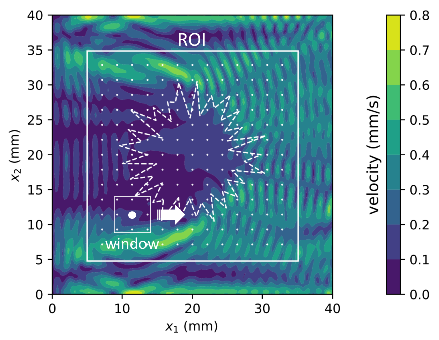
The Plane Wave Elastography (PWE) approach is summarized in Algorithm 1.
The algorithm starts by requiring the discretization points and window size , as well as the number of plane wave basis functions and dominant frequencies . In line 2, given the (discrete) Fourier transformed displacement signal , it selects the regularization parameter ; see Section 3.3 for details. Then, the algorithm loops over the discrete points within the ROI. In line 4, given the measurements within window for , it extracts the dominant frequencies contributing the highest amount of energy to the Fourier spectrum, and the corresponding measurements for . Then, in line 5, it computes the constant wave-speed for window from (9) and the corresponding MSE from (10). In line 7, collects the estimated shear moduli corresponding to all discretization points within the ROI. Given , we can approximate the shear modulus field at any point via interpolation.
3.3 Parameter Selection
Next, we discuss the important parameters that affect the performance of the PWE Algorithm 1. As discussed in Section 1, an important advantage of the PWE approach is that it does not rely on the directionality of the propagation, due to the plane wave representation in (3). In the absence of any prior knowledge on the directionality of the propagation, we choose the directions to uniformly sample , i.e.,
| (12) |
As we demonstrate in Section 4, in practice often directions are sufficient to resolve the propagating waves.
An important parameter for the PWE method is the number of dominant frequencies . In principle, increasing adds more information and leads to more accurate reconstructions. However, one should take caution not to include very high frequencies with unfavorable signal to noise ratios, i.e., must be upper-bounded, where is the corresponding frequency in Hertz. Another important parameter is the lower-bound on dominant frequencies, which determines the longest wavelength in the data. More specifically, where is the unknown maximum wave-speed in the ROI. As a general rule of thumb, for data with a high signal-to-noise ratio (SNR), the window size must be larger than to ensure that waves can be resolved with a window of size . Note that also determines the number of measurements used to estimate the wave-speed in each subdomain . Using at least measurements is required to ensure that the design matrix (6) is well-conditioned. When the SNR is low, larger values of should be used to ensure that the measurements contain adequate information about the unknown wave speed. In practice, the range of dominant frequencies and the spatial resolution of measurements are fixed for a given shear wave data but both and SNR are unknown. As a result, for best reconstructions we might need to adjust . The quality of reconstructions by the PWE Algorithm 1 are often better for data with higher SNR and for which smaller values of can be used.
When data is noisy, a major parameter that affects the reconstruction is the regularization parameter . As discussed in Section 2.2, proper selection of allows us to simultaneously perform filtering and reconstruction. In this paper, we utilize the L-curve approach to select . This involves plotting the regularization term in (9) versus the sum-of-squares value (a constant multiple of MSE (10)) as a function of and selecting the regularization parameter corresponding to the point of maximum curvature in the L-curve;22 2 Due to the extra minimization with respect to wave-speed in (7), the curve generated in this way is not exactly the L-curve but as we show in Section 4, this version can still be used to select appropriate regularization parameters.see [DIP2010H]. In Section 4.4, we present parameter study results to further clarify the discussion of this section.
3.4 Prior Knowledge of ROI Geometry
In practice, the prior knowledge of the location and shape of inclusions (inhomogeneities) within the ROI might be available, e.g., from B-mode images. In that case, we can estimate the shear modulus field with a considerably fewer solves than what is needed in Algorithm 1, which requires one solution per discretization point. Particularly, consider a decomposition of the ROI into non-overlapping subdomains such that where within the shear modulus is constant and equal to . Then, solving (9) with measurements belonging to , we obtain an estimate of the wave-speed and the corresponding shear modulus from (1) and we can estimate the shear modulus field as
| (13) |
where the indicator function and is zero otherwise.
4 Experiments
In this section, we present phantom studies to demonstrate the performance of the PWE Algorithm 1. Particularly, we first study a digital phantom with a complex inclusion mimicking a malignant tumor to induce reflections and refractions, demonstrating the ability of PWE to resolve complicated wave patterns without prior filtering. Then, we consider two categories of phantom experiments. The first category involves four simultaneous ARF push beams applied using a curved-array ultrasound transducer at different angles and validates in practice, the ability of the PWE approach to resolve waves traveling at unknown arbitrary directions. We also consider the more common case of two parallel push beams generated by a linear transducer. For these phantom experiments, we calculate the shear wave data from the in-phase-quadrature data using an autocorrelation algorithm [RTBFIAT1985KNKO]. Finally, we study the effect of various parameters on the performance of PWE to further illustrate the discussion of Section 3.3.
In each case, in addition to nominal values, we report reconstructions by the fast shear compounding (FSC) method, proposed by ?, to validate the PWE reconstructions and demonstrate that PWE performs at least as well as the state-of-the-art33 3 FSC method is commercially used on General Electric LOGIQ E9 SWE system [TSWECU2015SMBL]., even though it does not require prior filtering or post-processing. Note that the FSC method strongly relies on directional filtering to ensure the directionality of the waves and radial filtering in the spatial frequency domain, to enhance the SNR; see A for details. In the case of a multi-push excitation, the FSC method reconstructs shear modulus fields individually for each filtered direction and then uses compounding to combine the reconstructions. In the following, we fine-tune the parameters of this method for best possible reconstructions. We particularly report the window size defined similar to (11), and the patch size which is the distance between pairs of points used for cross-correlation to determine the time-of-flight; see [FSCSWSC2014SMZU] for details.
To measure the reconstruction performance, we report the average shear moduli over the background and inclusion along with the standard deviations , where denote the estimated shear modulus vector confined to subdomains , respectively. We also report the contrast-to-noise ratio (CNR), defined as
| (14) |
Throughout this section, for PWE reconstructions we use dominant frequencies and basis functions and set the maximum frequency to Hz; see Section 4.4 for the reasoning behind this selection. We also set the wave-speed bounds in (9) to m/s and m/s, which is a reasonable range for soft tissue. Moreover, to conform to the ultrasound coordinate system convention, where the transducer is located on top, in the following plots we use axial or depth axis and lateral axis with the origin located on the top-left corner.
4.1 Single-push Digital Phantom
In this section, we study the performance of PWE for a mm mm digital phantom with an inclusion mimicking a malignant tumor, see e.g. [CPSMMLSB2016LWXL, Fig. 1], with a background shear modulus of kPa and inclusion shear modulus of kPa; see Fig. 3 for the shape of the inclusion. To simulate the shear wave propagation, we discretize the domain with a spatial interval of µm and temporal step-size of µs and solve the 2D incompressible elastodynamic PDE [AECETE2019AB] in FEniCS [alnaes2015fenics] using a mixed finite element method, subject to an unfocused ARF impulse modeled by a sinusoidal traction with frequency of Hz along the right side of the domain. The duration of the impulse was and the duration of the simulation was ms. In the following, we study the performance of PWE without and with noise over a mm mm ROI.
The plots in the first row of Fig. 3 show the reconstructions for noiseless data.
| (a) FSC | (b) PWE | (c) MSE | (d) cross-section | |
|---|---|---|---|---|
|
noiseless data |
 |
|||
|
noisy data |
For PWE results, we set the minimum frequency to Hz after inspecting the Fourier transfer spectrum, and the window size to mm, accordingly. Because the data is noiseless, a wide range of values are appropriate for the regularization parameter; we set from the L-curve analysis. From the PWE reconstruction, the average background and inclusion shear moduli are kPa and kPa, respectively. The contrast-to-noise ratio is CNR dB. Referring to the MSE field in column (c) of Fig. 3, observe that the regions at the boundary of inclusion and background have the highest MSE values (10) since at those regions, the assumption of homogeneity breaks down (the windows cover parts of both the inclusion and background). Moreover, generally the MSE values are smaller inside the inclusion indicating better agreement with the wave equation (2). For the FSC method [FSCSWSC2014SMZU], we get kPa and kPa and CNR dB, where we use a window size of mm and patch size of mm. Referring to cross-section plots in column (d) of Fig. 3, observe that the inclusion edges are smoothed out due to windowing, resulting in slightly skewed estimations compared to the ground truth.
To investigate the effect of noise, we contaminated the simulated data with additive Gaussian noise decreasing the signal-to-noise ratio to SNR dB.44 4 Although Gaussian noise is not an accurate model of the ultrasound noise, it has been used in the literature regardless; see e.g., [RPVDEVM2018KQC]. In the next sections, we study phantom experiments that inherently contain realistic ultrasound noise. The plots in the second row of Fig. 3 show the reconstructions for this case. In the presence of noise, more measurements are required for the same minimum frequency Hz, to ensure reasonable reconstructions. Using mm and from the L-curve analysis, we get kPa and kPa, and CNR dB from the PWE method. Referring to the MSE feedback in column (c), we can see that the MSE values are orders of magnitude higher in this case indicating considerable disagreement with the wave equation (2). Because the noise is uniformly added across all spatial locations, the MSE values are very close throughout the ROI. Finally using the FSC method, we get kPa and kPa and CNR dB, where we use a window size of 2.00 mm and patch size of 1.75 mm. Note that prior filtering to improve the SNR is essential to obtaining reasonable reconstructions using the FSC method in the presence of noise.
4.2 Multi-push CIRS Phantom
Next, we consider a phantom with nominal background shear modulus of kPa and a single spherical inclusion with shear modulus of kPa and diameter of mm (Model 049, CIRS, Inc., Norfolk, VA), excited by four simultaneous ARF push beams transmitted by a C5-2 curved-array transducer (Verasonics, Inc., Kirkland, WA) and measured with a research scanner (V1, Verasonics, Inc., Kirkland, WA). Each push beam used elements, and the beams were moved to the edge of the transducer such that two beams were formed on the extreme left and right sides of the array and elements in the center were inactive. We study two ARF push configurations with push frequency of MHz: (i) one push with duration of µs; (ii) four repeated pushes of duration µs separated by µs of waiting, generating a repeated push of Hz. This repeated push is intended to excite a wider frequency range [HPEMD2008UG]. A movie of the vertical shear wave velocity component generated under these two push configurations can be found in [meJ6_video1]. Fig. 4 depicts the geometry of the phantom and the mm mm ROI along with the approximate location of the inclusion and the focused push beams (focal depth is mm).

Note that the prior knowledge of the push beam angles and equivalently the propagation directions, is not required for PWE. The spatial spacing of the shear wave data was µm while the temporal interval was µs. The duration of the signal was ms.
The plots in the first row of Fig. 5 depict the reconstructions for the push configuration (i).
| (a) FSC | (b) PWE | (c) MSE | (d) cross-section | |
|---|---|---|---|---|
|
push config. (i) |
 |
|||
|
push config. (ii) |
For the PWE results in column (b), we use Hz and µm and set as before. Note that basis functions are sufficient to reconstruct the field even though the PWE Algorithm 1 is unaware of the propagation directions. We use a regularization parameter of , obtained from the L-curve in Fig. 6; see Section 3.3 for details.

The average shear moduli are kPa and kPa and the contrast-to-noise ratio (14) is CNR dB. Given the prior knowledge of inclusion geometry from the B-mode image in Fig. 4, we get more accurate estimates kPa and kPa, where we use settings similar to the previous reconstruction and set from the L-curve analysis; see Section 3.4 for details.
The contour plot in column (a) of Fig. 5 shows the corresponding FSC reconstruction for push configuration (i). To obtain the FSC estimate, using directional filters we decompose the shear wave into four directional waves traveling along angles and rely on a radial filter to enhance the SNR. We use window and patch sizes of mm and mm, respectively. After constructing the shear modulus estimates for the individual waves, we combine them using compounding; see [FSCSWSC2014SMZU] for details. The average shear moduli in this case are kPa and kPa and the contrast-to-noise ratio (14) is CNR dB. We also performed a reconstruction given the prior knowledge of the geometry, where we average the values from windows that completely fall within the background or inclusion. Using a similar window size, we get the improved estimates kPa and kPa.
The plots in the second row of Fig. 5 depict the reconstructions for push configuration (ii). This ARF configuration results in a wider frequency range at the expense of lower SNR which requires larger window sizes for acceptable reconstructions. For PWE, we use Hz and mm and from Fig. 6, resulting in kPa and kPa and CNR dB. Relying on the prior knowledge of inclusion geometry and with obtained from the L-curve analysis, we get kPa and kPa. It can be seen that using the prior knowledge improves the estimation inside the inclusion but deteriorates it for the background. This is due to the fact that parts of the background have higher noise levels and solving the SWE problem (7) only once, lumps all measurements into a single estimate. In practice it might be beneficial to decompose the background into multiple subdomains.
Plots in column (c) of Fig. 5 show the MSE (10) feedback from the PWE method for the two ARF configurations. Note the higher variations in background MSE values for both cases. Note also that the values for configuration (ii) are an order of magnitude higher indicating further inconsistency with the physics of the wave propagation. This lower SNR is also evident from Fig. 6 where the L-curve for configuration (ii) is shifted to the right (higher sum of squares).
Finally, column (a) in the second row of Fig. 5 shows the FSC reconstruction where we perform similar filtering procedures to decompose the wave and improve the SNR. With window and patch sizes of mm and mm, we get kPa and kPa and CNR dB. Relying on the prior knowledge of the geometry and with window and patch sizes of mm and mm, we get kPa and kPa. It seems that in this specific case, the performance of the FSC method degrades more with noise than the PWE method; similar behavior was observed for other data with similar push configuration. Table 1 summarizes the estimated shear modulus values for the reconstructions of this section. Note that PWE reconstructions are generally more accurate.
| method | push configuration (i) | push configuration (ii) | ||||
| (kPa) | (kPa) | CNR (dB) | (kPa) | (kPa) | CNR (dB) | |
| PWE | ||||||
| FSC | ||||||
| PWE with prior | - | - | ||||
| FSC with prior | - | - | ||||
4.3 Parallel Double-push CIRS Phantoms
In this section, we consider phantoms with two parallel ARF pushes applied using a Verasonics V1 system with a L7-4 transducer (Philips Healthcare, Andover, MA) on the sides of the phantom at mm focal depth. Specifically, we consider a homogeneous phantom with nominal background shear modulus of kPa (Model 039, CIRS, Inc., Norfolk, VA), a soft Type I cylindrical inclusion with diameter mm and nominal shear modulus of kPa, and three stiff Type IV cylindrical inclusions with diameters mm, mm, and mm and nominal shear modulus of kPa (Model 049A, CIRS, Inc., Norfolk, VA). The push duration was µs and the push frequency was MHz. The push beams were generated by active elements located at the edges of L7-4 probe. Fig. 7 shows the B-mode image for the phantom with inclusion size of mm along with the position of the push beams and the mm mm ROI.

The spatial spacing of the shear wave data was µm while the temporal intervals were µs and µs for the homogeneous phantom and with inclusions, respectively. The duration of the signal was ms in all cases.
Fig. 8 shows the reconstructions for both PWE and FSC methods over a mm mm ROI without and with the prior knowledge of inclusion geometry, while Table 2 reports the corresponding average shear moduli and CNR values (14).
| (a) FSC | (b) PWE | (c) MSE | (d) cross-section | |
|---|---|---|---|---|
|
homogeneous |
||||
|
soft inclusion |
||||
|
10.40 mm |
 |
|||
|
6.49 mm |
||||
|
4.05 mm |
| method | homogeneous | soft inclusion ( mm) | stiff inclusion ( mm) | ||||
| CNR | CNR | ||||||
| (kPa) | (kPa) | (kPa) | (dB) | (kPa) | (kPa) | (dB) | |
| PWE | |||||||
| FSC | |||||||
| PWE with prior | - | - | |||||
| FSC with prior | - | - | |||||
| method | - | stiff inclusion ( mm) | stiff inclusion ( mm) | ||||
| - | CNR | CNR | |||||
| - | (kPa) | (kPa) | (dB) | (kPa) | (kPa) | (dB) | |
| PWE | - | ||||||
| FSC | - | ||||||
| PWE with prior | - | - | - | ||||
| FSC with prior | - | - | - | ||||
For the PWE reconstructions, by inspecting the Fourier spectrums, for all cases except for the soft inclusion, we set the minimum frequency to Hz, for the soft inclusion we set Hz, and the window size to mm in all cases. In each case, the regularization parameter is selected according to an L-curve similar to Fig. 6; see Table 3 for numerical values.
| inclusion type | without prior | with prior |
|---|---|---|
| homogeneous | ||
| soft inclusion ( mm) | ||
| stiff inclusion ( mm) | ||
| stiff inclusion ( mm ) | ||
| stiff inclusion ( mm) |
For the FSC method, we use window and patch sizes of mm and mm, respectively. Note that as in the previous cases, the PWE method is unaware of the directions of propagation. Nevertheless, the PWE reconstructions without prior directional filtering are competitive with the FSC method and often more accurate. For the homogeneous case in the first row of Fig. 8, the estimates are not in agreement with the nominal values due possibly to the change in mechanical properties of the phantom over time55 5 The homogeneous phantom was manufactured before April 12, 2014 and is over six years old. [TWEMFAIP2011BSHS] but the PWE and FSC estimates are in agreement with each other. From Table 2, observe that the FSC reconstructions have slightly better CNR values due to compounding, which naturally increases the CNR because of averaging and reduced variance. Also, the reconstructions with prior knowledge of the geometry often lead to a better contrast between the background and inclusion.
4.4 Parameter Study
In this section, we study the effect of important parameters, discussed in Section 3.3, on PWE reconstructions. In each case, we optimally select all other parameters including the regularization parameter. First, we consider the effect of basis number on PWE reconstructions. In Fig. 9, we plot the absolute errors of compared to the nominal values for the multi-push data with push configuration (i), and the double-push data with mm inclusion size, discussed in Sections 4.2 and 4.3, respectively.
From Fig. 9(a) corresponding to the multi-push data, it can be seen that are insufficient to resolve the shear wave particularly in the background, but the reconstructions seem to plateau beyond . Unlike the multi-push data, it can be seen from Fig. 9(b) that for the double-push data, only two basis functions are adequate since these two bases happen to align with the directions of propagation. In both cases, because of appropriate regularization, the solutions stay stable as we keep increasing the number of basis functions. Note that throughout the results, we used bases to reconstruct the shear modulus fields although the true propagation directions might not align with such a sparse discretization. This indicates that PWE can reconstruct the shear modulus field even if the dominant propagation directions are not fully recovered. In B, we further elaborate on this point.
To study the rest of the important parameters for PWE, we consider the double-push data with mm inclusion as a representative example. First, we investigate the effect of the number of frequency and minimum frequency on CNR (14) and normalized error, defined as where is the output of PWE Algorithm 1 and is the corresponding nominal vector of values. Fig. 10 shows the results for three different frequency numbers and a range of minimum frequency values.
As discussed in Section 3.3, increasing and generally leads to better reconstructions. However, there is a value of above which the selected frequencies mostly contain noise and are not as informative; this is the reason for upward trend in Fig. 10(a) for large values of . This upward trend starts earlier for larger since given a large value of , using more frequencies, leads to earlier inclusion of higher frequency noisy data.
Finally, we study the effect of window size . Fig. 11 shows a bar plot similar to Fig. 9, where we compare the average estimates in the background and inclusion to the nominal values.
As discussed in Section 3.3, overly small values of , compared to the wavelength corresponding to , cannot resolve the waves and result in poor reconstructions. On the other hand, large values of result in over-smoothed, poor reconstructions. This can be seen here for the estimation of the inclusion shear modulus. Note that among the parameters studied in this section, the error values are more sensitive to window size and minimum frequency . Since for a given dataset, the range of dominant frequencies is determined, to obtain reasonable reconstructions, we need to adjust ; the lower , the larger needs to be for accurate reconstruction; see Section 3.3.
5 Discussion
The PWE Algorithm 1 depends on a number of parameters. Among those, the number of dominant frequencies and plane wave basis functions can generally be fixed, as in Section 4. The frequency range is dictated by the shear wave data and should be selected by inspecting the Fourier spectrum and the knowledge of enables the selection of window size , as discussed in Section 3.3. Ultimately, the only parameter that needs to be tuned in practice is the regularization parameter for which we outlined the L-curve approach in Section 3.3. Moreover, unlike the reconstructions in Section 4 which are based on data obtained from acquisitions with different settings, in practice the PWE algorithm will be used on an ultrasound system with consistent acquisition settings and noise characteristics. Under these circumstances, all of the parameters including can often be pre-selected. For instance, observe the consistency among parameters used for double-push reconstructions of Section 4.3. Finally, the FSC method [FSCSWSC2014SMZU] used for validation in Section 4, requires selecting at least as many parameters. These include the propagation directions, window and patch sizes, and parameters of the directional and radial filters including temporal and spatial frequency ranges, and power and order; see A.
As we discussed in Section 4.4, when the plane wave directions in (4) happen to align with the propagation direction, PWE can reconstruct the shear modulus field with a few basis functions; see Fig. 9(b). This means that we can exploit the prior knowledge of propagation directions if available, by using a non-uniform distribution on the directions instead of the uniform distribution in (12). PWE can also be utilized with prior filtering and compounding, similar to the FSC method. When multiple sets of data from independent experiments are available, instead of compounding, we can also (i) extend the optimization objective in (7) to include another summation over these sets of data, or (ii) superpose the data and process them at once as a single multi-push data.
The computational cost of the PWE Algorithm 1 depends on the basis number , the measurement number , the number of frequencies , method used to solve (9), and the number of subdomains . From (8), it can be seen that the dependence on the number of bases and measurements is in the worst case while from (9), dependence on is linear. Assuming we use a simple discretization of the feasible wave-speed range with points to approximately solve (9), dependence on is also linear. Thus, the worst case computational cost of solving (7) for a homogeneous subdomain is bounded by . From Algorithm 1, observe that there is an explicit loop over the subdomains. Thus, the worst case computational cost of the PWE algorithm is bounded by . Nevertheless, the optimal coefficients for different frequencies can be calculated independently and in parallel using (8). Moreover, the solution for each subdomain is independent and can be parallelized. Thus, the effective cost is only bounded by . Note that the window size affects the computational cost through the number of measurements and dependence on the regularization parameter is negligible. The reconstructions reported in this paper typically require less than a minute on a desktop computer with an Intel Core i- GHz processor and GB of memory, using our initial implementation of PWE. This computation time could however be considerably improved due the highly parallelizable nature of PWE and particularly, by utilizing GPUs to solve the linear system in (8).
The proposed PWE method has potential in other elastography approaches particularly in those that use vibration for excitation resulting in complicated motion fields that cannot easily be directionally decoupled. This includes magnetic resonance elastography [MREDVPA1995MLRGM], vibration-based ultrasound elastography [EVMUSE2014ZSMK], passive ultrasound elastography [TREWSS2008CBBN, QSEICEWSS2015BCBN], and optical coherence elastography [OCTECWBP2020LKU, FPVOCEH2020LKU].
Finally, processing in vivo patient data poses new challenges that we plan to investigate. This includes the viscoelastic nature of the soft tissue, as opposed to the elastic assumption made in this paper, and significantly higher noise levels due to physiological movement, severe inhomogeneity of the soft tissue, and dissipation caused by viscosity. As we demonstrated in Section 4.2, PWE seems to be more robust to noise than FSC and has potential for even more improvement when applied to in vivo data with low SNR. It is known that in addition to the shear modulus, the shear viscosity of soft tissue also has diagnostic value [VPDBM2018KDGBM]. PWE can be extended to estimate the shear viscosity by considering a complex modulus in wave equation (2) and conducting a 2D search instead of the line search in (9).
6 Conclusion
We proposed PWE, a novel ultrasound SWE approach that unlike commonly used techniques, can handle multiple waves with arbitrary incident angles at once and does not rely on directionality of the propagation or the prior knowledge of the propagation direction. We demonstrated through various phantom studies that PWE can reconstruct the shear modulus field with an accuracy comparable to state-of-the-art and provide feedback on the reconstruction. When the prior knowledge of the inclusion geometry was available, we obtained more efficient and accurate reconstructions.
References
References
- [2] [] Alnaes, M., Blechta, J., Hake, J., Johansson, A., Kehlet, B., Logg, A., Richardson, C., Ring, J., Rognes, M. E. & Wells, G. N. (2015). The fenics project version 1.5, Archive of Numerical Software 3(100).
- [4] [] Aquino, W. & Bonnet, M. (2019). Analysis of the error in constitutive equation approach for time-harmonic elasticity imaging, SIAM Journal on Applied Mathematics 79(3): 822–849.
- [6] [] Athanasiou, A., Tardivon, A., Tanter, M., Sigal-Zafrani, B., Bercoff, J., Deffieux, T., Gennisson, J.-L., Fink, M. & Neuenschwander, S. (2010). Breast lesions: quantitative elastography with supersonic shear imaging—preliminary results, Radiology 256(1): 297–303.
- [8] [] Baghani, A., Salcudean, S., Honarvar, M., Sahebjavaher, R. S., Rohling, R. & Sinkus, R. (2011). Travelling wave expansion: a model fitting approach to the inverse problem of elasticity reconstruction, IEEE Transactions on Medical Imaging 30(8): 1555–1565.
- [10] [] Barr, R. G. & Zhang, Z. (2015). Shear-wave elastography of the breast: value of a quality measure and comparison with strain elastography, Radiology 275(1): 45–53.
- [12] [] Bercoff, J., Tanter, M. & Fink, M. (2004). Supersonic shear imaging: a new technique for soft tissue elasticity mapping, IEEE transactions on ultrasonics, ferroelectrics, and frequency control 51(4): 396–409.
- [14] [] Brum, J., Catheline, S., Benech, N. & Negreira, C. (2015). Quantitative shear elasticity imaging from a complex elastic wavefield in soft solids with application to passive elastography, IEEE Transactions on Ultrasonics, Ferroelectrics, and Frequency Control 62(4): 673–685.
- [16] [] Budelli, E., Brum, J., Bernal, M., Deffieux, T., Tanter, M., Lema, P., Negreira, C. & Gennisson, J.-L. (2016). A diffraction correction for storage and loss moduli imaging using radiation force based elastography, Physics in Medicine & Biology 62(1): 91.
- [18] [] Carrascal, C. A., Chen, S., Manduca, A., Greenleaf, J. F. & Urban, M. W. (2017). Improved shear wave group velocity estimation method based on spatiotemporal peak and thresholding motion search, IEEE transactions on ultrasonics, ferroelectrics, and frequency control 64(4): 660–668.
- [20] [] Catheline, S., Benech, N., Brum, J. & Negreira, C. (2008). Time reversal of elastic waves in soft solids, Physical review letters 100(6): 064301.
- [22] [] Chen, S., Fatemi, M. & Greenleaf, J. F. (2004). Quantifying elasticity and viscosity from measurement of shear wave speed dispersion, The Journal of the Acoustical Society of America 115(6): 2781–2785.
- [24] [] Chen, S., Urban, M. W., Pislaru, C., Kinnick, R., Zheng, Y., Yao, A. & Greenleaf, J. F. (2009). Shearwave dispersion ultrasound vibrometry (SDUV) for measuring tissue elasticity and viscosity, IEEE transactions on ultrasonics, ferroelectrics, and frequency control 56(1): 55–62.
- [26] [] Colton, D. & Kress, R. (2001). On the denseness of Herglotz wave functions and electromagnetic Herglotz pairs in sobolev spaces, Mathematical methods in the applied sciences 24(16): 1289–1303.
- [28] [] Deffieux, T., Gennisson, J.-L., Bercoff, J. & Tanter, M. (2011). On the effects of reflected waves in transient shear wave elastography, IEEE transactions on ultrasonics, ferroelectrics, and frequency control 58(10): 2032–2035.
- [30] [] Deng, Y., Rouze, N. C., Palmeri, M. L. & Nightingale, K. R. (2016). Ultrasonic shear wave elasticity imaging sequencing and data processing using a Verasonics research scanner, IEEE transactions on ultrasonics, ferroelectrics, and frequency control 64(1): 164–176.
- [32] [] Denis, M., Mehrmohammadi, M., Song, P., Meixner, D. D., Fazzio, R. T., Pruthi, S., Whaley, D. H., Chen, S., Fatemi, M. & Alizad, A. (2015). Comb-push ultrasound shear elastography of breast masses: Initial results show promise, PloS one 10(3): e0119398.
- [34] [] Eskandari, H., Salcudean, S. E., Rohling, R. & Ohayon, J. (2008). Viscoelastic characterization of soft tissue from dynamic finite element models, Physics in Medicine & Biology 53(22): 6569.
- [36] [] Gerber, L., Fitting, D., Srikantharajah, K., Weiler, N., Kyriakidou, G., Bojunga, J., Schulze, F., Bon, D., Zeuzem, S. & Friedrich-Rust, M. (2017). Evaluation of 2D-shear wave elastography for characterisation of focal liver lesions., Journal of Gastrointestinal & Liver Diseases 26(3).
- [38] [] Ghosh, S., Zou, Z., Babaniyi, O., Aquino, W., Diaz, M. I., Bayat, M. & Fatemi, M. (2017). Modified error in constitutive equations (MECE) approach for ultrasound elastography, The Journal of the Acoustical Society of America 142(4): 2084–2093.
- [40] [] Hansen, P. C. (2010). Discrete Inverse Problems, SIAM.
- [42] [] Honarvar, M., Sahebjavaher, R. S., Rohling, R. & Salcudean, S. E. (2017). A comparison of finite element-based inversion algorithms, local frequency estimation, and direct inversion approach used in mre, IEEE transactions on medical imaging 36(8): 1686–1698.
- [44] [] Itoh, A., Ueno, E., Tohno, E., Kamma, H., Takahashi, H., Shiina, T., Yamakawa, M. & Matsumura, T. (2006). Breast disease: clinical application of US elastography for diagnosis, Radiology 239(2): 341–350.
- [46] [] Kasai, C., Namekawa, K., Koyano, A. & Omoto, R. (1985). Real-time two-dimensional blood flow imaging using an autocorrelation technique, IEEE Transactions on sonics and ultrasonics 32(3): 458–464.
- [48] [] Khodayi-mehr, R., Urban, M. W., Zavlanos, M. M. & Aquino, W. (2020). Movie of vertical shear wave velocity for multi-push data. https://vimeo.com/442567542.
- [50] [] Kijanka, P., Qiang, B., Song, P., Carrascal, C. A., Chen, S. & Urban, M. W. (2018). Robust phase velocity dispersion estimation of viscoelastic materials used for medical applications based on the multiple signal classification method, IEEE transactions on ultrasonics, ferroelectrics, and frequency control 65(3): 423–439.
- [52] [] Kijanka, P. & Urban, M. W. (2018). Local phase velocity based imaging: A new technique used for ultrasound shear wave elastography, IEEE transactions on medical imaging 38(4): 894–908.
- [54] [] Kumar, V., Denis, M., Gregory, A., Bayat, M., Mehrmohammadi, M., Fazzio, R., Fatemi, M. & Alizad, A. (2018). Viscoelastic parameters as discriminators of breast masses: Initial human study results, PloS one 13(10): e0205717.
- [56] [] Lipman, S. L., Rouze, N. C., Palmeri, M. L. & Nightingale, K. R. (2016). Evaluating the improvement in shear wave speed image quality using multidimensional directional filters in the presence of reflection artifacts, IEEE transactions on ultrasonics, ferroelectrics, and frequency control 63(8): 1049–1063.
- [58] [] Liu, H.-C., Kijanka, P. & Urban, M. W. (2020a). Four-dimensional (4D) phase velocity optical coherence elastography in heterogeneous materials and biological tissue, Biomedical Optics Express 11(7): 3795–3817.
- [60] [] Liu, H.-C., Kijanka, P. & Urban, M. W. (2020b). Optical coherence tomography for evaluating capillary waves in blood and plasma, Biomedical Optics Express 11(2): 1092–1106.
- [62] [] Liu, S., Wu, X.-D., Xu, W.-J., Lin, Q., Liu, X.-J. & Li, Y. (2016). Is there a correlation between the presence of a spiculated mass on mammogram and luminal a subtype breast cancer?, Korean journal of radiology 17(6): 846–852.
- [64] [] Manduca, A., Lake, D. S., Kruse, S. A. & Ehman, R. L. (2003). Spatio-temporal directional filtering for improved inversion of MR elastography images, Medical image analysis 7(4): 465–473.
- [66] [] McLaughlin, J. & Renzi, D. (2006). Using level set based inversion of arrival times to recover shear wave speed in transient elastography and supersonic imaging, Inverse Problems 22(2): 707.
- [68] [] Mehrmohammadi, M., Song, P., Meixner, D. D., Fazzio, R. T., Chen, S., Greenleaf, J. F., Fatemi, M. & Alizad, A. (2014). Comb-push ultrasound shear elastography (CUSE) for evaluation of thyroid nodules: preliminary in vivo results, IEEE transactions on medical imaging 34(1): 97–106.
- [70] [] Muthupillai, R., Lomas, D., Rossman, P., Greenleaf, J. F., Manduca, A. & Ehman, R. L. (1995). Magnetic resonance elastography by direct visualization of propagating acoustic strain waves, science 269(5232): 1854–1857.
- [72] [] Palmeri, M. L., Qiang, B., Chen, S. & Urban, M. W. (2016). Guidelines for finite-element modeling of acoustic radiation force-induced shear wave propagation in tissue-mimicking media, IEEE transactions on ultrasonics, ferroelectrics, and frequency control 64(1): 78–92.
- [74] [] Palmeri, M. L., Wang, M. H., Dahl, J. J., Frinkley, K. D. & Nightingale, K. R. (2008). Quantifying hepatic shear modulus in vivo using acoustic radiation force, Ultrasound in medicine & biology 34(4): 546–558.
- [76] [] Park, E. & Maniatty, A. M. (2006). Shear modulus reconstruction in dynamic elastography: time harmonic case, Physics in Medicine & Biology 51(15): 3697.
- [78] [] Parker, K. J., Ormachea, J., Zvietcovich, F. & Castaneda, B. (2017). Reverberant shear wave fields and estimation of tissue properties, Physics in Medicine & Biology 62(3): 1046.
- [80] [] Rouze, N. C., Wang, M. H., Palmeri, M. L. & Nightingale, K. R. (2012). Parameters affecting the resolution and accuracy of 2-D quantitative shear wave images, IEEE transactions on ultrasonics, ferroelectrics, and frequency control 59(8): 1729–1740.
- [82] [] Shiina, T., Nightingale, K. R., Palmeri, M. L., Hall, T. J., Bamber, J. C., Barr, R. G., Castera, L., Choi, B. I., Chou, Y.-H., Cosgrove, D. et al. (2015). WFUMB guidelines and recommendations for clinical use of ultrasound elastography: Part 1: basic principles and terminology, Ultrasound in medicine & biology 41(5): 1126–1147.
- [84] [] Sigrist, R. M., Liau, J., El Kaffas, A., Chammas, M. C. & Willmann, J. K. (2017). Ultrasound elastography: review of techniques and clinical applications, Theranostics 7(5): 1303.
- [86] [] Song, P., Macdonald, M. C., Behler, R. H., Lanning, J. D., Wang, M. H., Urban, M. W., Manduca, A., Zhao, H., Callstrom, M. R., Alizad, A. et al. (2015). Two-dimensional shear-wave elastography on conventional ultrasound scanners with time-aligned sequential tracking (tast) and comb-push ultrasound shear elastography (cuse), IEEE transactions on ultrasonics, ferroelectrics, and frequency control 62(2): 290–302.
- [88] [] Song, P., Manduca, A., Zhao, H., Urban, M. W., Greenleaf, J. F. & Chen, S. (2014). Fast shear compounding using robust 2-D shear wave speed calculation and multi-directional filtering, Ultrasound in medicine & biology 40(6): 1343–1355.
- [90] [] Song, P., Zhao, H., Manduca, A., Urban, M. W., Greenleaf, J. F. & Chen, S. (2012). Comb-push ultrasound shear elastography (CUSE): a novel method for two-dimensional shear elasticity imaging of soft tissues, IEEE transactions on medical imaging 31(9): 1821–1832.
- [92] [] Tanter, M., Bercoff, J., Athanasiou, A., Deffieux, T., Gennisson, J.-L., Montaldo, G., Muller, M., Tardivon, A. & Fink, M. (2008). Quantitative assessment of breast lesion viscoelasticity: initial clinical results using supersonic shear imaging, Ultrasound in medicine & biology 34(9): 1373–1386.
- [94] [] Urban, M. W. & Greenleaf, J. F. (2008). Harmonic pulsed excitation and motion detection of a vibrating reflective target, The Journal of the Acoustical Society of America 123(1): 519–533.
- [96] [] van Sloun, R. J., Wildeboer, R. R., Wijkstra, H. & Mischi, M. (2017). Viscoelasticity mapping by identification of local shear wave dynamics, IEEE transactions on ultrasonics, ferroelectrics, and frequency control 64(11): 1666–1673.
- [98] [] Zhao, H., Song, P., Meixner, D. D., Kinnick, R. R., Callstrom, M. R., Sanchez, W., Urban, M. W., Manduca, A., Greenleaf, J. F. & Chen, S. (2014). External vibration multi-directional ultrasound shearwave elastography (EVMUSE): Application in liver fibrosis staging, IEEE transactions on medical imaging 33(11): 2140–2148.
- [99]
Appendix A Connection to Directional Filter
In Section 1, we discussed the importance of directional filtering to time-of-flight (ToF) methods. Here we discuss the connection between directional filtering and the PWE method. The directional filter operates on the 3D Fourier transformed signal in the spatial frequency domain. Let denote the components of spatial frequency (wavenumber). Given a propagation direction , the directional filter is defined in the plane as , where denotes the angle in polar coordinates and the power is a parameter to be chosen; in [SDFIIMR2003MLKE], . Fig. A1 depicts the directional filter for .
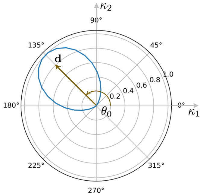
This filter is applied across all positive temporal frequencies . For negative frequencies, the direction needs to be reversed since those waves travel backward in time. Often, a radial component is also added to improve the SNR by eliminating oscillations with unrealistically high wavenumbers. In [SDFIIMR2003MLKE], this radial component is a bandpass Butterworth filter. As we discussed in Section 4, both the directional and radial components are essential for ToF methods.
To see the connection between the PWE method and the directional filter, observe that given a frequency and for each angle , there exists a plane wave that travels in the direction . Because ToF technique relies on directional propagation, we need to manually decompose the shear wave into its directional components specified by angles , process each component separately, and then combine them through compounding. The PWE method on the other hand, searches for dominant directions to capture the shear wave in its entirety (including the reflections and refractions) and to simultaneously compute the wave-speed that best describes the observed data at once. This removes the need for the arbitrary compounding (averaging) step66 6 One could for instance argue for selecting the point-wise maximum of the shear modulus fields instead of averaging. There is no particular advantage to compounding via averaging.and instead selects the shear modulus value considering all data together. To improve the nonlinearity of the PWE optimization problem and at the expense of increasing the dimension of the problem being solved, we explicitly discretized the plane wave directions in (12) to obtain a finite set of plane wave basis functions given by (4). The dominance of each direction in capturing the shear wave is then determined by the magnitude of the corresponding basis coefficient . Note that the plane waves in expansion (3) are fundamental solutions of the scalar wave equation (2) and form a complete set of basis functions meaning that by increasing , we can approximate the solution to the wave equation as closely as we desire [ODHWFEHP2001CK].
Appendix B Nonlinearity of Objective Function
In this appendix, we consider more closely the ability of the PWE method to recover dominant propagation directions and the importance of this ability for reconstructing the desired shear modulus field. We also take a closer look at the shape (nonlinearity) of the objective function in (9) and how the presence of noise and absence of true propagation directions affect it. For simplicity, we use simulated data in a homogeneous medium with shear modulus of = 25 kPa, amounting to a wave-speed of = 5 m/s. We directly fabricate a frequency-domain displacement field using (3) composed of plane waves propagating with uniform angular spacing of at frequency = 600 rad/s. Fig. A2 shows the real component of the field along with a grid of measurements used for elastography.
We choose the coefficients in (3) such that the dominant propagation directions are ordered as .
In Table A.I we study the effect of including the true propagation directions and noise on recovering the dominant propagation directions.
| true directions | noiseless measurements | noisy measurements |
|---|---|---|
| included | ||
| excluded |
To include the true directions, we use whereas to exclude them, we set . Furthermore, we use additive Gaussian noise resulting in SNR dB. In the noiseless case, we set the regularization parameter to whereas in the noisy cases, we use . Observe that when true directions are included, in the absence of noise the true directions are exactly recovered up to their dominancy order. On the other hand, in the presence of noise the last dominant direction is not in the top five selected directions. When the true directions are excluded, the less dominant directions are not closely approximated in the top five propagation directions although plane waves close to these directions might still have high coefficients. The reason for this behavior is that -regularization is known to result in many small coefficients. Using a regularization term in (7) that enhances sparsity helps with better recovering the dominant directions at the expense of higher computational cost but as we show next, exactly recovering these dominant directions is not necessary for accurate shear modulus estimation.
To further elaborate on the last comment, we study the performance of PWE using displacement data corresponding to two frequencies rad/s and rad/s with SNR dB and SNR dB for noisy measurements. Fig. A3 depicts the objective function in (9) for the four different cases of including or excluding true directions and noiseless or noisy data.
Observe that the objective in all cases is extremely non-smooth. Also notice that the individual frequencies can have multiple local minima, some of which might have a smaller objective value than the true wave-speed. Nevertheless, the total objective function summed over the two frequencies often has its global minimum close to the true wave-speed. This shows the importance of using large number of frequencies to ensure that enough information is available for reconstruction. Finally, notice that when the true directions are excluded from reconstruction or data are noisy, the global minimum becomes less prominent. Table A.II reports the estimated constant shear modulus value at each case.
| true directions | noiseless measurements | noisy measurements |
|---|---|---|
| included | ||
| excluded |
Note that although when the true directions are excluded, the dominant directions might not be properly identified as we observed in Table A.I, the PWE method still succeeds in approximating the true shear modulus values.