Building a fault-tolerant quantum computer using concatenated cat codes
Abstract
We present a comprehensive architectural analysis for a proposed fault-tolerant quantum computer based on cat codes concatenated with outer quantum error-correcting codes. For the physical hardware, we propose a system of acoustic resonators coupled to superconducting circuits with a two-dimensional layout. Using estimated physical parameters for the hardware, we perform a detailed error analysis of measurements and gates, including CNOT and Toffoli gates. Having built a realistic noise model, we numerically simulate quantum error correction when the outer code is either a repetition code or a thin rectangular surface code. Our next step toward universal fault-tolerant quantum computation is a protocol for fault-tolerant Toffoli magic state preparation that significantly improves upon the fidelity of physical Toffoli gates at very low qubit cost. To achieve even lower overheads, we devise a new magic-state distillation protocol for Toffoli states. Combining these results together, we obtain realistic full-resource estimates of the physical error rates and overheads needed to run useful fault-tolerant quantum algorithms. We find that with around 1,000 superconducting circuit components, one could construct a fault-tolerant quantum computer that can run circuits which are currently intractable for classical computers. Hardware with 18,000 superconducting circuit components, in turn, could simulate the Hubbard model in a regime beyond the reach of classical computing.
I Introduction
Building a fault-tolerant quantum computer is one of the great scientific and engineering challenges of the 21st century. A successful quantum computing architecture must meet many conflicting demands: it must have an error correction threshold that is achievable by hardware on a large scale, a convenient physical layout, and implement arbitrary quantum algorithms with low resource overhead requirements. All proposed quantum architectures require tradeoffs among these objectives. For example, the most popular proposed architecture, the surface code Bravyi and Kitaev 1998, has a convenient two-dimensional physical layout and relatively high threshold error rates, but the overhead for running useful algorithms remains daunting O’Gorman and Campbell 2017; Motta et al. 2018; Gidney and Ekerå 2019; Campbell et al. 2019; Kivlichan et al. 2020; Chamberland and Campbell 2021, even after years of optimization.
Recent work has shown that qubits with highly biased noise are a promising route to fault tolerance Tuckett et al. 2018; Tuckett et al. 2019; Tuckett et al. 2020; Ataides et al. 2021, at least when gates that preserve the noise bias can be easily implemented in the architecture Aliferis and Preskill 2008; Puri et al. 2020; Guillaud and Mirrahimi 2019; Guillaud and Mirrahimi 2021. One possible route to realizing such qubits is via a two-component cat code Mirrahimi et al. 2014; Puri et al. 2017; Cohen 2017, a bosonic qubit encoded in an oscillator mode Albert et al. 2018; Joshi et al. 2020; Cai et al. 2020, subjected to engineered two-photon dissipation Mirrahimi et al. 2014; Leghtas et al. 2015; Touzard et al. 2018 or an engineered Kerr nonlinearity Goto 2016a; Goto 2016b; Puri et al. 2017; Puri et al. 2019; Grimm et al. 2020. The engineered interaction heavily suppresses population transfer between the two constituent coherent states of the cat qubit, causing an effective noise bias towards phase-flip errors on the cat qubits Mirrahimi et al. 2014; Puri et al. 2017. Experiments suggest that it is possible to engineer highly biased noise with this approach Lescanne et al. 2020. Furthermore, bias-preserving CNOT and Toffoli (TOF) gates can be performed for these cat codes Guillaud and Mirrahimi 2019; Puri et al. 2020.
The performance of dissipative cat qubits is influenced by three key parameters. The average number of excitations in each cat is , which determines the level of noise bias as bit flips are exponentially suppressed with . The rate of phase-flip errors is determined by the competition between two processes: is the single-excitation loss rate (per time) that is the main cause of phase errors; and is the engineered two-excitation dissipation rate (per time) stabilizing the cat-code subspace and suppressing errors. The ratio of these processes is a dimensionless quantity primarily determining the phase-flip error rate. Calculating accurate predictions for is crucial for estimating the performance of cat qubit architectures.
Concatenating the (inner) cat code with another (outer) quantum error-correcting code can reduce qubit requirements by tailoring the outer code to suppress the dominant phase-flip errors. We call these coding schemes concatenated cat codes. While this idea has been explored previously for the case where the outer code is a repetition code Guillaud and Mirrahimi 2019; Guillaud and Mirrahimi 2021, these proposals are completely reliant on increasing to suppress bit-flips errors. As increases, phase errors become more frequent and other physical mechanisms start to become important, so a fully scalable architecture must allow for some bit-flip protection from the outer code. Furthermore, these previous proposals Guillaud and Mirrahimi 2019; Guillaud and Mirrahimi 2021 did not study the rate of bit-flips processes during CNOT gates and did not propose a 2D layout capable of implementing fault-tolerant logic. The lack of such an analysis has left open several urgent questions, such as how a 2D architecture with dissipative cats concatenated with the surface code would perform in practice, and how parameters at the hardware level (such as ) relate to the needs of the larger architecture.
In this paper, we give a full-stack analysis of a fault-tolerant quantum architecture based on dissipative cat codes concatenated with outer quantum error-correcting codes. We propose a blueprint for a possible practical implementation based on hybrid electro-acoustic systems consisting of acoustic resonators coupled to superconducting circuits. These systems are a promising platform for realizing concatenated cat codes due to their small footprint Arrangoiz-Arriola and Safavi-Naeini 2016, potential for ultra-high coherence times MacCabe et al. 2020, and easy integration with superconducting circuits for control and read-out Blais et al. 2021; Arrangoiz-Arriola et al. 2019.
We give a comprehensive error analysis of this approach that provides a detailed picture of the physically achievable hardware parameters (including , and ) and error rates for gates and measurements based on estimated parameters for coupling strengths and phonon loss and dephasing rates. Using the obtained values of the hardware parameters, we then explicitly analyze quantum error correction when the outer code is either a repetition code or a thin rectangular surface code Dennis et al. 2002a; Fowler et al. 2012a. We then show how to build a fault-tolerant quantum computer in our architecture, combining lattice surgery and magic state distillation for Toffoli states. Finally, we provide a resource overhead estimate as a function of physical error rates required to fault-tolerantly run quantum algorithms.
Our analysis can be broadly classified into three categories: 1) a hardware proposal; 2) a physical-layer analysis of gate and measurements errors; and 3) a logical-level analysis of memory and computation failure rates. More specifically, in Section II we describe our hardware proposal for using phononic bandgap resonators and superconducting circuits to store and process quantum information at the physical level. This section provides a range for what hardware parameters are feasible. Then in Section III we give a complete analysis of gate and measurement errors for phononic qubits using realistic noise parameters that we expect from the hardware proposal. In Sections IV, VI, and VII we give a gate-level analysis of universal fault-tolerant quantum computation that looks at logical error rates across a physically relevant parameter regime.
| Capabilities | ||||||||
| REGIME 1 | 3.6 % | repetition code QEC | ||||||
| REGIME 2 | 1.2 % | surface code QEC | ||||||
| REGIME 3 | 0.3 % | useful quantum algorithms |
I.1 Overview of main results
We frame our main results in terms of regimes for the hardware parameters, which we denote REGIME 1, REGIME 2 and REGIME 3, and which we summarize in Table 1. All regimes assume the same number of excitations per cat () but each regime corresponds to a different order of magnitude in the crucial parameter. In REGIME 1, the physical cat-qubit CNOT gate fails with probability , which is well above the threshold for the surface code error correction. However, concatenating cat and repetition codes, REGIME 1 is just below the repetition code phase-flip threshold and so is a suitable regime to demonstrate quantum error correction. In REGIME 2, it is possible to demonstrate small proof-of-principle algorithms with the cat and repetition code. However, while bit-flip errors are rare with , without additional bit-flip protection a quantum computer would decohere before it is able to demonstrate a useful algorithm. In REGIME 2, CNOT gates fail with probability , which is above the usually reported surface code error correction threshold with depolarizing noise. Nevertheless, due to noise bias and other aspects of the noise processes, REGIME 2 would allow a demonstration of fully scalable quantum error correction and computation. However, the surface code overhead remains high in REGIME 2. In REGIME 3, CNOT gates fail with probability and we estimate the resource overhead costs for the task of estimating the ground state energy density of the Hubbard model. For this algorithm, we find fewer qubits are needed than for hardware assuming an unbiased, depolarizing noise model with CNOT gate infidelities of as considered in Ref. Kivlichan et al. 2020. We now summarize in more detail how these conclusions were reached and the technical innovations needed along the way.
In Section II we describe our hardware proposal for using phononic-crystal-defect resonators (PCDRs), of the type reported in Ref. Arrangoiz-Arriola et al. 2019, as the storage elements. These are periodically patterned suspended nanostructures that support localized acoustic resonances in the gigahertz range. They are fabricated from a piezoelectric material such as , which allows us to couple these resonances to superconducting circuits with nearly the same strength as ordinary electromagnetic cavities. Following a recent demonstration Lescanne et al. 2020, we propose implementing the two-phonon dissipation by engineering an interaction through which the storage mode exchanges excitations with an ancillary “buffer” mode in pairs. This buffer is strongly coupled to a bath, so these excitations decay rapidly. We compute for a bath consisting of a multi-pole bandpass filter connected to a semi-infinite transmission line, or waveguide. The filter allows us to control the density of states of the bath, causing it to vanish at all frequencies except those within the filter passband (in this work this is modelled by connecting a dissipative circuit with an appropriate admittance function to the buffer resonator). The filter is useful not only to protect the storage mode from radiative decay, but also plays a crucial role in suppressing correlated phase-flip errors while stabilizing multiple storage modes simultaneously with the same buffer mode.
Given the stringent requirement for , it is ideal to maximize . In our architecture, however, is ultimately limited by crosstalk. Indeed, we find that stronger engineered dissipation can simultaneously lead to increased crosstalk, such that there comes a point where further increasing is no longer beneficial. Specifically, by quantifying crosstalk error rates and calculating their impacts on logical lifetimes, we find that the optimal value is kHz at . This constraint on is discussed further in this section under the Section III summary, and in more detail in Section IV.3. In turn, this imposes the requirement (shown in Table 1) that the intrinsic relaxation time of the storage modes be at least to reach REGIME 3, where it is possible to perform useful quantum algorithms. At present, piezoelectric PCDRs made of can only reach Wollack et al. 2021.
The engineered dissipation needed to stabilize each cat code is provided by coupling each phononic resonator to nonlinear circuit elements. Specifically, we follow the approach of Ref. Lescanne et al. 2020, where the nonlinearity is provided by a circuit element variant of a superconducting quantum interference device (SQUID) called an asymmetrically-threaded SQUID (ATS). While Ref. Lescanne et al. 2020 demonstrated an ATS can be used to stabilize a single mode into a cat code, our hardware layout necessitates that each ATS couple to and stabilize multiple resonators simultaneously. We present a simple scheme for this multiplexed stabilization, and provide a detailed analysis of the crosstalk that arises from coupling multiple modes to the same ATS. Moreover, we show that by employing a bandpass filter and carefully optimizing the phonon-mode frequencies, we are able to largely suppress the dominant sources of crosstalk in our system, though some residual crosstalk remains and we return to discuss this later.
In Section III, we then analyze the errors in our gates and measurements. To do this, we introduce a method that we call the shifted Fock basis method. This method allows us to efficiently perform a perturbative analysis of the dominant error rates of the cat-qubit gates and improve the efficiency of numerical simulation of large cat qubits compared to the usual Fock basis method. The shifted Fock basis method allows us to compute the error rates of various cat-qubit gates using a small Hilbert space dimension that is independent of the average excitation number of the cat qubit.
Using this method, we go on to show that the optimal error rates (per gate) of the cat qubit gates at the optimal gate time scale as . The optimal error rates of the CNOT and TOF gates are in fact independent of the size of the cat qubit, whereas those of and CZ rotations decrease linearly in . We also study the effects of bosonic dephasing and thermal excitations on various cat-qubit gates. Provided these additional effects are small, they do not disturb the noise bias or our main conclusion.
We then develop and analyze schemes for readout in both the and bases, enabling fast and hardware-efficient stabilizer measurements. For -basis readout we propose to use an additional dedicated mode in each unit cell of our architecture. By exchanging the ancilla information with this mode and performing repeated quantum non-demolition (QND) parity measurements in parallel with the gates of the subsequent error correction cycle, we can suppress the infidelity mechanisms associated with the transmon while having minimal impact on the syndrome measurement cycle time. We present a fast and high-fidelity -basis readout using the storage and buffer modes; the resulting error probability decays exponentially as a function of . In the -basis readout scheme, excitation’s are swapped to the buffer mode where they leak to the transmission line and are detected via a homodyne measurement.
With a clear understanding of gate and measurement error rates, we proceed in Section IV to analyze the logical failure rates for a quantum memory based on concatenating the cat code with one of two codes: a repetition code and a thin rectangular surface code. We compute logical failure rates for both the repetition code and the surface code. In the case of the surface code, we compute explicit leading-order failure rates for logical errors as a function of the -distance of the code. Our thresholds are computed using a full circuit-level simulation and a minimum-weight perfect matching (MWPM) decoder. These main simulation results, which inform the conclusions of Table 1, neglected any crosstalk errors. While filters can suppress a wide class of crosstalk errors, there are still residual crosstalk errors that cannot be eliminated by the filters. To investigate this, we perform additional simulations using the detailed information about the residual crosstalk errors from the hardware analysis (Appendix B) and address these errors by adding extra edges in the matching graphs of the surface code decoder. These extra edges are constructed such that they can detect unique syndrome patterns created by the residual crosstalk errors. We find that the performance of the surface code is largely unchanged in the presence of crosstalk, provided that the strength of the engineered coupling between the storage and buffer modes is less than a few MHz (this informs our choice of MHz in Table 1). Were it not for crosstalk, however, the architecture could tolerate stronger engineered couplings and engineered dissipation, which would ease demands on the storage mode coherence. Crosstalk is thus ultimately a limiting factor for our architecture, so we also describe several future research directions that would allow us to further mitigate its effects in future designs.
Using the thin surface code, we consider lattice surgery as a means of performing logical Clifford operations in Section V. By extending our full circuit-level simulation to model timelike errors during lattice surgery, we obtain logical error probabilities for Clifford operations.
To fault-tolerantly simulate universal quantum computation Campbell et al. 2017 with Toffoli gates, we introduce in Section VI a new protocol to fault-tolerantly prepare TOF magic states encoded in the repetition code. Due to the fault-tolerant properties of our protocol, all gates required in our circuits can be implemented at the physical level. Hence we refer to such an approach as a bottom-up approach for preparing TOF magic states. The main insight is that a TOF state can be prepared by measuring a single Clifford observable, which can be achieved using a sequence of physical CNOT and TOF gates. To ensure fault-tolerance, this Clifford measurement has to be repeated a fixed number of times, but due to suppressed bit-flip noise the state does not significantly decohere during this measurement process. Using the full circuit-level noise model of Section III and assuming , we show that TOF magic states can be prepared with total logical failure rates as low as , which is several orders of magnitude lower than what could be achieved using non-fault-tolerant methods to prepare TOF states. Furthermore, the noise on the prepared TOF state is dominated by one specific Pauli error, which is a feature we can further exploit.
In Section VII, we show how TOF magic states probabilistically prepared using our bottom-up approach can be injected in a new magic state distillation scheme. This protocol distills 2 higher-fidelity TOF states from 8 lower-fidelity TOF states with high success probability. For generic noise, the protocol achieves quadratic error reduction. In the relevant case where a single Pauli error dominates, we can achieve cubic error reduction. The protocol is compiled down to architecture-level lattice surgery operations performed at the encoded level using repetition and surface codes. Hence we refer to such an approach as being top-down. Our top-down approach allows us to distill TOF magic states with low enough logical error rates for use in quantum algorithms of practical interest. Further, we note that given the low error rates achieved using our bottom-up approach, only one round of distillation is required in our top-down approach to prepare TOF states with the desired logical error rates.
Finally, in Section VIII we analyze the overhead required for running quantum algorithms in our architecture, based on our estimated gate error rates for REGIME 3. We consider running circuits on 100 qubits with up to 1,000 Toffoli gates, which are comfortably beyond the reach of classical simulability using the best currently known simulation algorithms. For circuits of this size, and for our estimated gate error rates, bit flip errors are sufficiently rare that it suffices to concatenate the cat code with a repetition code. We find that a device with 1,000-2,000 ATS’s could execute the circuit reliably. This number of hardware components is compatible with next generation cryogenic dilution refrigerators, indicating that our proposal holds promise for early implementations of fault-tolerant quantum computation.
For known applications of quantum computing with potential commercial value, substantially larger circuits are needed. Again assuming REGIME 3 parameters, we find that for these larger circuits the cat code should be concatenated with a thin surface code which protects against bit flips as well as phase errors, and the overhead cost is correspondingly higher. As a representative application, we consider the task of estimating the ground state energy density of the Hubbard model. A quantum computer with about 100 logical qubits executing about 1 million Toffoli gates could perform this task in a parameter regime that is very challenging for classical computers running the best currently known classical algorithms. For this purpose we estimate that our architecture could be implemented using 18,000 ATS components and that the quantum algorithm could be executed in 32-89 minutes depending on the physical parameters of the Hubbard model.
Notably, for this problem the magic-state factory uses at most of the total resources and is never a bottleneck on algorithm execution time. This low factory overhead is due to a combination of factors. Firstly, the bottom-up procedure gives initial TOF states with a cost which is not much more than a physical TOF but with orders of magnitude lower error rates. Secondly, at the required TOF error rate it suffices to implement one round of the top-down protocol using a mixture of repetition codes and surface codes, which dramatically reduces the factory footprint. In contrast, the best performing T state factories (in architectures without biased noise) rely completely on surface codes and either require multiple rounds of distillation to achieve the same error suppression Bravyi and Haah 2012; Meier et al. 2013; Campbell and Howard 2018 or only produce 1 T state at a time so that 8 rounds are needed to realize 2 TOF gates Bravyi and Kitaev 2005a.
II Hardware implementation and stabilization schemes
In our proposal, the lowest-level protection from errors occurs directly at the hardware level and is based on the idea of autonomous quantum error correction (QEC) Paz and Zurek 1998, where rather than correcting errors at the “software level”, one instead engineers a system whose unitary evolution and dissipation is sufficient to protect the encoded information from Markovian errors. One can think of this process as the continuous analog of the standard, discrete QEC cycle consisting of syndrome measurements and correcting unitaries. The value of autonomous QEC is that it eliminates the need for active measurements and classical feedback.
Historically, proposals for the implementation of autonomous QEC have been formulated in the language of coherent feedback control Ahn et al. 2002 or reservoir engineering Sarovar and Milburn 2005; Kerckhoff et al. 2010, where the evolution is described via a stochastic master equation or a Lindblad master equation, respectively. Here we specifically adopt a bosonic autonomous QEC technique that more neatly fits into the latter category. It was first introduced by Mirrahimi et al. in 2014 Mirrahimi et al. 2014 and demonstrated for individual qubits in recent experiments Leghtas et al. 2015; Touzard et al. 2018; Lescanne et al. 2020. We summarize the most relevant pieces here for convenience.
II.1 Overview of cat codes and driven-dissipative stabilization
The basic idea is to encode a qubit in a two-dimensional subspace of a harmonic oscillator, spanned by the two quasi-orthogonal coherent states Cochrane et al. 1999; Jeong and Kim 2002. The qubit states can be defined in the basis as the following two-component Schrödinger cat states:
| (1) |
These states are eigenstates of the parity operator with eigenvalues , and . The codewords of this code are
| (2) | ||||
| (3) |
Note that and is a very good approximation for , as will typically be assumed throughout this paper. The notation and is reserved for these cat qubit computational states throughout, and to avoid ambiguity we use and for the vacuum and single phonon (or photon in some alternative architectures) Fock states.

The usual error channels that affect real oscillators, such as energy relaxation and dephasing, will eventually corrupt the information encoded in this manner. To protect against these common errors, one can engineer an artificial coupling to a bath such that the oscillator only emits and absorbs excitations to and from this bath in pairs. Such dynamics can be modeled by a Lindblad master equation of the form
| (4) |
where , is the usual single-phonon (or photon) dissipation rate, is the pure dephasing rate, and is a two-phonon (or two-photon) dissipation rate. In the case where , any linear combination of the codewords is a steady state of Eq. 4. This is straightforward to see, as any state for which is stationary under this master equation, and this includes both the even- and odd-parity cats. Furthermore, outside this subspace, there are no further steady states of the Lindblad master equation. Therefore, any initial state will eventually evolve to a mixture of states within this subspace. We refer to the rate at which this decay happens as the confinement rate, ; using the displaced Fock basis (see Appendix C) one can show that . For finite , this description of the dynamics no longer holds true exactly. In particular, the stationary solutions of Eq. 4 are no longer pure states. However, if , where is the effective error rate, then the codewords are still metastable states. The threshold depends on the error channel in question: for phonon (or photon) loss, and for dephasing Lieu et al. 2020.
The key feature of this code is that, above the threshold , the bit-flip rate (or rate of -type errors) decays exponentially with the “code distance” as
| (5) |
where for phonon (or photon) loss Guillaud and Mirrahimi 2021 and for dephasing Mirrahimi et al. 2014. On the other hand, the phase-flip rate (or rate of -type errors) increases linearly as
| (6) |
For sufficiently small values of the dimensionless loss parameter , and sufficiently large , this translates to a large noise bias, i.e. a large discrepancy between the and error rates. As alluded to earlier, this bias is a key feature of our proposal and will be exploited when designing the outer error-correcting codes.
The driven-dissipative dynamics of Eq. 4 can be physically realized by using a cleverly designed nonlinear element to couple the storage mode to an engineered environment, or reservoir. Following Refs. Leghtas et al. 2015; Lescanne et al. 2020, the idea is to generate a nonlinear interaction of the form between the storage mode and an ancillary mode , which here we refer to as the “buffer mode” in keeping with existing terminology. The buffer mode is in turn strongly coupled to a bath — it is designed to have a large energy relaxation rate so that it rapidly and irreversibly emits the photons it contains into the environment. If , the mode is in the vacuum state most of the time, and its excited states can be adiabatically eliminated from the Hamiltonian Reiter and Sørensen 2012; Leghtas et al. 2015. In this picture, there exists an effective Markovian description of the mode dynamics where the mode is considered as part of the environment and where the emission of excitations via can be accurately modeled as a dissipative process acting on the mode alone. To stimulate the absorption process a linear drive on the buffer mode is added to supply the required energy. With this drive tuned on resonance with the buffer (), the evolution of the combined system is described by
| (7) |
where . After adiabatically eliminating the mode, this master equation becomes Eq. 4, with .
II.2 Physical implementation of buffer and storage resonators
To realize the dynamics described by Eq. 7 in practice, previous demonstrations of two-phonon dissipation have relied on Josephson junctions Leghtas et al. 2015; Touzard et al. 2018 or an “asymmetrically-threaded SQUID” (ATS) Lescanne et al. 2020 as the source of nonlinearity. Other variations of the nonlinear elements exist, for instance the “SNAIL” Frattini et al. 2017; Grimm et al. 2020, but in this proposal we adopt the ATS due to the advantages it has over other nonlinear elements. These advantages are outlined in Ref. Lescanne et al. 2020.
The potential energy of an ATS has the form , where is the superconducting phase difference across the ATS and are vacuum fluctuation amplitudes that quantify the contribution of the and modes to the phase . It is important to emphasize that here are the normal modes of the combined storage and buffer resonators. Because these resonators are far-detuned, there is little mixing between them, so is “storage-like” and is “buffer-like”.
Terms of cubic and higher orders in the power-series expansion of generate nonlinear couplings between the modes, provided that the required energy is injected with pumps tuned to the appropriate frequencies. The desired interaction can be resonantly activated by modulating the magnetic flux that threads the ATS at frequency . This modulation, which from now on we refer to as the “pump”, provides the missing energy in the conversion process — two storage phonons get converted to a buffer photon and pump photon. To stimulate the reverse process — the conversion of a buffer and a pump photon to two storage phonons — a linear drive at frequency is applied to the buffer. From now on we refer to this simply as the “drive”. For further details on the implementation and the calculation of , see Appendix A and Ref. Lescanne et al. 2020.
For the storage oscillator, the three cited experiments have used either superconducting 3D microwave cavities Leghtas et al. 2015; Touzard et al. 2018 or on-chip coplanar-waveguide (CPW) resonators Lescanne et al. 2020, and recent theoretical proposals have focused on similar implementations Guillaud and Mirrahimi 2019; Guillaud and Mirrahimi 2021. Here we study the possibility of using nanomechanical resonators instead, and tailor our calculations specifically to the case of one-dimensional phononic-crystal-defect resonators (PCDRs) made of lithium niobate, a crystalline piezoelectric material. These devices support resonances at gigahertz frequencies, with modes that are localized inside a volume of a suspended nanostructure. They have been coupled to transmon qubits in recent experiments Arrangoiz-Arriola et al. 2019; Mirhosseini et al. 2020 and may offer a number of advantages over electromagnetic resonators.
First, a PCDR is a micron-scale nanostructured device, with an on-chip footprint (area) that is at least three orders of magnitude smaller than that of planar superconducting resonators, including lumped-element structures. This is not a significant advantage today, with the largest quantum computers only having a few dozen physical qubits, but it may become important in the future.
A second consideration is that, unlike electromagnetic resonators, appropriately designed acoustic devices do not experience direct crosstalk (unwanted couplings) because acoustic waves do not propagate through vacuum. They can still couple through the circuitry that mediates interactions between them, but this can be mitigated with approaches such as filtering and a carefully chosen connectivity, both of which are important features of our proposal.
The third and most important consideration is that there is recent experimental evidence that phononic-crystal-based devices can have very long coherence times as a result of the high degree of confinement of their modes and the quality of their materials. For example, devices fabricated from silicon and operating at a frequency of have been shown to have energy relaxation and pure dephasing times of and , respectively MacCabe et al. 2020. These silicon devices cannot be easily coupled to superconducting circuits, but they offer insight into the decoherence mechanisms affecting nanomechanical resonators and suggest a roadmap for achieving similar levels of coherence with piezoelectric devices. For example, similar studies with lithium niobate PCDRs are already under way Wollack et al. 2021, and although their coherence times are currently limited to , it is possible their performance could approach that of the silicon devices after sufficient advances in materials and surface science.
We remark that although we have tailored our calculations to the case of PCDRs, the results of this proposal are still applicable to a setting where the storage modes are electromagnetic.
II.3 Wiring and layout
We now describe a way to combine all of these building blocks to build a two-dimensional grid of cat qubits that form the basis for an outer code, such as the repetition code or the surface code. First, following Ref. Lescanne et al. 2020 we form a buffer resonator with frequency by shunting an ATS with a capacitor. This buffer mode is then coupled to the input of a bandpass filter that passes frequencies within a bandwidth centered at and attenuates frequencies outside this range. The output of the filter is connected to an open waveguide (which can be accurately modeled as a resistive termination). This filter configuration stands in contrast to the implementation in Ref. Lescanne et al. 2020, where a bandstop filter (that instead attenuates frequencies within some band and passes all others) was used to protect the storage mode from radiatively decaying into the waveguide. In our proposal, the bandpass filter also serves this role, but it also plays a more fundamental role as a means of suppressing crosstalk mechanisms that arise as a result of our frequency-multiplexed scheme to stabilize (and perform gates between) multiple modes with a single ATS. From this point on, we refer to the combination of the buffer, filter, and waveguide as the “reservoir”.
We arrange reservoirs in a two-dimensional grid, as shown in Fig. 2, and connect neighboring reservoirs with a PCDR using each of the two terminals of the resonator. The reservoirs provide the connectivity between resonators and are located above, below, to the left, and to the right of each resonator. These four resonators serve as data and ancilla qubits in either the repetition or the surface code. In addition, one more resonator coupled to each reservoir serves the purpose of an ancillary readout mode which is used to measure the cat qubits in the basis with the aid of a ordinary transmon. Alternatively, it is possible to omit this resonator altogether and perform the readout directly via the buffer — see Appendix H for further details.
There are two important considerations that motivate this architecture. The first is that present PCDR designs only have two available terminals, so each of them can be connected to at most two different reservoir circuits. This is simply a design choice — it may be possible to add more terminals without a significant degradation of performance, and this would enable other variations of the 2D layout. The second consideration comes from our analysis of correlated errors in the frequency-multiplexed stabilization scheme, which we overview below and provide details of in Appendix B. Our results show that the correlated error rates increase rapidly with the number of modes connected to an ATS, and the error rates that come with choosing five modes per ATS are the largest that can be tolerated by the outer error-correcting codes.
II.4 Estimation of dissipation rates and
The dissipation rates and are crucial parameters: they set the error rates of the gates, as well as the error rates during idling, state preparation, and measurement. Two-phonon loss is an engineered process, so the two-phonon loss rate is a parameter that we can calculate. On the other hand, the single-phonon loss rate is largely determined by intrinsic properties of the hardware. To construct the error model we use in this proposal, then, the starting points are to 1) calculate a prediction for the maximum achievable value of , and 2) infer the values of that are required to reach various regimes of interest. We will consider three distinct regimes in this proposal, characterized by the magnitude of the “dimensionless loss” parameter : (REGIME 1), (REGIME 2), and (REGIME 3). This parameter is particularly important because the -type error rates scale as for both the CNOT and Toffoli gates (see Section III and Table 2 for further details). These regimes are summarized in Table 1.
A summary of our calculation is presented next, with further details contained in Appendix A. As described previously, the way the two-phonon loss is engineered is by inducing a nonlinear coupling between the storage mode and a buffer mode , which decays into the environment at rate . A key requirement is that , so that the excited states of the buffer can be adiabatically eliminated to yield an effective description where the storage directly experiences two-phonon loss. In this adiabatic regime, . We may write the adiabaticity constraint as for some . We have observed numerically that is sufficient to stabilize high-fidelity cat states. Putting this together, we find that the maximum achievable two-phonon dissipation rate scales linearly with the buffer decay rate and inversely with the mean phonon number (the “distance” of the cat code):
| (8) |
We note that the maximum achievable is upper bounded by the filter bandwidth, (see Appendix A for details). In this work, we fix MHz, which is sufficient to satisfy for the values of we consider.
We now move on to estimating the required values of the single-phonon loss rate . Before doing so, we first recall that and are the normal — or hybridized — modes of the system, and therefore is given by
| (9) |
Here is the linear coupling rate between the bare storage and buffer resonators, is their detuning, and is the intrinsic decay rate of the bare buffer resonator. The first contribution is the intrinsic loss rate of the bare storage mode, an empirical quantity that depends, for example, on the quality of the resonator materials. The second contribution is due to direct radiative decay into the buffer bath, which we make negligibly small by ensuring the storage frequency lies far outside of the filter passband, or in other words by ensuring the bath has a vanishing density of states at . The third contribution is due to the intrinsic loss of the bare buffer resonator, which the storage inherits due to their hybridization and which the filter cannot protect against. Usually , so this last contribution is important when .

Summing up, when the buffer bath has a vanishing density of states at . A key result of our analysis is that can be strongly suppressed by using a buffer resonator with a large characteristic impedance . This can be accomplished by increasing until is suppressed to a value comparable to or smaller than . This comes at the cost of reducing the nonlinear interaction rate , which also scales with the detuning as . But one can offset this penalty by increasing , because as we show in Appendix A. We show that under certain assumptions of and , once we can access a regime where and therefore
| (10) |
This is a useful result, as it addresses the problems that arise when coupling a highly coherent, linear storage element to a much lossier superconducting circuit. In Fig. 3, we plot this simple expression for as a function of and . We assume , which is large enough to result in good performance of the outer codes.
In later sections, we analyze the performance of our architecture and find that there is an upper limit on , beyond which crosstalk begins to inhibit the performance of the architecture. Specifically, in Section IV.3, we show that the nonlinear coupling strength must satisfy MHz, lest crosstalk degrade the logical lifetimes. As a result, we have the restriction that MHz. At this maximal value, the values needed to reach the three different regimes we study in this paper are indicated in Fig. 3 (see also Table 1). Because crosstalk is thus a limiting factor for our architecture, we remark that there are several ways crosstalk could be mitigated in future designs. For example, in Appendix H, we describe an alternative version of our architecture with 4 modes per unit cell as opposed to 5; this modification reduces crosstalk, thereby enabling larger and easing the requirements. Future approaches could reduce the number of modes per unit cell even further by increasing the number of terminals of each PCDR.
It is important to note that the value that we derive in this analysis, while theoretically possible, would require a larger values of (about 5 times larger) than those previously reported Lescanne et al. 2020. Because (see Section II.1), this would require a larger drive amplitude on the buffer mode in order to maintain a fixed , which may cause unforeseen problems such as instabilities Lescanne et al. 2019 or the excitation of spurious transitions Sank et al. 2016; Zhang et al. 2019. Furthermore, the large buffer impedance required increases the size of the vacuum fluctuations of the superconducting phase , making the system more prone to instabilities. A detailed analysis of the power-handling capacity of our system is beyond the scope of this work. This is an area of active research, with promising advances such as the use of inductive shunts to suppress instabilities Verney et al. 2019.
II.5 Multiplexed stabilization
In our architecture, each reservoir is responsible for stabilizing multiple storage modes simultaneously, in contrast to prior proposals Mirrahimi et al. 2014; Guillaud and Mirrahimi 2019. This multiplexed stabilization is both beneficial and necessary in the context of our architecture. Stabilizing multiple storage modes with a single reservoir is clearly beneficial from the perspective of hardware efficiency, as the required number of ATSs and control lines is reduced. Moreover, the use of PCDRs (as opposed to, e.g., electromagnetic resonators) actually necessitates multiplexed stabilization. Current PCDR designs have only two terminals, meaning that a PCDR can couple to at most two different reservoir circuits, yet each reservoir must couple to at least four storage modes in order to achieve the required 2D-grid connectivity. Each reservoir must necessarily stabilize multiple storage modes as a result.
Conveniently, we find that multiplexed stabilization can be implemented via a simple extension of the single-mode stabilization scheme demonstrated in Ref. Lescanne et al. 2020. The main idea is to use frequency-division multiplexing to stabilize different modes independently. Here, multiplexing refers to the fact that different regions of the filter passband are allocated to the stabilization of different modes. When the bandwidth allocated to each stabilization process is sufficiently large, multiple modes can be stabilized simultaneously and independently, as we now show.
To stabilize the -th mode coupled to a given reservoir, we apply a pump frequency , and drive the buffer mode at frequency , where denotes a detuning. To stabilize multiple modes simultaneously, we apply multiple such pumps and drives. Analogously to the single-mode stabilization case, the nonlinear mixing of the ATS then gives rise to an interaction Hamiltonian of the form
| (11) |
see Appendix B for derivation. Note that the sum does not run over all modes coupled to the ATS, but rather only over the modes stabilized by that ATS. In our architecture, though five modes couple to each ATS, only two must be stabilized simultaneously, so the sum contains only two terms. By adiabatically eliminating the lossy buffer mode, and assuming the detunings are chosen such that for all , one obtains an effective master equation describing the evolution of the storage modes,
| (12) |
see Appendix B for derivation. Here, if the corresponding detuning falls inside the filter passband (), and otherwise, see Appendix A. The dynamics (12) stabilize cat states in different modes independently and simultaneously. Thus, by simply applying additional pumps and drives with appropriately chosen detunings, multiple modes can be simultaneously stabilized by a single ATS.
The efficacy of this multiplexed stabilization scheme can be understood intuitively by considering the frequencies of photons that leak from the buffer mode to the filtered bath. In the case of , a pump applied at frequency facilitates the conversion of two phonons of frequency to a single photon of frequency (note that acoustic phonons are converted into buffer photons via piezoelectricity in our proposal). As a result, photons that leak from the buffer to the bath have frequency . If instead the pump is detuned by an amount , it follows from energy conservation that the corresponding emitted buffer mode photons have frequency . When the differences in these emitted photon frequencies, , are chosen to be much larger than the emitted photon linewidths, (see Appendix C), emitted photons associated with different storage modes are spectrally resolvable by the environment. Therefore, when the stabilization of mode causes a buffer mode photon to leak to the environment, there is no back-action on modes . These ideas are illustrated pictorially in Figure 4(a).
II.6 Crosstalk
Our multiplexed stabilization scheme can induce undesired crosstalk among the cat qubits, and this crosstalk must be quantified in order to provide realistic performance estimates for our architecture. We now enumerate the different sources of crosstalk and show that the dominant sources can be largely suppressed through a combination of filtering and phonon-mode frequency optimization. Later on, in Section IV, we incorporate the residual crosstalk errors into calculations of the logical error rates for our architecture, finding that these small correlated errors can nevertheless be a limiting factor for overall performance.
In acting as a nonlinear mixing element, the ATS not only mediates the desired interactions, but it also mediates spurious interactions between different storage modes. While most spurious interactions are far detuned and can be safely neglected in the rotating-wave approximation, there are others which cannot be neglected. Most concerning among these are interactions of the form
| (13) |
for , where . This interaction converts two phonons from different modes, and , into a single buffer mode photon, facilitated by the pump that stabilizes mode . These interactions cannot be neglected in general because they have the same coupling strength as the desired interactions (11), and they can potentially be resonant or near-resonant, depending on the frequencies of the storage modes involved.
There are three different mechanisms through which the interactions (13) can induce crosstalk among the cat qubits. These mechanisms are described in detail in Appendix B, and we summarize them here. First, analogously to how the desired interactions (11) lead to two-phonon losses, the undesired interactions (13) lead to correlated, single-phonon losses
| (14) |
where the rate will be discussed shortly, and is the logical Pauli- operator for the cat qubit in mode . The arrow denotes projection onto the code space, illustrating that these correlated losses manifest as stochastic, correlated phase errors in the cat qubits.
Second, the interplay between different interactions of the form (13) gives rise to new effective dynamics James and Jerke 2007a; Gamel and James 2010; Reiter and Sørensen 2012 generated by Hamiltonians of the form
| (15) | ||||
| (16) |
where the coupling rate is defined in Appendix B. The projection onto the code space in the second line reveals that can induce undesired, coherent evolution within the code space.
Third, can also evolve the system out of the code space, changing the phonon-number parity of one or more modes in the process. Though the engineered dissipation subsequently returns the system to the code space, it does not correct changes to the phonon-number parity. The net result is that also induces stochastic, correlated phase errors in the cat qubits,
| (17) |
where the rate will be discussed shortly.
Remarkably, all of the stochastic crosstalk errors, (14) and (17), can be suppressed to negligible levels through a combination of filtering and phonon-mode frequency optimization. In Appendix B, we show that both and , provided
| (18) | ||||
| (19) |
respectively. This suppression can be understood as follows. The decoherence associated with and results from the emission of buffer mode photons at frequencies and , respectively. When the frequencies of these emitted photons lie outside the filter passband, their emission (and the associated decoherence) is suppressed. Crucially, we can arrange for all such errors to be suppressed simultaneously by carefully choosing the frequencies of the storage modes, as shown in Figure 4(b,c). We note that the configuration of mode frequencies in Figure 4(c) was found via a numerical optimization procedure described in Appendix B and is robust to realistic frequency fluctuations.
The coherent crosstalk errors (16) can also be suppressed through phonon-mode frequency optimization, though the suppression is not sufficient to render them negligible. To suppress these errors, the phonon-mode frequencies have been chosen to maximize the detunings , such that is rapidly rotating and its damaging effects are mitigated to a large extent (see Appendix B for details). Even so, the residual crosstalk errors are not negligible and they must be accounted for when estimating the overall performance of the architecture. To this end, in Appendix B we precisely quantify the magnitude of these residual crosstalk errors, and the impact of these errors on logical failure rates is calculated in Section IV. As described in that section, we must have MHz, lest these coherent errors degrade logical lifetimes. At the hardware level, this restriction limits the achievable (see Section II.4), meaning that longer storage mode coherence times are required to reach a given because of these coherent crosstalk errors.
Crosstalk also imposes another limitation on our architecture: though increasing the number of modes per unit cell would improve hardware efficiency and connectivity, crosstalk forces us to minimize the number of modes per unit cell. Indeed, as more modes are added to a unit cell, frequencies become increasingly crowded Naik et al. 2017; Pechal et al. 2018; Hann et al. 2019, and magnitude of crosstalk errors increases. Accordingly, we have chosen four modes (plus one additional mode for readout) per unit cell because this is the minimum number consistent with our 2D square grid layout. In Appendix H, we describe an alternative architecture that only uses four modes per unit cell, but requires a different approach to measurements that may be more challenging to implement.
Broadly speaking, these limitations illustrate the importance of accounting for crosstalk when designing and analyzing fault-tolerant quantum computing architectures. More specifically, these limitations reveal that finding further ways to mitigate crosstalk is an important direction for future research on dissipative cat qubits. In future designs, resonators with additional terminals, or tunable couplers Mundada et al. 2019; Chen et al. 2014, could be employed to further mitigate the effects of crosstalk, for example. Additionally, in Appendix H, we describe an alternate version of our architecture that employs a different -basis readout scheme in order to reduce the number of modes per unit cell and hence reduce crosstalk.
III Gates and Measurements
In this section, we discuss the gates and measurements of the cat qubits. We first discuss the implementation of the gate via a rotating two-phonon dissipation; this will be helpful for understanding the CNOT and Toffoli gates. We then review the fundamentals of the bias-preserving CNOT and Toffoli gates acting on cat qubits Guillaud and Mirrahimi 2019 and present several new analytical and numerical results. In particular, we explicitly characterize the extra geometric phase ( or CZ rotations) which must be taken into account in the implementation of the CNOT and Toffoli gates if the average excitation number is not an even integer. Moreover, we introduce the shifted Fock basis method and demonstrate that it is useful for the perturbative analysis of the error rates of various cat-qubit gates. We then illustrate that the shifted Fock basis method also allows more efficient numerical simulation of large cat qubits (up to ) than the usual Fock basis method. The numerical results on gate error rates are summarized in Table 2 and detailed descriptions of the methods are given in Appendices C, D and E. These results are fed into the simulations of the concatenated cat codes in Sections IV and VI.
We also describe schemes for - and -basis readout. Our scheme for -basis readout has only a small impact on the length of an error correction cycle, thanks to the use of an additional readout mode that is interrogated by a transmon in parallel with the next error correction cycle. We also present a fast -basis readout scheme which uses a coupling between the storage mode and buffer mediated by the ATS. This achieves measurement error rates which improve exponentially as increases. Having hardware native - and -basis readout schemes allows for higher fidelity surface code stabilizer measurements as explained in Section IV.2. A more detailed analysis of the readout schemes can be found in Appendix G. Additionally, in Appendix H we present an alternative -basis readout scheme where the readout is performed directly using the ATS, obviating the need for the extra readout mode and transmon.
III.1 X Gate
The gate interchanges the cat-code computational basis states and . For large values of these cat-code states are approximately equal to the coherent states and , so the gate acts by rotating the coherent states by in the phase space representation. The value of for the stabilized cat state is given by (c.f. Section II.1), so that the phase of is determined by the phase of the drive. Therefore, modulating the phase of the drive on the storage cavity such that the stabilized value of rotates by over a time realizes an gate. The code state evolves according to
| (20) |
This gives an adiabatic implementation of the gate. Furthermore, we can apply a compensating Hamiltonian given by
| (21) |
so that the code state rotates along with the fixed point of the dissipator. With this compensating Hamiltonian, the gate need not be adiabatic and will succeed for any . When the gate is corrupted by phonon loss, gain, or by dephasing, the logical error rates during the gate are identical to the noise during idle. This is because in the rotating frame of the compensating Hamiltonian , the noise and the dissipator are identical to the case of idle. The error rates for idle are summarized in Table 2.
III.2 CNOT
We can realize the bias-preserving CNOT gate from Guillaud and Mirrahimi 2019 using an ATS coupled to a pair of acoustic modes. The CNOT gate rotates the cat-code states of the target mode just as for the gate, except that now the rotation is conditioned on the state of the control mode. Cavity mode 1 will be the control and cavity mode 2 the target. A time dependent dissipator that realizes this rotation is given by the Lindblad jump operator
| (22) |
When cavity mode 1 is in the cat-code state, which is approximately equal to the coherent state, the corresponding dissipator reduces approximately to the rotating dissipator for the gate on the second cavity mode. On the other hand when cavity mode 1 is in the cat state, the operator reduces to the usual time-independent Lindblad operator. The control cavity mode is always stabilized by the usual time-independent Lindblad operator:
| (23) |
When a cat-code state evolves according to
| (24) |
the encoded state undergoes a CNOT gate (up to an extra rotation on the control qubit; see below), assuming the gate time is long compared to the stabilization rate . This gate preserves the bias in the noise because the two cat-code states remain distantly separated during the conditional rotation.
Just as for the gate the CNOT gate can be performed much faster with the help of a compensating Hamiltonian. In this case, an ideal compensating Hamiltonian would be . This Hamiltonian rotates the state of mode 2 conditioned on the state of mode 1, so that the two-mode system remains in the subspace stabilized by the static dissipator and the rotating dissipator . However, such a compensating Hamiltonian is highly nonlinear and would be hard to implement in practice. Hence, as in Ref. Guillaud and Mirrahimi 2019, we consider an approximate version of the above Hamiltonian which only requires at most third-order nonlinearities: In this case the compensating Hamiltonian has the form:
| (25) |
This Hamiltonian rotates the state of mode 2 conditioned on the state of mode 1, so that the two-mode system remains in the subspace stabilized by the dissipator and the rotating dissipator .
The dissipators and combined with the compromised version of the compensating Hamiltonian in Eq. 25 implement a gate
| (26) |
in the limit, which differs from the desired CNOT gate by an extra rotation on the control qubit (see Appendix D for more details). Here, is defined as and is a computational basis state, the eigenstate of the Pauli operator. The extra rotation is trivial if the average excitation number is an even integer. We also remark that the extra rotation is not present if an ideal compensating Hamiltonian is used.
Since the compensating Hamiltonian in Eq. 25 is only an approximation of an ideal compensating Hamiltonian, e.g., (i.e., ), it introduces a residual non-adiabatic error that scales like , where is the gate time. Phonon loss, gain, and dephasing noise during the CNOT gate give rise to a error rate on both cavities that is proportional to . The balance between the non-adiabatic errors and the noise gives rise to an optimal gate time that maximizes the fidelity.
In Ref. Guillaud and Mirrahimi 2019, it was noticed that the residual non-adiabatic error scales as and found that the constant coefficient is given by via a numerical fit. In Appendix D, we provide a first-principle perturbative analysis of the error rates of the CNOT gate by using the shifted Fock basis as a main tool. The key idea of the shifted Fock basis is to use the displaced Fock states as the (unorthonormalized) basis states, where is the mode occupation number. In particular, for the perturbative analysis of the error rates, it suffices to consider only the ground state manifold consisting of the coherent states and the first excited state manifold consisting of the displaced single-phonon Fock states . See Appendix C for a detailed description of the shifted Fock basis, including orthonormalization and matrix elements of the annihilation operator in the shifted Fock basis. By taking the ground and the first excited state manifolds in the shifted Fock basis and using perturbation theory, we find that the error rates (per gate) of the implemented gate are given by
| (27) |
Here, is the single-phonon loss rate (per time) and we assumed no dephasing and gain for the moment. We use for error rates predicted by the perturbation theory and for numerical results. Note that the coefficient in the non-adiabatic error term is close to the coefficient which was found earlier via a numerical fit Guillaud and Mirrahimi 2019. Hence, the optimal gate time that minimizes the total gate infidelity is given by
| (28) |
and at the optimal gate time, the error rates are given by
| (29) |
These agree well with the numerical results (see Table 2)
| (30) |
within a relative error of (see Appendix D for the reasons for the discrepancy). Note that the perturbation theory predicts that the optimal error rates of the gate (or the CNOT gate for even ) are independent of the size of the cat code .
We simulated the CNOT gate using the effective dissipators and Hamiltonian acting on two cavities. Our method was to use the shifted Fock basis as described in Appendix C to find the optimal gate time and perform tomography at the optimal gate. This allowed us to compute all of the two-qubit Pauli error rates. The shifted Fock basis approach allowed us to compute the error rates with a small Hilbert space dimension that does not depend on . In the standard Fock basis the required Hilbert space dimension increases rapidly with . In contrast to the error rates, to accurately resolve the full set of Pauli error rates a large dimension that increases with is required even for the shifted Fock basis. However, even for the full set of Pauli error rates, our simulations are several times faster when we use the shifted Fock basis rather than the standard Fock space, because good accuracy can be attained using a smaller Hilbert space dimension.
Our code was written in Python using the QuTIP package to solve the master equation including the disspators and Hamiltonian terms. We ran the simulations using AWS EC2 C5.18xlarge instances with 72 virtual CPUs, and the total time required for the CNOT simulations was about 150 hours.
III.3 Toffoli
The bias-preserving Toffoli or CCX gate is directly analogous to the CNOT gate. The two control modes are stabilized by the usual jump operator and , while the third mode is stabilized by a jump operator that couples the three modes and rotates the third conditioned on the state of the two controls,
| (31) |
When both modes 1 and 2 are in the cat-code state, this jump operator reduces to approximately , which is the rotating jump operator that realizes the gate on the third mode. When one of the control modes is in the cat-code state, the jump operator is approximately equal to the usual jump operator that stabilizes the cat-code states. In this way the jump operators , , and implement the Toffoli gate (up to a controlled- rotation on the two control qubits). Also like the CNOT gate we can apply a Hamiltonian to drive the desired evolution and perform the gate much faster while canceling part of the non-adiabatic errors. For the Toffoli gate this Hamiltonian is given by
| (32) |
This Hamiltonian is the natural extension of Eq. 25. It does not cancel all non-adiabatic noise, and like the CNOT in the presence of noise, the trade-off between non-adiabatic errors and noise from loss or dephasing gives rise to an optimal gate time for each value of and the noise parameters.
Similarly as in the case of the CNOT gate, we emphasize that the dissipators , , and combined with the compensating Hamiltonian in Eq. 32 realize a gate
| (33) |
which differs from the desired Toffoli gate by a CZ rotation on the two control qubits (see Appendix D for more details). Here, is defined as and is the simultaneous eigenstate of the Pauli operators and . The extra CZ rotation is not present if an ideal compensating Hamiltonian is used. Note that the extra CZ rotation is trivial if is an even integer.
We simulated the Toffoli gate subject to phonon loss, gain, and dephasing at different rates by solving the master equation given by the Hamiltonian , the dissipator on each mode, and the Lindblad operators for the noise. These simulations were carried out using AWS EC2 c5.18xlarge instances and took about 170 hours running on instances with 72 virtual CPUs. Because we simulated three modes for the Toffoli gate, we were able to resolve only the dominant -type error rates and not the other Pauli error rates that are exponentially small in . These simulations used the shifted Fock basis approach. With this method we are able to use a Hilbert space dimension of for each of the three modes and simulate all of the Pauli error rates with high precision. The numerical results for the optimal gate time and the 7 -type Pauli error rates under a pure loss noise model are summarized in Table 2. The results including gain and dephasing can be found in Table 8. Our simulations match our perturbation theory calculations for the error rates.
Similarly as in the case of the CNOT gate, we can use the ground and the first excited state manifolds in the shifted Fock basis and perform a perturbative analysis. Our perturbation theory yields the following error rates of the gate, or the Toffoli gate when is an even integer (see Appendix D):
| (34) |
Note that, the optimal gate time that minimizes the total gate infidelity is given by which is identical to the optimal gate time of the gate (or the CNOT gate for even ) predicted by the perturbation theory. At the optimal gate time, the error rates (per gate) are given by
| (35) |
which agree well with the numerical results (see Table 2)
| (36) |
up to a relative error of . Thus, as in the case of the CNOT gate, the perturbation theory predicts that the optimal error rates of the gate (or the Toffoli gate for even ) are independent of the size of the cat code.
| REGIME 1 | REGIME 2 | REGIME 3 | Formula | |
| () | () | () | ||
| CNOT | ||||
| Optimal Gate Time | ||||
| Toffoli at CNOT optimal Time | ||||
| Prep | ||||
| Time | ||||
| Error Probability | ||||
| Prep | ||||
| Time | ||||
| Error Probability | ||||
| Idle | ||||
| Error Probability | ||||
| Error Probability | ||||
| Error Probability |
| REGIME 1 | REGIME 2 | REGIME 3 | |
| Measurement | |||
| Idling Time | |||
| Infidelity Repetition Code | |||
| Infidelity Surface Code | |||
| Measurement | |||
| Infidelity |
III.4 measurement
-basis readout entails determining the parity of a bosonic mode. Specifically this is readout in the basis of even and odd cat states, i.e., . Here we describe our approach to -basis readout. In our scheme, we use an additional phononic readout mode in every unit cell that we do not stabilize with two phonon dissipation. This readout mode is interrogated by a transmon qubit in parallel with the gates of the next error correction cycle. This allows us to achieve high measurement fidelity and minimal idling time for the data qubits. The additional readout mode (coloured green) and transmon are pictured in Fig. 2.
Here we outline the steps for the readout of an ancilla qubit in the basis. First we “deflate” the ancilla mode () which maps the even parity cat state to the Fock state and the odd cat state to the Fock state Grimm et al. 2020. This can be achieved by abruptly changing the engineered dissipation from to . Pairs of phonons will be dissipated mapping the system to the and manifold while preserving parity. The purpose of the deflation is to reduce susceptibility to single-phonon loss events which change the parity of the cat qubit. After this deflation we turn off the two-phonon dissipation. Subsequent to the deflation the ancilla mode and readout mode () evolve under the Hamiltonian which transfers the excitation Gao et al. 2018; Zhang et al. 2019; Gao et al. 2019 between the ancilla mode and readout mode in a time .
With the excitation in the readout mode, we perform repeated QND (quantum non-demolition) measurements of the readout mode Sun et al. 2014; Hann et al. 2018; Elder et al. 2020 and take a majority vote to get our final measurement outcome. The individual measurements are standard QND bosonic parity measurements which are performed using a dispersive coupling between the readout mode and a transmon qubit () described by . Evolution under the Hamiltonian for a time yields the controlled parity gate . Combined with transmon state preparation and measurement this interaction can be used to realize parity measurements of the readout mode Sun et al. 2014.
While this repeated parity measurement is taking place, the CNOT gates of the next error correction cycle can occur in parallel. This enables us to reach high readout fidelity without affecting the length of an error correction cycle. For our repetition code and surface code simulations we use up to 3 or 5 parity measurements respectively during the error correction gates of the next cycle.
We simulated this measurement scheme to get a rough sense of the expected measurement fidelities. The misassignment probabilities and measurement idling times can be found in Table 3 for the three regimes considered in the paper.
III.5 measurement
In -basis measurement the goal is to distinguish and , which are approximately the coherent states and . We achieve this readout by engineering a coupling between the storage model and the buffer mode described by the “beamsplitter” Hamiltonian . The physical realization of this Hamiltonian is explained in Appendix G.
If the state of the storage mode is , this coupling drives the buffer mode to a coherent state whose phase is aligned with the initial phase of the storage mode. Hence a homodyne measurement of the buffer mode distinguishes the states of the storage mode, as desired.
In Appendix G we find that the signal to noise ratio (SNR) for this readout scheme at time is
| (37) |
in good agreement with numerics. Here is the single-phonon loss rate of the buffer mode, and . The measurement SNR scales as which means there is an exponential improvement of the measurement fidelity with . This measurement process is not quantum non-demolition (QND) and at long times the measurement SNR goes as because the storage mode is emptied. From the measurement SNR, the measurement separation error, which is the dominant contribution to the total measurement error , can be computed using Krantz et al. 2019.
For the values of considered in our -basis measurement simulations, we found that the optimal measurement time is , and that a conservative relation for the numerical probability of an incorrect readout as a function of is
| (38) |
For , used in much of our analysis of error correction, we have . In contrast to gates, whose optimal fidelities depend only on the dimensionless ratio , readout fidelities and durations depend on additional parameter assumptions discussed in Appendix G.
III.6 Gain and Dephasing errors
Here we summarize the impact of additional noise sources investigated in Appendices D and E. Adding phonon gain to the storage mode in addition to loss only slightly enhances the error rates of all operations. If the thermal population is given by , then the error rates of the CZ gate are increased by about , for example. On the other hand, we expect that pure dephasing noise in the form of a Lindblad jump operator on the storage mode will substantially increase the error rate but only slightly increase the rate. We numerically find that although the error rates of the and CZ gates are not measurably affected by pure dephasing noise, those of the CNOT and TOF gates are adversely affected. This is surprising given that pure dephasing consists of random rotations on the storage mode state and does not change the parity of the cat qubit. We provide a perturbative analysis to explain this behavior and attribute the enhanced error rates of the CNOT and TOF gates to the fact that the stabilizing jump operators for the target cat qubits are not static and instead rotate conditioned on the state of the control qubits. Our perturbative analysis agrees well with our numerical results, and they predict that the optimal error rates of the CNOT and TOF gates scale as , where is the dephasing rate. These calculations can be found in Appendix D. Our simulations of gate error rates in the presence of gain and dephasing noise can be found in Appendix E.
IV Logical failure rates for quantum memory
Equipped with the noise model in Section III for performing gates and measurements on stabilized cat qubits, we now transition to describing the outer level error correcting codes used to protect encoded logical qubits against phase-flip and bit-flip errors. Errors can be identified by measuring a codes stabilizer generators where forms an abelian group, and the stabilizers act trivially on the encoded state. Detectable errors anticommute with a subset of the stabilizers in and can be identified by their error syndrome. More details on the stabilizer formalism can be found in Ref. Gottesman 2010.
The two codes that we use in our architecture for implementing quantum algorithms are the repetition code and the rotated surface code Tomita and Svore 2014. Illustrations for such codes, along with their corresponding syndrome extraction circuits (which measure the codes stabilizer generators), are given in Fig. 5. As described in Sections VI and VII, the repetition code is used for preparing magic states which will allow us to implement logical Toffoli gates. However, the repetition code alone is insufficient for universal quantum computation since, without the ability to correct at least one bit-flip error, the logical -failure rates would be too high during the implementation of most quantum algorithms of interest for reasonable values of (see Fig. 7). As such, apart from the preparation of states (which will be converted to states encoded in the surface code using lattice surgery), all logical gates of quantum algorithms are performed in a by rotated surface code lattice. Here and denote the minimum weight of the - and -type logical operators of the rotated surface code. We fix since as will be seen, we will only need to correct one bit-flip error at the surface code level to get the desired logical failure rates for the implementation of quantum algorithms of practical interest such as those considered in Section VIII.
In this section, we provide logical failure rates for the repetition code and rotated surface code in the context of quantum memories using a minimum-weight perfect matching (MWPM) decoding algorithm with weighted edges described in Appendix N and the noise model described in Section III. We also provide general logical failure rate polynomials of the rotated surface code as a function of the distance.
IV.1 Repetition code logical failure rates
The logical failure rates of the repetition code for distance are provided in Fig. 6. All results were obtained from a Monte-Carlo simulation based on the circuit level noise model where each gate, state-preparation, idling qubits and measurements fail with probabilities given in Tables 2 and 3.
In error correction there are two settings of interest: where the logical information needs to be stored for some fixed period of time; and where there is flexibility to adapt the number of rounds before proceeding to the next stage of the computation. Here we introduce the STOP algorithm, which is an adaptive policy for deciding how many rounds to repeat the syndrome measurements. In the limit of large code distances, STOP terminates (with high probability) in the same number of rounds as an algorithm using fixed rounds. For smaller code distances and low noise regimes, STOP provides an advantage over a fixed round decoder as it requires rounds. Full details for the implementation of the STOP algorithm are provided in Appendix I. We now give two important remarks.
Remark one: Consider first the setting where the logical information is stored for a fixed period of time. The standard approach that is followed in the literature when obtaining numerical results for decoding such codes is to perform rounds of noisy syndrome measurements followed by one round of perfect syndrome measurement (where no additional errors are introduced). Errors are then corrected using the full syndrome history. The round of perfect syndrome measurement is added to ensure that the final error after correction is either in the stabilizer group or corresponds to a logical operator (i.e. we must ensure that we project to the code-space to declare success or failure). Furthermore, if the error syndrome was decoded based only on noisy syndrome measurement rounds (i.e. without the round of perfect error correction), a single measurement error occurring in the th round could result in a logical failure (a fact that is often not fully appreciated). However for many models of universal quantum computation, the data qubits are measured directly as part of the quantum algorithm or during the implementation of state injection for performing non-Clifford gates (see Refs. DiVincenzo and Aliferis 2007; Chamberland et al. 2018; Kelly et al. 2015 and Fig. 42). As illustrated in Fig. 42 of Appendix I, the direct measurement of the data qubits can be viewed as a round of perfect error correction since measurement errors in such a process are equivalent to data qubit errors occurring immediately prior to the measurement of the data. However for our purposes, the repetition code will be used during the preparation of magic states where the circuits used in the preparation protocol contain non-Clifford gate locations (see Fig. 14). Prior to the application of these non-Clifford gates, errors on the encoded code-blocks need to be corrected without having access to a round of perfect syndrome measurements (since the data qubits cannot be measured directly prior to applying the non-Clifford gates). Hence, it is important to have a decoder which is robust to measurement errors occurring in the last round when rounds of perfect syndrome measurements cannot effectively be applied in the hardware. A solution is that instead of repeating the syndrome measurement times, one can repeat the syndrome times where is computed using the STOP algorithm mentioned above. Note that in this case, is not fixed but instead is a function of the observed syndrome history. For all logical failure rates plotted in Fig. 6, the simulations were performed using the STOP algorithm for determining when to stop measuring the error syndrome. To ensure projection onto the codespace, we add 1 round of ideal syndrome measurements after the last round given by the STOP algorithm and implement MWPM over the full syndrome history.
Remark two: The -axis in Fig. 6 is plotted as a function of . It is important to note that some components of the hardware fail with probabilities proportional to whereas other components (such as the CNOT gates) fail with probabilities proportional to (see Table 2). In particular, in REGIME 3, the noise is dominated by CNOT gates, whereas in REGIME 1, some idling qubits during CNOT gate times are afflicted by errors with probabilities comparable with the CNOT failure rates, hence changing the slope of the logical failure rate curves. To be clear, in our simulations we took into account all different types of idling locations; for this reason, and also because we use the STOP algorithm for determining the number of syndrome measurement rounds instead of repeating a fixed times, our numerics should not be directly compared with previous works such as in Guillaud and Mirrahimi 2021. Note further that for comparisons with other works (such as in Guillaud and Mirrahimi 2021), the -axis of our plots would need to be re-scaled as a function of .
Given two strips of neighboring repetition codes, a logical CNOT gate can be implemented transversally between the two strips, and the failure probability of such a gate is approximately four times the values showed in Fig. 6. One possible interesting quantum error-correction experiment would be to demonstrate a logical CNOT gate with lower failure probability compared to a physical CNOT gate. As such, in Fig. 6, we also plotted a dashed green curve which corresponds to the function which is a quarter of the total failure rate of a CNOT gate (see Table 2). As can be seen, for , the probability of failure of a CNOT gate encoded in a repetition code is lower than that of a physical CNOT gate. As such, experiments demonstrating a logical CNOT gate with a failure probability smaller than a physical CNOT could be achieved in REGIME 2. From the hardware analysis, we find that (or ) is achievable for (see Sections II and A.5 for more details). In this case, (REGIME 2) corresponds to a lifetime of . From Fig. 6, a logical CNOT gate implemented transversally with two repetition code strips in REGIME 2 fails with probability which would correspond to the highest CNOT fidelities achieved to date (see for instance Refs. Ballance et al. 2016; Sung et al. 2021 where a two-qubit gate fidelity as high as is achieved). Furthermore, we find numerically that the general polynomial describing the logical failure rate of a distance repetition code for rounds of syndrome measurements is given by
| (39) |
The justifications for the chosen scaling of and the scaling of the logical failure rates for the rotated surface code in Section IV.2 are given in Appendix M.
Lastly, in Fig. 7 we compute the total logical failure rate per code cycle (which includes contributions from logical and failures) of the repetition code for distances in the range in REGIME 3 with and . For , it can be seen that above , contributions from bit-flip errors are the dominant factor in the total logical failure rate. As such, going to larger repetition code distances results in higher logical failure rates. Such features demonstrate the importance of taking into account contributions from bit-flip errors, even though they are exponentially suppressed. Further, such results demonstrate that the logical error rate when implementing a logical Toffoli gate using the piece-wise fault-tolerant construction of Guillaud and Mirrahimi 2019; Guillaud and Mirrahimi 2021 would be too high for the algorithms considered in Section VIII unless .
IV.2 Rotated surface code logical failure rates
Using the circuit-level noise model described in Tables 2, 3 and 38, the logical failure rates for the rotated surface code with and varying are given in Fig. 8. Note that the logical operator has minimum support on qubits along each column of the lattice. The logical operator has minimum support on qubits along each row of the lattice. Contrary to our repetition code simulation methodology, the simulation results were obtained by performing rounds of noisy syndrome measurements followed by one round of perfect syndrome measurement in order to guarantee projection onto the code-space. Throughout this paper, we use the surface code with only a fixed number of error correction rounds. Furthermore, in our proposal we never perform physical non-Clifford gates directly on surface-code patches, rather non-Clifford gates are always achieved by gate teleportation using a magic state. As such, all simulations are performed for rounds followed by one ideal round to project onto the codespace.
We also point out that all stabilizers are measured in the -basis by using CNOT gates (as shown in Fig. 5) rather than measured in the -basis using CZ gates. The reason is that, in addition to -basis measurements being more reliable, only or errors (which are exponentially suppressed) on the target qubits of the CNOT’s can result in measurement errors. If CZ gates were used, a CZ failure resulting in a error on an ancilla qubit would flip the measurement outcomes. Hence if CZ gates paired with -basis measurements were used instead of CNOT gates paired with -basis measurements, syndrome measurement errors in -type stabilizer measurements would be much more likely.
Using the stabilizer measurement schedule of Fig. 5 and detailed further in Fig. 39, the duration of each round of stabilizer measurements has three contributions: the optimal time for 4 CNOT gates; the time to deflate the cat qubit and the time to swap the ancilla qubit into the readout mode. For example, for REGIME 3 this takes .
As can be seen from Fig. 8, in order to obtain low logical failure rates without requiring a very large distance (say ), it is required that . Hence the hardware parameters must be in REGIME 3. Put another way, the total CNOT gate failure rate should be less than to achieve very low logical failure rates with reasonably small surface code distances.
Comparing the logical error rates in Figs. 6 and 8, one sees that the surface code significantly under-performs the repetition code. This is mainly because a distance- repetition code requires a total of data and ancilla qubits compared to the rotated surface code which requires data and ancilla qubits. Further, the surface code requires weight-four stabilizer measurements compared to weight-two stabilizers for the repetition code and thus the syndrome measurement circuit has larger depth.
The logical and failure rate polynomials for fixed and arbitrary distances (with rounds of stabilizer measurements) were found numerically to be given by
| (40) | ||||
| (41) |
See Appendix M for further details on the fitting procedure and additional results on errors during lattice surgery.
For the algorithms considered in Section VIII, a detailed resource cost analysis shows that we require . As can be seen from Eq. 41, if , (which requires ), the logical error rate is approximately which is an order of magnitude worse than the minimum requirements. However, setting , we obtain . Given the above, the algorithms considered in Section VIII require or .
From the results obtained in this section and Section IV.1, we can make the following observations. In REGIME 1, the total logical failure rate of an idling qubit using the repetition code can be smaller than that of a physical qubit using a large enough repetition code since the parameters are below threshold. In order to obtained a logical CNOT gate with failure probability less than a physical CNOT, the hardware parameters must be in REGIME 2. Lastly, to implement the algorithms considered in Section VIII using thin stripped surface codes, the hardware parameters must be in REGIME 3. Note that our scheme for performing universal fault-tolerant quantum computing is described in Sections V, VI and VII.
We conclude this section by comparing the performance of our architecture (in REGIME 3) with square surface codes subject to an unbiased, depolarizing noise model with CNOT gate infidelity of . In an algorithm example discussed further in Section VIII (the and example), we require and to suppress to . This requires ATS and qubits (PCDRs) per surface code patch. For depolarizing noise, the square surface code has been simulated Fowler et al. 2013 and fitted to a logical error rate and so suffices to achieve a similar logical error rate (). Most conventional architectures use qubits per surface code patch (because they do not use readout qubits). Therefore, our architecture require fewer qubits per surface code patch.
IV.3 Surface code logical failure rates in the presence of crosstalk errors
Recall that in our architecture proposal, each ATS stabilizes multiple phononic modes. Since the ATS mediates various spurious interactions as well as desired interactions, phononic modes that are connected by the same ATS undergo crosstalk errors. While stochastic crosstalk errors can be strongly suppressed by filtering and careful choice of the frequencies of the phononic modes (see Section B.4), coherent micro-oscillation errors cannot be eliminated by the filters (see Section B.5). In particular, such residual crosstalk errors result in two non-trivial noise processes: every pair of data qubits that are connected by a shared ATS (hence aligned vertically) experiences a correlated error with probability and every triple of two data qubits and an ancilla qubit that measures an stabilizer of the surface code experiences a correlated error with probability . In particular, the error on the ancilla qubit is realized in the form of a flipped measurement outcome of the corresponding -type stabilizer (see Fig. 9).
In Section B.5, we optimize the frequencies of the five phononic modes coupled to a shared ATS to minimize and , assuming that the maximum frequency difference between different phononic modes is . With the optimal choice of phononic mode frequencies, we find that the correlated error rates and are given by
| (42) |
Here, is the strength of the desired interaction needed for the engineered two-phonon dissipation. See Section B.5 for more details on why and scale as . Note that is times smaller than . For and , is given by , which is negligible compared to the total error rate of the physical CNOT gate between two cat qubits. However, since scales as , it increases rapidly as we use larger coupling strengths. For instance, is given by at and at .
In Fig. 10 we provide logical failure rates of the thin surface code under the presence of the crosstalk errors described above for various values of . We note that in the presence of crosstalk errors with probabilities and (which are given in Eq. 42), extra edges need to be added to the matching graphs of the surface code. Details of the modified graphs in addition to the edge weight calculations are provided in Section N.3.
As can be seen from Fig. 10, when , the effects from crosstalk errors are negligible (the logical error rate curves with and without crosstalk almost perfectly overlap). When , the effects are very small. However, if , the difference between logical error rates of the surface code with and without crosstalk errors is large enough such that one would need to use larger code distances to achieve the target logical failure rates for the algorithms considered in Section VIII. Hence, to maintain the overhead results obtained in Section VIII, it would be preferable to use values of , since in that case effects from crosstalk errors are very small. This bound on imposes a corresponding bound on and hence dictates the maximum tolerable to achieve a given ratio (see Table 1, as well as further discussion in Section II.4). Thus, crosstalk errors are currently a limiting factor for our architecture because suppressing their impacts at the logical level has required us to demand higher coherence at the physical level.
Ways to further mitigate crosstalk errors therefore represent an important direction for future research on dissipative cat qubits. One potential solution to this problem is described in Appendix H. There, we consider an alternative version of our architecture where the limitations imposed by crosstalk errors are less severe. The alternative architecture employs a modified scheme for -basis readout that allows us to reduce the number of modes per unit cell from 5 to 4, which, in turn, reduces crosstalk. With these modifications, we find the effects of crosstalk are negligible for MHz, as opposed to MHz for the five-mode case. This increase in the allowable range in would enable stronger engineered dissipation and hence ease requirements on the storage mode coherence times. See Appendix H for details.
V Computation by lattice surgery and timelike errors
In both repetition and surface codes, the logical CNOT gate is transversal, which means . Therefore, a logical CNOT can be fault-tolerantly implemented whenever the hardware supports physical CNOTs between corresponding qubits in the code blocks. For the repetition code, we can realize a transversal CNOT gate in a 2D layout between two repetition codes. However, for the surface code, a logical CNOT cannot be realized in a way that is both transversal and uses physical CNOT gates in a 2D hardware geometry. A well known solution is to use lattice-surgery between blocks of surface codes Horsman et al. 2012; Landahl and Ryan-Anderson 2014; Litinski and Oppen 2018; Litinski 2019a. The simplest example of lattice surgery realizes a logical or measurement between two surface code patches separated by a distance . The two code blocks are merged into a single code block for rounds of surface code stabilizer measurement and then split apart. We illustrate this in Fig. 11 with more fine-grained details in Fig. 52 of Appendix M.
During lattice surgery, certain types of logical errors can occur resulting in the wrong measurement outcome of multi-qubit logical Pauli operators. We call these timelike errors since in the spacetime picture they correspond to strings of errors in the time direction (see Fig. 11). As shown in Appendix M, such logical failure modes are exponentially suppressed by increasing , which comes at the price of increasing the execution time for this logical operation. A seemingly natural choice is to set , but since our noise model is highly biased this leads to an asymmetry in the optimal choices. We discuss timelike errors in more detail in Appendix M and present simulation results showing that for our noise model, the rate of timelike errors is comparable (even slightly lower) than logical error rates. A detailed decoding scheme used for such simulations is described in Section N.4.
Lattice surgery measurements combined with logical and preparations, and logical single-qubit and measurements, can be used to perform logical CNOT, Hadamard and CZ gates Horsman et al. 2012. Furthermore, the two codeblock lattice surgery sketched in Fig. 11 can be generalized to act on multiple codeblocks to enable measurements of any tensor product of logical and operators. By making use of lattice twists, domain walls and lattice deformations, any logical multi-qubit Pauli operator can be measured by lattice surgery Litinski and von Oppen 2018.
However, all these operations are either Clifford group gates or Pauli measurements, so some non-Clifford operation is required to complete a universal gate set. The model of Pauli-based computation Bravyi et al. 2016 shows that it is possible to perform universal quantum computation using just multi-qubit Pauli measurements and access to suitable magic states and performing gate teleportation. We denote the magic state for a Toffoli gate injection as
| (43) |
where is the AND of bits and . The state is stabilized by the Abelian group where
| (44) | ||||
| (45) | ||||
| (46) |
To simplify the notation used in Section VII, we label the three qubits involved in a Toffoli gate by , and instead of 1, 2 and 3. Given one copy of a state, Toffoli gate teleportation is performed using the circuit in Fig. 12 to realize a logical Toffoli gate. Notice that the circuit requires a Clifford correction for the binary measurement outcome of the single qubit Pauli measurements.
In a purely Pauli-based computation, rather than using lattice surgery to simulate the CNOT circuit for magic state injection, the CNOTs can be completely eliminated using the circuit identities shown in Fig. 12. Furthermore, the Clifford corrections and Clifford gates in an algorithm do not necessarily need to be performed. Rather we can keep a record of the accumulated Clifford gates so far into a Clifford frame (see for instance Ref. Chamberland et al. 2018). When we need to measure a Pauli , we instead measure the Pauli whenever the Clifford frame records . In such a Pauli-based computational model, Clifford gates do not contribute to an algorithms runtime. Rather the runtime is determined by two factors: how fast we can prepare high fidelity TOF states; and how fast they can be teleported into the algorithm. The rate of gate teleportation depends on how much routing space between qubits is budgeted for in the device. Using a fast data access structure Litinski 2019a, it is known that lattice surgery can perform a single arbitrary multi-qubit Pauli operator with approximately overhead in routing costs. Such a space overhead cost is pessimistic since not all qubits need to be involved in every lattice surgery operation, so considerable compression is possible. Ref. Paler and Fowler 2019 assumed a overhead suffices and Refs. Fowler et al. 2012b; O’Gorman and Campbell 2017; Kivlichan et al. 2020 assumed this cost could be made negligible, so . Furthermore, it has been shown that for biased noise architecture the routing overhead is lower than for depolarizing noise Chamberland and Campbell 2021. In our later analysis of overheads, we assume a routing overhead cost (roughly midway between the commonly used and overheads) suffices to maintain this pace of teleportation. Work in preparation will justify this routing overhead more rigorously.
One can also inject at a considerably faster pace than sequentially injecting magic states, up-to the limit of time-optimal quantum computation Fowler 2012a, though this approach incurs significantly higher routing overhead costs and is not practical for modest size quantum computers. In the next two sections, we consider the pace and fidelity with which we can prepare TOF magic states. In what follows, we use and TOF interchangeably when refering to the state in Eq. 43.
VI Toffoli distillation: Bottom-up scheme
In magic state distillation schemes, the goal is to distill magic states with circuits that require only stabilizer operations Bravyi and Kitaev 2005a; Bravyi and Haah 2012; Meier et al. 2013. The circuits used to distill such magic states are typically not fault-tolerant to all Clifford gate errors and thus must be implemented using a sufficiently large error-correcting code. Recently, with the advent of flag qubits and redundant ancilla encoding, scalable approaches to fault-tolerantly preparing magic states have been devised such that all stabilizer operations can be implemented directly at the physical level Chamberland and Cross 2019; Chamberland and Noh 2020. We refer to such methods as a bottom-up approach to preparing magic states.
In this section, we provide a protocol to fault-tolerantly prepare TOF magic states encoded in the repetition code using a bottom-up approach (herein BUTOF). In Section VII, we show how the scheme presented in this section can be supplemented by using a top-down approach to prepare TOF states with the very high fidelities required to implement the algorithms considered in Section VIII.
We now describe how to fault-tolerantly prepare the state. First, note that the state is stabilized by and . Such a state can straightforwardly be prepared using the circuit in the dashed blue box of Fig. 13. In what follows, physical Toffoli gates will need to be applied between ancilla qubits and prior to measuring the data. As such it is very important that the states and in the circuit of Fig. 13 (which are encoded in the repetition code) be prepared using the STOP algorithm since otherwise measurement errors in the last ancilla measurement round could lead to logical failures 11 1 Recently, it was also shown in Ref. Guillaud and Mirrahimi 2021 that when implementing a logical Toffoli gate using a piece-wise fault-tolerant approach, one can track the errors that arise when errors propagate through the target qubits of the physical Toffoli gates (see Appendix L) and correct all errors at the final output of piece-wise circuit (instead of in between each blocks of physical Toffoli gates). Such an approach could potentially be used in our bottom-up state preparation scheme, allowing us to avoid using the STOP algorithm to prepare and . However we leave such an analysis to future work.. An alternative to avoid using the STOP algorithm would be to prepare and using post selection. However, such an approach would reduce the acceptance probability of our scheme (see below) thus increasing its space-time overhead cost. Once , and have been prepared, the CNOT gate in the dashed blue box of Fig. 13 is applied transversally.
Now, given a copy of , we can prepare by measuring using the circuit in the dashed red box of Fig. 13 resulting in the state . If the measurement outcome is , then , and if it is , then . Hence we apply a correction given a measurement outcome. Note that neither error detection nor error correction is applied to any of the data blocks at this stage. The reason is that it is not necessary for ensuring the fault-tolerance of our scheme. Further, we found numerically that adding error correction at this stage results in higher logical failure rates when preparing . Furthermore, adding unnecessary error detection units would lower the acceptance probability of our scheme. We provide a more detailed implementation of the controlled- gate in Fig. 14 below.
A measurement error on the ancilla results in a logical failure and so the measurement of needs to be repeated (similar repetitions are needed for the preparation of logical computational basis states, see Appendix J). This can be done using the STOP algorithm. However, due to the increasing circuit depth with increasing repetition code distance in addition to the high cost of the controlled- gate, such a scheme does not have a threshold and results in relatively high logical failure rates. As in Refs. Chamberland and Cross 2019; Chamberland and Noh 2020, an alternative approach is to use an error detection scheme by repeating the measurement of exactly times for a distance repetition code. In between each measurement of , one round of error detection is applied to the data qubits by measuring the stabilizers of the repetition code (see Fig. 13). If any of the measurement outcomes are non-trivial, the BUTOF protocol is aborted and reinitialized. In Fig. 14a, we provide an example of the two-dimensional layout and sequence of operations for measuring which is compatible with our ATS architecture for a distance-5 repetition code. To realize the protocol with local operations, we replace the ancilla in Fig. 13 with 5 qubits that we prepare in a GHZ state. Subsequently, the required Toffoli and CNOT gates are applied, followed by a disentangling of the GHZ states and measurement of the state ancilla. The equivalent circuit implementing the measurement for a repetition code is shown in Fig. 14b.
As a remark, we point out that in general, it is possible to use one fewer ancilla in the circuit of Fig. 14a with a lattice that is no longer translationally invariant with respect to yellow and gray vertices. However, such a layout could not straightforwardly be used with our lattice surgery implementation of Appendix O.
In Fig. 15a, we provide the total failure probability of our BUTOF protocol for various repetition code distances ranging from to . We note that given the increasing circuit depth of BUTOF with the repetition code distance , our scheme does not have a threshold even though it is fault-tolerant. Further, as can be seen from Fig. 15b, the acceptance probability for preparing such states (i.e. the probability that all measurement outcomes in Fig. 13 are trivial) decreases exponentially with increasing code distances. Hence, large repetition code distances should be avoided. However in REGIME 3 where , we can still obtain states with total failure probabilities on the order of , which is orders of magnitude better than the failure probabilities that would be obtained by preparing states using non-fault-tolerant methods. This drastically reduces the overhead requirements of the top-down approach of Section VII. Also, as can be seen from Fig. 15c, logical errors are highly concentrated on block . The reason is that while the error detection units on each block can detect up to physical errors, measurement errors on the GHZ ancilla will lead to a logical error on block .
We note that the GHZ circuit in Fig. 14b, which is used to measure , is not fault-tolerant to or errors 22 2 This should be compared to the circuits used in Chamberland and Noh 2020 for preparing type magic states which are fault-tolerant to all types of Pauli noise given that a depolarizing circuit level noise model was assumed.. However, since we are assuming that and errors are exponentially suppressed, flag qubits for detecting -type error propagation are unnecessary as long as or error rates multiplied by the total number of fault locations are below the target levels for algorithms of interest. Indeed as is shown in Sections VII and VIII and for the parameters chosen in this work, error rates are low enough such that the desired failure rates can be achieved for implementing the quantum algorithms with over a million Toffoli gates (see Table 5).
We also remark that all simulations for our BUTOF protocol were performed by setting . As can be seen in Fig. 7, when setting , the total logical failure probability of a repetition code strip is roughly two orders of magnitude higher than the results. Given such features and the fact that the GHZ circuit used to measured is not fault-tolerant to bit-flip errors, we thus require that . Smaller values of would not be suitable for implementing our BUTOF protocol with only one round of magic state distillation (described in Section VII) since bit-flip failure probabilities would be too high. Therefore in settings where , a different approach would be needed to prepare high fidelity magic states.
Lastly, we note that simulating the circuit in Fig. 14 can be challenging given the presence of physical Toffoli gates. In Appendix L, we provide a method for performing a near exact simulation of such circuits (the simulation is exact if there are less than -type errors on block prior to applying the physical Toffoli gates). Also, when using the STOP algorithm to simulate the preparation of and prior to applying the physical Toffoli gates, we do not add one round of perfect error correction (since projecting to the codespace is not necessary at this stage). Residual errors at the output of the preparation of and using the STOP algorithm are propagated to the next stage of the protocol.
VII Top-Down Scheme for higher fidelity Toffoli gates
Previous sections established that surface codes and REGIME 3 are necessary to reach logical memory error rates needed for large scale quantum computation. Section V reviewed lattice surgery and how it provided reliable Clifford operations through the Pauli-based model of computation. For large-scale, universal quantum computation we also need a very high fidelity non-Clifford gate, such as the Toffoli gate. At the cat qubit level, we proposed using an adiabatic bias-preserving Toffoli gate (see Section III.3). We then proposed using the adiabatic Toffoli in the BUTOF protocol to prepare TOF states (see Section VI). The lowest infidelity we reported for the BUTOF protocol was , which is insufficient for quantum algorithms using over a million Toffoli gates.
This section completes our proposal for performing a very high fidelity Toffoli gate via the preparation of TOF states. We propose a magic-state distillation protocol that utilizes the output of BUTOF. We use thin surface code qubits wherever a potential bit-flip would lead to an error on the output TOF state. We call this the top-down Toffoli protocol (herein TDTOF) because it assumes access to high-fidelity logical Clifford gates, so we are attacking the problem with a view from the top of the stack. Later, in Section VIII, we show that using 1 round of BUTOF concatenated with 1 round of TDTOF, achieves high enough fidelities to implement some quantum algorithms of interest.
This section makes three significant contributions to the theory of magic state distillation. Our first main contribution is a new set of quantum error correction codes that can be used for TOF-to-TOF magic state distillation more efficiently than all previous proposals. In the main text, we describe only the specific codes used in TDTOF, but Section O.2 presents a general framework for code design and TOF state distillation, of which TDTOF is just one example. Our second main contribution is the idea of using Clifford symmetries of magic states to perform noise tailoring that enables us to exploit noise bias. Again, Section O.6 explores Clifford symmetries at a general level, and here we discuss the consequences to TDTOF. In summary, at high noise bias, exploiting Clifford symmetries enables cubic error reduction instead of quadratic error suppression. Our third main contribution is numerical, we calculate the performance of TDTOF in our proposed hardware using REGIME 3 noise parameters.
The Toffoli gate is equivalent, up to conjugation of the target qubit by a Hadamard transformation, to the controlled-controlled- (CCZ) gate, and for technical reasons we prefer to work with CCZ gates. Throughout this section we work at an encoded level, so whenever we say qubit, we mean surface code qubit. Our starting point for design of TDTOF is identifying a trio of -qubit codes each encoding logical qubits, which have a transversal, logical CCZ gate. By transversal, we mean that if denotes a CCZ gate acting on the th qubit in each of three code blocks, then realizes the logical acting on logical qubits. The error correction codes we use for TDTOF are shown in Fig. 16 and each block uses to encode logical qubits. Fig. 16 also illustrates what we mean by CCZ transversality, with the transversality proof postponed until Section O.2.
Given such a code, a standard recipe for magic state distillation protocols goes as follows Bravyi and Kitaev 2005b: prepare encoded in the relevant codes; perform imperfect by gate teleportation using noisy TOF states; measure the -stabilizers and post-select on “+1” outcomes; and decode. This would require qubits plus workspace for Cliffords and routing. However, one can make a space-time tradeoff Haah and Hastings 2018; Litinski 2019a; Litinski 2019b so that the full -qubit code is never prepared; rather we work with qubits that we herein call the factory qubits. We label these 9 factory qubits with where denotes the codeblock and specifies the qubit within the codeblock. To achieve the space-time tradeoff, we can define an encoding Clifford such that for we have
| (47) | ||||
The logical operators and are shown in Fig. 16. Instead of encoding and performing , we prepare and perform . At the end of the protocol, instead of measuring the -stabilizers we need only measure the 3 check qubits labelled .
It is important that acts non-trivially on only the 9 qubits identified and error correction properties of the protocol are unaffected (see App. O.3 or Refs. Haah and Hastings 2018; Litinski 2019a; Litinski 2019b for details). In a Pauli-based computation, each noisy gate can be realized using a single noisy TOF state (produced by BUTOF) followed by a sequence of multi-qubit Pauli measurements implemented through lattice surgery (recall Section V and see also Section O.4). An explicit factory layout is given in Fig. 62 of Section O.7 that provides ample routing space for lattice surgery to be executed rapidly, with 4 Toffoli gate teleportations happening in parallel.
To describe the fault-tolerance properties of TDTOF, let us first assume the underlying memory and lattice surgerxy operations are implemented perfectly. Since the protocol is based on a trio of codes, each of which can detect a single error, we can detect any fault affecting a single noisy TOF state. Even if an error affects multiple qubits within a single TOF state (e.g. a error) we still call it a single fault-location error because it leads to no more than 1 error in each codeblock, and so is detectable. Therefore, if the noisy input TOF states have infidelity , then after postselection the output TOF states will have infidelity . In Section O.5, we show exactly how the output fidelity depends on the noise model of the input TOF states. As a toy example, in Section O.5 we show that for depolarizing noise the output infidelity is per TOF state output.
However, we saw in Fig. 15 that BUTOF outputs states with errors heavily dominated by . Let us consider the case when the TOF states are generated by BUTOF with and assume REGIME 3 parameters; we refer to this throughout as our benchmark example. Assuming an ideal implementation of TDTOF (without any further optimisation to the noise profile) gives an output error of , so the noise correlations slightly degrade performance relative to a depolarizing noise model with the same total error.
If is a Clifford transformation such that , we say that is a Clifford symmetry of the (error-free) TOF state. For example, the group of Clifford symmetries includes of Eqs. 44, 45 and 46. Using these symmetries, we can improve the fidelity of the output TOF states by tailoring the distillation protocol, exploiting the property that the noise on input TOF states is dominated by errors on the first qubit. In the tailored protocol we apply a different Clifford symmetry to each of the 8 input TOF states. The Clifford transformation modifies the noise model, mapping an error to .
We prove in Section O.6 the existence of a set of Clifford symmetries with the following property: given an initial noise model dominated by a Pauli error occurring with probability and rarer errors occurring with total probability , the tailored protocol outputs TOF states with infidelity . Furthermore, performing the Clifford symmetries adds a mere 2 CNOT gates to the protocol’s gate complexity because most of the Clifford symmetries can be chosen as permutations of qubit labels. Having accounted for both space-time tradeoffs and noise tailoring, the full final protocol is described in Table 13 of Section O.7.
| infidelity | Time (s) | ||||
| ATS | PCDRs | () | per TOF | ||
| 2814 | 8442 | 97 | 2691 | 7 | |
| 2394 | 7182 | 97 | 2434 | 7 | |
| 2016 | 6048 | 99 | 2388 | 5 | |
| 1680 | 5040 | 99 | 2262 | 5 | |
| 1596 | 4788 | 99 | 1886 | 5 | |
| 1470 | 4410 | 98 | 1762 | 5 | |
| 1386 | 4158 | 98 | 1766 | 5 | |
| 1302 | 3906 | 94 | 1724 | 5 | |
| 1176 | 3528 | 93 | 1602 | 5 |
Returning to the previously discussed benchmark example, then and so and we expect an improvement from noise tailoring. Assuming an ideal implementation of the noise-tailored TDTOF, then we have an output error of that is dominated by a contribution . However, the protocol will not be implemented ideally. The protocol is realized with each qubit encoded into a memory: either a repetition code or a thin surface code. We can exponentially suppress memory and lattice surgery errors by increasing the code distance, though this comes at increased resource cost. The tuning of these code distances is one of the most important aspects of optimal factory design. Following an approach similar to prior work on code distance tuning Litinski 2019b, we present our analysis of Clifford noise in Section O.8. We present a sample of our numerical results from Section O.8 in Table 4.
As we discuss in Section VIII, the error rates in Table 4 are sufficiently low for reliable implementation of quantum algorithms with up to Toffoli gates, at a quite low overhead cost. Note that the lowest error rate reported in the table is ; this error rate is dominated by bit-flip errors in repetition code blocks, and could be surpassed by more extensive use of surface codes (see Section O.9).
Let us compare to the factory of Gidney and Fowler Gidney and Fowler 2019 that concatenates state distillation with a protocol that distills a single TOF state from a supply of states. Using a square surface code distance , the factory requires qubits and takes surface code cycles. They assume a superconducting transmon architecture with CNOT gate infidelity that can execute one cycle of surface code error correction in 1. For sample algorithms with million Toffoli gates, they considered a surface code which gives a qubit footprint generating 1 TOF state every . This is a considerably larger size than our factory, mainly because we exploit BUTOF, thin surface codes, and where possible we use repetition codes. Note that Table 4 assumed hardware parameters leading to surface code cycles of rather than , so while our factory typically needs far fewer surface code cycles per TOF state, our slower physical gate times mean that the overall factory runtime (per TOF state) are an order of magnitude slower.
| size | TOF gates | T-gates | fac | |||
| ATS | PCDRs | mins | ||||
| 8 | 32 | 8.8 | ||||
| 16 | 23 | 2.5 | ||||
| 24 | 23 | 1.0 | ||||
| 32 | 24 | 0.6 | ||||
| 8 | 89 | 9.5 | ||||
| 16 | 60 | 2.4 | ||||
| 24 | 57 | 1.0 | ||||
| 32 | 62 | 0.6 | ||||
VIII Overhead Estimates
Here we consider how our architecture could be used to fault-tolerantly implement a quantum algorithm beyond the reach of classical computers. Throughout this section, we assume REGIME 3 hardware parameters and find competitive performance compared to other architectures. Since REGIME 1 and REGIME 2 incur much higher resource overhead costs and/or can not reach the required fidelities, a key conclusion is that REGIME 3 or better should be the long-term goal for the proposed architecture. Using a Pauli-based computation (recall Section V), the complexity is mainly determined by the number of qubits and Toffoli gates required for the algorithm. Simulations of 100-qubit circuits are substantially beyond the reach of current classical methods unless they have low depth or are near-Clifford circuits. Currently, the best known classical simulation algorithm of near-Clifford circuits Bravyi et al. 2019 for an -qubit circuit with a total of Toffoli gates has a runtime . Without substantial improvement of existing classical simulation algorithms, for the exponential component of the runtime is comfortably in the classically intractable regime.
Let us consider a computation with and . A computation of this size could be executed reliably using only the repetition code; the protection against bit flips provided by thin-stripped surface codes is not needed. Using repetition codes for BUTOF, error rates of per TOF gate can be achieved and therefore an error probability of for the full algorithm arising from errors in TOF gates alone. However, logical failure rates for data qubits stored in memory must also be considered. For data qubits encoded in the repetition code, the lowest achievable logical error rate is using a repetition code (Fig. 7). With repetition code cycles and logical qubits, the total probability of a memory error is . Hence the total failure probability of the algorithm due to the combination of memory TOF errors is . Since BUTOF is probabilistic, we can boost the success probability to near unity and produce Toffoli states effectively on demand by simply making many parallel attempts at BUTOF. The whole computation is therefore achievable with 900 ATS components for memory and several hundred ATS components to parallelize BUTOF.
Additional resources are needed for routing and performing Clifford operations, so the entire device would require between 1 and 2 thousand ATS components, depending on routing and Clifford requirements.
While algorithms using a thousand Toffoli gates are classically intractable with known methods, there are no known algorithms of this scale that offer a quantum advantage for useful problems. As a representative example of a problem where quantum advantage is reachable with a relatively modest quantum circuit, we consider the task of estimating the ground state energy density of the Hubbard model with Hamiltonian Kivlichan et al. 2020; Campbell 2020
| (48) |
which describes fermions hopping on an square lattice with periodic boundary conditions; is the coefficient of the hopping term in ( denotes the set of lattice sites which are neighbors of site ), and is the coefficient of an on-site repulsive term. The fermion creation and annihilation operators , can be encoded using qubits by various methods. The ratio quantifies the interaction strength. We consider to enable an easier comparison with Ref. Kivlichan et al. 2020. However, a classical simulation of such a model is most difficult in the regime near Zheng et al. 2017 and so we also consider this choice.
We use the plaquette Trotterization scheme and analysis of Ref. Campbell 2020 to count the non-Clifford gates for estimating the ground state energy density. Overall, the gate complexity scales as where is the allowed error in the total energy. Since we are interested in the energy density, we can consider a multiplicative (extensive) error of of the ground state energy. Since the allowed energy error grows with the system size , the overall runtime complexity is upper-bounded by a constant 33 3 In contract, for an additive (intensive) error energy estimation, is constant in , and so the gate complexity will grow with system size Kivlichan et al. 2020; Campbell 2020. We also require the algorithm to succeed with probability at least . From Table 5, we see this algorithm requires over 1 million Toffoli gates and over 100 logical qubits Kivlichan et al. 2020. While simulating the Hubbard model is not feasible using just the repetition code to protect the logical data qubits, only very little bit-flip protection suffices, and so we can use a thin surface code as our primary storage and the TDTOF protocol for Toffoli states. Table 5 separately presents the number of logical TOF gates () and logical T gates () required by the algorithm. We can catalyze 1 TOF state into 2 T states Gidney 2018, so that the algorithm consumes a total of
| (49) |
TOF states.
Caveats in architectural comparisons.- Our results for in Table 5 can be compared with the transmon architecture resource estimates of Table I of Kivlichan et al. 2020, though subject to several caveats that we list first. Direct comparisons are difficult because the noise models are very different. Transmon architectures are typically considered with CNOT error probabilities of or and a depolarizing noise model. In contrast, for our REGIME 3 hardware parameters the CNOT infidelity is , but with highly biased noise. To perform a CNOT with infidelity of we would need (see caption of Fig. 8 for further discussions). So although we benefit greatly from bit-flip suppression due to cat-codes, our current projections for error rates are far less optimistic than typically assumed for transmon qubits. Furthermore, transmon-architecture resource estimates are based on a toy depolarizing noise model, whereas our noise model has been derived from detailed modeling of the hardware. An additional important caveat is that we exploit the Hubbard model simulation analysis of Campbell 2020, which provides a reduction in gate count for and a larger improvement for larger (compared to Ref. Kivlichan et al. 2020). These gate count reductions lead to a comparable reduction in runtime, but below we factor out these algorithmic improvements when making architectural comparisons with Ref. Kivlichan et al. 2020.
Qubit cost discussion: Table 5 includes a column reporting the number of ATSs required. For an and Hubbard model, we estimate the cost at 18,000 ATS’s, which corresponds to the headline figure in our abstract. We need to triple this number to obtain the number of PCDRs (qubits). Comparing to a superconducting transmon-qubit architecture Kivlichan et al. 2020 with a CNOT infidelity , we find that for we need fewer qubits; and for we use a comparable number of qubits. At the end of Section IV.2, we made a comparison of surface code overheads with a depolarizing noise model and found we needed fewer qubits, similar to the improvement found here. Given better than assumed by REGIME 3, there would be additional resource savings. One loose assumption in our qubit counting is that we multiply our resource overhead costs by a factor of to account for routing and lattice surgery costs (see discussion of Section V and Ref. Chamberland and Campbell 2021) whereas we do not know what routing overhead was assumed in Ref. Kivlichan et al. 2020 but believe this was neglected.
Runtime discussion: The total runtime of our architecture is in the practically reasonable range of 23-89 minutes for a classically challenging task. There are two important factors in the runtime analysis: (1) the time it takes to prepare TOF states, which is (see Table 4 for examples of values of ); (2) the time required to inject magic states and perform Toffoli uncomputations via lattice surgery (see Ref. Chamberland and Campbell 2021 for further discussion), where is the time per surface code cycle and is the number of surface code cycles per lattice surgery operation (recall Fig. 11). Note that we use instead of to allow for ancilla qubits to be reinitialized between consecutive lattice surgery protocols. We take the runtime to be . We say the architecture is Clifford bottlenecked if and magic-state bottlenecked if .
Note that our estimate of assumes that we can only teleport 1 magic state qubit at a time, since faster injection rates could incur higher routing or Clifford gate costs. For our hardware and factory design, we are Clifford bottlenecked as the TDTOF factory is producing Toffoli states at about the same pace as they can be transported into the main algorithm. In contrast, estimates for superconducting transmon architectures Kivlichan et al. 2020 have assumed a single factory leading to them being significantly magic-state bottlenecked (with the algorithm often idle and waiting for the factory). Let us consider the instance with and , for which we estimate a runtime of 32 minutes. For a transmon architecture with , one obtains a runtime estimate of 3 minutes, by reducing the results of Ref. Kivlichan et al. 2020 by a factor to account for recent algorithmic improvements Campbell 2020. A similar runtime estimate (2.6 minutes) is obtained for the transmon architecture by assuming it generates 1 TOF state per using the factory of Ref. Gidney and Fowler 2019. Overall, the transmon architecture runs about faster than our architecture, primarily due to faster execution of each surface code cycle.
IX Conclusion
In this paper, we presented a comprehensive analysis of an architecture for a fault-tolerant quantum computer. At the lowest level, it is based on hybrid electro-acoustic devices to implement a stabilized cat code with highly biased noise, dominated by phase flips. This cat code is then concatenated with an outer code that focuses mostly on correcting the phase-flip errors. Our estimated overheads for performing fault-tolerant quantum algorithms showcase the promise of this approach if the appropriate parameter regime can be reached. There are several interesting directions for future work to improve on our current proposal.
On the hardware side, we would like to explore ways to increase the value of , which would allow us to achieve the desired ratio of with a less stringent constraint on of the acoustic oscillators. Currently the value of is upper bounded by the cross-talk error and the bandwidth of the filter. We believe similar set ups with tunable couplers, multiport resonators, and multiple buffer modes are promising for increasing substantially the attainable value of . Higher would also give faster gates, allowing for a larger quantum advantage over classical computing.
As was shown in this work, the magic state factory only accounts for at most of the total resource overhead requirements. The other of the overhead is largely dominated by the performance of the thin rotated surface code. Recently, an -type surface code which takes advantage of the noise bias for phase-flip errors was introduced and shown to have better thresholds compared to the rotated surface code Ataides et al. 2021. An interesting avenue for future work would be to consider the implementation of the surface code (or other topological codes which take advantage of the noise bias) in our architecture to determine if further reductions in overhead costs can be achieved. Further, one could use compass codes Li et al. 2019; Chamberland et al. 2020a; Debroy et al. 2020; Huang and Brown 2020 which potentially require fewer resources compared to surface codes given the low-weight gauge operator measurements. However, details for implementing such codes in a lattice surgery scheme such as the one presented in this work remain to be addressed. We also note that better thresholds and lower logical failure rates for a given code distance doesn’t necessarily correspond to lower resource costs for running algorithms. For instance, a more careful analysis of the surface code shows that although it achieves lower logical failure rates than a thin-stripped surface code for the same and distances, the code requires roughly double the amount of data and ancilla qubits compared to thin-stripped surface codes. As such, for desired target logical error rates required to implement certain algorithms, there are noise parameter regimes where the overall resource costs for running the algorithm using a thin-stripped surface code is less than using the code.
In this work we considered a standard model of Pauli-based computation with multi-qubit Pauli operators measured via lattice surgery in order to inject magic states. This approach comes with an additional qubit cost for data access and routing, and the choice of routing solution yields a lower bound on runtime. In previous resource analyses, these considerations were not especially important because algorithms were bottlenecked by the pace at which they could produce magic states. In contrast, data routing emerged as a bottleneck in our architecture, and so a more careful optimization of routing costs and speed of gate teleportation might improve the runtime substantially. Indeed, a rapid runtime is especially important in an architecture where bit flips are rare because it is desirable to execute the algorithm fast enough such that we can avoid needing a code with a higher distance.
Acknowledgements.
We thank Qian Xu for helping with the displaced Fock basis calculation and Alex Retzker for discussions. C.C. thanks Yunong Shi and Pierre-Yves Aquilanti for their help in setting up the AWS clusters where most of the error correction simulations were performed. We thank all the members of the AWS Center of Quantum Computing for our collaboration on building more powerful quantum technologies. We thank Richard Moulds, Nadia Carlsten, Eric Kessler, and all the members of the Amazon Braket and Quantum Solutions Lab teams. We thank Simone Severini for creating an environment where this research was possible in the first place. We thank Bill Vass, James Hamilton and Charlie Bell for their support and guidance throughout this project.Appendix A Engineering two-phonon dissipation with piezoelectric nanostructures
In this Appendix we calculate the dimensionless loss parameter — the ratio of the single-phonon and two-phonon dissipation rates — and show how to minimize it to the lowest level allowable by the intrinsic loss of the hardware and the crosstalk constraints derived in Appendix B. This Appendix is divided into four parts. First, in Section A.1 we revisit an existing method to engineer two-photon (or in this case two-phonon) dissipation using an asymmetrically-threaded SQUID (ATS) device. Lescanne et al. 2020. Next we show in Section A.2 how to calculate the interaction rate when the storage resonator is an arbitrary piezoelectric nanostructure, and explicitly calculate for the specific case of a one-dimensional phononic-crystal-defect resonator (PCDR) Arrangoiz-Arriola et al. 2019. Then in Section A.3 we derive, using a classical description of the underlying superconducting circuits, a general expression for when a bandpass filter is placed in between the output port of the buffer resonator and the external environment and show how to design the filter to optimize . We include a filter in our analysis because filtering the output — or engineering the density of states of the system’s reservoir — is crucial to the multiplexed stabilization protocol described in Appendix B. Finally, in Section A.5 we show that the loss can be minimized by utilizing a high-impedance buffer resonator and calculate a lower bound for this loss.
A.1 Implementation of the required Josephson nonlinearity
In Section II in the main text, we described at a high level how the two-phonon dissipation can be generated by engineering a nonlinear interaction between the storage mode and a very lossy “buffer” mode . Here we describe in detail how this interaction can be engineered and calculate estimates of specifically for the hardware in this proposal. Following the method introduced in Ref. Lescanne et al. 2020, we propose implementing the required nonlinearity using an asymmetrically-threaded SQUID (“ATS”) device, which consists of an ordinary superconducting quantum interference device (SQUID) that is split in the middle by a linear inductor — see Fig. 17. We reproduce some of the results of Ref. Lescanne et al. 2020 here for convenience.
In its most general form, the ATS potential is given by
| (50) |
where is the phase difference across the ATS, , , and () is the magnetic flux threading the left (right) loop, in units of the reduced flux quantum . Here , , and is the junction asymmetry. This ATS potential can be further simplified by tuning and with two separate fluxlines, setting them to
| (51) | ||||
| (52) |
where is a small ac component added on top of the dc bias. At this bias point, and assuming that , Eq. (50) reduces to
| (53) |
A.2 Calculation of nonlinear interaction rate
To make further progress, it is necessary to represent the nanomechanical element as an equivalent circuit that accurately captures its linear response. This can be done straightforwardly using the method of Foster synthesis, provided we know the admittance seen from the terminals of the mechanical resonator. This admittance can be accurately computed using modern FEM solvers. For further details on the piezoelectrics simulations, see Ref. Arrangoiz-Arriola and Safavi-Naeini 2016.
The equivalent circuit (or “Foster network”) is shown in Fig. 18(a) and in its simplest form consists of a ‘dc capacitance’ in series with an LC block, with an additional resistor (not shown) inserted to include the effects of loss in the resonator. We note that this “lossy Foster” method is not exact but is accurate enough for our purposes provided that losses are sufficiently small Nigg et al. 2012. The linear part of the buffer resonator (including the inductor that splits the ATS) can also be represented as an LC block. In this representation the buffer and storage resonators are two linear circuits with a linear coupling and can therefore be diagonalized by a simple transformation of coordinates. The resulting “storage-like” () and “buffer-like” () eigenmodes both contribute to the total phase difference across the ATS, . These modes therefore mix via the ATS potential, which we redefine as because we already absorbed the inductor into the linear network. The vacuum fluctuation amplitudes of each mode mode are given by
| (54) |
where is the Maxwell capacitance matrix of the circuit, is the orthogonal matrix that diagonalizes , and is the inverse inductance matrix Pechal and Safavi-Naeini 2017. The index labels the mode and labels the node in question. Note that generally we omit the index in our notation because the node of interest is clear from context (it is the one where the ATS is located).
The way in which the ATS mixes the modes is now explicitly clear: the third-order term in the Taylor series expansion of the function in Eq. 53 contains terms of the form , which is precisely the required coupling. This is the key reason for using an ATS as opposed to an ordinary junction, which has a potential . Note also that a finite junction asymmetry partially eliminates the benefit of using an ATS, as this introduces additional self- and cross-Kerr terms. For the remainder of this analysis we assume we are operating in the ideal case , noting that with state-of-the-art fabrication one can reliably achieve Kreikebaum et al. 2020.
In order to select the desired terms one must set the pump frequency to Lescanne et al. 2020. This brings the term into resonance and allows us to drop the other terms using a rotating-wave approximation (RWA). The coupling rate is given by . Additionally, a linear drive at frequency is added to supply the required energy for the two-phonon drive.
We now explicitly calculate assuming that the storage resonator is a one-dimensional lithium niobate phononic-crystal-defect resonator (PCDR) as reported in Ref. Arrangoiz-Arriola et al. 2019. We use for its Foster network parameters the values , , and , which in previous work have produced accurate estimates of the linear coupling rate between the phononic mode and other electrical circuits Arrangoiz-Arriola et al. 2019; Wollack et al. 2021. These parameters set as the storage mode frequency, which will remain fixed for the reaminder of this Appendix. We further take and as representative values that are experimentally realistic. Lescanne et al. 2020. We note that Ref. Lescanne et al. 2020 did not explicitly report a value for , but we inferred it by reproducing their reported value of . In some instances we will set to an even smaller value, which we will indicate accordingly. In Fig. 18(b) we show plotted as a function of the buffer mode’s frequency for three different values of the impedance . The two parameters and completely specify the properties of the buffer resonator for the purposes of this work. One salient feature is that scales as
| (55) |
which is due to the fact that and . This rapid scaling will prove useful later on, when we explore how to configure the system to minimize the dimensionless loss .
A.3 Classical filter theory and derivation of dissipation rates
The above calculation of is only half the story, since we are ultimately interested in making accurate predictions of . Indeed in the simple two-mode model with the pump tuned perfectly on resonance . However, as we show in Appendix B, in order to stabilize multiple modes with a single ATS (which is necessary to achieve the required connectivity for the surface code), it is a critical requirement to utilize a bandpass filter between the buffer resonator and the open port in order to protect the storage modes from radiative decay and to suppress unwanted correlated decay processes — see Fig. 19(a) for a sketch of the device. We therefore need a more general expression for the two-phonon dissipation rate in the case where the bath that the mode couples to is described by a general admittance function .

We begin with the Hamiltonian of the closed system comprising the storage mode and the buffer mode , neglecting dissipation:
| (56) |
, , is the node flux at node (with the voltage defined with respect to the ground node), and
| (57) |
We are also using the notation for the dimensionless flux, where is the reduced flux quantum. The equations of motion (EOMs) are
| (58) | ||||
where we defined . Note that the charge EOM in Eq. 58 is simply Kirchhoff’s current law (KCL). To include the effect of the external admittance , which describes both the filter and the output line, we add an additional source of current flowing into node 2:
| (59) | ||||
| (60) | ||||
| (61) |
where is the Fourier transform of the voltage . Combining the EOMs Eq. 58 and adding the source term, we find
| (62) |
where is defined as
| (63) |
Here both integrals run from to . We will use this convention for the remainder of this section for notational simplicity, unless otherwise stated. Let . Then Eq. 62 becomes
| (64) |
We now diagonalize the matrix as
| (65) |
where is a diagonal matrix containing the normal mode frequencies and is an orthogonal matrix. The normal modes are
| (66) |
In terms of , the flux EOM Eq. 64 is given by
| (67) | ||||
| (68) | ||||
| (69) |
where we have used the fact that (and therefore ) is symmetric. If we define and , Eq. 67 can be written more neatly as
| (70) |
where
| (71) |
are the effective capacitances of the and normal modes. Eq. 67 is KCL for a different network — one where two stages, one for each of the normal modes, are placed in series with each other. The series combination is in turn connected to the filtered environment and the ATS potential (see Fig. 19(b)). Note that this diagonalization procedure is completely equivalent to synthesizing a Foster network representing the coupled storage and buffer resonators, for example as done in black-box quantization Nigg et al. 2012.
Note that , and in particular
| (72) | ||||
| (73) |
In terms of these normal mode amplitudes, is given by
| (74) |
We now define the following dimensionless, time-varying mode amplitudes:
| (75) | ||||
Defining , where , we have
| (76) |
Here the symbol indicates complex conjugation. We identify as the amplitude of the vacuum fluctuations of the phase at node 2 due to mode .
It is straightforward to show that the EOMs of these “annihilation variables” are
| (77) | ||||
In terms of and , the source term is given by
| (78) |
We now invoke the rotating wave approximation (RWA) and neglect terms that are fast-rotating, namely and in both EOMs and and in the EOMs for and , respectively. This is well-justified in the regime where , , and are all much larger than the dissipation rates . We will see shortly that indeed these quantities emerge as dissipation rates from our analysis, so this assumption is self-consistent. The EOMs Eq. 77 then become
| (79) | ||||
We now go to an “interaction frame” (or rotating frame) defined by the transformations
| (80) | ||||
| (81) |
and explicitly add the flux pump
| (82) |
which was introduced in Section A.1. We have also added a detuning to keep the analysis general and also because finite is a key requirement for multiplexed stabilization — see Appendix B. Expanding the cosine term to second order and keeping only the resonant terms, we find:
| (83) | ||||
where .
The EOMs Eq. 83 do not have simple solutions in general because they are non-local in time. However, we can drastically simplify them — and re-cast them into a form that is time-local — under a specific regime of interest, which we describe next. First, note that
| (84) |
where equals either or depending on which EOM we are referring to, and is the Fourier transform of the admittance function :
| (85) |
Now suppose for illustration that is a simple function
| (86) |
which describes an “ideal” filter with bandwidth . We note this is not a physical admittance function and we are using this simply as an example — in particular, it doesn’t satisfy certain basic properties such as causality. Its Fourier transform is
| (87) |
so is localized in the range defined by . Therefore, assuming evolves much more slowly compared to the timescale , the following approximation holds:
| (88) | ||||
| (89) | ||||
| (90) | ||||
| (91) |
where in the last line we used . We shall verify shortly that this slowness assumption is self-consistent. For now, this approximation transforms the EOMs Eq. 83 to the following form:
| (92) | ||||
Here and are the effective linear dissipation rates of the and modes, respectively. We have also added an additional drive term (which rotates at frequency in the lab frame and therefore here it is static), and defined , which now includes the frequency shift of the mode due to its coupling to the filter. Note we have also neglected the corresponding shift of the mode, since this is negligibly small for the purposes of this analysis.
Let us now find an effective description of the mode alone, valid in a regime where the linear dissipation rate is large (in a sense that will be made rigorous shortly). This procedure is the classical analogue of the formal adiabatic elimination procedure used in Section B.1. Let us assume that , i.e. the mode is evolving sufficiently slowly that the time derivative can be neglected. Then Eq. 92 becomes
| (93) |
and
| (94) |
where
| (95) | ||||
| (96) |
and . As a final step, let us linearize the EOMs around the static solutions given by setting . Assuming , the solutions are . Defining as the “fluctuations” around these fixed points, the linearized equation of motion for becomes
| (97) |
where . We call this rate the confinement rate in keeping with existing terminology Lescanne et al. 2020. Applying this linearization to Eq. 93, we find
| (98) |
The rate we previously defined is now manifestly the two-phonon dissipation rate that we wanted to find, as it sets the rate at which fluctuations away from the fixed points decay back into the “code space”. It reduces to the familiar form in the case of a perfectly resonant pump , and to the form in the far off-resonant limit . This latter form is indeed equivalent to the expressions for derived in Appendix B, where the filter is modeled as a linear chain of oscillators with nearest-neighbor linear couplings. Here, the function contains all the information about the filtered environment, capturing effects such as the exponential suppression of when lies outside of the filter passband. Finally, we note that the straightforward linearization procedure above is the classical analogue of the shifted Fock basis technique described in Appendix C.
Let us go back and re-examine the two main assumptions that we have made so far: 1) that evolves much more slowly compared to the filter response timescale , and 2) the adiabatic assumption that in Eq. 92.
First, by inspecting equation Eq. 97 we can extract the effective timescale of the dynamics of mode. We see that evolves on a timescale (assuming , which is the regime we are interested in). Therefore, from the solution for in Eq. 98 we infer that the mode also evolves on this timescale. The slowness assumption that led to Eq. 92 is therefore self-consistent as long as . Furthermore, even though we used a ‘toy model’ for to illustrate the required hierarchy of timescales, we verified numerically using the simulations in Section A.4 that this exact logic remains valid even when describes a real, appropriately designed filter.
Second, under which conditions is the adiabatic elimination valid? The solution for in Eq. 98, obtained by assuming , evolves on the same timescale as . Therefore the adiabatic elimination step is self-consistent so long as , because is the timescale in which , as described by the full EOM Eq. 92, converges to its steady state. Since , this condition is equivalent to :
| (99) |
For the purposes of this work we shall assume that is sufficient, for some small number . Using time-domain master equation simulations (not shown) we have verified that using is sufficient to stabilize the storage mode.
A.4 Filter design
Here we turn to the problem of filter design. What should we use as the physical embodiment of the filtered environment described by ? We can start by outlining some general design principles based on the preceding analysis. First, recall that the effective dissipation rate of the mode is , and second, note that the two-phonon dissipation rate is given by Eq. 95, which we repeat here for convenience: . As discussed in Appendix B, different values of are required to stabilize multiple modes with a single ATS — one value for each mode. Therefore, the function should be constant — and as large as possible — over a certain band of frequencies . In effect, there should be a finite density of states that the mode can radiate into within this band. Outside of this band, however, the density of states should vanish in order to suppress correlated phase-flip errors resulting from the multiplexed stabilization (see Appendix B). These requirements translate to a simple design principle: the function should ideally be a constant in the band , and zero elsewhere, much like in the toy model discussed in Section A.3 where we took . This is akin to a resistor that only absorbs radiation at certain frequencies.
A.4.1 General properties

One of the simplest possible networks with these properties is a linear chain of LC resonators with capacitive couplings, as shown in Fig. 19(c). This resonator chain has a well-defined band with dispersion Ferreira et al. 2020
| (100) |
Here is the coupling rate between neighboring resonators and is approximately given by
| (101) |
where is the resonance frequency of each LC block, is the coupling capacitance, and is the shunt capacitance. This rate is directly tied to the filter bandwidth,
| (102) |
and is controllable via . Note also that we usually specify the frequency and impedance of each LC block of the filter, which together with uniquely specify the shunt inductance and shunt capacitance . Usually , so
| (103) |
This means that for fixed values of and , the filter bandwidth is directly proportional to . This formula will be useful shortly.
Normally the filter modes with dispersion relation Eq. 100 are standing waves that span the entire chain. These modes would therefore hybridize with the mode, effectively forming a “multimode buffer” with sharp resonances that the mode interacts with via the ATS. This is not the behavior we are interested in. Instead of a structure supporting standing resonances, we ideally seek a medium that is perfectly transparent to photons with frequency and perfectly reflective otherwise. One way to achieve this is to add a small number of additional resonators at the end of the chain and rapidly ramp up the values of the coupling capacitances between neighboring cells (see Fig. 19(d)). We refer to this region as the ‘taper’ in keeping with existing terminology Ferreira et al. 2020. The shunt capacitances are also adjusted in order to keep the frequency of each cell constant across the filter, including the taper cells. The effect of the taper is to significantly broaden the resonances of the structure so that the entire band is filled by their overlapping lineshapes, or alternatively, it allows the waves that propagate along the chain to be transmitted to the outside environment with negligible reflections.
We show in Fig. 19(d) the typical response of such a filter. The taper parameters (coupling capacitances and shunt capacitances) have been chosen to minimize the cost function , producing a relatively flat response over the band of interest . We note that this choice of cost function is only a design heuristic that approximately produces the desired response.
A.4.2 Optimizing the filter

Given fixed properties , , , etc. of the coupled storage-buffer system, what is the optimal choice of filter parameters? By now it should be self-evident what we mean by “optimal”: those which maximize the two-phonon dissipation rate across the filter band { and make it as flat (constant) as possible within . There are many parameters that describe the filter: , , , , (the number of “unit cells”), (the number of “taper cells”), and the set of coupling capacitances in the taper region. For fixed values of these first six parameters, the set is automatically optimized using the method described in the preceding paragraph, leaving six free parameters. What we show next is how to choose these parameters in order to optimize the function of interest while simultaneously respecting the following constraints:
- 1.
- 2.
- 3.
Constraint (1) is to ensure that photons created as a result of correlated decay of multiple storage modes during multiplexed stabilization have frequencies outside of the passband. This prevents these photons from radiating into the environment and suppresses correlated phase-flip errors. The value is approximately the largest possible bandwidth the filter can have while still satisfying this requirement — for further detail see Appendix B. Constraint (2) sets the mode frequency exactly in the middle of the passband, making the functions and symmetric. This is not absolutely necessary but is rather a matter of convenience. Constraint (3) is to ensure that the system is in a regime where adiabatic elimination is valid, as found at the end of Section A.3. Here we fix and . Finally, we comment on what are reasonable values for and . The number of taper cells depends on and , with needing to be larger the farther deviates from . This agrees with the intuition that the taper is acting as an impedance-matching network. Once and are chosen, we observe numerically that it is sufficient to choose a number of unit cells . Anything larger than this is unnecessary and does not change the results — the chain being longer does not affect the dissipation rates we are interested in calculating.
In Fig. 20(a) we show the effect of varying the capacitance , which sets the strength of coupling between the mode and the first resonator in the chain. Here is fixed, as well as . We observe two “regimes”: a weak-coupling regime defined by , where is small and is sharply peaked near . This peak indicates that the mode is filtering the conversion process , only allowing the emission of photons with frequencies inside its narrow bandwidth. Conversely, in the “overcoupled” regime the mode decays rapidly, but interestingly saturates and becomes asymmetric about . The optimal coupling , in between these two regimes, is where is nearly perfectly symmetric and flat, and practically saturated. We remark that although saturates to a value of around , it is possible to set to a small enough value so that is much smaller than this saturation value, assuming a flat were not needed (which is not the case here).
Next, we show in Fig. 20(b) the effect of varying the characteristic filter impedance . Because of Eq. 103, in order to keep constant as is varied we must adjust as well. Furthermore, we observe that decreases with , and so in order to respect the adiabatic threshold introduced earlier we reduce by increasing to further detune the and modes. The key observation is that the optimal value of , for which is flat, is precisely . This is true regardless of the chosen value of .
Together, these observations constrain and , and through Eq. 103, is constrained to the value . Once a value of is chosen, the only remaining free parameter is . But as we did in the preceding exercise, in what follows we will again use to fine-tune in order to satisfy the adiabaticity constraint. Therefore, with this design methodology, all of the (optimal) filter parameters are dictated by the properties of the storage and buffer resonators, with the exception of and .
A.5 Optimization of the dimensionless loss
We finally address the problem of optimizing the loss parameter . For this we turn our attention back to Eq. 55, which we repeat here: . Since , the obvious question is, can we exploit this scaling to maximize ? The answer is yes, but surprisingly this is not because of the obvious reason one would expect. In fact, as increases, all of the filter parameters must be adjusted accordingly as described in Section A.4. We observe numerically that as this procedure is carefully repeated with different values of , the dissipation rate remains practically constant and is independent of . A semi-quantitative explanation is as follows: 1) because and as found in the preceding section, the “” resonator is hardly distinguishable from any other resonator in the main section of the filter chain. Its effective decay rate is therefore , because the hopping rate is the rate that determines how quickly an excitation is transferred to the filter and out of the mode. Indeed, we observe numerically that this decay precisely matches the filter bandwidth, , as we increase while re-optimizing all of the filter parameters every time changes. 2) Since (to satisfy the adiabaticity constraint), . Therefore, only depends on the filter bandwidth, which is upper-bounded by the crosstalk analysis of Appendix B, and the mean phonon number . This result has important implications for our proposal and, as we will see shortly, imposes a lower bound on the phonon relaxation rate required to reach the low values of that are necessary for our architecture.
Even though depends solely on and , there is still something to be gained by increasing . In Fig. 21 we show the “loss spectrum” for different values of . We observe that this loss does indeed decrease as increases, but only relatively slowly and eventually asymptotes to a fixed value. This is because as increases, increases as well, so the optimization procedure pushes further away from to compensate and keep below the adiabatic threshold . In doing so, the loss that originates from the hybridization of the buffer and storage modes (here is the linear coupling between them) decreases as well. Note that only the intrinsic loss of the buffer resonator enters this formula, because the radiative contribution is strongly suppressed since lies far outside the filter passband. Nevertheless this intrinsic contribution is still important, because in this proposal we operate under the assumption that the intrinsic decay rate of the buffer mode (which is a superconducting circuit that suffers from several loss channels including two-level systems, quasiparticles, etc.) is at least two orders of magnitude larger than that of the storage mode, . In the limit , this contribution becomes negligibly small, and the phonon relaxation rate is purely intrinsic: . This causes the loss to asymptote to
| (104) |
This is of course only a theoretical exercise: one cannot build a device with arbitrarily large , and cannot be arbitrarily large. In particular, increasing the impedance will increase the size of the vacuum phase fluctuations, making the system more prone to instabilities, and a detailed analysis of this physics is left for future work. However, as we show in Fig. 21, there is a feasible range of values of with which we could begin to approach the limiting value of loss in Eq. 104, depending on what assumptions we make for the intrinsic losses of the buffer and storage modes. These limiting values are plotted in Fig. 3 in the main text as a function of and for different filter bandwidths. It is important to emphasize that it maybe be possible to increase beyond its presently constrained value through further innovations in the stabilization protocols, or by reducing the number of resonators coupled to each ATS. This is why we plot these curves for different bandwidths.
Appendix B Multiplexed stabilization and crosstalk
In this Appendix, we show how multiple storage resonators coupled to a common ATS can be stabilized simultaneously. Coupling to a common ATS leads to crosstalk, and we discuss how this crosstalk can be quantified and mitigated. The main result of this Appendix is that the predominant sources of crosstalk can be effectively mitigated when up to five modes are coupled to a common ATS, so that the five-mode unit cells of our architecture are largely free of crosstalk.
In Section B.1, we begin by reviewing the effective operator formalism described in Ref. Reiter and Sørensen 2012, which is the main tool we employ to analyze the dynamics of these multimode systems. In Section B.2, we describe our procedure for stabilizing multiple modes with a single ATS, and in Section B.3 we discuss the resulting sources of crosstalk. Finally, in Sections B.4 and B.5 we show how this crosstalk can be effectively mitigated through a combination of filtering and storage mode frequency optimization. Throughout this appendix, we take to simplify notation.
B.1 Effective operator formalism
In this Appendix, we frequently employ adiabatic elimination as a tool to extract the effective dynamics of an open quantum system within some stable subspace. The purpose of this subsection is to describe the effective operator formalism that we employ in order to perform this adiabatic elimination. While adiabatic elimination has been described in a variety of prior works (see, e.g., Reiter and Sørensen 2012; Azouit et al. 2016; Azouit et al. 2017), we privilege the treatment in Ref. Reiter and Sørensen 2012 due to its simplicity and ease of application. We briefly review the relevant results.
Consider an open quantum system evolving according to the master equation
| (105) |
with Hamiltonian , jump operators , and where . We suppose that the system can be divided into two subspaces: a stable ground subspace, and a rapidly-decaying excited subspace, defined by the projectors and , respectively. The Hamiltonian can be written in block form with respect to these subspaces as
| (106) |
where , and . We also suppose that the jump operators take the system from the excited to the ground subspace, i.e., , and we define the non-Hermitian Hamiltonian
| (107) |
describes the evolution within the excited subspace; unitary evolution is generated by , while the remaining term describes the non-unitary, deterministic “no jump” evolution induced by the dissipators .
The authors of Ref. Reiter and Sørensen 2012 consider the case where the evolution between the subspaces induced by is perturbatively weak relative to the evolution induced by . Because the excited subspace is barely populated due to the rapid decays, the dynamics of the system are well-approximated by those within the ground subspace, governed by the effective master equation
| (108) |
where
| (109) |
and
| (110) |
These expressions apply for time-independent Hamiltonians. However, we will also be interested in situations where the perturbations are time-dependent and take the form
| (111) | ||||
| (112) |
In this case, the effective Hamiltonian and jump operators are given by
| (113) |
and
| (114) |
where .
B.2 Simultaneous stabilization of multiple cat qubits with a single ATS
We consider a collection of storage modes mutually coupled to a common reservoir. For the moment, we take reservoir to be a capacitively-shunted ATS (buffer resonator) with a large decay rate. The Hamiltonian of the system is
| (115) |
where is a driving term (defined below), () is the annihilation operator for the -th storage mode (buffer mode) with frequency (), and is the phase across the ATS due to mode , with vacuum fluctuation amplitudes . To stabilize multiple storage modes simultaneously, we apply separate pump and drive tones for each mode. Explicitly,
| (116) |
and
| (117) |
We choose the frequencies of the -th pump and drive tones, respectively, as
| (118) | ||||
| (119) |
where denote detunings whose importance will be made clear shortly. Note that, in the architecture proposed in the main text, only a subset of the modes coupled to a given reservoir are stabilized by that reservoir. Accordingly, only the corresponding subset of the drives and pumps above need actually be applied.

To proceed, we expand the sine to third order and move to the frame where each mode rotates at its respective frequency. The resultant Hamiltonian is
| (120) |
This Hamiltonian contains terms that lead to the required two-phonon dissipators for each storage mode,
| (121) |
with
| (122) | ||||
| (123) |
However, the Hamiltonian (B.2) contains numerous other terms. While many of these other terms are fast-rotating and can be neglected in the rotating wave approximation (RWA), others can have non-trivial effects. For example, the interplay between the terms in the second and third lines of (B.2) gives rise to effective frequency shifts (a.c. Stark shifts) of the buffer and storage modes, which modify the resonance conditions (118) and (119). One can calculate the magnitudes of these shifts (and hence compensate for them) by applying the effective operator approach of Refs. James and Jerke 2007a; Gamel and James 2010, in which case the Stark shifts are given by the coefficients of the and terms that arise in the effective Hamiltonian. Alternatively, the shifts can be calculated by moving to a displaced frame with respect to the linear terms on the second line of (B.2), as is done in Ref. Lescanne et al. 2020. The Hamiltonian (B.2) also contains terms which lead to crosstalk, but we defer the discussion of these terms to the next section. For now, we keep only the desired terms (121).
We proceed by adiabatically eliminating the lossy buffer mode , following the approach described in Section B.1. Specifically, we designate the the ground subspace as the subspace where the buffer mode is in the vacuum state, and the excited subspace as the subspace where the buffer mode contains at least one excitation. We find that the effective dynamics of the storage modes within the ground subspace are described by the master equation
| (124) |
where
| (125) |
To understand these dynamics, let us first consider the simple case where . The above master equation reduces to
| (126) |
where . Any product of coherent states
| (127) |
that satisfies is a steady state of (126). The subspace of steady states includes states in the code space, for which , but it also includes states outside of the code space. Because a strictly larger space is stabilized, when noise pushes the system outside of the code space, the stabilization is not guaranteed to return the system to the code space. The coherent dissipation in Eq. (126) is thus not sufficient for our purposes.
Consider instead the case where the detunings are chosen to be distinct, satisfying . In this limit, we can drop the now fast-rotating cross terms in the dissipator in Eq. (124), and the effective master equation becomes
| (128) |
where
| (129) |
The incoherent dissipator Eq. 128 stabilizes cat states in each mode, as desired. Thus, by simply detuning the pumps and drives used to stabilize each mode, multiple modes can be stabilized simultaneously and independently by a single ATS.
Two remarks about the approximation of Equation 126 by Equation 128 are necessary. First, the condition can be derived by expressing the operators in Equation 126 in the displaced Fock basis (Appendix C). Roughly speaking, the condition dictates that be much larger than the rate at which photons are lost from the stabilized modes. Second, we have neglected ; the rotating terms in can be dropped in the RWA in the considered limit, and the non-rotating terms provide an additional source of stabilization Puri et al. 2017 that we neglect for simplicity. It is also worth noting that the two-phonon dissipation rate, , decreases monotonically with . To avoid significant suppression of this engineered dissipation, one can choose so that remains comparable to , or alternatively one can exploit the filtering procedure described in Appendix A and further analyzed in Section B.4 which enables strong effective dissipation even for .
We demonstrate our scheme for multiplexed stabilization numerically in Fig. 22. Through master equation simulations, we observe good stabilization for , but not , as expected. Moreover, we also quantify the validity of approximating Equation 126 by Equation 128. Strictly speaking, the approximation is valid only in the regime , but we find that even for the stabilization works reasonably well, by which we mean that the population that leaks out of the code space is comparable for the two dissipators (126) and (128), see Figure 22(b). The approximation breaks down beyond this point, and accounting for the additional terms in Equation 126 becomes increasingly important.
We conclude this subsection by providing some physical intuition as to why detuning the pumps and drives allows one to stabilize multiple cat qubits simultaneously. When , excitations lost from different storage modes via the buffer cannot be distinguished by the environment. As a result, we obtain a single coherent dissipator . When distinct detunings are chosen for each mode, however, excitations lost from different modes via the buffer are emitted at different frequencies. When these buffer mode photons are spectrally resolvable, the environment can distinguish them, resulting in a collection of independent, incoherent dissipators instead. The emitted photon linewidth is , which can be seen by expressing in the displaced Fock basis (Appendix C). Thus, the emitted photons are well-resolved when , which is the same condition assumed in the derivation of (128). We illustrate this idea pictorially in Figure 4(a) of the main text.
B.3 Sources of crosstalk
In this subsection we describe how undesired terms in the Hamiltonian (B.2) lead to crosstalk among modes coupled to the same ATS. In particular, we show that these undesired terms lead to effective dissipators and effective Hamiltonians that can cause correlated phase errors in the cat qubits.
The predominant sources of crosstalk are undesired terms in the Hamiltonian (B.2) of the form
| (130) |
where
| (131) |
and we have neglected the dependence of on the indices for simplicity. In contrast to the other undesired terms in (B.2), these terms have the potential to induce large crosstalk errors because they both (i) have coupling strengths comparable to the desired terms (121), and (ii) can be resonant or near-resonant. In particular, the undesired term is resonant for . This resonance condition can be satisfied, for example, when the storage modes have near uniformly-spaced frequencies.
These unwanted terms may not be exactly resonant in practice, but we cannot generally guarantee that they will be rotating fast enough to be neglected in the RWA either. In contrast, all other undesired terms in (B.2) are detuned by at least , which is on the order of for the parameters considered in this work. We therefore focus on crosstalk errors induced by the terms (130).
The terms (130) can lead to three different types of correlated errors:
- •
Type I: Stochastic errors induced by effective dissipators
- •
Type II: Stochastic errors induced by effective Hamiltonians
- •
Type III: Coherent errors induced by effective Hamiltonians
We describe each type of error in turn. Without mitigation (see Sections B.4 and B.5), these correlated phase errors could be a significant impediment to performing high-fidelity operations.
Type I: stochastic errors induced by effective dissipators
The terms (130) can lead to correlated phonon losses at rates comparable to , resulting in significant correlated phase errors in the cat qubits. These deleterious effects manifest when one adiabatically eliminates the buffer mode. Explicitly, we apply the effective operator formalism described in Subsecton B.1 to the operators
| (132) | ||||
| (133) |
and obtain the effective operators
| (134) | ||||
| (135) |
The effective Hamiltonian preserves phonon-number parity and thus does not induce phase flips. The effective jump operator describes correlated single-phonon losses in modes and at a rate
| (136) |
which is comparable to for . These correlated single-phonon losses induce correlated phase flips in the cat qubits, which can be seen by projecting into the code space,
| (137) |
Type II: stochastic errors induced by effective Hamiltonians
The interplay between different terms of the form (130) can lead to further correlated errors. As an example, consider the operators
| (138) | ||||
| (139) |
Adiabatically eliminating the buffer mode yields,
| (140) | ||||
| (141) |
where
and “” denotes additional terms in the effective Hamiltonian that preserve phonon-number parity. Note that the effective dissipator leads to Type I correlated phase errors. Indeed, for sufficiently large , the action of can be approximated by replacing it with two independent dissipators of the form (135).
What is different about this example is that the effective Hamiltonian contains terms that generally do not preserve phonon-number parity. Such terms can unitarily evolve the system out of the code space, changing the parity in the process. In turn, the engineered dissipation returns the system to the code space, but it does so without changing the parity. Therefore, the net effect of such excursions out of the code space and back is to induce stochastic parity-flips in the storage modes, which manifest as correlated phase errors on the cat qubits. The errors are stochastic even though the evolution generated by is unitary because the stabilization itself is stochastic. Specifically, the errors are of the form , which one can show by adiabatically eliminating the excited states of the storage modes (see Appendix C).
Type III: coherent errors induced by effective Hamiltonians
The parity-non-preserving effective Hamiltonian also induces non-trivial coherent evolution within the code space. This can be seen by projecting into the code space
| (142) |
This undesired evolution does not decohere the system but can nevertheless degrade the fidelity of operations. See further discussion in Section B.5.
B.4 Crosstalk mitigation: filtering
In this subsection, we show how Type I and Type II crosstalk errors can be suppressed by placing a bandpass filter at the output port of the buffer mode (see Section A.3 for additional discussion of filtering). The purpose of the filter is to allow photons of only certain frequencies to leak out of the buffer, such that the desired engineered dissipation remains strong but spurious dissipative processes are suppressed. A crucial requirement of this approach is that the desired dissipative processes be spectrally resolvable from the undesired ones, and we show that adequate spectral resolution is achievable in the next section (Section B.5).
We begin by providing a quantum mechanical model of a bandpass filter Sete et al. 2015; Ferreira et al. 2020. While a detailed classical analysis of the filter is given in Section A.3, here we employ a complementary quantum model. The quantum model not only allows us to study the filter’s effects numerically via master equation simulations, but it is also sufficiently simple so as to enable a straightforward analytical treatment via the effective operator formalism described in Section B.1.
Motivated by the filter designs described in Section A.4, we employ a tight-binding model where the filter consists of a linear chain of bosonic modes with annihilation operators , and each with the same frequency . Modes in the chain are resonantly coupled to their nearest neighbors with strength . The first mode in the chain couples to the buffer mode , which is no longer coupled directly to the open waveguide. Instead, the -th mode is now the one which couples strongly to the waveguide, such that its single-photon loss rate is given by . The buffer-filter system is described by the Hamiltonian (in the rotating frame)
| (143) |
together with the dissipator . We show below that these additional modes act as a bandpass filter, with center frequency and bandwidth , and they suppresses the emission of photons with frequencies outside of this passband.
Suppression of Type I errors
To illustrate the suppression of Type I errors, we consider the operators
| (144) | ||||
| (145) |
where the first term in is the same as the unwanted term from Section B.3. We adiabatically eliminate both the buffer and filter modes in order to obtain an effective dynamics for only the storage modes. We note that adiabatically eliminating the buffer and filter modes together is not fundamentally different from adiabatically eliminating the buffer; both calculations are straightforward applications of the methods in Subsection B.1. We obtain the effective dissipator
| (146) |
where the rates for the first few values of are
| (147) | ||||
| (148) | ||||
| (149) |
where the approximations assume that . In this regime, is exponentially suppressed with increasing via the factor .
We plot these rates as a function of in Figure 23(a), where the exponential suppression of the decoherence rates outside the filter band is evident. Figure 23(a) should be understood as analogous to Fig. 20 in Appendix A, though we emphasize that here the rates are derived from a fully quantum model of the filter. We also remark that unlike in Appendix A, where the emphasis was on detailed classical filter design, here we do not taper the filter. This explains the “ripples” in within the filter passband. Figure 23(b) shows the results of analogous master equation simulations; good quantitative agreement with the analytical expressions is observed. Thus we conclude that Type I errors are indeed suppressed by the filter, provided .
Suppression of Type II errors
To illustrate the suppression of Type II errors, we construct a simple toy model that both captures the relevant physics and is easy to study numerically. Consider the operators
| (150) | ||||
| (151) |
where is the annihilation operator for the single storage mode that we consider in this model. In this toy model, the first line of should be understood as analogous to . Indeed we obtain the former from the latter by replacing and .
Adiabatically eliminating the buffer and filter modes yields the effective operators
| (152) | ||||
| (153) |
Here, “” denotes a parity-preserving term that we neglect, denotes the effective loss rate [Eqs. 147, B.4 and B.4] with the replacement , and
| (154) |
is independent of in the limit . The first term in gives rise to the Type I errors that are suppressed by the filter, as already discussed. Our present interest is the Type II errors induced by the interplay of , the stabilization, and the filter.
Unfortunately, the effective operators and do not properly capture this interplay. In particular, it follows from energy conservation that Type II errors induced by result in photon emissions at frequency . Intuitively, such emissions should be exponentially suppressed when this frequency lies outside the filter band. However, this suppression is not apparent in the operators because, in the course of deriving , we already eliminated the filter. After adiabatic elimination the only vestige of the filter is the term , which embodies the behavior of the filter at frequency , but not at frequency . As such, proceeding to calculate the Type II error rate from these operators is not valid, and an alternate approach is required.
In order to properly capture the subtle interplay between the effective Hamiltonian, the stabilization, and filter, we defer adiabatic elimination and instead begin by calculating an effective Hamiltonian that describes the time-averaged dynamics generated by . We restrict our attention to a regime where the terms on the first line of Section B.4 are rapidly rotating, so that evolution generated by is well approximated by its time average. We calculate the time-averaged effective Hamiltonian following the approach described in Refs. Gamel and James 2010; James and Jerke 2007a,
| (155) |
where we have neglected a parity-preserving term , and terms rotating at the fast frequencies . Notice that
| (156) |
where the approximation is obtained by preemptively replacing with its expected value of . Doing so reveals that can be understood as arising from the time-averaged dynamics of the the unwanted terms in in the limit of large . In effect, time averaging provides a way of introducing into the dynamics without having to eliminate the filter, thereby allowing us to study the interplay of the filter and effective Hamiltoninan.
We proceed by taking the operators and and adiabatically eliminating the buffer, the filter, and all excited states of the storage mode, i.e. all states that do not lie in the code space. Adiabatically eliminating the storage mode excited states is valid in the regime where the engineered dissipation is strong relative to couplings that excite the storage mode ( in this case), such that these excited states are barely populated. See Appendix C for further details. We obtain
| (157) | ||||
| (158) |
The rates for the first few values of are
| (159) | ||||
| (160) | ||||
| (161) |
where we have used the shorthand to simplify the expressions, and the approximations are obtained in the in the limit of large . In this limit, we find that the phase flip rate is exponentially suppressed by the filter,
| (162) |
as expected.
We plot the rates as a function of in Figure 24(a), where the exponential suppression of the decoherence rates outside the filter band is again evident. Figure 24(b) shows the results of corresponding master equation simulations. Good quantitative agreement with the analytical expressions is observed. (Note that the small parity oscillations in the simulation results are Type III errors—coherent micro-oscillations due to evolution generated by the effective Hamiltonian within the code space. These errors are not suppressed by the filter.) Thus we find that Type II errors are also suppressed by the filter, provided the effective Hamiltonian detuning lies outside the filter passband.
B.5 Crosstalk mitigation: mode frequency optimization
We have shown that stochastic correlated phase errors (Types I and II) can be suppressed by a filter if the corresponding emitted buffer mode photons have frequencies outside the filter passband. We now show that it is possible to suppress all such errors simultaneously by carefully choosing the frequencies of the storage modes. In doing so, the effects of Type III errors can also be simultaneously minimized. Importantly, the storage mode frequencies are chosen to be compatible with error correction in the surface code, and we begin this section by describing how the surface code architecture constrains the choice of storage mode frequencies.
We consider the surface-code architecture and optimize the storage mode frequencies such that they are compatible with the surface-code stabilizer measurement. To understand the constraints imposed by the implementation of the surface code, recall that each ATS is coupled to five phononic modes in our proposal (see Fig. 2). Among the five modes, four modes (two data and two ancilla modes for the surface code) are stabilized in the cat-code manifold by an ATS. Another mode (readout mode) is dedicated to measuring cat qubits in the basis and is not stabilized by any ATS. Since every data or ancilla mode couples to two ATSs, each ATS is only responsible for stabilizing two of the five phononic modes to which it couples. Thus, for each given ATS, we must determine which two phononic modes should be stabilized.
An important consideration in deciding which phononic modes should be stabilized by a given ATS is that each ATS is used to realize four CNOT gates (performed in four different time steps) to measure the stabilizers of the surface code. While a CNOT gate is being performed, the target mode of the CNOT gate is stabilized by a rotating jump operator that acts non-trivially both on the target mode () and the control mode (). Thus, while a CNOT gate is being performed, the target mode must be stabilized by the ATS that also couples to the control mode.
In Fig. 25 we show how these stabilization constraints can be satisfied. In the top panel of the figure, we show four (out of six, state preparation and measurement not show) time steps of the surface-code stabilizer measurement. During each time step, different CNOT gates between data and ancilla cat qubits are applied. We label data modes as and and ancilla modes as and . Ancilla modes labelled as () are used to measure the -type (-type) stabilizers of the surface code. We use black arrows to indicate which phononic modes are stabilized by each ATS at each time step; each phononic mode at the tip of a black arrow is stabilized by the ATS at the arrow’s tail. Importantly, every target mode of a CNOT gate is stabilized by an ATS that also couples to the corresponding control mode at all time steps. Note, however, that a given ATS stabilizes different modes at different time steps, as summarized in the bottom panel of Fig. 25. In particular, there are two stabilization configurations: in configuration () modes () are stabilized by the given ATS, and the remaining modes () are stabilized by some other neighboring ATSs.
Now, our goal is to choose the frequencies of the storage modes and detunings of the pumps in order to minimize crosstalk. In order to ensure that the choice of mode frequencies is compatible with the surface-code stabilizer measurement, we assign modes with the same label in Fig. 25 to have the same frequency. Thus, there are only five mode frequencies that must be chosen: the frequencies corresponding to the four labels in Fig. 25, plus the frequency of the readout mode (not shown in Fig. 25), which we take to be the same in each unit cell and denote by . Similarly, there are four pump detunings, , that must be chosen. Here, as above, denotes the detuning of the pump (and buffer drive) used to stabilize mode . In the following, we construct a cost function that quantifies crosstalk as a function of these nine parameters (five mode frequencies and four pump detunings). Numerically minimizing allows us to find the choices of the frequencies and detunings that minimize crosstalk.
First, should be large if any emitted buffer mode photons associated with Type I and II errors lie inside the filter’s bandwidth . We thus take if any of the following conditions are met for either of the two stabilization configurations shown in Fig. 25:
- •
(Type I errors not suppressed)
- •
(Type II errors not suppressed)
- •
(desired dissipation suppressed)
In other words, we set if any Type I or II errors are not suppressed by the filter, or if any of the desired engineered dissipation is suppressed by the filter. We emphasize that these conditions must be checked for both stabilization configurations in Fig. 25; checking both configurations is necessary in order to ensure that Type I and II crosstalk is suppressed by the filter at all time steps.
Second, should be large if the coherent Type III errors have significant damaging effects, and we now quantify these effects in the context of the surface code. Recall that these errors are generated by effective Hamiltonian terms of the form (142), which we repeat for convenience,
| (163) |
When these terms are rapidly rotating, i.e., when , their effects are suppressed. Indeed, these terms effectively induce detuned Rabi oscillations between states of different parity, and the magnitude of these oscillations is small in the far-detuned limit. To quantify this suppression, note that these micro-oscillation errors remain coherent during gates but can be converted to incoherent, correlated errors when the -type stabilizers are measured. The probability of inducing a correlated phase error upon a such a measurement scales quadratically in the ratio of the coupling strength and detuning,
| (164) |
Among the various Type III errors, we focus on those that induce phase errors in both of the data modes and since such errors are specific to our architecture and not taken into account in the standard surface-code analysis. In particular, we define as the total probability at least one Type III error , and as the total probability of at least one Type III error . Explicitly,
| (165) | ||||
| (166) |
where and denote sets of indices that give rise to errors and , respectively, see Fig. 26. Note that the error on the ancilla mode manifests as a flipped -basis measurement outcome. On the other hand, errors on the other ancilla mode do not flip the measurement outcomes. This is because the mode is measured in the basis, and -basis measurements commute with errors.
| 100 | 0, 1000, 242, 879, 61 |
We incorporate these Type III errors into the cost function as follows. We take if Type I or II errors are not suppressed by the filter (see aforementioned conditions on the ), and otherwise we take
| (167) |
where and denote the values of and for the -th stabilization configuration. Equation 167 thus represents the average probability of a Type III error occurring during one time step. Costs are thus only achieved when both the probability of Type III errors is small, and all Type I and II errors are suppressed by the filter.
Having defined the cost function , we perform a numerical search for the values of the mode frequencies and pump detunings which minimize the cost. In performing this optimization, we place two additional restrictions on allowed frequencies and detunings. First, we restrict the mode frequencies to lie within a GHz bandwidth. This is done because the modes are supported by phononic-crystal-defect resonators (PCDRs), and as such all mode frequencies must lie within the phononic bandgap, or at least within the union of two separate bandgaps each associated with different PCDRs. These bandgaps are typically not more than MHz wide for the devices we consider Arrangoiz-Arriola et al. 2019. Second, we restrict the values of the detunings to . This is done to maximize use of the filter bandwidth; emitted buffer mode photons are detuned from one another by and from the nearest band edge by , see Fig. 4(a). Additionally, we choose MHz because this value is both small enough to ensure that all stochastic crosstalk errors are suppressed by the filter, and large enough so that the buffer decay rate MHz is not limited by the filter bandwidth.
The optimization results are listed in Table 6 and illustrated in Figure 27. For the optimal configurations, all Type I and Type II errors are simultaneously suppressed by the filter. Note also that all emitted photon frequencies associated with Type I or II errors lie at least MHz outside the filter passband. As a result, the optimized configuration is robust to deviations in the mode frequencies of the same order, and larger deviations can be tolerated by decreasing the filter bandwidth. Moreover, for realistic values of and , we have , indicating that Type III errors are strongly suppressed. Therefore, all dominant sources of crosstalk are strongly suppressed.
Appendix C Shifted Fock basis
Simulating a large cat qubit (with large ) by using the usual Fock basis becomes quickly inefficient. Here, we introduce a shifted Fock basis method which can describe large cat states in a more efficient way (i.e., using a smaller Hilbert space dimension) than the usual Fock basis. Specifically, we will explain how to construct the annihilation operator in the shifted Fock basis.
Recall that a cat state is composed of two coherent state components which can be understood as displaced vacuum states , where is the displacement operator. In the shifted Fock basis, we use displaced Fock states as basis states, where . Note that while displaced Fock states in each branch are orthonormalized, displaced Fock states in different branches are not necessarily orthogonal to each other. We thus need to orthonormalize the displaced Fock states.
We first define the non-orthonormalized basis states as follows:
| (168) |
where and have even and odd excitation number parity, respectively. Note that we grouped the non-orthonormalized states into the even and odd branches instead of the branches. As a result, in the ground state manifold (), the normalized basis states are equivalent to the complementary basis states of the cat qubit , not the computational basis states , i.e.,
| (169) |
We use the even/odd branching convention so that any two basis states in different branches are orthogonal to each other and hence the orthonormalization can be done separately in each parity sector. Note that
| (170) |
where are the matrix elements of the displacement operator in the usual Fock basis:
| (171) |
Here, is the generalized Laguerre polynomial. Since , is negligible if . In this regime, the basis states are almost orthonormal. For the purpose of estimating the phase-flip (or ) error rates within a small multiplicative error, it is often permissible to neglect the non-orthogonality of the states . However, this is generally not the case if we want to evaluate the error rates with a very high precision or if we want to estimate the bit-flip (or ) error rates because the bit flip error rates decrease exponentially in . In these cases, taking into account the non-orthogonality of the states is essential.
We orthonormalize the basis states by applying the Gram-Schmidt orthonormalization procedure. Specifically, given the non-orthonormalized basis states , we construct orthonormalized basis states in each parity sector starting from the ground state :
| (172) |
The coefficients () are determined inductively. In the base case (),
| (173) |
and thus the logical states of the cat qubit are given by
| (174) |
In the general case with , suppose we are given with for all and . Thus, at this point, the first columns of are known. Let be the matrix which is obtained by taking the first columns of the matrix . Given , we assign the column of as follows.
| (175) |
for ,
| (176) |
and for all .
Having constructed the orthonormalized shifted Fock basis states , we now need to find the matrix elements of an operator (e.g., ) in the orthonormalized basis. Let and for and also define and similarly. Suppose that the operator transforms the non-orthonormalized basis states as follows
| (177) |
We call the matrix elements of the operator in the non-orthonormalized basis . Then, in the orthonormalized basis, the matrix elements of the operator are given by
| (178) |
where and are matrices which are defined as
| (179) |
The matrix elements of the matrices and are given in Eqs. 170, 173, 175 and 176.
Consider the annihilation operator and note that it transforms the non-orthonormalized basis states as follows:
| (180) |
Note that the annihilation operator flips the parity to the parity. Thus, in the non-orthonormalized basis, the matrix elements of the annihilation operator are given by
| (181) |
where is the Pauli operator and is the truncated annhilation operator of size . Then, the matrix elements of the annihilaton operator in the orthonormalized basis can be obtained via the transformation given in Eq. 178.
Recall that are complementary basis states. To find the matrix elements of an operator in the computational basis states, we should conjugate the matrix by the Hadamard operator . Thus, in the orthonormalized computational basis, the annihilation operator is given by
| (182) |
The approximate expression is useful for analyzing the error rates of large cat qubits (with ) in the perturbative regime where the cat qubit states may sometimes be excited to the first excited state manifold () but quickly decay back to the ground state manifold (). In particular, the engineered two-phonon dissipator is given by
| (183) |
by using the approximate expression and disregarding higher than second excited states (i.e., ). Hence, the linewidth of the engineered two-phonon dissipation is approximately given by , which from now on we refer to as the confinement rate . For numerical simulations (Appendix E), we thoroughly take into account the orthonormalization and use the orthonormalized shifted Fock basis obtained by the Gram-Schmidt process. We lastly remark that the parity operator is exactly given by in the shifted Fock basis (with the orthonormalization accounted for) because of the way we define the basis states, i.e., () has an even (odd) excitation number parity.
Appendix D Perturbative analysis of the Z error rates of the cat qubit gates
Here, we analyze the error rates of the cat qubit gates (idling, Z rotations, CZ rotations, CNOT, and Toffoli) by using the shifted Fock basis (Appendix C) and adiabatic elimination or effective operator formalism (Section B.1).
D.1 Idling
Consider an idling single cat qubit which is stabilized by the two-phonon dissipation and is subject to single-phonon loss :
| (184) |
Assuming , the above master equation is given by
| (185) |
in the shifted Fock basis, where we used the mapping . Suppose that the system is initially in the cat qubit manifold, i.e., , where is a density operator of size and (not to be confused with the computational basis state ). When the system is idling, the states are never excited to the excited state manifold and thus . Projecting the master equation in Eq. 185 to the ground state manifold, we find
| (186) |
and hence
| (187) |
provided that the idling error rate (per gate) is small (i.e., ) where is the idling time. Note that we used the notation with a bar to indicate that the presented expression is obtained via a perturbative analysis. We use without bar to refer to numerical results.
D.2 Z rotations
Assume that is real and positive. To implement a Z rotation on a cat qubit (where is a cat-code computational basis state), we need to apply a linear drive :
| (188) |
In the shifted Fock basis, the linear drive is given by . Thus, in the ground state manifold, it induces a Z rotation via the term . At the same time, the term excites the cat qubit to its first excited state, which then quickly decays back to the ground state manifold due to the engineered dissipaton . Thus, to capture the first order effects, we only consider the ground state manifold and the first excited state manifold (), hence ignoring in . Also, assuming , we ignore the intrinsic decay due to the single phonon loss in the excited state manifold, i.e., , where we used . Then, the master equation is given by
| (189) |
The second term on the right-hand side of this master equation describes a error acting on the encoded cat qubit due to single-phonon loss, occurring at the rate (per time) . The third term rotates the cat qubit about the axis. The fourth term excites the cat qubit from its ground-state manifold to its first-excited-state manifold, with a coupling strength , and at the same time inflicts a error on the cat qubit. This excitation decays back to the cat code ground-state manifold with a decay rate due to the engineered dissipation described by the first term. Assuming the creation and decay of this excitation results in an additional error in the ground state manifold with an effective error rate (per time) , augmenting the error rate due to single-phonon loss. The effective master equation therefore becomes
| (190) |
where we have used the subscript to indicate that is the density operator in the ground-state manifold of the cat state.
Given this effective master equation, we can analyze the effective Hamiltonian and the effective phase-flip error separately because they commute with each other. The effective Hamiltonian induces a rotation with after the gate time , i.e., . Then, the error rate (per gate) due to the effective phase-flip is given by
| (191) |
provided that . This error rate is minimized at the optimal gate time
| (192) |
and the corresponding optimal error rate is given by
| (193) |
D.3 CZ rotations
A interaction between two cat qubits can be implemented by using a beam-splitter coupling , which is given by in the ground state manifold of the cat qubits. To implement a controlled Z rotation , we should add single-qubit Z rotations so that only the state accumulates a non-trivial phase. More specifically, we need
| (194) |
and the master equation is given by
| (195) |
Similarly as in the case of single-qubit Z rotations, the engineered dissipation induces a strong decay from the first excited state manifold to the cat qubit manifold with a decay rate (per time) . Also, the single-phonon loss causes local phase-flip errors in each cat qubit manifold with an error rate . In the shifted Fock basis, the Hamiltonian is given by
| (196) |
The first term generates an effective Hamiltonian in the ground state manifold. Due to the second (third) term, the first (second) cat qubit is excited to its first excited state manifold with a coupling strength while the encoded cat qubits are subjected to a () error. The excited state decays back to the ground-state manifold at the rate due to the engineered dissipation; as a result the cat qubits experience effective and errors, each with rate (per time) . Note that the last term in the effective Hamiltonian can in principle induce excitation exchange between the two modes but we may neglect this effect because the excited states decay very quickly back to the ground state manifold (i.e., which is indeed the case in the parameter regime we focus on). Putting all this together, we find the following effective master equation in the ground-state manifold of two cat qubits:
| (197) |
The effective Hamiltonian (which commutes with the -type effective jump operators) generates a CZ rotation with where is the gate time. Hence, . The remaining effective jump operators induce an error channel
| (198) |
provided that the error rates (per gate) and are much smaller than unity. Ignoring the off-diagonal terms like , we get Pauli error rates
| (199) |
The total gate infidelity is minimized at the optimal gate time
| (200) |
and the error rates (per gate) at this optimal gate time are given by
| (201) |
Note that the optimal error rates for and CZ rotations decrease as increases. Below, we show that this is not the case for the CNOT and Toffoli gates.
D.4 CNOT
The CNOT gate between two cat qubits can be realized by
| (202) |
where and are the annihilation operators of the control and the target modes, respectively, and and are given by
| (203) |
How and whether this master equation can be physically implemented is discussed in Appendix F. Here, we focus on analyzing the effective error rates on the cat qubits under this master equation.
Note that the time-dependent engineered jump operator stabilizes the target mode in the (or ) manifold if the control cat qubit is in the (or ) state. As a result, the target cat qubit is rotated by at time only if the control qubit is in the state. That is, an gate is applied to the target cat qubit (i.e., ) conditioned on the control cat qubit being in the state, hence the desired CNOT gate. Note that for this conditional stabilization to work, the engineered jump operator should be modulated adiabatically (i.e., ) such that the target mode does not leak out of the manifold if the control qubit is in the state. Adverse effects due to the non-adiabaticity can be partially (but not fully) compensated for by the compensating Hamiltonian . See more on this below.
To analyze this master equation, we first use a hybrid basis where the control and the target modes are described by the shifted and usual Fock basis, respectively. In the hybrid basis, assuming and using an approximate expression , the compensating Hamiltonian is given by
| (204) |
Since we are using the shifted Fock basis for the control mode and the usual Fock basis for the target mode at this point, is a matrix whereas is a matrix, where is defined in Appendix C.
Note that the first term in Eq. 204, which is a desired term, rotates the target mode conditioned on the control mode being in the state branch. Hence, this term actively brings the target mode to the manifold (if the control qubit is in the state) and thus makes it unnecessary for the system to adiabatically relax under the engineered jump operator . In particular, conditioned on the control qubit being in the state, this term makes the target mode rotate by at , implementing an X gate (i.e., ) to the target cat qubit.
While the first term compensates for the adverse effects of the non-adiabaticity, the second term induces an undesirable back-action to the control mode which, as we show below, turns out to be a significant error source for the CNOT gate. Intuitively, the reason why the second term is detrimental is because the cat states in the target mode are not eigenstates of the excitation number operator and rather follow a Poissonian-like distribution with mean excitation number . Due to such fluctuations in the excitation number of the target mode, the undesired second term makes the control mode leak out of its ground state manifold and at the same time causes a error on the control qubit space. How this undesired term degrades the CNOT gate fidelity can be best described in a rotating frame and in the full shifted Fock basis which we describe below.
Now, we go to a rotating frame with respect to the desired compensating Hamiltonian
| (205) |
that is, we consider the time evolution of which should ideally be idling. In the rotating frame (assuming ), the annihilation operator of the control mode is unchanged since commutes with in (this is not the case when the orthonormalization is taken into account as there are exponentially small time-dependent corrections to in the rotating frame). On the other hand, is transformed as
| (206) |
where we define as . Having moved to the rotating frame, we finally use the shifted Fock basis for the target mode and replace by .
In the rotating frame (and in the full shifted Fock basis), the master equation is given by
| (207) |
where the jump operator in the rotating frame is given by
| (208) |
Similarly as in the case of Z and CZ rotations, we only consider the first excited state in each mode () and ignore weak internal couplings and dissipations within the excited state manifold assuming that the engineered dissipation rate dominates. Lastly, we ignore the second term in the jump operator to not complicate the analysis and convey the main idea more easily. This approximation can have a minor quantitative impact as the second term in is only four times weaker than the first term in the worst case (). However, the key qualitative features (e.g., scaling) are not affected by this simplification.
With the above simplifications, the master equation is given by
| (209) |
Note that the undesired term in the compensating Hamiltonian jointly excites both the control and the target modes with a coupling strength and at the same time causes a error on the control qubit. The excited state (defined as , not to be confused with the computational basis state ) eventually decays back to the code space through either or with a total decay rate (per time) . Note that whichever way the excited state decays, the decay is accompanied by a Z rotation on the control mode, i.e., . Thus, after adiabatically eliminating the excited states, we get an effective jump operator with a decay rate (per time) in the ground state manifold. Thus, we have the following master equation.
| (210) |
where the dissipators in the first line are due to the single phonon loss projected to the ground state manifold. By integrating and ignoring higher order terms, we find
| (211) |
at the gate time .
To go back to the original frame (i.e., ), note that is given by
| (212) |
in the hybrid basis. In the shifted Fock basis, is exactly given by and thus we have
| (213) |
in the full shifted Fock basis. Thus, projecting to the ground state manifold of the cat qubits, we find where . Therefore, we can understand as a state that results from applying a unitary operation to the input state which is then corrupted by an error channel
| (214) |
where we used the fact that is transformed via into . Performing the integration explicitly and ignoring off-diagonal terms similarly as in the analysis of the controlled Z rotations, we find that the error rates (per gate) of the gate are given by
| (215) |
Hence, the optimal gate time that minimizes the total gate infidelity is given by
| (216) |
and at the optimal gate time, the error rates (per gate) of the gate are given by
| (217) |
Note that the errors (per gate) due to the single phonon loss only account for half the total gate error rate at the optimal gate time. The remaining half comes from the error due to the undesired term in the compensating Hamiltonian (see the discussion below Eq. 204). Numerically, we find that the optimal error rates (per gate) of the CNOT gate are given by (see Table 2)
| (218) |
which agree well with the perturbative prediction in Eq. 217 within a relative error of . Note that the quantitative differences are mostly due to the fact that we neglected the second term in Eq. 208 to make the analysis simpler and also that we only consider the first excited state manifold in each mode.
We emphasize that to really implement the desired gate, one should apply a Z rotation to the control cat qubit to compensate for the extra Z rotation in the gate and such an extra operation will result in additional errors (see Section D.2). However, if the average excitation number is an even integer, the extra Z rotation is not needed and thus the error rates of the CNOT gate are simply given by the ones in Eq. 217.
It is often said that bosonic dephasing does not cause any errors on cat qubits because it preserves the parity. While this is true for idling, Z and CZ rotations, this is not the case for the CNOT and Toffoli gates. To see why this is the case, note that is given by
| (219) |
in the shifted Fock basis, where we assumed and used the fact that for all hermitian operators and a scalar . If the cat qubit is in its ground state manifold, acts trivially and thus the dominant effect due to the dephasing is the heating caused by the term , i.e.,
| (220) |
Such heating, however, does not induce any errors on the qubit space, as indicated by the identity operator in the first slot of the tensor product; this is consistent with the fact that the bosonic dephasing alone cannot change the excitation number parity.
In the case of the CNOT gate, dephasing in each mode independently causes heating, resulting in direct population transfer from the ground state manifold associated with to the excited states manifolds with and . As shown in the first line of Eq. 209, the excited states and decay back to the code space via the engineered dissipation and , respectively. While the former engineered dissipation (corresponding to the control mode) is parity preserving, the latter (corresponding to the target mode) induces a Z rotation of the control mode, i.e., . This is because the engineered jump operator on the target mode rotates conditioned on the state of the control mode. Consequently, while the process is parity preserving in overall, the other process induces errors on the qubit degree of freedom. More explicitly, the heating followed by the fast relaxation in the target mode induces a new noise process
| (221) |
in addition to the noise processes described in the right hand side of Eq. 210. Integrating over the time window and ignoring off-diagonal terms, such a noise process adds an error rate (per gate) to , i.e.,
| (222) |
That is, even in the lossless case (i.e., ), the CNOT gate is not free from errors and is instead limited by at the optimal gate time. In contrast, dephasing does not induce any additional errors in the case of idling, Z rotations, and CZ rotations because in these cases the engineered dissipation is always static (i.e., in the usual Fock basis or approximately in the shifted Fock basis) and thus preserves the parity when it brings the excited states back to the cat code manifold. We also remark that in the presence of non-zero thermal population , we simply need to replace by .
We reinforce that the above perturbative approach based on an approximate expression is not capable of capturing non--type errors which decrease exponentially in . Numerically, however, we simulate the master equation in the shifted Fock basis without making any approximations to capture the exponentially small error rates and get accurate error rates. In particular, we use an exact expression of the annihilation operator in the shifted Fock basis (obtained via the procedure described in Appendix C) and perform the frame transformations similarly as in this section (i.e., hybrid basis, rotating frame, and then full shifted Fock basis) but in a way that takes into account exponentially small corrections in . See Appendix E for numerical results.
D.5 Toffoli
A Toffoli gate among three cat qubits can be implemented by
| (223) |
where the engineered dissipation and the compensating Hamiltonian are given by
| (224) |
Similarly as in the case of the CNOT gate, the time-dependent engineered jump operator stabilizes the target mode in the manifold if the control modes and are in the “trigger” state or in the usual cat code manifold otherwise. Hence, the target mode is rotated by (i.e., X gate on the cat qubit) at the gate time only if the control qubits are in the trigger state , realizing the controlled-controlled-X gate, or the Toffoli gate on the three cat qubits. Moreover, the compensating Hamiltonian mitigates the adverse effects due to the non-adiabaticity by actively bringing the target mode in the desired manifold when the control qubits are in the trigger state .
To analyze the error rates of the Toffoli gate perturbatively, we first use to the hybrid basis system where the control modes are described by the shifted Fock basis and the target mode is described by the usual Fock basis. In the hybrid basis, the compensating Hamiltonian is given by
| (225) |
where we used for . Note that the first term is a desired term that rotates the target mode by over the gate time only if the two control qubits are in the trigger state. The fourth term acts trivially if the system is in the ground state manifold. The second and the third terms, on the other hand, make the system excited and leak out of the ground state manifold.
Similarly as in the case of the CNOT gate, we go to a rotating frame with respect to the desired compensating Hamiltonian
| (226) |
i.e., . In this frame, the annihilation operators of the control modes and are unchanged but the annihilation operator of the target mode is transformed as
| (227) |
where . Lastly, by using the shifted Fock basis for the target mode as well (i.e., ), we find the following equation of motion for :
| (228) |
Here, is given by
| (229) |
We neglect all the other terms than the first term in the right hand side because they are much smaller than the first term. Also, we only consider the first excited states and set .
In the full shifted Fock basis, is given by
| (230) |
As explained above, the third term acts trivially on the code space and thus we focus on the first two terms. In particular, we only consider the dominant driving effects due to the first two terms and approximate as
| (231) |
Putting everything together, we find the following master equation:
| (232) |
The undesired terms of the compensating Hamiltonian in Eq. 231 make the system excited to the manifold associated with () via () and at the same time cause an error () on the qubit space at a rate (per time) . These excited states decay back to the code space via the engineered dissipation. For instance, decays back to the code space through either or with a total decay rate (per time) . In both decay routes, the annihilation of the excitation in the target mode (i.e., ) is accompanied by an additional error on the control qubits. The same is true for the other excited state which decays back to the code space either via or . Consequently, by using adiabatic elimination, we find that these driven-dissipative processes induce two independent decay processes with jump operators and with an effective decay rate (per time) . Hence, the effective master equation in the ground state manifold is given by
| (233) |
where is the projected density matrix (of size ) to the ground state manifold of the three cat qubits.
To go back to the original frame (i.e., ), note that is given by
| (234) |
in the hybrid basis, and since is given by in the shifted Fock basis, we have
| (235) |
in the full shifted Fock basis, where is the desired Toffoli gate. Thus, projecting to the ground state manifold, we find where . Therefore, we can understand as a state that results from applying a unitary operation to the input state which is then corrupted by an error channel
| (236) |
Here, we used the fact that is transformed via into . Evaluating the integral explicitly and ignoring off-diagonal Pauli errors, we find the following error rates (per gate) of the gate:
| (237) |
Hence, the optimal gate time that minimizes the total gate infidelity is given by
| (238) |
and at the optimal gate time, the error rates (per gate) of the gate are given by
| (239) |
Numerically, we find that the optimal error rates (per gate) are given by (see Table 2)
| (240) |
which agree well with the perturbative prediction in Eq. 239.
Similarly as in the case of the CNOT gate, we remark that the implemented gate differs from the desired Toffoli gate by a CZ rotation . Thus, unless the average excitation number is given by an even integer, one should apply to compensate for the extra phase shift. Lastly, note that dephasing can induce direct heating in each mode with a heating rate (per time) (see Eq. 220). The excited states due to the heating decay back to the code space via the engineered dissipation. The engineered jump operators in the control modes are static and thus the excitations in the control modes decay back to the code space in a parity-preserving way, i.e., and . On the other hand, the engineered jump operator on the target mode is time-dependent and thus the the relaxation of the excitation in the target mode is accompanied by a CZ rotation in the control qubits, i.e., . Consequently, such a heating-relaxation process in the target mode generates a new noise process
| (241) |
in addition to the noise processes described in the right hand side of Eq. 233 and adds to , , and , i.e.,
| (242) |
Hence, even in the lossless case (i.e., ), the Toffoli gate has non-zero error rates which scale as at the optimal gate time. Lastly, in the presence of non-zero thermal population , we simply need to replace by .
Appendix E Simulations of gate error rates
E.1 CNOT
We simulated the CNOT gate as described in Section D.4 using the shifted Fock basis approach on AWS EC2 instances. Our code is written in Python using the QuTiP package. The results presented here took approximately 150 hours to run on an AWS EC2 C5.18xlarge instance with 72 virtual CPUs. To compute the Pauli error rates for the CNOT gate, we use two types of simulation. One set of simulations is aimed at the Z-type Pauli error rates and also determined the optimal gate time. These simulations require only a small dimension in the shifted Fock basis. The second type of simulation uses a much larger Hilbert space dimension to perform full tomography of the CNOT gate at the optimal gate time for relatively small values of the cat-code size .
We consider four noise models: first pure phonon loss at a number of different rates. We are most interested in the range of loss () from to . Next, we consider phonon loss at rate , phonon gain at a rate such that the thermal occupation is given by , and dephasing noise at three different rates , , and times . This value of the thermal occupation number is larger than what we expect in acoustic cavities. We chose so that we could resolve the contribution of phonon gain on the gate error rates. With the gate error rates are enhanced by a factor of about relative to the error rates with no phonon gain. Dephasing noise is more significant; it increases the dominant error rate, error on the control qubit and decreases the optimal gate time. The CNOT error rates including different values of dephasing are shown in Table 7. While idling, the bosonic dephasing term in the master equation does not induce any additional errors since dephasing preserves the excitation number parity. Thus, one might be tempted to conclude that dephasing only affects non--type error rates of the CNOT gate and leaves the error rates unchanged. However, surprisingly, we numerically find that this is not the case. In particular, as shown in Table 7, we observe that the optimal gate time decreases noticeably and the total optimal error rate (per gate) of the CNOT gate increases as the dephasing rate (per time) increases. In Appendix D, we show that the enhanced error rates of the CNOT gate due to dephasing are attributed to the fact that the target stabilization operator is not static and instead rotates conditioned on the state of the control mode. More specifically, dephasing in each mode causes direct population transfer from the ground state manifold of a cat qubit to its first excited state manifold. While such a heating itself does not cause a phase-flip error since dephasing preserves the excitation number parity, the rotating target stabilization operator does cause a error on the control qubit when it brings the excited states of the target mode back to the ground state manifold.
| CNOT | , | , | , |
| Optimal Gate Time | |||

The error rates for the CNOT gate are well-captured by the shifted Fock basis with small dimension, indicating that the error rates are dominated by dephasing resulting from the excitation of the cat qubit to the lowest energy excited states. The results plotted in Figs. 28, 29 and 30 were obtained with , or a total Hilbert space dimension of 14. The simulations converge rapidly as the dimension increases. The relative difference in the error rates shown in Fig. 28 between the simulations with and is about , and this gives a bound on how closely these simulations reflect the true error rates in an infinite-dimensional cavity. We call the control cavity 1 and the target 2. As described in Section D.4, the non-adiabatic error contribution to the error rate of the CNOT gate scales with , where is the gate time, while the error due to single-phonon loss scales with . As a result of the tradeoff between non-adiabatic error, the optimal gate time scales like . As shown in Fig. 29, around the optimal gate time the error rate is decreasing with , whereas the and error rates are increasing. This is because the non-adiabatic errors affect only the control cavity, i.e. . We find an optimal gate time that differs only slightly from the prediction in Section D.4. In Fig. 28 we find the expected square root scaling of the error rates with loss rate over a wide range of loss rates. We do observe that the points corresponding to larger values of loss near tend to lie below the square root best-fit curve. For this reason, we perform our fits over the range of loss from to , which is our range of interest for our error correction simulations. This leads to slightly larger error rate fit parameters than if we fit over the full range of loss. Fig. 30 shows the dependence of the error rate coefficients on the mean phonon number of the cat . These coefficients come from fits of each error rate to for each value of . There is variation over the range , but for and the variation is quite small. The values quoted in Table 2 represent this large- value.
Once the optimal gate time is found using the error rate simulation, we performed tomography for the CNOT gate at several values of loss, dephasing, and to compute the full noise channel. The noise channel for , , and is illustrated in Fig. 31. The noise channel is largely incoherent with small off-diagonal elements. The diamond distance from identity is equal to about times the average infidelity of the channel across all values of , loss, and dephasing that we simulated. The Hilbert-Schmidt norm of the off-diagonal elements of the super operator in the Pauli basis is – times the norm of the diagonal elements. Neglecting the off-diagonal components, we are able to read off the full set of 15 two-qubit Pauli error rates. For the values of that are not even integers, we must cancel the extra rotation by angle that comes with our implementation of the CNOT gate. In practice this would entail additional error, but we do not include the effect of the noisy rotation because we are interested in the error intrinsic to the CNOT gate and we expect to operate with even as much as possible. Besides the dominant error rates, each of the other Pauli error rates is exponentially small in . However, we observe that these exponentially small error rates are divided into two classes—six of them scale like the square root of just like the error rates and the remaining six error rates scale linearly with . The error rates with square root scaling are plotted for one choice of parameters in Fig. 32. The error rates scaling linearly are much smaller and are shown in Fig. 33. A large dimension is required to accurately recover some of the Pauli error rates. As shown in Fig. 34 when the Pauli errors that involve or acting on the control qubit require a much larger value of than the other error rates. The relative difference between the error rates with and in this case was as much as . We used a dimension of , , and for , , and , respectively, and the total Hilbert space dimension is in the shifted Fock basis. We did not go to larger values of because the required Hilbert space dimension required an unreasonably long time to simulate. Across all values of loss, dephasing, and mean phonon number, the error rates for the largest dimension that we used and the error rates at differed by several percent. This provides a sense of the difference we expect between the largest dimension we used and the limit. Because of this uncertainty of perhaps several percent in certain of the Pauli error rates and for simplicity, we have chosen to report a single fit for each of the two groups of exponentially small error rates. These include both the small error rates that scale with the square root of loss in Fig. 32 and those that scale linearly in Fig. 33. This is why only a single best fit curve appears over the clusters of small error rates in those plots. We have taken the average within each of the two classes of exponentially small error rates and fit the square root or linear curve to those averages. Correspondingly, in our simulations of error correction we assume that and , and the error probabilities are given by the average fits. Both classes of small error rates exhibit the expected exponential scaling with the mean phonon number of the cat code as shown in Fig. 35.
E.2 Toffoli
We simulate the Toffoli gate using the shifted Fock basis as we did for the CNOT gate. In this case we solve the master equation for three cavities. This leads to a much larger total Hilbert space dimension, and for this reason we are unable to use the large values of necessary to resolve all Pauli error probabilities. Instead we focus on the dominant errors, which are the -type Pauli errors. These errors do not require a large value of to calculate with good precision. We used for each of the three cavities in these Toffoli simulations, which required a total of about hours running on an AWS EC2 c5.18xlarge instance with 72 virtual CPUs. We simulated the noise channel on a complete set of eigenstates and averaged over the initial states. We simulated a range of gate times, and the optimal gate time is the one that minimizes the total error rate. For loss without gain or dephasing, we found that this gate time matched the optimal gate time for the CNOT gate. The error rates in this case are summarized in Table 2.
With dephasing noise added we found a small difference in optimal gate time. These error rates are found in Table 8. As in the case of the CNOT gate, dephasing noise increases the error rates and shortens the optimal gate time. The dominant error on the control qubits 1 and 2 increases from to as the dephasing rate increases from to . Dephasing noise primarily affects the , and error rates. Many of the other Pauli error rates decrease because of the reduction in optimal gate time. Also, with dephasing noise in addition to loss, the optimal gate time for the Toffoli gate differs from the optimal gate time for the CNOT gate. With large dephasing the optimal gate time for the Toffoli gate is about times the optimal gate time for CNOT. For simplicity, we have chosen to always operate the Toffoli gate using a gate time equal to the CNOT optimal gate time. This has a small effect on the total fidelity of the Toffoli gate and on the relative size of the different Pauli error probabilities. We chose to use the optimal gate times for the CNOT gate throughout the paper. The Toffoli error rates at the true optimal gate time and at the CNOT optimal gate time are shown in Table 8. The difference in the total fidelity of the Toffoli gate is small, however the relative size of individual Pauli error rates does differ by several percent when .
Fig. 36 shows the seven -type error probabilities for the Toffoli gate at optimal gate time as a function of the loss rate with , and . We see the expected square root scaling with for each of the error rates and perform best fits. We simulate Toffoli with , , , and and for four sets of noise parameters: only phonon loss and then phonon loss, gain and dephasing at three different rates, , , and times . Similar to the CNOT example in Fig. 30, the parameters of the square root fits depend on but reach a plateau around or . For our error correction simulations we are most interested in values of in this regime. To produce the numbers in Table 8 we have average the values for and . The relative difference between these two is only order or less.
| Toffoli at optimal gate times | |||
| Gate Time | |||
| Toffoli at CNOT optimal times | |||
| Gate Time | |||
| Gate | Loss, no gain | Loss and gain |
| Opt. Time | ||
| CZ Gate | ||
| Opt. Time | ||
E.3 Z and CZ
To implement our CNOT and Toffoli gates with values of such that is not an even integer, we need to apply an additional or CZ rotations on the control cavity or cavities. These rotations can be implemented as described in Section III. The dominant error rates are the error rates, and at the optimal gate time the error rates scale with . Unlike the case of CNOT or Toffoli, the error rates decrease with for the and CZ rotations. We simulate the error rates for the and CZ gates, in other words and CZ rotations by angle . Once again we use the shifted Fock basis as described in Appendix C to simulate the error rates using a small Hilbert space dimension. Fig. 37 shows the error rates for both the and CZ gates when and the noise model is phonon loss. We fit the error rates to for each value of and for each noise model. Then Fig. 38 shows the scaling of the coefficients of the fits as a function of when the noise model is phonon loss. We fit these curves to . The results of the fits that give the error rates as functions of and are summarized in Table 9. We also simulated the and CZ gates subject to dephasing noise and confirmed that dephasing noise does not contribute significantly to the error rates. Including phonon gain with has a small effect as shown in Table 9.
Appendix F Physical implementation of cat qubit gates
Here, we discuss physical realization of the cat qubit gates. Note that engineering static two-phonon dissipations in a multiplexed setting has been extensively discussed in the previous section. Also implementation of the rotating dissipators for the CNOT and Toffoli gates are discussed in detail in Ref. Guillaud and Mirrahimi 2019. We thus focus on engineering Hamiltonian interactions needed to implement the cat-qubit gates. In particular, we discuss realization of the linear drive in , beam-splitter coupling in , selective frequency shift in , cubic optomechanical coupling in , and the quartic interaction in in the stated order.
Recall the Hamiltonian of the system consisting of multiple phononic modes coupled to a shared ATS mode :
| (243) |
Here, and . Also, and quantify zero-point fluctuations of the modes and . To simplify the discussion, we neglect small frequency shifts due to the flux pump for the moment and assume that the frequency of a mode is given by its bare frequency (in practice, however, the frequency shifts need to be taken into account; see below for the frequency shift due to pump). Then, in the rotating frame where every mode rotates with its own frequency, we have
| (244) |
Linear drive on a phononic mode, say , can be readily realized by using a flux pump and choosing the pump frequency to be the frequency of the mode we want to drive, that is, . Then, by taking only the leading order linear term in the sine potential (i.e., ), we get the desired linear drive
| (245) |
i.e., , where contains fast-oscillating terms such as with and as well as other terms that rotate even faster, e.g., . Since the frequency differences between different modes are on the order of MHz but is typically not required to be larger than MHz, the fast-oscillating terms can be ignored by using a rotating wave approximation (RWA). For instance, the strength of the linear drive needed for the compensating Hamiltonian for the CNOT gate is given by
| (246) |
at the optimal CNOT gate time assuming and . Note that the subleading cubic term in the sine potential is also neglected here. These unwanted cubic terms are smaller than the desired linear term by a factor of . We remark that to avoid driving unwanted higher order terms, one may alternatively drive the phononic mode directly, at the expense of increased hardware complexity, instead of using the pump at the ATS node.
Let us now consider a beam-splitter interaction between two phononic modes, e.g., , which is needed for implementing a CZ rotation between two cat qubits. It is also used to realize the compensating Hamiltonian for the Toffoli gate and to realize the SWAP operation for the readout of a cat qubit. Note that the beam-splitter interaction is quadratic and even. Hence, it cannot be directly driven with a single pump tone since the sine potential has an odd parity. We thus jointly apply one pump tone and another drive tone to off-resonantly drive two odd terms and choose the detunings such that these two odd terms realize a resonant beam-splitter interaction when they are combined together. Since average Hamiltonian theory is useful for the analysis of the above scheme as well as many other schemes we propose below, we briefly state a key result of average Hamiltonian theory James and Jerke 2007b; Gamel and James 2010: given a time-dependent Hamiltonian
| (247) |
with fast-oscillating time-dependent terms, one gets the following effective Hamiltonian by averaging out fast-oscillating terms
| (248) |
To realize the beam-splitter interaction , we drive the two terms and off-resonantly. In particular, we use a pump with a pump frequency to off-resonantly drive the term and directly drive the mode via
| (249) |
with a drive frequency to off-resonantly drive the linear term . Note that the size of the detuning must not be larger than half the filter bandwidth so that the drive is not filtered out. Then, by taking up to the third order terms in the sine potential (i.e., ) in Eq. 244, we find
| (250) |
where contains fast-oscillating terms, which we ignore for the moment. Let and . Then, neglecting , the average Hamiltonian theory yields
| (251) |
Note that we assumed that the population in the mode is negligible (i.e., ) and dropped the constant energy shift in the last line. The first term in the last line is the desired beam-splitter interaction with a coupling strength
| (252) |
where can be understood as an effective displacement in the mode. For the population of the mode to be negligible, we need . Assuming and noting that , we find that is achievable. The strength of the beam-splitter interaction in the compensating Hamiltonian for the Toffoli gate is given by (see Eq. 258)
| (253) |
at the optimal Toffoli gate time assuming and . We also remark that the second term in the last line of Eq. 251 gives rise to undesired cross-Kerr interaction and energy shift of the mode. The unwanted cross-Kerr interaction can in principle be cancelled by off-resonantly driving the term with a detuning different from . The frequency shift of the mode (i.e., ) can either be incorporated into the frequency matching condition or physically cancelled by off-resonantly driving the term (see below for more details).
Note that we have so far ignored fast-oscillating terms (i.e., in Eq. 250). These fast-oscillating terms include unwanted cubic terms, e.g., which would give rise to an unwanted beam-splitter interaction . If the frequencies of the modes , , and are equally spaced, vanishes and the unwanted term interferes with the desired term as they rotate with the same frequency. However, in practice, equal frequency spacing is avoided in the optimization of the frequencies of the phononic modes. Hence, unwanted beam-splitter interactions are far detuned from the desired beam-splitter interaction. We remark that remaining fast-rotating terms in (different from the above beam-splitter type) are of less concern as their rotating frequencies are farther away from the frequencies of the desired terms.
Let us now move on to the selective frequency shift which is needed, e.g., for removing non-adiabatic errors of the gate if we were to implement the gate physically (see Eq. 21). In practice, the rotation (or ) for the gate can be performed via software by adapting the phases of subsequent drives. However, we still discuss the selective frequency shift because it is conceptually useful for understanding our proposal for implementing the compensating Hamiltonians for the CNOT and Toffoli gates.
We first consider frequency shifts due to a pump . Note that the terms and in the sine potential are off-resonantly driven by the pump with the same detuning and with coupling strengths and , respectively. Hence, through the average Hamiltonian theory, we find that the frequency of the mode is shifted by
| (254) |
Similarly as in the case of beam-splitter interaction, the frequency shift is accompanied by undesirable quartic terms such as self-Kerr and cross-Kerr nonlinearities. While we have ignored the frequency shifts due to pump in the discussions so far, they need to be carefully taken into account in practice.
Note that the size of frequency shift can be modulated by changing the pump amplitude (i.e., ). However, we cannot engineer the frequency shifts due to and in a mode-selective manner since with rotates with the same frequency as those of and . In particular, since and the zero-point fluctuations of phononic modes are almost identical, the frequency shifts of the phononic modes are approximately independent of the mode index . Thus, we cannot rely on frequency shifts due to and to exclusively shift the frequency of a specific mode .
Selective frequency shift the mode can nevertheless be realized by off-resonantly driving the term : if we are given with a Hamiltonian , the average Hamiltonian theory yields (assuming similarly as in Eq. 251)
| (255) |
i.e., frequency shift of the mode . In practice, the pumps used to off-resonantly drive the term may also drive with which will lead to the frequency shift of another mode . However, is detuned from by so the relevant detuning of the unwanted term is given by . Hence, the unwanted frequency shift in another mode can in principle be suppressed by ensuring .
Building up on the intuitions gained from the discussion of selective frequency shift, we now discuss implementation of the compensating Hamiltonian for the CNOT gate in Eq. 25. Without loss of generality, we focus on the CNOT gate between the modes (control) and (target). Note that consists of an optomechanical coupling between two phononic modes, a linear drive on the control mode , and a selective frequency shift of the target mode . Similarly as the rotation for the gate needs not be implemented physically, the selective frequency shift of the target mode can be taken care of via software. That is, instead of using in Eq. 25, one may use a different compensating Hamiltonian
| (256) |
as well as an appropriately modified rotating jump operator such that the cat states and in the target mode are mapped to and if the control mode is in the state , and to and if the control mode is in the trigger state . Hence, one may simply redefine the cat-code computational basis states of the target mode as and and adjust the phases of subsequent drives accordingly.
Note that the optomechanical coupling and the linear drive on the control mode still need to be implemented physically. Implementation of the linear drive is already discussed above. To realize the optomechanical coupling, one might be tempted to directly drive the cubic term in the sine potential via a pump . However, the direct driving scheme is not suitable for a couple of reasons: since the term rotates with frequency , the required pump frequency is given by which is the same pump frequency reserved to engineer a linear drive on the mode. Moreover, the term rotates at the same frequency as those of undesired cubic terms such as , , and also . Hence, even if the linear drive is realized via a direct driving of the phononic mode, one still cannot selectively drive the desired optomechanical coupling by using the pump frequency due to the frequency collision with other unwanted cubic terms. This issue is analogous to the one we had earlier that the selective frequency shift of the mode is not possible via the synthesis of two terms and .
To circumvent the above frequency-collision issue, we propose to realize the optomechanical coupling by off-resonantly driving the term . That is, given a Hamiltonian , we get the following effective Hamiltonian through the time averaging
| (257) |
where we again assumed that the population of the mode is negligible (i.e., ). In particular, by choosing , we can realize the optomechanical coupling as well as the selective frequency shift of the mode, i.e., up to an undesired cross-Kerr term (which can in principle be cancelled by off-resonantly driving the term ). Hence, if we realize this way, we need not rely on software to keep track of the phase of the target mode as the phase shift is physically realized. We also remark that the term is detuned from other undesired terms such as with by a frequency difference . Thus, the unwanted optomechanical coupling can be suppressed by a suitable choice of the detuning similarly as in the case of selective frequency shift.
Note that while the cubic term in can be realized by using the sine potential, the other quadratic term cannot be directly realized from the sine potential which has an odd parity. The quadratic interaction can in principle be realized by synthesizing (using the average Hamiltonian theory) two odd terms and . To put everything together and get the desired optomechanical coupling, however, the results of average Hamiltonian theory need to be concatenated. In other words, to analyze the full scheme for the desired optomechanical coupling, a higher-order average Hamiltonian theory is needed. We leave it as a future work to thoroughly analyze such a scheme.
Lastly, let us consider the compensating Hamiltonian for the Toffoli gate in Eq. 32. is explicitly given by
| (258) |
Note that the terms in the second and the third lines are in the same form as the compensating Hamiltonian for the CNOT gate. Thus, they can be realized in a similar way as described above. The terms in the first line contain a beam-splitter interaction , which we have already discussed above, as well as a quartic term . Since the sine potential has an odd parity, it is not possible to drive the quartic term directly. The quartic term can nevertheless be realized by off-resonantly driving the term : given , we get
| (259) |
i.e., the desired quartic interaction and unwanted cross-Kerr interactions between a control and the target modes. The undesired cross-Kerr terms, which are as strong as the desired quartic term, can in principle be cancelled by off-resonantly driving the terms and with detunings and which are different from each other and also from .
The required coupling strength of the quartic interaction is given by
| (260) |
at the optimal Toffoli gate time assuming . Note that the coupling strength of the term and are comparable to . Incorporating the bosonic enhancement factor due to the average excitation number , we require the detuning to be much larger than , e.g., . Then the achievable coupling strength of the quartic interaction is given by assuming .
Appendix G Measurement
In this appendix we discuss measurement schemes for high fidelity readout in both the and basis. Compared to gates where the optimal gate errors can be cleanly described in terms of dimensionless constants like , for readout absolute timescales matter more. We enumerate the parameter choices for the different schemes at the end of the corresponding sections.
G.1 -basis measurement
Here we discuss in more detail the -basis readout scheme used to generate the infidelities used in most of the error correction simulations. Note that throughout this appendix, when we refer to measurement infidelities or error probabilities, we are referring to misassignment probabilities
| (261) |
where is the probability of reading out the state s given that the cavity was in state .
-basis measurement refers to determining the parity of a phononic mode or equivalently readout in the basis of even and odd cat states, i.e., . To realize such a measurement with minimal impact on the length of an error correction cycle we utilize an additional phononic mode which we refer to as the readout mode. This mode is interrogated by a transmon in parallel with the next error correction cycle. As is pictured in Fig. 2, every unit cell contains this additional readout mode connected to a transmon. Pictured in Fig. 39 is the circuit we use for measuring an stabilizer which we now walk through in more detail. To perform an stabilizer measurement first the ancilla qubit is entangled with the data qubits. Subsequently we “deflate” the ancilla qubit on a timescale comaparable , mapping the even parity state to and the odd parity state to Grimm et al. 2020. Deflation is achieved under evolution with the two-phonon dissipator,
| (262) |
by taking from to . In our case we rapidly take from its initial value to where we evolve for a time on the order of . The deflation is not required to be adiabatic since we do not need to maintain phase coherence between the even and odd parity states. The utility of the deflation is that it makes the state of the cavity less susceptible to single phonon loss events which change its parity.
After the deflation we perform a SWAP between the ancilla phononic mode () and the readout mode (). The SWAP is performed using the Hamiltonian
| (263) |
Evolution under this Hamiltonian for a duration realizes a SWAP gate (there is a rotation of the swapped state by 90 degrees). Physical implementation of this Hamiltonian is discussed in Eq. 249.
An advantage of this readout scheme is that after the exchange has occurred the next cycle of quantum error correction can continue in parallel with the measurement of the readout mode. With the idling time now set only by the deflation + SWAP steps, we can spend more time measuring the readout mode without compromising on idling error. This simple layout choice could be generally useful in other architectures. In the specific case of this proposal, we perform repeated QND parity measurements which we majority vote to get our final measurement outcome Hann et al. 2018; Elder et al. 2020; Sun et al. 2014. In general more advanced methods than majority voting will give higher fidelity Hann et al. 2018.
Measurement of the readout mode parity is done using a dispersive coupling with a transmon qubit Sun et al. 2014 where corresponds to a bosonic mode and corresponds to a transmon qubit. Evolution under this Hamiltonian for a time realizes the unitary in which is a controlled parity gate. As pictured in Fig. 39, when the controlled parity gate is placed between an initialization in and measurement of the transmon in the -basis this realizes a QND measurement of the readout mode parity. Importantly our use of repeated measurement suppresses the effect of transmon error mechanisms (i.e. transmon readout error, transmon T1…) on the final readout fidelity. The readout is still QND in the presence of such errors as they commute with the dispersive coupling.
We have performed simulations of this measurement scheme to determine the rough infidelities for different single phonon loss rates . We start by performing master equation evolution under the deflation and swap to determine () which is the probability that the final state after the deflation and swap steps is even (odd). We include the effects of single phonon loss during the deflation and swap. Then we sample from these probabilities to determine the state of the readout mode after the first measurement. After the measurement the readout mode is in the and manifold which is a good approximation since after the deflation step the population of the readout mode is very close to 0 or 1 depending on the initial state. Starting from the state the readout mode is projected onto after the first measurement we perform master equation evolution to include the effects of the single phonon loss, gain, and dephasing on the readout mode during the inter measurement period and during measurement (). We then repeat this projection and evolution for the remaining number of measurements that are used, giving us one sequence of projections. To include the effect of transmon errors such as loss, dephasing, and incorrect measurement we add additional randomness associated with a fixed transmon error probability () giving us the final measurement sequence. We have performed Monte Carlo sampling of these measurement sequences to determine the infidelities of this measurement process. A plot of the infidelities are pictured in Fig. 40. The assumed numbers in the simulations are listed at the end of this section.
In other circumstances, such as stabilization of four component cat codes, decay during entanglement with the transmon is problematic because it induces dephasing of the cavity. In our case since we are only concerned about measuring the parity this dephasing is not important. As a result we are justified in lumping the effect of this transmon decay into our fixed parameter representing the transmon infidelity mechanisms. We also note that recent advances in transmon measurement would allow more aggressive transmon measurement fidelities than what we assume Elder et al. 2020. This would allow us to use fewer measurements to achieve the same fidelities we currently expect to achieve.
We can also get an approximate form for the measurement infidelities to expect with this repeated measurement procedure. Defining (odd) to be the total number of measurements and , to leading order the error probability for the majority voting of the repeated measurements for initial even and odd cat states in the case of no gain are
| (264) |
where is the amount of time after the SWAP and before the kth measurement and is the error from the deflation and SWAP for the given initial state. In the above expressions the first term is the contribution to the error from the deflation and SWAP steps. The second term is due to transmon error where k measurements are incorrect. The last term in the case of an odd initial state is the probability of a event before the kth measurement which will lead with high probability to all the remaining measurements giving 0. Note that this is the reason that for an odd initial state and larger values majority voting 5 measurements underperforms majority voting 3 measurements. Using a more advanced procedure than majority voting would mitigate this problem.
Assumptions–The properties of the measurement were chosen to make the error probabilities dependent only on and the measurement times scale as to follow the gates which have the same dependence. This is convenient for the error correction simulations because it means that the logical failure rates are independent of the absolute scale of .
The properties that feed into our measurement error probabilities and times are a transmon related error probability () of , a deflation time of , transmon related times of , , and Heinsoo et al. 2018; Jeffrey et al. 2014. For simplicity, in the error correction simulations we have used up to 3 measurements in the repetition code and up to 5 measurements in the surface code. This choice is well justified in the important regime for REGIME 3. For example, for the surface code the duration of 4 CNOT gates is , larger than the relevant measurement duration of . In REGIME 1 and REGIME 2 this simplification breaks down and fewer measurements or more time for the measurements would be needed. However in these regimes fault tolerant quantum computation is infeasible even with this optimistic measurement error model. In the overhead calculations the idling duration corresponding to the -basis measurement is .
G.2 -basis measurement
For measurement we use a beamsplitter interaction between the buffer mode and a phononic storage mode
| (265) |
where is an annihilation operator on a storage mode and is an annihilation operator on the buffer mode. By homodyning the output of the buffer mode we determine the state of the storage mode. We perform this readout scheme with the two-phonon dissipation off. A similar scheme has been realized for Kerr-Cat qubits in Grimm et al. 2020.
To realize this interaction we drive the two terms and off-resonantly. In particular, we use a pump with frequency to off-resonantly drive the term and directly drive the mode at frequency to produce the term
| (266) |
Then the complete Hamiltonian in the rotating frame of all of the modes is
| (267) |
where contains rapidly rotating terms. Now let . Then, neglecting and constants, average Hamiltonian theory yields Gamel and James 2010; James and Jerke 2007a
| (268) |
The coupling constant is given by where and there is an energy shift. The strength of the coupling is on the order of since it depends twice on and to ensure .
Next we proceed by finding the measurement SNR for this readout scheme. The coupled Langevin equations governing the evolution of the storage and buffer modes in the interaction picture are
| (269) |
Here is the single photon loss rate of the buffer mode and we have neglected the single phonon loss rate of the storage mode under the assumption that it is far slower than the readout timescale. These equations can be straightforwardly integrated Pfaff et al. 2017 to give
| (270) |
where . Here we have not included the mean zero terms with since they are not relevant for computing the signal. The measurement operator with a uniform readout window is defined to be Clerk et al. 2010; Didier et al. 2015
| (271) |
Using the input-output boundary condition that . We can determine the average of the measurement operator to be
| (272) |
We have also taken the input to be the vacuum with the property . There is a weak drive on to realize the Hamiltonian which we neglect and could be replaced with a flux pump. From the average of the measurement signal we can determine the measurement SNR using
| (273) |
We take the noise terms to be given by
| (274) |
which we have checked in numerics.
Solving for the SNR and optimizing the phase we get
| (275) |
As is expected since this readout scheme is not QND and does not preserve the state of the cavity at long times the readout SNR goes as as we are only integrating noise. The readout separation error, which is the dominant source of error for this readout scheme, will be given by
| (276) |
From these equations we can then determine the fidelity as a function of time for different alpha for our measurement scheme as is shown in the colored line in Fig. 41 a.). In Fig. 41 b.) we fit the optimal readout error to an exponential decay. We used a more conservative relation for the error correction simulations.
We have simulated trajectories for this measurement procedure using a stochastic master equation for confirmation. The stochastic master equation simulations include KHz. The integrated and classified and measurement results from the stochastic master equation compared to the analytic expression are pictured in Fig. 41 a.). The stochastic master equation simulations were performed with the evolution
| (277) |
where the second term on the second line is the detection part of the master equation that is unraveled. We see exponential suppression of the error probability with increasing . In the future we expect to be able to improve the performance by optimizing the window function for the readout and using the confidence of the measurement result to feed back and improve the matching. These advances in addition to the robustness of the EC to larger measurement errors than those currently assumed would allow us to make looser assumptions.
Assumptions– The chosen parameters for this work are MHz and MHz. These rates depend on so the readout time will scale as . We also include the effect of a non-unity quantum efficiency ( is the proportion of the signal detected). For used in the paper the optimal duration of the measurement is roughly . Note that can be made larger with the main effect of lengthening the readout time.
Appendix H Alternative architecture with ATS-based basis readout
In this appendix, we describe an alternative version of our architecture where the -basis readout is performed directly using the ATS. As discussed below, this modification favorably impacts practicality and performance across several different levels of our architecture. For example, this modification obviates the need for a transmon in each unit cell, and allows us to reduce the number of modes coupled to each reservoir from five to four, see Figure 43. As a result, crosstalk is reduced, easing limitations on logical lifetimes posed by correlated errors. Though such benefits are highly desirable, the ATS-based X-basis readout that underlies this alternative architecture may be difficult to perform in practice. Because the practical feasibility of the readout scheme is more speculative, we do not use the ATS-based readout scheme in any of the analyses in the main text. Instead, we describe the ATS-based readout scheme and enumerate its favorable impacts here in this appendix. The ATS-based readout scheme is presented and analyzed in Section H.1, while Section H.2 catalogs the beneficial impacts of this modification across different levels of the architecture.
H.1 ATS-based -basis measurement scheme
Here we present a modified -basis readout scheme that can be implemented using only the ATS and the buffer mode. The readout scheme is implemented by engineering a coupling Hamiltonian of the form
| (278) |
Here is the annihilation operator for a storage mode and is the annihilation operator for the buffer mode. Note that this Hamiltonian is equivalent to the longitudinal readout discussed with transmons Didier et al. 2015. Practically speaking, engineering this Hamiltonian may be challenging because it rotates at the frequency of the buffer mode. That is, we cannot engineer this Hamiltonian simply by pumping the system at the resonance frequency of the buffer mode, because the same pump would also bring corresponding Hamiltonians for other storage modes on resonance simultaneously (e.g., ).
To circumvent this frequency-selectivity problem, we sketch how a Hamiltonian of the form (278) could be engineered via off-resonant pumping. Consider the following Hamiltonian (in the rotating frame),
| (279) |
This Hamiltonian can be realized in a number of ways. For example, the term can be realized by pumping the ATS at frequency , while the term can be realized by synthesizing two odd terms (as described in the vicinity of Equation 249). For simplicity, we assume access to Hamiltonians of the form (279) and leave the precise details of how they are to be engineered to future work. For , evolution generated by the Hamiltonian (279) is well described by the corresponding time-averaged effective Hamiltonian Gamel and James 2010,
| (280) |
where in the last line we have neglected many of the terms due to the small occupation of the buffer mode.
To implement an -basis readout using this Hamiltonian, we first deflate the storage mode. As described in Appendix G, this deflation is achieved by abruptly setting the two-phonon dissipator for the storage mode equal to , as opposed to , and waiting for a timescale comparable to . When the storage mode begins in an even (odd) parity state, this deflation procedure maps it to the () phonon Fock state. Subsequent to this deflation, we perform a homodyne measurement of the buffer mode while the system evolves under the Hamiltonian (H.1). In effect, this Hamiltonian drives the buffer mode conditioned on whether the parity of the storage mode was initially even or odd.
We compute the fidelity of this homodyne readout, where we aim to distinguish from . We closely follow the derivation of SNR in Didier et al. 2015. The Langevin equation for the evolution of the buffer mode in the interaction picture is
| (281) |
where is the input field and . In the following calculations we will neglect the single phonon loss of the ancilla mode which in this simple case will add an average readout error probability of roughly . We integrate this equation to get the expected value of the buffer mode
| (282) |
The measurement operator for integration up to time and with homodyne angle is defined as Clerk et al. 2010; Didier et al. 2015
| (283) |
Evaluating the average of this integral with the optimal phase gives
| (284) |
Here we have used the standard input-output condition that and the conditions on that and . There is a drive on to realize the Hamiltonian which we neglect and could be replaced by an appropriate pump. Next we compute the SNR which is defined as
| (285) |
where so . Thus the SNR is
| (286) |
The separation error for this readout, which will be in addition to the effect of the single phonon loss mentioned earlier, will be given by Krantz et al. 2019
| (287) |
There will also be an additional contribution to the readout error associated with the deflation procedure (see Appendix G)
H.2 Benefits of ATS-based X-basis readout
The analysis of the previous section demonstrates that, in principle, high-fidelity -basis readout can be performed directly using the ATS. We now show how this readout scheme can be exploited to improve the practicality and performance of our architecture. The following analysis demonstrates that improved -basis readout represents one potential path to improved future designs. At the same time, it also illustrates a more general point: improvements at low levels of the architecture can propagate into significant savings at higher levels. These findings thus underscore the importance and utility of comprehensive architectural analyses.
At the hardware level, the modified -basis readout scheme enables us to simplify the unit cell of our architecture. Specifically, in comparison to the unit cell described in the main text (Figure 2), the unit cell of Figure 43 has no transmon and has four phononic modes instead of five. Removing the transmon reduces the number of control lines and is helpful for device layout because the transmon requires significant additional space in comparison to the phononic modes
Reducing the number of modes per unit cell from five to four significantly reduces crosstalk within each unit cell. We can quantify this reduction following the approach described in Appendix B. To briefly summarize: we optimize the frequencies of the storage modes within each unit cell in order to minimize the effects of crosstalk. More specifically, the frequencies are chosen so that the effects of coherent crosstalk errors are minimized subject to the constraint that all incoherent crosstalk errors must be exponentially suppressed by the filter. The impacts of the residual coherent errors are quantified via two parameters, and , that respectively describe the probabilities that either two data qubits, or two qubits and an ancilla qubit, suffer correlated errors.
In Table 10, we compare the results of this mode-frequency optimization for four- and five-mode unit cells. There are two important takeaways from these optimization results. The first takeaway is simply that the magnitude of the residual coherent errors is substantially reduced. Indeed, the total correlated error probability, , is over an order of magnitude smaller for the four-mode case in than the five-mode case. As we discuss below, this reduction can significantly impact logical error rates.
| # modes | |||||
| 4 | 180 | 0, 1000, 798, 101, - | |||
| 5 | 100 | 0, 1000, 242, 879, 61 |
The second important takeaway from Table 10 is that the four-mode unit cell can accommodate a larger filter bandwidth, which ultimately eases requirements on the lifetimes of the phononic resonators to achieve a desired value of . As described in Appendix B, the constraint that all incoherent crosstalk errors be suppressed by the filter places an upper bound on the filter bandwidth, and this upper bound decreases as the number of modes in the unit cell increases. Reducing the number of modes from five to four thus enables us to increase the filter bandwidth. In particular, we find that the bandwidth can be increased by nearly a factor of 2 (from MHz to MHz). As described in Section II, the filter bandwidth constrains the achievable value of , meaning that an increased bandwidth enables an increased . Equivalently, an increased filter bandwidth eases the coherence requirement on the phononic resonators to achieve a desired value of . From Figure 3, we see that the factor of increase in bandwidth correspondingly lowers the requirement on the phononic resonators by roughly a factor of 2.
Having described the effects of the ATS-based -basis readout scheme at the hardware level, we now consider effects at the logical level. We begin by quantifying the impact of the increased measurement error rate of the ATS-based readout scheme (see Table 3) on the logical error rates. In Fig. 44, we plot the logical error rate of the thin rotated surface code, both for the main-text architecture of (five-mode unit cell, transmon-based readout) and for the alternative architecture of this appendix (four-mode unit cell, ATS-based readout). For the former architecture, we used the same data as shown in Fig. 8, while for the latter architecture (labeled high measurement), we fixed the measurement error rate to . As can be seen, even though the measurement error rate can be more than an order of magnitude larger for the ATS-based readout, the logical error rates increase by a small amount in the low regime. The reason the logical failure rate is not greatly affected by the large increase in measurement failure rates is that CNOT failures are the dominant source of noise. As such, we do not expect the overhead results of Section VIII to increase when using the alternative architecture of Figure 43 because the same code distances can be used for implementing the algorithms of interest.
Finally, we consider how the reduction in crosstalk (Table 10) impacts logical error rates. Logical error rates of the thin rotated surface code for the main-text architecture and the alternative architecture are plotted in Figure 45 (a) and (b), respectively, where correlated errors are simulated with probabilities given in Table 10. The results reveal that the effects of crosstalk on logical errors are less severe in the alternative architecture. In particular, the main-text architecture can accommodate values of up to MHz before the impacts of correlated errors become significant, while the alternative architecture can accommodate values twice as large MHz before the impacts of correlated errors become significant. This increase in the maximum allowable can enable larger stabilization rates , or equivalently can reduce the requirement on the phonon-mode lifetime required to reach a given .
Appendix I STOP algorithm
When performing physical non-Clifford operations in between rounds of error correction (EC), in order to maintain the full effective code distance, it is crucial to use a fault-tolerant error correction protocol which satisfies the following definition (taken from Gottesman 2010; Chamberland and Beverland 2018):
Definition 1.
Fault-tolerant error correction
For , an error correction protocol using a distance- stabilizer code is -fault-tolerant if the following two conditions are satisfied:
- 1.
For an input codeword with error of weight , if faults occur during the protocol with , ideally decoding the output state gives the same codeword as ideally decoding the input state.
- 2.
For faults during the protocol with , no matter how many errors are present in the input state, the output state differs from a codeword by an error of at most weight .
Apart from being useful for proving thresholds of fault-tolerant error correction schemes based on code concatenation Aliferis et al. 2006, such a definition of fault-tolerant error correction is also relevant when performing physical non-Clifford operations on encoded qubits before directly measuring the data qubits. In particular, if one implements a minimum weight perfect matching (MWPM) decoder (see Ref. Edmonds 1965) with rounds of stabilizer measurements (where is the code distance of the error correcting code protecting the data), a measurement error in the last round can lead to a logical failure and Definition 1 would not be satisfied. In many fault-tolerant implementations, such a problem can be avoided by implementing non-Clifford operations via gate injection and stabilizer operations, followed by direct measurement of the data qubits (hence physical non-Clifford gates are never directly applied to the data qubits). An example of direct measurements of the data qubits after performing one round of stabilizer measurements for a repetition code is given in Fig. 42. By measuring the data qubits, measurement errors can be treated as data qubit errors arising prior to performing the measurement Kelly et al. 2015. As such, measuring the data directly acts as a round of perfect error correction.
As was shown in Section VI, post-selection can be avoided when preparing the logical and states (used to obtain the state ) if we have a decoder that is robust to measurement errors in the last syndrome measurement round prior to applying the physical Toffoli gates. For the BUTOF protocol, we cannot directly measure the data prior to applying the physical Toffoli gates. Using ideas from Ref. Chamberland and Beverland 2018, in this section we propose an algorithm which tells us when to terminate the sequence of error syndrome measurements, which we call the STOP algorithm, and which satisfies Definition 1 when using the syndrome measurement from the last round to correct errors. Further, in Appendix J, we show how the STOP algorithm can be used with gate injection to perform all stabilizer operations of the repetition code.
The goal of the STOP algorithm is to track consecutive syndrome outcomes and to compute the minimum number of faults which could have caused this sequence of syndromes. In particular, let be a counter which tracks the minimum number of faults causing changes in syndrome outcomes, and consider the consecutive syndromes and . Given that a single fault can lead to two syndrome changes as in the example below, suppose we obtain different syndromes in rounds and (so that ). In order to decide whether to increment by one, we must first check whether was incremented after measuring the ’th error syndrome. If didn’t increase after the ’th round, then we increment by one. Otherwise, remains unchanged.
As an example, suppose a single fault occurs during the second round of stabilizer measurements of an EC protocol adding a weight-one error to the data qubits while also flipping the measurement outcome of one of the stabilizers (in this case as shown in Fig. 46). Further, suppose the input error to the second round of the EC protocol has the error syndrome , and that the error has error syndrome (here is the error added to the data qubit arising from the two-qubit gate failure). Since the error flipped the measurement outcome of , the syndrome measured during the second round can differ from both and .
With the above example in mind, the STOP algorithm is given by Algorithm 1. To see why a decoding algorithm based on Algorithm 1 satisfies Definition 1, consider the case where the total number of input errors and faults during the EC is for a distance error correcting code. If at any time during the EC the same syndrome is measured times in a row, then it must have been the correct syndrome (with very high probability). The reason is that given the value of , which counts the minimum number of faults compatible with the syndrome history since the beginning of the current cycle of error correction, there would need to be more than faults to cause all consecutive syndromes to be incorrect due to failures resulting in flipped measurement outcomes. As such one could use the syndrome to correct errors and terminate the protocol. Doing so, there could only be residual leftover errors that went undetected in the last measurement round.
Similarly, if after measuring the ’th syndrome gets incremented to , then we know that at least faults must have occurred during the EC. As such, by repeating the syndrome measurement one more time (resulting in the syndrome ) and using that syndrome to decode, there would need to have been more than faults for to be the wrong syndrome (due to faults flipping some of the stabilizer measurement outcomes in the last round). Hence using to decode would result in residual errors with weight (where, as stated at the beginning of the previous paragraph, the total number of input errors and faults during the EC is ).
Given the above, we conclude that when using Algorithm 1, the sequence of syndrome measurements will terminate if one of the following conditions is satisfied:
- 1.
The syndrome is repeated times in a row.
- 2.
The counter gets incremented to . Measure the syndrome one more time resulting in the syndrome . Use to decode.
Decoding will succeed if the total number of input errors and faults during the EC cycle is .
We now provide a few remarks. Firstly, given a particular error correcting code and decoder along with the STOP algorithm for repeating the syndrome measurement, one can satisfy Definition 1 by using the last measured syndrome to decode while ignoring the entire syndrome history. Hence in such settings, one can use a simple code-capacity-type decoder to decode with (i.e. a decoder which ignores measurement and space-time correlated errors). As an example, one can decode with the surface code using a MWPM or Union Find decoder (see Ref. Delfosse and Nickerson 2017) on a two-dimensional graph instead of a three-dimensional graph tracking the entire syndrome history. Doing so could significantly reduce the overall decoding time. In general however, the approach where the STOP algorithm is used to ignore the entire syndrome history apart the last syndrome does not have a threshold 44 4 There are cases where families of error correcting codes have thresholds when using the STOP algorithm to decode with the syndrome from the last round. One such example includes concatenated codes using the methods of Aliferis et al. 2006. To see this, consider a distance repetition code and a stochastic noise model where fault locations fail with probability . After rounds of repeating the syndrome measurement, there will be approximately failures. For large distances , with high probability the error syndrome will change in every round. Hence the probability of a measurement error in the final round will not depend on the past syndrome history and the decoder will fail to correct the errors with high probability.
On the other hand, tracking the entire syndrome history and using Algorithm 1 to decide when to terminate the rounds of repeated syndrome measurement generally leads to lower failure rates and has a threshold. Indeed, when computing the memory failure rates of the repetition code using Algorithm 1 for deciding when to terminate the syndrome measurements), we found that performing MWPM on the entire syndrome history leads to lower logical failure rates compared to performing MWPM on a one-dimensional graph using only the final syndrome (note that the logical failure rates for the repetition code in Fig. 6 were computed by applying MWPM to the full syndrome history of the measured syndromes using the STOP algorithm). As such, the EC protocols used in this work when considering repetition codes implement MWPM on the entire syndrome history in conjunction with Algorithm 1 to decide when to stop measuring the error syndrome.
We conclude this section by providing a lower and upper bound on the maximum number of syndrome measurement repetitions that can be performed using the STOP algorithm. For the case where there are no failures, it is straightforward to see that the syndrome measurement will be repeated times. To find the upper bound, we consider the worst case scenario, where (starting with ) there are no failures in the first rounds of syndrome measurement, so that the same syndrome is repeated times. However, in round , a measurement error occurs and gets incremented to . Now again, suppose there are no failures in the next rounds (so the same syndrome is repeated times) and a measurement error occurs in the ’th round, so that is incremented to . Suppose the same pattern repeats itself until all faults are exhausted resulting in . By the protocol of the STOP algorithm, we must repeat the syndrome measurement one more time. For such a fault pattern, the total number of syndrome measurements is then given by
| (288) |
For low code distances and low noise rate regimes, the average number of repetitions will approach . However for large code distances, with high probability, the syndrome measurement outcome will change every round and thus changes every other round. Thus after rounds, and the syndrome must be repeated one more time resulting in a total number of rounds. It should then be expected that for large code distances, the performance of MWPM decoders based on a fixed rounds will perform similarly to a decoder which uses the STOP algorithm to terminate while implementing MWPM over the full syndrome history.
Appendix J Stabilizer operations with the repetition code
In this section we describe how to do all stabilizer operations with the repetition code. However, the methods we provide apply to any family of Calderbank-Shor-Steane (CSS) codes.
J.1 Computational basis states
We begin by describing how to prepare the logical computational basis states of the repetition code. Doing so, we provide two schemes for preparing .
Scheme 1: Using the fact that for an -qubit repetition code , preparing followed by a logical measurement (see Fig. 47) projects the state to given a outcome and given a outcome. Since a measurement error on the ancilla results in a logical error applied to the data, fault-tolerance can be achieved by repeating the measurement of using the STOP algorithm (where the syndrome corresponds to the ancilla measurement outcome) and applying the appropriate correction given the final measurement outcome. For instance, if is the desired state and the final measurement outcome at the termination of the STOP algorithm is , would be applied to the data. Lastly, note that only errors can propagate from the ancilla to the data but these are exponentially suppressed by the cat-qubits.
Scheme 2: Here we present a more conventional approach for preparing the computational basis states which only involves stabilizer measurements (see for instance Refs. Brooks and Preskill 2013; Anderson et al. 2014; Vuillot et al. 2019). Starting with the state which is a eigenstate of , measure all stabilizers of the repetition code (each having a random outcome) resulting in the state
| (289) |
If the measurement outcome of is , the correction can be applied to the data to flip the sign back to . However given the possibility of measurement errors, the measurement of all stabilizers must be repeated. If physical non-Clifford gates are applied prior to measuring the data, then the STOP algorithm can be used to determine when to stop measuring the syndrome. Subsequently, MWPM is applied to the full syndrome history to correct errors and apply the appropriate corrections to fix the code-space given the initial stabilizer measurements. After performing numerical simulations, we found that scheme 2 achieves lower logical failure rates compared to scheme 1. Further, since physical Toffoli gates are applied to the data qubits in order to prepare a magic state (see Section VI) and given the constraints imposed by our ATS architecture (which make performing global measurements very challenging using a single ancilla qubit), we always use scheme 2 along with the STOP algorithm when preparing logical computational basis states.
Lastly, we remark that although the logical component of an uncorrectable error (where is correctable) can always be absorbed by resulting in an output state , it is still important to have a fault-tolerant preparation scheme for (and thus to repeat the measurement of all stabilizers enough times). For instance, if a single fault results in a weight-two correctable error (assuming ), a second failure adding one or more data qubit errors during a subsequent part of the computation can combine with the weight-two error resulting in an uncorrectable data qubit error. Hence, such a preparation protocol would not be fault-tolerant up to the full code distance.
J.2 Implementation of logical Clifford gates
Since the CNOT gate is transversal for the repetition code, we focus on implementing a generating set of single-qubit Clifford operations. Recall that the Clifford group is generated by , where
are the Hadamard and phase gate operators. In what follows we show how to implement and which also forms a generating set for single-qubit Clifford operations. A key to the implementation of such gates will be the injection of the state , which is a eigenstate of the Pauli operator. The logical state can be prepared using scheme 1 of Section J.1 by replacing with .
In Fig. 48 we provide a circuit for implementing which requires as an input state, a transversal CNOT gate, and a logical -basis measurement. If a measurement outcome is obtained, we apply a correction to the data. Note however that a measurement error can result in a logical being applied incorrectly to the data. As such, to guarantee fault-tolerance, one can repeat the circuit of Fig. 48 and use the STOP algorithm to decide when to terminate. The final measurement outcome is then used to determine if a correction is necessary. The implementation of can thus be summarized as follows:
gate implementation:
The circuit for implementing the logical gate is given in Fig. 49. The circuit consists of an injected state, a transversal CNOT gate and a logical -basis measurement is applied to the input data qubits. If the measurement outcome is , is applied to the data. As with the gate, we repeat the application of the circuit in Fig. 49 to protect against measurement errors. The full implementation of is given as follows:
gate implementation:
Note that the logical Hadamard gate can be obtained from the and protocols using the identity . Hence ignoring repetitions of the circuits in Figs. 48 and 49, the implementation of requires three logical CNOT gates, two and one state, two logical basis measurements, and one logical basis measurement. Instead of using two logical Hadamard gates and one CNOT gate to obtain a gate, we provide a more efficient circuit in Fig. 50.
Lastly, we point out that since the circuits in Figs. 48 and 49 contain only stabilizer operations and injected states, using the STOP algorithm to repeat the measurements is not strictly necessary. For instance, one could repeat the measurement a fixed number of times and majority vote instead of using the STOP algorithm. However in low noise rate regimes, the STOP algorithm can potentially be much more efficient since the average number of repetitions for the measurements can approach where .
Appendix K Growing encoded data qubits to larger code distances with the repetition code
In this section, we provide a simple protocol for growing a state encoded in a distance repetition code to a state encoded in a distance repetition code. We emphasize that the protocol presented in this section is applicable to arbitrary states and will be used for growing states prepared using the fault-tolerant methods of Section VI to larger code distances.
Let be the stabilizer group for the distance repetition code with cardinality . Similarly, we define with . Furthermore, the stabilizer group for the distance repetition code is given by .
In the remainder of this section, we define to be the ’th stabilizer in and to be the ’th stabilizer in , so that and .
Protocol for growing to :
- 1.
Prepare the state .
- 2.
Measure all stabilizers in resulting in the state .
- 3.
Repeat the measurement of stabilizers in and apply MWPM to the syndrome history to correct errors and project to the code-space. If is measured as in the first round, apply the correction to the data.
- 4.
Prepare the state and measure .
- 5.
Repeat the measurement of all stabilizers if and use MWPM over the syndrome history to correct errors. If in the first round the stabilizer is measured as , apply the correction .
As remark, the corrections stated in step 3 and 5 can be postponed to a later time after the growing protocol is completed. The reason is that one can use the entire syndrome history from each step, in addition to the syndromes measured after the states have merged to apply the appropriate corrections.
The growing scheme involves two blocks, the first being the state which we want to grow to . The second block involves the set of qubits which are prepared in the state and stabilized by (steps 1-3). The key is to measure the boundary operator between the two blocks, which effectively merges both blocks into the encoded state and constitutes a simple implementation of lattice surgery Horsman et al. 2012; Landahl and Ryan-Anderson 2014; Litinski and Oppen 2018; G. Fowler and Gidney 2018. To see this, consider the state prior to step 4:
| (294) |
where we used . When measuring and performing the correction if the measurement outcome is , is projected to
| (295) |
The rounds of repeated stabilizer measurements in steps 3 and 5 are required due to the random outcomes and measurement errors which can occur when performing the appropriate projections. A pictorial representation for the growing scheme is shown in Fig. 51.
Appendix L Toffoli simulation twirling approximation
To simulate the fault-tolerant preparation of the state taking into account all fault-locations, we implement Monte-Carlo methods using a Gottesman-Knill type simulation Gottesman 1999 to avoid running into scalability issues. However, since the circuit in Fig. 14b contains physical Toffoli gates, some type of approximation is necessary to perform a Gottesman-Knill type simulation with such circuits.
In order to determine the most appropriate type of approximation, writing a Toffoli gate as CCX, we first observe that
| (296) |
for some arbitrary state . In other words, propagating a error through the target qubit of the Toffoli gate results in a error on the two control qubits. Recall that we label the three logical qubits by .
In what follows, we will consider the transformation of the state with input data qubit errors on the third block when using a single ancilla to measure . Note that all conclusions remain unchanged if instead we used the GHZ state of Fig. 14b.
Let be a subset of qubits and consider data qubit errors on the third block expressed as . We have that
| (297) |
After applying and propagating the errors through the Toffoli gates, becomes
| (298) |
where are products of errors on the first data block which have identical support with the errors on the third block. After measuring the ancilla in the basis, a measurement outcome results in the state given by
| (299) |
From Eq. 299, we see that when performing one round of error detection of the first block , the error will project either to or with probability each unless in which case the state remains unchanged.
Given the above, when performing our Gottesman-Knill type simulations when measuring , if the input errors to the third block are , we flip the GHZ ancilla measurement outcome with probability and do the following: If , we add the errors to the first block with probability. If , we add to the first block with probability.
Note that such a simulation method is exact when and only introduces a discrepancy when . Since such events are rare, our approximation method differs from an exact simulation of the bottom-up state preparation scheme only by a small amount.
Appendix M Fitting procedure for memory and lattice surgery
Here we extend the discussion of lattice surgery presented in Section V as well as describe and justify the fitting procedures used in our error correction simulations. These fits enable us to reliably extrapolate to larger code sizes than simulated, which is required for our analysis of resource costs for large scale quantum computations (see Section VIII).
In addition, to presenting results for memory errors we also consider lattice surgery errors. Lattice surgery is the primary technique we consider for performing Clifford gates and magic state injection. It is a procedure for measuring multi-qubit logical Pauli operators such as with . It can be regarded as a code deformation where the logical qubits are temporally merged into a code of logical qubits, and then split into their constituent logical qubits. For the simple case, we illustrate the space-time diagram for this process in Fig. 11 of the main text. Here we present a more detailed in Fig. 52.
An incredibly powerful and beautiful feature of lattice surgery is that decoding via matching naturally extends over this 3D spacetime structure without being interrupted by lattice surgery. However, some care is needed to correctly account for boundaries and assess different failure modes. For a planar surface code, it is well known that one must allow defects to match with the appropriate boundaries in the space direction. When performing lattice surgery, it is also important to match to appropriate boundaries in the time directions.
To understand boundary effects, consider the more detailed explanation of lattice surgery in Fig. 52. The procedure starts and ends with basis state preparations and measurements. A bit-flipped single qubit measurement or preparation will yield a pair of syndrome defects. That is, the initial and final rounds of stabilizer measurements are semi-ideal as they are reconstructed from single-qubit information so that any defects occur in pairs. These short strings are then easily matched. In contrast, an syndrome measurement error (at the start/end of lattice surgery) can lead to an isolated defect and is potentially harmful as it flips the outcome of the lattice surgery operation. However, for such an isolated defect near a time boundary, the best explanation is clearly an isolated measurement error. Therefore, we match these defects to red boundaries in the time direction.
As a warm-up to discussing the probability of time-like errors, we first recap the error scaling properties of memory and logical -errors. Consider a by surface code patch storing a logical qubit for surface code cycles. We expect the total logical error probability to scale as for some constant rate , which for small lambda is approximately . Furthermore, as increases the number of paths across the code increases linearly, so we expect that and the total -logical probability to scale as
| (300) |
for some function of and relevant hardware parameters . Note that corresponds to the area of the vertical red boundaries in Fig. 11. For fixed parameters the value of can be estimated by Monte Carlo simulation and evaluating . For simulation purposes, standard practice is to assume: at time zero, the system is in a eigenstates of all stabilizers; at time , the round of stabilizer measurements is ideal. This assumption introduces a finite size effect error into . This is suppressed by taking large, and community folklore suggests that will suffice though one could push higher. The exact form of function can be quite involved, though we know it will be exponentially suppressed by the relevant distance . Taking our sole experimental parameter to be we find good fits of the form
| (301) |
where are fitted parameters. For small , there will be a finite size effect so the scaling is not linear in . However, we can still use such a fit when is held constant provided we do not attempt to extrapolate to larger . Note that Eq. 301 is not necessarily a leading order fit of the classical form . Since the probability of logical failures has a entropic/combinatorial component, it is dominated by errors with a weight much larger than . As such, we do not attempt a leading order fit but rather it is appropriate to fit the scaling exponent .
We present the result of this fitting procedure in Fig. 53 and observe that it works well over the interval . At higher values of , higher order contributions to a logical failure become important. Similarly, at lower values of , lower order contributions become important. Even if a more sophisticated fitting function of is assumed, we expect a finite range of applicability since there are other relevant experimental parameters in the noise model.
Similar reasoning can be applied to timelike errors. The relevant boundary has an area where is the distance between the codeblocks. As with -logical errors, the exponential decay of timelike errors follows from a percolation theory analysis Dennis et al. 2002b; Kovalev and Pryadko 2012 of a strings connecting the timelike boundaries. As always in percolation problems, the probability of a percolation event is exponentially suppressed in the distance between the boundaries (whenever below some threshold). The relevant boundaries are separated by a distance , which we call the measurement distance, and physically corresponds to the number of repeated rounds of syndrome measurements during the merge step. Therefore, we fit to the ansatz
| (302) |
where are fitted parameters. To obtain an estimate of we simulate the middle group of qubits in Fig. 52. We wish to isolate the timelike errors and so freeze out -logical errors by assuming that the left-most and right-most qubits are ideal and error-free. This is analogous to the assumption of ideal measurements in a memory simulation. Furthermore, since the distance is temporally extended during lattice surgery, such errors will be rare in comparison. Again, this idealization introduces a finite size effect that vanishes as grows relative to .
We present the result of this fitting procedure for thin surface codes in Fig. 53 and observe that it works well over the interval . We did not collect data for as we had already identified that the surface code overhead will be prohibitively large in this regime.
To the best of our knowledge, there have not been previous simulations that investigate time-like errors in codes with boundaries and/or using circuit-level noise. For instance, timelike errors were accounted for by Raussendorf and Harrington Raussendorf and Harrington 2007 but using a toy, phenomenological noise model and periodic boundary conditions in both space and time.
Widespread practice is to set but there is no a prior reason to believe this is optimal. Indeed, just as physical bias in and noise leads to an asymmetry in our choice of and , a realistic noise model will influence the optimal choice of . In later calculations we find that is the most common optimal choice for the main algorithm. Furthermore, in the design of magic state distillation factories, the time-like errors are not critically important (see Table 14) and so inside the factory can be set much smaller (by about a factor 1/2) than one would otherwise expect.
Appendix N Edge weights and decoding graphs for the repetition and surface codes
In this section we provide the decoding graphs used to implement MWPM with the repetition and surface codes considered in this paper. We also provide details for computing the edge weights of all edges in a given graph.
N.1 Repetition code decoding graphs
The circuit for measuring the stabilizer of the repetition code is shown in Fig. 54a and can straightforwardly be generalized to arbitrary code distances. The corresponding graph for decoding the repetition code using MWPM with five rounds of syndrome measurements is shown in Fig. 54b. The purple vertices correspond to the measurement outcome of each ancilla qubit (prepared in and measured in the -basis), and the horizontal edges correspond to the physical data qubits. A vertex is highlighted if the measurement outcome of the corresponding ancilla is non-trivial. We also add space-like boundary vertices and edges (shown in red). For a given syndrome measurement round (corresponding to a one-dimensional slice of the graph in Fig. 54b), a boundary vertex is highlighted if on odd number of bulk vertices in the corresponding one-dimensional slice are highlighted. To deal with measurement errors, dashed grey vertical edges are added and connect vertices of two one-dimensional graphs. Lastly, cross-diagonal edges (shown in green) are added to deal with space-time correlated errors arising from failures at CNOT gate locations (see below for explicit examples). More details for implementing graph based decoding using MWPM can be found in Refs. Wang et al. 2011; Fowler 2012b; Fowler et al. 2012b.
We now describe how to compute the edge weights for each edge type of the graph in Fig. 54b. For a given edge , we must first compute the probability of all failure events resulting in being highlighted. The weight for the edge is then given by (see for instance Refs. Wang et al. 2011; Chamberland et al. 2020a; Chamberland et al. 2020b). Such a prescription ensures that edges arising from more likely failure events are chosen with higher probability when finding the lowest weight path between two highlighted vertices. In what follows, we will refer to as the edge weight probability for the edge .
The first and last data qubits in Fig. 54a have an extra idling location compared to all other data qubits, and their edge weight probabilities are labeled and , whereas the other data qubits have edge weight probabilities labeled by . The dashed grey vertical edges connecting are labeled and the green space-time correlated egdes are labeled . Next we define to be the probability of a state preparation error, the probability of a measurement error, the probability of an idle error and , and the probability of a , and CNOT failure (where the first qubit is the control qubit of the CNOT).
We now show how to compute and to leading order (the other edge weight probabilities can be obtained using analogous methods). In the case of a single failure, a bulk horizontal edge (say corresponding to an error on the data qubit ) can be highlighted if either a error occurs at the idle location during the preparation of , a failure on the CNOT gate at the second time step with as a target qubit, or an failure on the CNOT gate on the third time step occuring in the previous syndrome measurement round. Hence we have
| (303) |
and
| (304) |
where in the first syndrome measurement round, and in all subsequent syndrome measurement rounds.
Now suppose a error occurs on a CNOT gate in the third time step of the syndrome measurement round resulting in a data qubit error on qubit while also flipping the measurement outcome of the ancilla . Note that if a error had occurred on qubit prior to applying the two CNOT gates, both ancillas and would be measured non-trivially. Hence in round (and assuming no other failures), the measurement outcome of will not change whereas the measurement outcome of will change. To ensure that such an event is treated to leading order, we introduce a green cross-diagonal edge as seen in Fig. 54b. Also note that a error on a CNOT in the second time step also results in such an edge. Hence we have that
| (305) |
A similar analysis results in the following expressions for the remaining edge weight probabilities
| (306) |
| (307) |
| (308) |
| (309) |
and
| (310) |
N.2 Surface code decoding graphs
The two-dimensional graphs for decoding the and stabilizer measurement outcomes of a and surface code, along with their corresponding edge weight probability labels, are shown in Fig. 55. We will show below the edges that need to be added when considering measurement errors and space-time correlated errors arising from CNOT gate failures. However, we first provide edge weight probabilities for the edges of the two-dimensional graphs.
Let and be the two-dimensional graphs corresponding to the and stabilizer measurement outcomes. For the graph , we label the bulk edge weight probabilities by and . All other labels in Fig. 55b are used for boundary edges. Similarly, for the graph , we label the bulk edge weight probabilities by and with all other labels in Fig. 55c representing boundary edge weight probabilities. In order to simplify the expressions for the edge weight probabilities, we define the following function
| (311) |
In what follows, we define to be the probability that a CNOT gate failure results in a two-qubit Pauli error of the form . We also define to be the probability that a single-qubit idling location results in a Pauli error on that qubit. To further simplify the edge weight probability polynomials, we define the following probabilities:
| (312) |
| (313) |
| (314) |
| (315) |
| (316) |
and
| (317) |
| (318) |
Using Eqs. 311, 312, 313, 314, 315, 316, 317 and 318 and the same methods as in Section N.1, the leading order edge weight probabilities for the graph are given by:
| (319) |
| (320) |
| (321) |
| (322) |
| (323) |
| (324) |
| (325) |
| (326) |
| (327) |
| (328) |
| (329) |
| (330) |
| (331) |
and
| (332) |
For the graph , we first define the following probabilities:
| (333) |
| (334) |
| (335) |
| (336) |
| (337) |
| (338) |
and
| (339) |
Using Eqs. 333, 334, 335, 336, 337, 338 and 339, the leading order edge weight probabilities for the graph are given by:
| (340) |
| (341) |
| (342) |
| (343) |
| (344) |
| (345) |
| (346) |
| (347) |
| (348) |
| (349) |
| (350) |
| (351) |
| (352) |
and
| (353) |
We now consider the three-dimensional version of the graphs in Figs. 55b and 55c (which we label and ) to deal with measurement errors in addition to space-time correlated errors arising from CNOT gate failures. As an example, consider an error arising from a CNOT gate failure in the second time-step of an -type (red) plaquette during the ’th syndrome measurement round. Such a failure adds a data-qubit error which propagates through the CNOT in the fifth time-step of the top right red -type plaquette. Let and be the vertices corresponding to the measurement outcomes of the two ancilla qubits which would detect the error. Assuming there were no other failures, only one of the two vertices (say ) changes from rounds to round . In the next syndrome measurement round, both -type plaquettes will detect the data qubit error the ancilla qubits in both -type plaquettes will be highlighted. Hence only the vertex changes from round to . In order to ensure that the highlighted ancillas arising from failures as in the example considered here can be reached by a single edge when implementing MWPM, the dark green edges in the graph of Fig. 56a (labeled ) are added to the graph of Fig. 55b. The other types of space-time correlated edges are distinguished by their color and associated label (all edges of the same color have identical edge-weight probabilities). Similarly, we add the dashed grey vertical edges in Figs. 56a and 56b connecting identical vertices from two consecutive syndrome measurement rounds to deal with measurement errors. The edge weight probabilities of such edges are labeled and . Note that there are also solid dark vertical edges at some of the boundaries of the graphs where weight-two -type and -type stabilizers occur in Fig. 55a. These vertical edges have different edges weight probabilities which are labeled and .
In order to avoid making the visualization of the three-dimensional graphs too cumbersome, in Figs. 56a and 56b we only included vertices corresponding to the first two syndrome measurement rounds. Further, the two-dimensional edges from the second round were omitted in order to maintain focus on the vertical and space-time correlated edges connecting vertices from two consecutive syndrome measurement rounds.
Let
| (354) |
and
| (355) |
Further, let be the probability of preparing instead of and be the probability that a -basis measurement outcome is flipped. The edge weight probabilities corresponding to the dashed grey edges in Figs. 56a and 56b (i.e. the vertical edges of and ) are given by
| (356) |
| (357) |
| (358) |
and
| (359) |
Next we consider the edge-weight probabilities for the space-time correlated edges of . The dark green edges labeled by have different values at the boundaries (dashed dark green edges in the first and last column of Fig. 56a) and are labeled by . We have that
| (360) |
and
| (361) |
The edge weight probability (represented by the light green edges in Fig. 56a) is given by
| (362) |
Lastly, the edge weight probability (represented by the yellow edges in Fig. 56a) is given by
| (363) |
Similarly, for the graph , the edge weight probability (represented by the light green edges) is given by
| (364) |
The bulk and boundary edge weight probabilities (dark green edges) and (dashed dark green edges) are given by
| (365) |
and
| (366) |
Lastly, the edge weight probability (represented by the yellow edges) is given by
| (367) |
N.3 Adding edges for dealing with correlated errors
In this section we provide a modified version of the graph (described in Section N.2) which includes extra edges to deal with two-qubit and three-qubit correlated errors arising from the micro oscillations described in Section B.5.
For the purposes of the edge weight analysis, in Fig. 57a, we illustrate fictitious two-qubit and three-qubit gates which act as the identity and which are applied immediately prior to the -basis measurements of the red plaquettes. The two-qubit correlated errors can be viewed as an -type error at a three-qubit gate location, where the errors act on the qubits adjacent to the grey squares and green circles of such gates. Such errors occur with probability . Similarly, the three-qubit correlated errors can be viewed as an -type error at a three-qubit gate location. Such errors occur with probability . Additionally, there can be correlated errors occurring between the ancilla and data qubits at the top and bottom boundaries of the lattice in Fig. 57a. Hence, we add fictitious two-qubit gate locations at such boundaries as shown in the figure.
In order to incorporate the different types of correlated errors mentioned above into our MWPM decoding protocol, extra edges are added to the graph as shown in Fig. 57b. The first type of extra edges are two-dimensional cross edges shown in orange that deal with two and three-qubit correlated errors arising at the three-qubit fictitious gate locations of Fig. 57a. The edge-weight probabilities of such edges are labeled . Due to boundary effects, we also add dashed orange edges with edge-weight probabilities labeled . Additionally, extra space-time correlated edges (shown in red) are added at the bottom row of the graph in Fig. 57b with edge weight probabilities labeled by . Note that the two-qubit correlated errors arising at the top boundary of Fig. 57a result in space-time correlated edges which are already included in .
In addition to the extra edges added to , the edge-weight probabilities of a subset of the edges already included in need to be renormalized. The edge-weight probabilities of the added edges in addition to the renormalized edges are given by:
| (368) |
| (369) |
| (370) |
| (371) |
| (372) |
| (373) |
| (374) |
| (375) |
| (376) |
| (377) |
N.4 Decoding time-like errors
In this section, we show how the decoding graphs in addition to the MWPM decoding protocols need to be modified for correcting timelike errors discussed in Appendix M. Since visualizing three-dimensional graphs can be challenging, we focus on correcting timelike errors in the context of the repetition code, even though timelike errors occur in surface code patches when implementing our lattice surgery schemes. However the main techniques discussed in the context of the repetition can straightforwardly be applied to the rotated surface code.
An example of a decoding graph for timelike errors occurring in a repetition code with is given in Fig. 58. Note that unlike Fig. 54b, the boundary edges and vertices (shown in blue) are at the top and bottom of the graph since we follow the matching protocol explained in Fig. 11. In particular, we are considering a setting analogous to Fig. 52, where data qubits between two repetition code patches are initially prepared in the state, and the product of the -stabilizers yields the outcome . Note that although the measurement of each -stabilizer in the first round is random, the parity of the product of all measurement outcomes gives the outcome of . Due to possibility of measurement errors, measurements of the -stabilizers are repeated times. MWPM is then performed over the entire syndrome history in order to determine if measurement errors occurred during the measurement of -stabilizers in the first round. We thus summarize the decoding protocol as follows:
- 1.
Repeat the measurement of all -stabilizers times.
- 2.
- 3.
Let correspond to the ’th -stabilizer measurement outcome in the first round (represent by the ’th purple vertex, starting from the left, in the first layer of the graph in Fig. 58). If there are highlighted timelike edges (i.e. vertical edges) incident to , flip the measurement outcome of .
- 4.
Let correspond to the values of after implementing MWPM and performing the appropriate measurement flips described in the previous step. The outcome of is given by .
In Fig. 59, we provide two examples for the implementation of the timelike decoder. In Fig. 59a, we consider the case where a single measurement error occurs in the first round when measuring the stabilizer . Since the syndrome changes between the first and second round, the second vertex (starting from the left to right) of the second two-dimensional layer is highlighted. A boundary vertex is also highlighted to ensure the total number of highlighted vertices is even. After implementing MWPM, the minimum weight path connecting the two highlighted vertices correctly passes through in the timelike direction. The decoder then flips the measurement outcome of in the first round resulting in the correct parity for the he outcome of . In Fig. 59b, we consider a similar setting but with two consecutive measurement errors of the stabilizer occurring in the first and second round. In this case, the syndrome only changes between the second and third round resulting in the red highlighted vertex shown in Fig. 59b. After implementing MWPM, the minimum weight path connect to the top boundary and so the measurement outcome of in the first round is incorrectly left unchanged resulting in a logical failure.
We conclude this section with an important remark. Suppose a measurement error occurs in the first round when measuring the -type stabilizer of a given code. In order to prevent highlighted timelike edges from being incident to the vertex , one requires additional measurement errors such that minimum weight paths are matched in the top timelike portion of the decoding graph (as in Fig. 59b). By increasing to , one requires an additional measurement error to guarantee that the minimum weight path is not incident to , thus explaining the scaling in Eq. 302.
Appendix O Toffoli state distillation (TDTOF)
O.1 Prior state of the art
Here we give a high-level comparison of how our TDTOF protocol compares to the prior art in terms of magic state conversion rates.
Early protocols for fault-tolerant quantum computation focused on TOF state preparation in concatenated codes Shor 1996 or they protected against 1 type of error Dennis 2001. However, none of these protocols are suitable for protecting against generic noise in topological (e.g. repetition or surface) codes.
A more modern approach to magic state distillation uses a supply of low fidelity magic states. There are many protocols for distillation of noisy -states to purer -states Bravyi and Kitaev 2005a; Bravyi and Haah 2012; Jones 2013a; Meier et al. 2013; Fowler 2013; Hastings and Haah 2018. One can also use -states as input to protocols that output other types of magic states, including TOF states Jones 2013b; Eastin 2013; Campbell and O’Gorman 2016; Campbell and Howard 2017a; Campbell and Howard 2017b; Haah et al. 2017. For instance, there were parallel discoveries of protocols Jones 2013b; Eastin 2013 that distill 1 TOF state from 8 noisy states, which we will write as . This was later generalized using synthillation Campbell and Howard 2017a; Campbell and Howard 2017b to a family of protocols for any integer . However, in some settings, the supply of noisy TOF states can be prepared with better fidelities than the noisy states. For instance, in this paper we have shown that in system with highly-biased noise we can use a repetition encoding and the BUTOF protocol to realize TOF state at better fidelities than physical TOF gates, with only a mild additional resource cost.
It has been previously noted Paetznick and Reichardt 2013 that triorthogonal codes enabling state distillation can also be lifted to perform . The conversion rate of these protocols is , which is poor when is small (starting at for ) but improving when is larger (approaching for ). However, the ratio of inputs to outputs is not the sole metric of importance; also crucial is the space-time complexity of the Clifford circuit implementing the distillation protocol. Previous analysis has found that the space-time complexity of Clifford distillation circuits tends to be more favorable for simpler protocols using smaller block sizes Fowler 2013; Litinski 2019a; Litinski 2019b and that this effect can outweigh the improvement of conversion rate in the asymptotic regime. In other words, the desiderata for distillation protocols converting magic states, are that: the protocol has a good rate, so is large; the protocol is compact so is as small as possible. These desiderata are in tension since rates tends to improve asymptotically as block size is increased. A protocol satisfying these desiderata, will likely have a small space-time footprint when compiled down to physical qubits and gates. In this work, we present a protocol that protects against any single location fault (of , or type), so it has a relatively high conversion rate of without needing to scale to large blocks. In contrast, to achieve the same conversion rate using the ideas of Ref. Paetznick and Reichardt 2013 would require a much larger protocol.
O.2 Transversality proofs
Here we prove that the trio of codes introduced in Section VII have the required CCZ tranversality properties. Recall that CCZ is a 3-qubit gate that adds a “” phase to the state and “” to all other computational basis states. The corresponding magic state differs from by a single Hadamard gate. For reasons of mathematical elegance, it is simpler to work mostly in terms of state distillation, but our final description of the distillation protocol will be presented in terms of states.
For our trio of codes, each block encodes logical qubits into physical qubits and can detect an error on any single qubit. In the main text, we define the code using Fig. 16 and for completeness we give an algebraic definition here. All three code blocks one -stabilizer but different logical operators
| (380) | ||||
where the index labels the three different codeblocks and the numerical index labels the 2 logical qubits in this code block. We write to emphasize that the operator acts non-trivially on codeblock and trivially on other codeblocks. While the code blocks share the same -stabilizer, they will have different -stabilizers as a consequence of having different logical operators.
We say a set of codes is CCZ transversal whenever performs a logical gate. Note that if we take three copies of a CSS code that has a transversal gate (so that or similar, then it must also be CCZ transversal). This is simply because CSS codes have transversal CNOT gates and we can synthesize CCZ gates from CNOT and gates. Essentially, this is the observation exploited to construct protocols Paetznick and Reichardt 2013. However, it is possible for a trio of codes to be CCZ transversal, but not be transversal. To the best of our knowledge this was first shown for the 3D surface codes by showing an equivalence (via unfolding) to 3D colour codes Kubica et al. 2015. Later, Vasmer and Brown gave a more direct proof that the 3D surface codes are CCZ transversal Vasmer and Browne 2018.
Here, we use similar proof techniques to Vasmer and Brown Vasmer and Browne 2018, though generalized (to ) and with a new code construction that code not appear to be a surface code. From just the -stabilizer and logical operator information, we will prove that our trio of codes are CCZ transversal. The key element of the proof is a lemma relating tranversality to the support of logical operators and stabilizers. The lemma requires that for , the operators , and share support on an odd number of qubit indices. Furthermore, we need that for any other choice of three operators (either logical or stabilizer) with one selected from each code block, they must share support on an even number of qubit indices. It is easy to verify the operators provided above have this property.
We define codes here using slightly different notation from the main text. Given an -qubit bit string , we use . For example, if
| (381) |
then
| (382) |
With this notation we can define an CSS code using a binary -matrix representation as follows.
Let be a binary matrix that is row-wise linearly independent and partitioned as follows
| (383) |
where has columns and has rows. Letting denote the number of rows in , then for a non-trivial () code we know . Here, we review the relevant facts for -matrices, but for additional details and proofs refer the reader to Refs. Haah et al. 2017; Campbell and Howard 2017b; Campbell and Howard 2017a; Haah and Hastings 2018. This allows us to define a CSS code with all-zero logical state
| (384) |
Note we use bold-font for row vectors. The notation represents left multiplication of matrix by the row vector , performed modulo 2, which will produce a length row-vector describing a physical, computational basis state. The set of all corresponds to the row-span of and form a group under addition modulo two.
Furthermore, logical computation basis states can be represented by a -bit string as follows
| (385) |
where is again obtained by matrix multiplication (modulo 2) and is a constant shift identifying a coset of the group generated by addition (modulo 2) of rows of . We can compress this notation slightly by noting
| (386) |
where is the row-vector resulting from joining and . Again, note that Eq. 386 should be read as modulo two and this will be the convention for such expressions throughout the remainder of this appendix.
The logical operator, denoted , ought to flip the state to state, where is a unit vector with a single “1” entry at the location. It is straightforward to verify that performs the required flip and that is equal to the row of . Therefore, the logical operators of the code are given by the row vectors of . Furthermore, for every in the row-span of , the operator is an -stabilizer of the codespace, and this enumerates all the -stabilizers.
As a final notational preliminary, we will make use of a triple dot product between triples of vectors. If , and are binary vectors of equal length, we define
| (387) |
which we again evaluate modulo 2. It is useful to note that this counts the parity of the number of locations where operators , and all act non-trivially.
This -matrix representation was also used for triorthogonal codes Bravyi and Haah 2012 and quasi-triorthogonal codes Campbell and Howard 2017b; Campbell and Howard 2017a except we are interested in different transversality properties and so we will require different constraints on the weight of rows in and . The additional constraints determine the transversality properties that we summarise with the following result, which is a slight generalization (beyond ) of the proof techniques used by Vasmer and Browne Vasmer and Browne 2018
Lemma 1.
Let be a trio of -matrices that represent a trio of codes. Additionally, assume the following triple dot product conditions (recall Eq. 387)
| (388) |
where is a binary unit vector with in location and 0 everywhere else. Then it follows that a physical realizes a transveral, logical .
Let us remark on what Eq. 388 means in terms of operators. Observe that when , the operator is the logical operator for codeblock . Therefore, the condition of Eq. 388 tells us that the logical operators must share an odd number of qubit indices where they all act non-trivially. All other combinations of logical operators and stabilizers have an even number of such locations.
Proof.
To determine the phase acquired from acting on the codespace with , we first ask how this operator acts on an arbitrary computational basis state. Recall that where acts on qubit in each block. Given a triple of -qubit binary vectors , and we have
| (389) |
and so
| (390) |
where as we introduced earlier. Next, we ask how this acts on the codespace.
Consider a trio of computational basis states encoded in blocks , and respectively. Using Eqs. 385 and 386, we see that
| (391) | ||||
To determine the phase acquired from acting on with , we consider its action on each term in the superposition using Eq. 390. Each term acquires a phase
| (392) | ||||
where the phase exponent is
| (393) |
Using linearity of the triple dot-product and expanding the vectors in terms of unit-vectors, e.g , we have
| (394) |
Next, using the assumption of Eq. 388, we see almost all these terms vanish except a few when
| (395) |
Notice that if , since is length . Therefore,
| (396) | ||||
where in the last line we have noted that the summation is exactly the triple dot-product between these vectors. Substituting this back into Eq. 392 we have
| (397) | ||||
Since the dependence on , and has vanished, acts identically on every term in the superposition comprising the logical computation basis states so we have
| (398) |
This is precisely the phase expected from since each contributes one term to the phase exponent. ∎
We remark that the above proof closely follows previous work on 3D surface codes Vasmer and Browne 2018 but generalised to arbitrary . This approach could be further extended using a proof technique similar to Refs. Campbell and Howard 2017b; Campbell and Howard 2017a to cover cases where: the logical unitary is not but some other non-Clifford unitary; and/or the full codespace is not necessarily divisible into 3 equal sized blocks. However, this more sophisticated approach is not required for our present purposes.
Rather, we are interested in the special case
Lemma 2.
Consider a trio of -matrices as follows
| (399) |
where . Assume that
- 1.
: ;
- 2.
: ;
- 3.
.
Then the corresponding codes are codes with a tranversal logical . For instance, these conditions are met by setting
| (400) | ||||
| (401) | ||||
| (402) |
to produce a trio of codes with CCZ transversality as above.
The above lemma provides an example trio of codes with the desired transversality property. To be more concrete, by combining Eq. 399 and Eqs. 400, 401 and 402 the trio of codes have -matrix representation
By translating these matrices into -stabilizers (all have the stabilizer) and logical operators (which differ), we verify that these are the same codes as specified by the operators given the main text (see e.g. Eq. 380). However, the lemma provides some general conditions under which transversality is satisfied to provide a better insight into the proof technique.
Proof.
The proof of Lemma 2 follows quickly from Lemma 1 by simply verifying all the cases. For instance, for we have
| (412) | ||||
In the second line, we have used that the triple dot product is invariant under permutation of vectors, for instance . The last equality in each line comes from the assumptions in Lemma 2. Since , we see that we indeed get unity when and zero for (as required by Eq. 388). Let us consider a case when but , such as
| (413) | ||||
We have used the simple identity that in we have and the natural extension to vectors that . The last equality comes from the assumptions in Lemma 2 and gives the result required by Eq. 388. By inspecting Eq. 399, we find that for any triple of rows (except for the special case when ) from the upper block , two of the selected rows will be equal and so the triple dot product will again give zero, therefore satisfying Eq. 388.
Next, let us consider a case when one row comes from , for instance and so
| (414) | ||||
In the second line, we have use that extends to vectors so that in general . The last line uses assumption 2 of Lemma 2. Indeed, whenever one (or more) of the rows is , we will be able to deploy assumption 1 (or 2) of Lemma 2. This enumerates all possible cases and confirms that Eq. 388 always holds, therefore proving the main transversality statement of Lemma 2.
Lastly, that Eqs. 400, 401 and 402 satisfy assumptions 1-3 of Lemma 2 is easily verified. For example,
where in the first line we split off the case from the rest of the summation to highlight that this is the only non-zero term. A deeper explanation is provided by noticing that the example vectors correspond to generators of a Reed-Muller code for which these properties are well-known MacWilliams and Sloane 1988.∎
O.3 Trading space and time
Here we construct a magic state distillation protocol from the -matrix representation of Section O.2 that minimizes space requirements. The intuition is that one never encodes into the full codespace but rather converts the gate into a product of conjugated CCZ gates that we can think of as being conjugated by some partial encoding unitary.
In particular, consider some -matrix representing an code and a unitary such that
| (415) |
where is a length bit-string and is length (recall the number of rows in ). Furthermore, it is known that such a unitary can be found that is Clifford and composed solely of CNOT gates Campbell and Howard 2017b. It follows that
| (416) | ||||
where the second line uses Eq. 415 and the last line uses Eq. 385. This confirms that is an encoding unitary for the code associated with . To encode the logical state , we simply use linearity so that
| (417) |
Given three codeblocks, we can encode simultaneously with . The all state encoded across three codeblocks is then
| (418) |
A standard recipe for magic state distillation protocols Bravyi and Kitaev 2005a; Bravyi and Haah 2012; Campbell and Howard 2017a; Campbell and Howard 2017a is to encode into logical states, perform tranversal non-Cliffords as follows
| (419) |
which produces logical CCZ states. Decoding gives
| (420) | ||||
| (421) | ||||
where in the last line we have slightly abused qubit ordering to collect together the physical state output. In the case of a detectable error, at least one of the qubits will be phase flipped and detected by an -measurement.
To reduce space overhead, we observe that the qubits effectively play no role here. Furthermore, the unitary acts non-trivially only on the first qubits, so that the qubits (a total of qubits) are truly surplus to requirement. Using our earlier notation where acts on qubit of each block, one then has that
| (422) | ||||
where denotes the element of the vector inside or the column of a matrix. Notice, we have suppressed the presence of the redundant qubits.
In Section O.4 we describe two concrete implementations of the gates. Of course, it is crucial that the space reduction and implementation does not distort the way errors propagate and that error correction properties are retained, which is proven from first principles in Section O.5.
O.4 Implementing Conjugated-CCZ gates
Here we give explicit implementations for the 8 conjugated-CCZ gates described in Eq. 422. Any such gate can be realized using a single CCZ magic state and we give further details for two different implementations: the first implementation uses CNOT gates and single qubit measurements (Section O.4.1); the second implementation uses only multi-qubit Pauli measurements via lattice surgery (Section O.4.2).
Herein, we label qubits as follows.
Definition 2 (Qubit labels).
Consider a magic state distillation protocol using noisy CCZ magic states and matrices with rows. We label each input magic states by where labels which CCZ state the qubit is part of and distinguishes the 3-qubits within a CCZ state. The subscript highlights that these are input noisy state qubits possibly produced by BUTOF. We also have qubits that we call factory qubits and label with a subscript for factory and where and .
Notice that the qubit labels assume we have made a spacetime tradeoff, so the factory qubits refer to the qubits prepared in a state. The qubits described earlier as being in the state are omitted as they are surplus to requirement. For the code of interest, (recall Sections O.2, O.2 and O.2 there are 9 factory qubits and 24 qubits, though the -qubits do not all need to be prepared at the same time and can be encoded in smaller distance codeblocks.
A circuit using this labeling appears later in Fig. 60.
O.4.1 Injection with CNOT gates and single qubit measurements
To perform the required sequence of conjugated-CCZ gates from Eq. 422, we may implement Algorithm 2.
- 1.
For each
- (a)
For each and each such that do a CNOT with control and target .
- (b)
For each measure magic state qubit in the basis and record the outcome as .
- (c)
For each pair , apply a correction to every qubit for which .
- (d)
For each pair , apply a correction to every pair of qubits and for which .
- (a)
In Items 1b and 1c of Algorithm 2, the indices should be read as distinct triples from the set . For example, if and then one infers . Furthermore, these adaptive Clifford corrections commute with the rest of the circuits and so can all be postponed until later. We illustrate some of the steps in Fig. 60.
Next, we calculate the action of the circuit described by Algorithm 2 for one particular value. With respect to the factory qubit basis states, we have
| (423) |
where we have broken the state up into 3 blocks corresponding to indices , and . For example, qubit is in state . Furthermore, equals when and when . For each , we implement CNOT gates targeted on the magic state qubit and controlled on qubits indicated by .
Therefore, for the target qubit is flipped precisely when
| (424) |
where the summation has been changed to matrix multiplication. Recall just means the element of vector . Similar expressions hold for . The CCZ magic state is given by
| (425) |
Ignoring for brevity, the CNOTs of Algorithm 2 act as follows on a state
with
| (426) | ||||
We follow these CNOTs by measurement of the -qubits in the basis, which are afterwards discarded. Assuming measurement outcomes then the only non-vanishing terms have , so
| (427) | ||||
| (428) | ||||
| (429) |
Discarding the -qubits, we get
| (430) |
where the phase exponent depends on the measurement outcomes as follows
| (431) |
The value of this phase-exponent was originally but with the substitutions determined by Eqs. 427, 428 and 429 we get expression Eq. 431.
In the case of a projection, we get the phase
| (432) |
so that after switching notation by using Eq. 423 we get the desired phase in Eq. 422. However, for non-zero measurement outcomes we have
| (433) |
where represents the remaining terms in the expansions of Eq. 431. We can see that these remaining terms will be quadratic in the variables and so represent Clifford corrections: the quadratic terms correspond to a circuit of gates, the linear terms correspond to a circuit of gates, and the constant term gives a global phase.
For example, consider the case when so
| (434) | ||||
This is corrected by a between qubits and for every such that . This correction precisely matches the rule given in Items 1b and 1c of Algorithm 2. It is straightforward but tedious to verify that the corrections of Algorithm 2 always give the desired phase needed to cancel .
O.4.2 Injection using lattice surgery
Here we provide an alternative formulation of the conjugated CCZ injection from that presented in Section O.4.1. Instead of using a CNOT circuit, the injection procedure will be described entirely in terms of multi-qubit Pauli operator measurements, as this is the natural set of operations in lattice surgery implementations. We have already discussed the key ideas of this mapping in Appendices M and V. Here we wish to allow for the option of performing a lattice surgery operation between a repetition code clock (really just a surface code) and thin surface codes, and we present an example lattice surgery diagram in Fig. 61.
In general, imagine a circuit that performs the following: (i) do CNOT gates targeted on qubit 0 and controlled on qubits to ; (ii) measure ; (iii) discard qubit zero. This is equivalent to the following measurement driven procedure: (i’) measure multi-qubit Pauli ; (ii’) measure single-qubit Pauli and discard; (iii’) if second step gives outcome perform a correction. In the bottom diagram of 12, we prove equivalence of these approaches through a series of circuit identities (illustrated for the case). Applying this equivalence to Algorithm 2 we obtain Algorithm 3.
- 1.
For each
- (a)
For each : measure a multi-qubit operator, with support on and for every such that and record the outcome as .
- (b)
For each , record a correction to qubit for every such that .
- (c)
For each measure the single-qubit Pauli in the basis and record the outcome as .
- (d)
For each pair , record a correction to every qubit for which .
- (e)
For each pair , record a correction to every pair of qubits and for which .
- (a)
Note that in a Pauli measurement scheme, we never perform the Clifford corrections. Rather whenever there is a subsequent Pauli measurement , if the Clifford correction register contains , we instead measure . The corrections in Algorithm 3 commute with all the measurements here, and so can be postponed until later.

O.5 Error propagation and detection
Here we discuss the effect of noisy states used in the TDTOF protocol. For now, we assume all encoded Clifford gates are ideal, but later we will relax this assumption.
To be precise regarding error propagation we introduce the following language
Definition 3.
Given a magic state, we say it has error pattern error if it is in the state
| (435) | ||||
| (436) |
Given such states, for each we use to denote the error for the state, so that
| (437) |
We say an error has fault-locations if there are non-zero . Furthermore, for we define
| (438) |
The distinction between our notion of fault-locations and the usual Hamming weight of the concatenated string is important because many methods of preparing a noisy state will lead to errors such as that could have a comparable probability to a single qubit error . Indeed, we will typically be interested in knowing how many states are affected by an arbitrary error, though we assume errors are uncorrelated between different states. Errors propagate as follows
Claim 1 (How errors propagate).
Consider an implementation of Algorithm 3 using noisy CCZ states with Pauli error described by as in Definition 3. For each , let
| (439) |
The output of Algorithm 3 differs from the ideal case by an error on the factory qubits and where the tensor product represents the three different codeblocks. Identifying the last qubits of each block as check qubits, we can partition the into two parts as follows
| (440) | ||||
| (441) |
1 tells us that errors propagate through Algorithm 3 in a manner that is isomorphic to their propagation through error correction codes represented by the corresponding -matrices.
We can prove 1 by considering how a single error on a -qubit propagates onto a factory qubit under Algorithm 3. Since an error on a factory qubit propagates to the end of the circuit, they compose independently. Consult the last circuit of Fig. 12 and consider a error on the top qubit. It commutes with the multi-qubit Pauli measurement but flips the final single qubit measurement. The outcome for this measurement decides whether to apply to the qubits below. In other words, a on the top qubit propagates to all the qubits below. In Algorithm 3, when operating on qubit we apply the circuit of Fig. 12 to sets of factory qubits identified by whenever . Therefore, a error on occurs whenever and will propagate to every for which . Summing over all magic state injections, factory qubit will have a error if
| (442) |
Since the qubit is -flipped according to the element of vector , this vector describes the -error distribution on factory block . Splitting into its block matrix components and gives Eq. 440.
We have already described the main components of the magic state distillation routine, but for completeness we recap how they fit together in Algorithm 4.
- 1.
Prepare factory qubits in the state.
- 2.
Prepare noisy CCZ magic states (e.g. using BUTOF);
- 3.
Perform injections using Algorithm 3.
- 4.
Measure check qubits for all and ACCEPT on for every outcome.
Combining our previous results, we have that
Claim 2 (Distillation).
Consider an implementation of Algorithm 4 using matrices of size satisfying Lemma 2 and using noisy CCZ states with Pauli error described by as in Definition 3. The protocol will ACCEPT whenever
| (443) |
for every . Furthermore, provided for every we have
| (444) |
the protocol outputs . Furthermore, if the state has error with probability then the probability of passing the error detection test is
| (445) |
and the output fidelity is
| (446) |
First consider when there are no errors. From Section O.4.2 we see that Algorithm 3 will (when there is no noise) apply to the qubits labeled with . The check qubits with are unaffected. Therefore, the check qubits should still be in the state and give “+1” in response to an measurement. This confirms that the protocol acts correctly in the ideal case.
When there are one or more errors, 1 shows that the check qubits remain unflipped if and only if for all . Furthermore, if then 1 tells us whether there are no errors propagated onto the factory qubits forming the output state. The formulae for and follow by simply summing over the probabilities of these events.
For the remainder of this subsection, we consider the special case when as we have in Sections O.2, O.2 and O.2. Then, the state will pass the error detection test whenever
| (447) |
If there are no fault-locations so for all , then the protocol will ACCEPT. If there is a single fault location, so a single for which then the error must be detected as there is no chance for cancellation. If there are two fault-locations for which and then the errors will go undetected only if they cancel exactly, so . Therefore, to leading order
| (448) |
For instance, let us consider an i.i.d depolarizing noise model such that and . There are 7 types of fault and 28 pairs of possible locations, making 196 different undetected two fault-location errors, so that
| (449) |
To leading order, the infidelity is upper bounded by the probability of an undetected two fault-location error,
| (450) |
However, some undetected two fault-location errors will not lead to an output error (i.e. when ). For the matrices of interest (Sections O.2, O.2 and O.2), by brute force counting we find that 184 of the undetected 196 two fault-location errors will lead to an error. The 12 harmless faults are listed in Table 12 and will return to play an important role in noise tailoring of Section O.6. Therefore, we can tighten Eq. 450 to
| (451) | ||||
| (452) |
Therefore, we have quadratic error suppression with quite a small constant factor for depolarizing noise. In the main text, we usually quote the error per TOF state and since the protocol outputs two TOF states, we have . For the depolarizing noise model this leads to:
| (453) |
O.5.1 Truncation errors
While we give expressions up to second order, these summations can be easily performed to higher order and any truncation error can be controlled. If we perform calculations up to fault-locations, then the truncation error can be easily upper-bounded by assuming that every error above the cut-off leads to an undetected output error so that we have the rigorous bound
| (454) |
where is a estimate counting up to fault-locations and the additional summation is our bound on the truncation error. In all subsequent numerical calculations we have confirmed the possible truncation error is many orders of magnitude smaller than the estimated error. For instance, using then for the truncation error is no more than and therefore negligible.
In practice, the error distribution from BUTOF is far from depolarizing and this is further skewed when we account for Clifford noise (see Section O.8). However, truncation error can be estimated of any noise model and controlled in the above manner. Furthermore, one can also tailor the protocol to the noise profile (see Section O.6).
O.5.2 Generic noise
We have show Algorithm 4 tolerates error noise. Next, we show it also tolerates noise on the noisy states. Abstracting away the details of 2, the protocol maps pure states as follows
| (455) |
where depending on whether the error is detected or not, and the output error is some function of . Formulae for and can be extracted from 2, but here it is useful to ignore these details. Going to density matrices, we can write
| (456) | ||||
Because form an orthonormal basis, any input mixed state can be written as
| (457) |
If the state suffered stochastic noise then it would be diagonal with respect to this basis, so whenever . If there are off-diagonal elements these could be eliminated by applying a random twirl using the Clifford operators that stabilize . However, this would add unnecessary Clifford gates as these off-diagonals are unimportant, as we now show.
| Fault type | |||
| Fault locations |
| 1 | 2 | 3 | 4 | 5 | 6 | 7 | 8 | |
By Eq. 455 and linearity, we have
| (458) |
Because any physical process does not increase the trace of any terms, there is no way for off-diagonal elements (with ) to be mapped to on-diagonal elements (with ). Since the success probability and fidelity only depend on the output diagonal elements, we conclude that our figures of merit only depend on the diagonal elements. In other words, the success probability and output fidelity are unchanged whether or not we twirl the initial state. In all numerics presented, whenever the input magic states suffer a mix of and noise, we have calculated the exact matrix, extracted the diagonal elements and used them to build an equivalent stochastic noise model. Consequently, any error on a single state appears as a stochastic mixture of errors at 1 fault location.
After the protocol is complete, we can twirl the output states to ensure that the infidelity matches the trace norm error of the output states. Though again, this twirl is never actually performed but included into the Clifford record to modify Pauli-measurements used to inject the magic state into the algorithm.
O.6 Noise tailoring through Clifford symmetries
There is some freedom in how injections are scheduled and whether to include certain Clifford gates in TDTOF protocol. A gate is invariant under permutation of qubits , and . More generally, there are Clifford symmetries such that . A permutation is a sort of Clifford symmetry, but one that can be realized at no further gate count.
As such, we can add Cliffords or freely permute some of the indices in Algorithm 3. In the ideal case, with no errors, these symmetry operations have no effect. However, they can change the noise model. For qubits with depolarizing noise, the noisy state is invariant under all these symmetries. However, for BUTOF the output noise model is very asymmetric and highly skewed towards a error on qubit and so applying symmetry operations can change the protocol’s performance. Here we explain the idea of noise tailoring through symmetries and find that the change can be dramatic. Indeed, while the protocol usually quadratically suppresses errors, we can tailor the noise for cubic suppression of 1 error type. To make a clean statement we consider a toy noise model.
Claim 3.
Consider a noise model on states such that for every it experiences error (recall Definition 3) with probability
| (459) |
where . Directly applying 2 leads to an output infidelity of . However, there exists a set of Clifford symmetries such that and if applied at the start of the protocol lead to an output infidelity of .
Consider a set of Clifford symmetries such that
| (460) |
where is an invertible binary matrix and represents matrix multiplication. The phase will depend on but is irrelevant to our analysis. For example, if permutes qubits in Hilbert space then represents the permutation of the indices. Then applying to the input magic states generates a new probability distribution for errors
| (461) |
Using that must be invertible, we equivalently have
| (462) |
Only errors with two fault-locations contribution second order contributions to the output infidelity. Recall from Section O.5 that for such an error to go undetected, we must have that for some distinct pair . We have introduce the shorthand for whatever nonzero error type is under consideration. This occurs with probability
| (463) |
This probability is of size if
| (464) |
and otherwise the probability is smaller: either , or zero. Inverting again, Eq. 464 can be converted into
| (465) |
It follows that to achieve scaling of output infidelity, we require that for every pair either
- ()
;
- ()
or if then fault corresponds to one of the harmless errors listed in Table 12.
There are 7 different possible values of but 8 different indices, so it is (narrowly) not possible to use condition alone. However, it is possible to find a set of Clifford symmetries such that some pairs are covered by condition and some pairs are covered by condition .
We provide such an set in Table 12, which suffices to prove 3. Furthermore, this set can be implemented especially easily. Consulting Table 12 we find that the Clifford symmetries for indices all correspond to permutations of indices and so can all be performed in software. The only exceptions are indices that correspond to a gate followed by an index permutation. In other words, bit-flips qubit if qubit is in the state. Consequently, the state is invariant under and other computational basis states are permuted. Therefore, is a Clifford symmetry of the state since all terms except carry the same amplitude and phase. Since and , we know also stabilizes . Furthermore, when conjugating a error we have that Eq. 460 takes the form
| (466) |
where
| (467) |
Permuting qubit indices after corresponds to swapping columns of . We get of 3 by swapping columns 2 and 3 of . We get of Table 12 by swapping columns 1 and 2 of .
The actual noise distribution output from BUTOF is not exactly the toy noise model of Table 12 but it shares the feature that errors dominate. In all numerics presented, we use the Clifford symmetry operations of 3 and Table 12 but analyzed using the correct BUTOF noise model.
Implementing on repetition encoded qubits and is straightforward because is transversal and the codeblocks are adjacent to each other in the proposed layout.
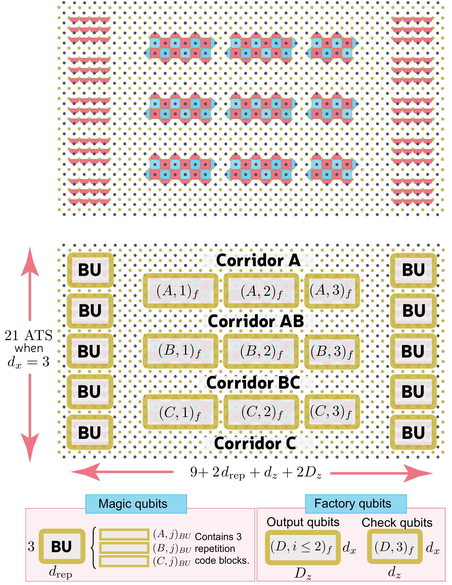
| Factory clock | Corridor A | Corridor AB | Corridor BC | Corridor C |
| 1 | ||||
| 2 | ||||
| 3 | ||||
| 4 | ||||
| 5 | ||||
| 6 | ||||
| 7 | ||||
| 8 | exit | exit | exit | exit |
O.7 Factory layout and scheduling
We see from Fig. 61 that lattice surgery require some additional workspace to connect the various codeblocks. Fig. 62 presents a 2D layout to realize TDTOF using lattice surgery, including all necessary workspace. If bit-flips are sufficiently small, then the factory can be realized completely with repetition codes. In the regime where bit-flips are rare but not completely negligible, we use a mix of repetition codeblocks (for the -qubits) and thin surface codes (for the factory qubits) to tolerate a single physical bit-flip anywhere in the factory. Additional bit-flip protection could be achieved by increasing the distance of all code blocks and/or performing two rounds of TDTOF. Here we only describe a single round and primarily focus on the version using surface code blocks.
For now, we assume a supply of TOF states generated from BUTOF. Then we can schedule the main TDTOF steps as listed in Table 13. The required 8 input are divided into 2 batches of 4. How quickly can a batch of 4 input magic states be injected? Each state comprises 3 qubits, so there are a total of multi-patch Pauli measurements needed per batch. These can be partly parallelised. Fig. 62 shows 4 horizontal empty regions that we will call access corridors labeled . This allows us to perform 4 multi-patch Pauli measurement in parallel. There are some constraints on which multi-patch Pauli measurements are performed (further discussion in the caption of Fig. 62). The first batch is injected in factory clock steps 1-3. The second batch is injected in factory clock steps 4-6. Factory clock step 7 performs the measurement of the check qubits, and starts the process of exiting some factory qubits out of the factory. Factory clock step 8 completes the process of exiting the factory qubits. Each factory clock step takes a time where is the duration of 1 surface code cycle and is the number of surface code cycle used per multi-qubit Pauli measurement. The in provides time to perform high fidelity single qubit measurements and reset between rounds of multi-qubit Pauli measurement. Roughly, a single execution of TDTOF takes time , though small extra additive timecosts may be incurred to execute BUTOF, which we discuss next.
| Fault source and remarks | Propagated | Risk | Suppressing |
| parameter | |||
| -logical errors on repetition codes during storage | Backwards | not critical | |
| -logical errors on factory qubits during storage | Forwards | critical | |
| -logical errors on check qubits during storage | Forwards | not critical | |
| logical on repetition codes during storage | Backwards | not critical | |
| logical on surface codes factory qubits | Stuck | critical | , |
| Timelike error during lattice surgery multi-patch measurement. Remarks: This flips multi-qubit measurement outcome (denoted in Algorithm 3) but is equivalent to Pauli error on input magic state. See Appendix M for details. | Backwards | not critical | |
| Measurement failure when reseting after lattice surgery. Remarks: This flips some single Pauli measurement outcome in Algorithm 3. Equivalent to Pauli error on input magic state. | Backwards | not critical |
The BUTOF protocol can have a fairly high failure probability, labeled here by . This failure probability depends on the repetition code distance used in BUTOF. To boost the probability of having ample supply of states from BUTOF, we add redundancy in both time and space. Our illustrations show modules for BUTOF, but we only need 8 input or states for the protocol. Not all 8 input or states need to exist at the same time as they are split into two batches. Rather we aim to prepare 4 at the start of factory clock steps 1 and 4. Therefore, during the factory clock steps 4-8 (a total time of ), we need to prepare 4 for the first batch of the next round of TDTOF. During the factory clock steps 1-3 (a total time of ), we need to prepare 4 for the second batch in the current round of TDTOF. Let us focus our discussion on preparation during steps 1-3 as this is the bottleneck point. Furthermore, our schedule requires that, of these 4 states, 2 are located on the left and 2 are located on the right. Considering just one side, we have BUTOF modules. Of these modules, 2 are busy storing states and performing the required lattice surgery operations. This leaves modules responsible for preparing 2 states. Each attempt at BUTOF takes a time
| (468) |
where is the optimal time for a CNOT gate and is the time for a repetition code cycle. Therefore, steps 1-3 provide enough time to fit in repeated attempts at BUTOF. Given temporally multiplexed attempts, each BUTOF module has its failure probability reduced from to . Each side fails if there are zero or one module successes of the modules, which occurs with probability
| (469) |
For instance, executing BUTOF at distance 5 and using surface code cycles per lattice surgery operation we have attempts at BUTOF (assuming and ). If then the temporal redundancy reduces this to . Providing modules in total, there is available spatial redundancy on each side, which further suppresses the failure probability to . This is already quite low. We can further reduce the failure probability by either: increasing space cost ; or inserting a small number additional rounds of BUTOF between steps 3 and 4. In the latter case, the runtime of TDTOF is extended to
| (470) |
where we have assumed . This further reduces . A coarse bound is obtained by replacing in Eq. 469, though actually the suppression is slightly better as there are now modules available for the attempts. We do not wish to set too high, as the additional delay leads to logical error accumulation due to finite distance choices.
Whenever BUTOF fails to proceed the required states, we count this as a failure of the whole TDTOF protocol. However, we use sufficient redundancy that such occurrences are very rare. Typically, we set or , and we use when and when .
An additional consideration is that a lattice dislocation is used when performing a multi-qubit Pauli measurement including a on a repetition encoded logical qubit (see Fig. 61). This dislocation uses a small amount of additional space. However, when using input states (instead of ) the third qubit differs by a Hadamard and so the protocol is adjusted to measure and a dislocation is not required. For this reason, we inject the qubits in reverse order: , then . After is injected (without needing a dislocation) some space is freed-up for dislocations to be used, enabling and to be injected.
O.8 Clifford noise
| # ATS | (%) | Time/Tof () | |||||||
| 1176 | 93 | 1602 | 5 | 5 | 7 | 15 | 3 | 11 | |
| 1218 | 73 | 1871 | 5 | 5 | 9 | 15 | 3 | 10 | |
| 1218 | 94 | 1723 | 5 | 5 | 9 | 15 | 3 | 12 | |
| 1260 | 93 | 1734 | 5 | 5 | 7 | 17 | 3 | 12 | |
| 1302 | 94 | 1724 | 5 | 5 | 9 | 17 | 3 | 12 | |
| 1386 | 98 | 1766 | 5 | 5 | 9 | 19 | 3 | 13 | |
| 1386 | 94 | 1721 | 5 | 7 | 9 | 17 | 3 | 12 | |
| 1428 | 94 | 1723 | 5 | 5 | 11 | 19 | 3 | 12 | |
| 1428 | 98 | 1889 | 5 | 5 | 11 | 19 | 3 | 14 | |
| 1470 | 98 | 1762 | 5 | 7 | 9 | 19 | 3 | 13 | |
| 1512 | 99 | 1886 | 5 | 7 | 11 | 19 | 3 | 14 | |
| 1596 | 99 | 1886 | 5 | 7 | 11 | 21 | 3 | 14 | |
| 1596 | 99 | 2137 | 5 | 7 | 11 | 21 | 3 | 16 | |
| 1680 | 99 | 2011 | 5 | 7 | 11 | 23 | 3 | 15 | |
| 1680 | 99 | 2262 | 5 | 7 | 11 | 23 | 3 | 17 | |
| 1722 | 99 | 2136 | 5 | 7 | 13 | 23 | 3 | 16 | |
| 1722 | 99 | 2388 | 5 | 7 | 13 | 23 | 3 | 18 | |
| 1806 | 99 | 2388 | 5 | 7 | 13 | 25 | 3 | 18 | |
| 1890 | 99 | 2513 | 5 | 7 | 13 | 27 | 3 | 19 | |
| 1890 | 99 | 2388 | 5 | 9 | 13 | 25 | 3 | 18 | |
| 1932 | 99 | 2388 | 5 | 7 | 15 | 27 | 3 | 18 | |
| 1932 | 99 | 2639 | 5 | 7 | 15 | 27 | 3 | 20 | |
| 1974 | 99 | 2513 | 5 | 9 | 13 | 27 | 3 | 19 | |
| 2016 | 99 | 2639 | 5 | 7 | 15 | 29 | 3 | 20 | |
| 2016 | 99 | 2388 | 5 | 9 | 15 | 27 | 3 | 18 | |
| 2016 | 99 | 2639 | 5 | 9 | 15 | 27 | 3 | 20 | |
| 2100 | 99 | 2639 | 5 | 9 | 15 | 29 | 3 | 20 | |
| 2226 | 99 | 2639 | 5 | 9 | 17 | 31 | 3 | 20 | |
| 2436 | 99 | 2639 | 5 | 9 | 19 | 35 | 3 | 20 | |
| 2604 | 99 | 2764 | 5 | 9 | 19 | 39 | 3 | 21 |
Perhaps one of the most importance aspects of magic state factory design is the choice of distance for various code blocks. It is possible to use much smaller code distances within the factory than used inside the main algorithm. Using finite code distances leads to noisy Clifford gates, noisy lattice surgery operations and non-negligible memory noise. This needs to be accounted for in addition to the error estimated by 2 under the assumption of ideal Cliffords. Indeed, typically Clifford noise is the dominate source of errors and the error of 2 should instead be regarded as the minimum achievable error (with 1 round of TDTOF) in the limit of infinite code distances.
Some of the relevant spatial code distance parameters are shown in Fig. 62. An important additional quantity is the “measurement distance” that is increased to suppress the effect of timelike errors during lattice surgery (see Appendix M for further details). A common choice in the literature is to set , but this is by no means necessary or optimal.
Rather than a Monte Carlo simulation of Clifford noise, we perform a computer-assisted analytical analysis. It is helpful to distinguish critical and non-critical faults. We say a Clifford fault is a critical risk if (assuming no other errors occur) it leads to an undetected fault on the output magic states. Conversely, a fault is a non-critical risk if it will be detected (assuming no other errors). All sources of Clifford noise can be grouped into one of four classes
- 1.
Backwards propagating and not critical: these are errors that can be commuted towards the start of the circuit, so that they act on a single noisy input state. If is the density matrix with only noise from BUTOF, the backwards propagating noise is applied so . Then the effective logical error distribution is determined from using the procedure of Section O.5.2.
- 2.
Forwards propagating and not critical: these errors can be commuted to the end of the circuit, so that they act on the check qubits in the factory just before they are measured.
- 3.
Forwards propagating and critical: these errors can be commuted to the end of the circuit, so that they act on the output magic state qubits.
- 4.
Stuck errors and potentially critical: these are errors that are difficult to commute forwards or backwards through the circuit. We sum the probability of these events and add it to the error rate on the output magic states.
Our treatment of stuck errors means that we obtain an upper bound on the performance. One might be concerned that this bound is loose, but in practice the stuck errors are very rare and not, therefore, of major importance. Indeed, if we instead attempted a Monte Carlo simulation, the statistical variance in the error estimate would exceed that of the total stuck error probability. Therefore, our computer-assisted analytical analysis leads to more accurate results than Monte Carlo methods. We further remark that while a mild amount of truncation of higher order processes is employed, we use the procedure of Section O.5.1 to monitor this truncation error and verify that it is negligible.
We list all the source of imperfections in Table 14 and describe the propagation type and risk level. Let us assume that backwards propagation has been performed and we have accounted for the effect of noise tailoring (recall Section O.6) on the error distribution. Following earlier notation of Definition 3 and Section O.6, we say noisy TOF state suffers fault with probability that we precompute. Then, without any other noise sources, 2 would describe the acceptance probability and output infidelity. However, the factory qubits may be affected by some forwarded propagated error where the labels refer to the 3 different blocks of factory qubits. We used similar notation, without the tilde, in 1 to describe how errors due to input magic states impact the protocol. To combine with the forwarded propagated errors we simply replace to add the effect of the forwarded propagated errors and follow this modification through the analysis of 2. As we did earlier, it will be useful to split to distinguish errors on check qubits and output qubits. If the forwarded propagated error on each block occurs with some probability then the results of 2 modify to
| (471) |
and
| (472) |
There are three important changes here. First, in both equations we have summed over forwards propagated errors and weighted by the appropriate probability. In the acceptance probability the summation constraint has been replaced by since to pass the check measurement any forwards propagated error must cancel (therefore equal) some other error to go undetected. Similarly, in the fidelity expression we have replaced with because to contribute to the fidelity any forwarded propagated error must cancel (therefore equal) some other error.
Calculating the expressions for , , performing the summation and adding the stuck error events is too involved to perform by hand. But it is relatively straightforward for a symbolic mathematics package such as Mathematica. Optimizing over various error suppressing parameters, we find the factory designs that achieve a certain target error per Toffoli at the minimum qubit and ATS cost (without making significant sacrifices to acceptance probabilities) and present results in Table 15.
O.9 The fidelity bottleneck in TDTOF
There are many contributing sources of error to the results presented in Tables 4 and 15. In the main text summary of Table 4, the lowest reported Toffoli error probability was . Here we discuss which error sources are the bottleneck factor that limit us from reaching higher fidelities with TDTOF protocol. We conclude with a discussion how the presented TDTOF protocol can be adapted to pass this bottleneck.
Let us consider the process of bit-flip errors on noisy input TOF states encoded in repetition codes. For hardware parameters , and , the lowest total error rate is per repetition code cycle (recall Fig. 7). If a single TOF state is stored for repetition code cycles, then roughly the accumulated error on qubits and is and this gives an additional contribution of to the non-dominate noise contributions . Returning to our benchmark example, the output error is (roughly) lower bounded by
| (473) | ||||
where is some constant that depends on the exact details of the noise profile and we have discussed examples where and . Furthermore, for the larger factory examples in Table 4 repetition codes could be in storage for as long as repetition code cycles. Together this approximate accounting indicates (with and ) that we should not expect output infidelities lower than . Of course, this is a rough estimation of one error source, just to provide the reader with some intuition. Rather, for a precise accounting of all error sources the lowest observed infidelity was . However, there are several straightforward routes to reaching even lower infidelities. By converting immediately after BUTOF from repetition code to thin surface code we would reduce the time exposed to bit-flip errors. For our benchmark example, encoding directly into surface codes should enable us to get much closer to infidelity (the ideal Clifford limit for noise tailored TDTOF). Ultimately, arbitrarily high fidelities can be reached by concatenating TDTOF, though resource costs jump substantially with each level of concatenation. Alternatively, better fidelities could be reached it hardware parameters could be improved by either further suppressing bit-flips by increasing or decreasing .
References
- Bravyi and Kitaev (1998) S. B. Bravyi and A. Y. Kitaev, arXiv preprint quant-ph/9811052 (1998).
- O’Gorman and Campbell (2017) J. O’Gorman and E. T. Campbell, Physical Review A 95, 032338 (2017), arXiv:1605.07197 .
- Motta et al. (2018) M. Motta, E. Ye, J. R. McClean, Z. Li, A. J. Minnich, R. Babbush, and G. K.-L. Chan, Low rank representations for quantum simulation of electronic structure (2018), arXiv:1808.02625 .
- Gidney and Ekerå (2019) C. Gidney and M. Ekerå, How to factor 2048 bit RSA integers in 8 hours using 20 million noisy qubits (2019), arXiv:1905.09749 [quant-ph] .
- Campbell et al. (2019) E. Campbell, A. Khurana, and A. Montanaro, Quantum 3, 167 (2019), arXiv:1810.05582 .
- Kivlichan et al. (2020) I. D. Kivlichan, C. Gidney, D. W. Berry, N. Wiebe, J. McClean, W. Sun, Z. Jiang, N. Rubin, A. Fowler, A. Aspuru-Guzik, and et al., Quantum 4, 296 (2020), arXiv:1902.10673 .
- Chamberland and Campbell (2021) C. Chamberland and E. T. Campbell, arXiv preprint arXiv:2109.02746 (2021).
- Tuckett et al. (2018) D. K. Tuckett, S. D. Bartlett, and S. T. Flammia, Phys. Rev. Lett. 120, 050505 (2018), arXiv:1708.08474 .
- Tuckett et al. (2019) D. K. Tuckett, A. S. Darmawan, C. T. Chubb, S. Bravyi, S. D. Bartlett, and S. T. Flammia, Phys. Rev. X 9, 041031 (2019), arXiv:1812.08186 .
- Tuckett et al. (2020) D. K. Tuckett, S. D. Bartlett, S. T. Flammia, and B. J. Brown, Phys. Rev. Lett. 124, 130501 (2020), arXiv:1907.02554 .
- Ataides et al. (2021) J. P. B. Ataides, D. K. Tuckett, S. D. Bartlett, S. T. Flammia, and B. J. Brown, Nature communications 12, 1 (2021).
- Aliferis and Preskill (2008) P. Aliferis and J. Preskill, Phys. Rev. A 78, 052331 (2008), arXiv:0710.1301 .
- Puri et al. (2020) S. Puri, L. St-Jean, J. A. Gross, A. Grimm, N. E. Frattini, P. S. Iyer, A. Krishna, S. Touzard, L. Jiang, A. Blais, and et al., Science Advances 6, eaay5901 (2020), arXiv:1905.00450 .
- Guillaud and Mirrahimi (2019) J. Guillaud and M. Mirrahimi, Phys. Rev. X 9, 041053 (2019), arXiv:1904.09474 .
- Guillaud and Mirrahimi (2021) J. Guillaud and M. Mirrahimi, Phys. Rev. A 103, 042413 (2021).
- Mirrahimi et al. (2014) M. Mirrahimi, Z. Leghtas, V. V. Albert, S. Touzard, R. J. Schoelkopf, L. Jiang, and M. H. Devoret, New Journal of Physics 16, 045014 (2014).
- Puri et al. (2017) S. Puri, S. Boutin, and A. Blais, npj Quantum Inf. 3, 18 (2017).
- Cohen (2017) J. Cohen, Autonomous quantum error correction with superconducting qubits, Ph.D. thesis, Université Paris sciences et lettres (2017).
- Albert et al. (2018) V. V. Albert, K. Noh, K. Duivenvoorden, D. J. Young, R. T. Brierley, P. Reinhold, C. Vuillot, L. Li, C. Shen, S. M. Girvin, B. M. Terhal, and L. Jiang, Phys. Rev. A 97, 032346 (2018).
- Joshi et al. (2020) A. Joshi, K. Noh, and Y. Y. Gao, arXiv e-prints , arXiv:2008.13471 (2020), arXiv:2008.13471 [quant-ph] .
- Cai et al. (2020) W. Cai, Y. Ma, W. Wang, C. L. Zou, and L. Sun, arXiv e-prints , arXiv:2010.08699 (2020), arXiv:2010.08699 [quant-ph] .
- Leghtas et al. (2015) Z. Leghtas, S. Touzard, I. M. Pop, A. Kou, B. Vlastakis, A. Petrenko, K. M. Sliwa, A. Narla, S. Shankar, M. J. Hatridge, M. Reagor, L. Frunzio, R. J. Schoelkopf, M. Mirrahimi, and M. H. Devoret, Science 347, 853 (2015), 1412.4633 .
- Touzard et al. (2018) S. Touzard, A. Grimm, Z. Leghtas, S. Mundhada, P. Reinhold, C. Axline, M. Reagor, K. Chou, J. Blumoff, K. Sliwa, and et al., Physical Review X 8, 021005 (2018), arXiv:1705.02401 .
- Goto (2016a) H. Goto, Scientific Reports 6, 21686 (2016a).
- Goto (2016b) H. Goto, Phys. Rev. A 93, 050301 (2016b).
- Puri et al. (2019) S. Puri, A. Grimm, P. Campagne-Ibarcq, A. Eickbusch, K. Noh, G. Roberts, L. Jiang, M. Mirrahimi, M. H. Devoret, and S. M. Girvin, Phys. Rev. X 9, 041009 (2019).
- Grimm et al. (2020) A. Grimm, N. E. Frattini, S. Puri, S. O. Mundhada, S. Touzard, M. Mirrahimi, S. M. Girvin, S. Shankar, and M. H. Devoret, Nature 584, 205 (2020), arXiv:1907.12131 .
- Lescanne et al. (2020) R. Lescanne, M. Villiers, T. Peronnin, A. Sarlette, M. Delbecq, B. Huard, T. Kontos, M. Mirrahimi, and Z. Leghtas, Nature Physics 16, 509 (2020).
- Arrangoiz-Arriola and Safavi-Naeini (2016) P. Arrangoiz-Arriola and A. H. Safavi-Naeini, Phys. Rev. A 94, 063864 (2016).
- MacCabe et al. (2020) G. S. MacCabe, H. Ren, J. Luo, J. D. Cohen, H. Zhou, A. Sipahigil, M. Mirhosseini, and O. Painter, Science 370, 840 (2020), https://science.sciencemag.org/content/370/6518/840.full.pdf .
- Blais et al. (2021) A. Blais, A. L. Grimsmo, S. M. Girvin, and A. Wallraff, Rev. Mod. Phys. 93, 025005 (2021).
- Arrangoiz-Arriola et al. (2019) P. Arrangoiz-Arriola, E. A. Wollack, Z. Wang, M. Pechal, W. Jiang, T. P. McKenna, J. D. Witmer, R. Van Laer, and A. H. Safavi-Naeini, Nature 571, 537 (2019).
- Dennis et al. (2002a) E. Dennis, A. Kitaev, A. Landahl, and J. Preskill, Journal of Mathematical Physics 43, 4452 (2002a).
- Fowler et al. (2012a) A. G. Fowler, M. Mariantoni, J. M. Martinis, and A. N. Cleland, Physical Review A 86, 032324 (2012a).
- Wollack et al. (2021) E. A. Wollack, A. Y. Cleland, P. Arrangoiz-Arriola, T. P. McKenna, R. G. Gruenke, R. N. Patel, W. Jiang, C. J. Sarabalis, and A. H. Safavi-Naeini, Applied Physics Letters 118, 123501 (2021), https://doi.org/10.1063/5.0034909 .
- Campbell et al. (2017) E. T. Campbell, B. M. Terhal, and C. Vuillot, Nature 549, 172 (2017).
- Bravyi and Haah (2012) S. Bravyi and J. Haah, Phys. Rev. A 86, 052329 (2012).
- Meier et al. (2013) A. M. Meier, B. Eastin, and E. Knill, Quant. Inf. and Comp. 13, 195 (2013).
- Campbell and Howard (2018) E. T. Campbell and M. Howard, Quantum 2, 56 (2018).
- Bravyi and Kitaev (2005a) S. Bravyi and A. Kitaev, Phys. Rev. A 71, 022316 (2005a).
- Paz and Zurek (1998) J. P. Paz and W. H. Zurek, Proceedings of the Royal Society of London. Series A: Mathematical, Physical and Engineering Sciences 454, 355 (1998).
- Ahn et al. (2002) C. Ahn, A. C. Doherty, and A. J. Landahl, Phys. Rev. A 65, 042301 (2002).
- Sarovar and Milburn (2005) M. Sarovar and G. J. Milburn, Phys. Rev. A 72, 012306 (2005).
- Kerckhoff et al. (2010) J. Kerckhoff, H. I. Nurdin, D. S. Pavlichin, and H. Mabuchi, Physical Review Letters 105, 040502 (2010).
- Cochrane et al. (1999) P. T. Cochrane, G. J. Milburn, and W. J. Munro, Phys. Rev. A 59, 2631 (1999).
- Jeong and Kim (2002) H. Jeong and M. S. Kim, Phys. Rev. A 65, 042305 (2002).
- Lieu et al. (2020) S. Lieu, R. Belyansky, J. T. Young, R. Lundgren, V. V. Albert, and A. V. Gorshkov, Physical Review Letters 125, 10.1103/physrevlett.125.240405 (2020).
- Reiter and Sørensen (2012) F. Reiter and A. S. Sørensen, Phys. Rev. A 85, 032111 (2012).
- Frattini et al. (2017) N. E. Frattini, U. Vool, S. Shankar, A. Narla, K. M. Sliwa, and M. H. Devoret, Applied Physics Letters 110, 222603 (2017), https://doi.org/10.1063/1.4984142 .
- Mirhosseini et al. (2020) M. Mirhosseini, A. Sipahigil, M. Kalaee, and O. Painter, arXiv preprint arXiv:2004.04838 (2020).
- Lescanne et al. (2019) R. Lescanne, L. Verney, Q. Ficheux, M. H. Devoret, B. Huard, M. Mirrahimi, and Z. Leghtas, Phys. Rev. Applied 11, 014030 (2019).
- Sank et al. (2016) D. Sank, Z. Chen, M. Khezri, J. Kelly, R. Barends, B. Campbell, Y. Chen, B. Chiaro, A. Dunsworth, A. Fowler, E. Jeffrey, E. Lucero, A. Megrant, J. Mutus, M. Neeley, C. Neill, P. J. J. O’Malley, C. Quintana, P. Roushan, A. Vainsencher, T. White, J. Wenner, A. N. Korotkov, and J. M. Martinis, Phys. Rev. Lett. 117, 190503 (2016).
- Zhang et al. (2019) Y. Zhang, B. J. Lester, Y. Y. Gao, L. Jiang, R. J. Schoelkopf, and S. M. Girvin, Phys. Rev. A 99, 012314 (2019).
- Verney et al. (2019) L. Verney, R. Lescanne, M. H. Devoret, Z. Leghtas, and M. Mirrahimi, Phys. Rev. Applied 11, 024003 (2019).
- James and Jerke (2007a) D. F. V. James and J. Jerke, Can. J. Phys. 85, 625 (2007a).
- Gamel and James (2010) O. Gamel and D. F. V. James, Phys. Rev. A 82, 052106 (2010).
- Naik et al. (2017) R. K. Naik, N. Leung, S. Chakram, P. Groszkowski, Y. Lu, N. Earnest, D. C. McKay, J. Koch, and D. I. Schuster, Nat. Commun. 8, 1904 (2017).
- Pechal et al. (2018) M. Pechal, P. Arrangoiz-Arriola, and A. H. Safavi-Naeini, Quantum Sci. Technol. 4, 015006 (2018).
- Hann et al. (2019) C. T. Hann, C.-L. Zou, Y. Zhang, Y. Chu, R. J. Schoelkopf, S. M. Girvin, and L. Jiang, Phys. Rev. Lett. 123, 250501 (2019).
- Mundada et al. (2019) P. Mundada, G. Zhang, T. Hazard, and A. Houck, Phys. Rev. Appl. 12, 10.1103/PhysRevApplied.12.054023 (2019).
- Chen et al. (2014) Y. Chen, C. Neill, P. Roushan, N. Leung, M. Fang, R. Barends, J. Kelly, B. Campbell, Z. Chen, B. Chiaro, A. Dunsworth, E. Jeffrey, A. Megrant, J. Y. Mutus, P. J. J. O’Malley, C. M. Quintana, D. Sank, A. Vainsencher, J. Wenner, T. C. White, M. R. Geller, A. N. Cleland, and J. M. Martinis, Phys. Rev. Lett. 113, 220502 (2014).
- Gao et al. (2018) Y. Y. Gao, B. J. Lester, Y. Zhang, C. Wang, S. Rosenblum, L. Frunzio, L. Jiang, S. M. Girvin, and R. J. Schoelkopf, Phys. Rev. X 8, 021073 (2018).
- Gao et al. (2019) Y. Y. Gao, B. J. Lester, K. S. Chou, L. Frunzio, M. H. Devoret, L. Jiang, S. M. Girvin, and R. J. Schoelkopf, Nature 566, 509 (2019).
- Sun et al. (2014) L. Sun, A. Petrenko, Z. Leghtas, B. Vlastakis, G. Kirchmair, K. Sliwa, A. Narla, M. Hatridge, S. Shankar, J. Blumoff, et al., Nature 511, 444 (2014).
- Hann et al. (2018) C. T. Hann, S. S. Elder, C. S. Wang, K. Chou, R. J. Schoelkopf, and L. Jiang, Phys. Rev. A 98, 022305 (2018).
- Elder et al. (2020) S. S. Elder, C. S. Wang, P. Reinhold, C. T. Hann, K. S. Chou, B. J. Lester, S. Rosenblum, L. Frunzio, L. Jiang, and R. J. Schoelkopf, Phys. Rev. X 10, 011001 (2020).
- Krantz et al. (2019) P. Krantz, M. Kjaergaard, F. Yan, T. P. Orlando, S. Gustavsson, and W. D. Oliver, Applied Physics Reviews 6, 021318 (2019).
- Gottesman (2010) D. Gottesman, Proceedings of Symposia in Applied Mathematics 68, 13 (2010).
- Tomita and Svore (2014) Y. Tomita and K. M. Svore, Phys. Rev. A 90, 062320 (2014).
- DiVincenzo and Aliferis (2007) D. P. DiVincenzo and P. Aliferis, Phys. Rev. Lett. 98, 020501 (2007).
- Chamberland et al. (2018) C. Chamberland, P. Iyer, and D. Poulin, Quantum 2, 43 (2018).
- Kelly et al. (2015) J. Kelly, R. Barends, A. G. Fowler, A. Megrant, E. Jeffrey, T. C. White, D. Sank, J. Y. Mutus, B. Campbell, Y. Chen, et al., Nature 519, 66 (2015).
- Ballance et al. (2016) C. J. Ballance, T. P. Harty, N. M. Linke, M. A. Sepiol, and D. M. Lucas, Phys. Rev. Lett. 117, 060504 (2016).
- Sung et al. (2021) Y. Sung, L. Ding, J. Braumüller, A. Vepsäläinen, B. Kannan, M. Kjaergaard, A. Greene, G. O. Samach, C. McNally, D. Kim, A. Melville, B. M. Niedzielski, M. E. Schwartz, J. L. Yoder, T. P. Orlando, S. Gustavsson, and W. D. Oliver, Phys. Rev. X 11, 021058 (2021).
- Fowler et al. (2013) A. G. Fowler, S. J. Devitt, and C. Jones, Scientific reports 3, 1 (2013).
- Horsman et al. (2012) C. Horsman, A. G. Fowler, S. Devitt, and R. V. Meter, New Journal of Physics 14, 123011 (2012).
- Landahl and Ryan-Anderson (2014) A. J. Landahl and C. Ryan-Anderson, arXiv preprint arXiv:1407.5103 (2014).
- Litinski and Oppen (2018) D. Litinski and F. v. Oppen, Quantum 2, 62 (2018).
- Litinski (2019a) D. Litinski, Quantum 3, 128 (2019a).
- Litinski and von Oppen (2018) D. Litinski and F. von Oppen, Quantum 2, 62 (2018).
- Bravyi et al. (2016) S. Bravyi, G. Smith, and J. A. Smolin, Physical Review X 6, 021043 (2016).
- Paler and Fowler (2019) A. Paler and A. G. Fowler, arXiv preprint arXiv:1906.07994 (2019).
- Fowler et al. (2012b) A. G. Fowler, M. Mariantoni, J. M. Martinis, and A. N. Cleland, Phys. Rev. A 86, 032324 (2012b).
- Fowler (2012a) A. G. Fowler, arXiv preprint arXiv:1210.4626 (2012a).
- Chamberland and Cross (2019) C. Chamberland and A. W. Cross, Quantum 3, 143 (2019).
- Chamberland and Noh (2020) C. Chamberland and K. Noh, npj Quantum Information 6, 91 (2020).
- (87) Recently, it was also shown in Ref. Guillaud and Mirrahimi 2021 that when implementing a logical Toffoli gate using a piece-wise fault-tolerant approach, one can track the errors that arise when errors propagate through the target qubits of the physical Toffoli gates (see Appendix L) and correct all errors at the final output of piece-wise circuit (instead of in between each blocks of physical Toffoli gates). Such an approach could potentially be used in our bottom-up state preparation scheme, allowing us to avoid using the STOP algorithm to prepare and . However we leave such an analysis to future work.
- (88) This should be compared to the circuits used in Chamberland and Noh 2020 for preparing type magic states which are fault-tolerant to all types of Pauli noise given that a depolarizing circuit level noise model was assumed.
- Bravyi and Kitaev (2005b) S. Bravyi and A. Kitaev, Phys. Rev. A 71, 022316 (2005b).
- Haah and Hastings (2018) J. Haah and M. B. Hastings, Quantum 2, 71 (2018).
- Litinski (2019b) D. Litinski, Quantum 3, 205 (2019b).
- Gidney and Fowler (2019) C. Gidney and A. G. Fowler, Quantum 3, 135 (2019).
- Wiebe and Granade (2016) N. Wiebe and C. Granade, Phys. Rev. Lett. 117, 010503 (2016).
- Gidney (2018) C. Gidney, Quantum 2, 74 (2018).
- Bravyi et al. (2019) S. Bravyi, D. Browne, P. Calpin, E. Campbell, D. Gosset, and M. Howard, Quantum 3, 181 (2019).
- Campbell (2020) E. Campbell (2020), arXiv:2012.09238.
- Zheng et al. (2017) B.-X. Zheng, C.-M. Chung, P. Corboz, G. Ehlers, M.-P. Qin, R. M. Noack, H. Shi, S. R. White, S. Zhang, and G. K.-L. Chan, Science 358, 1155 (2017).
- (98) In contract, for an additive (intensive) error energy estimation, is constant in , and so the gate complexity will grow with system size Kivlichan et al. 2020; Campbell 2020.
- Li et al. (2019) M. Li, D. Miller, M. Newman, Y. Wu, and K. R. Brown, Phys. Rev. X 9, 021041 (2019).
- Chamberland et al. (2020a) C. Chamberland, G. Zhu, T. J. Yoder, J. B. Hertzberg, and A. W. Cross, Phys. Rev. X 10, 011022 (2020a).
- Debroy et al. (2020) D. M. Debroy, M. Li, S. Huang, and K. R. Brown, Quantum Science and Technology 5, 034002 (2020).
- Huang and Brown (2020) S. Huang and K. R. Brown, Phys. Rev. A 101, 042312 (2020).
- Nigg et al. (2012) S. E. Nigg, H. Paik, B. Vlastakis, G. Kirchmair, S. Shankar, L. Frunzio, M. H. Devoret, R. J. Schoelkopf, and S. M. Girvin, Phys. Rev. Lett. 108, 240502 (2012).
- Pechal and Safavi-Naeini (2017) M. Pechal and A. H. Safavi-Naeini, Phys. Rev. A 96, 042305 (2017).
- Kreikebaum et al. (2020) J. M. Kreikebaum, K. P. O’Brien, A. Morvan, and I. Siddiqi, Superconductor Science and Technology 33, 06LT02 (2020).
- Ferreira et al. (2020) V. S. Ferreira, J. Banker, A. Sipahigil, M. H. Matheny, A. J. Keller, E. Kim, M. Mirhosseini, and O. Painter, arXiv preprint arXiv:2001.03240 (2020).
- Azouit et al. (2016) R. Azouit, A. Sarlette, and P. Rouchon, in 2016 IEEE 55th Conference on Decision and Control (CDC) (IEEE, 2016) pp. 4559–4565.
- Azouit et al. (2017) R. Azouit, F. Chittaro, A. Sarlette, and P. Rouchon, Quantum Sci. Technol. 2, 044011 (2017).
- Sete et al. (2015) E. A. Sete, J. M. Martinis, and A. N. Korotkov, Phys. Rev. A 92, 012325 (2015).
- James and Jerke (2007b) D. F. James and J. Jerke, Canadian Journal of Physics 85, 625 (2007b), https://doi.org/10.1139/p07-060 .
- Heinsoo et al. (2018) J. Heinsoo, C. K. Andersen, A. Remm, S. Krinner, T. Walter, Y. Salathé, S. Gasparinetti, J.-C. Besse, A. Potočnik, A. Wallraff, and C. Eichler, Phys. Rev. Applied 10, 034040 (2018).
- Jeffrey et al. (2014) E. Jeffrey, D. Sank, J. Y. Mutus, T. C. White, J. Kelly, R. Barends, Y. Chen, Z. Chen, B. Chiaro, A. Dunsworth, A. Megrant, P. J. J. O’Malley, C. Neill, P. Roushan, A. Vainsencher, J. Wenner, A. N. Cleland, and J. M. Martinis, Phys. Rev. Lett. 112, 190504 (2014).
- Pfaff et al. (2017) W. Pfaff, C. Axline, L. Burkhart, et al., Nature Physics 13, 882 (2017).
- Clerk et al. (2010) A. A. Clerk, M. H. Devoret, S. M. Girvin, F. Marquardt, and R. J. Schoelkopf, Rev. Mod. Phys. 82, 1155 (2010).
- Didier et al. (2015) N. Didier, J. Bourassa, and A. Blais, Phys. Rev. Lett. 115, 203601 (2015).
- Chamberland and Beverland (2018) C. Chamberland and M. E. Beverland, Quantum 2, 53 (2018).
- Aliferis et al. (2006) P. Aliferis, D. Gottesman, and J. Preskill, Quantum Info. Comput. 6, 97 (2006).
- Edmonds (1965) J. Edmonds, Canadian Journal of mathematics 17, 449 (1965).
- Delfosse and Nickerson (2017) N. Delfosse and N. H. Nickerson, arXiv e-prints , arXiv:1709.06218 (2017), arXiv:1709.06218 .
- (120) There are cases where families of error correcting codes have thresholds when using the STOP algorithm to decode with the syndrome from the last round. One such example includes concatenated codes using the methods of Aliferis et al. 2006.
- Brooks and Preskill (2013) P. Brooks and J. Preskill, Physical Review A 87, 032310 (2013).
- Anderson et al. (2014) J. T. Anderson, G. Duclos-Cianci, and D. Poulin, Phys. Rev. Lett. 113, 080501 (2014).
- Vuillot et al. (2019) C. Vuillot, L. Lao, B. Criger, C. G. Almudéver, K. Bertels, and B. M. Terhal, New Journal of Physics 21, 033028 (2019).
- Landahl and Ryan-Anderson (2014) A. J. Landahl and C. Ryan-Anderson, arXiv e-prints , arXiv:1407.5103 (2014), arXiv:1407.5103 .
- G. Fowler and Gidney (2018) A. G. Fowler and C. Gidney, arXiv:1808.06709 (2018).
- Gottesman (1999) D. Gottesman, Proceedings, XXII International Colloquium on Group Theoretical Methods in Physics , 32 (1999).
- Dennis et al. (2002b) E. Dennis, A. Kitaev, A. Landahl, and J. Preskill, J. Math. Phys. 43, 4452 (2002b).
- Kovalev and Pryadko (2012) A. A. Kovalev and L. P. Pryadko, arXiv preprint arXiv:1208.2317 (2012).
- Raussendorf and Harrington (2007) R. Raussendorf and J. Harrington, Physical review letters 98, 190504 (2007).
- Wang et al. (2011) D. S. Wang, A. G. Fowler, and L. C. L. Hollenberg, Phys. Rev. A 83, 020302 (2011).
- Fowler (2012b) A. G. Fowler, Phys. Rev. Lett. 109, 180502 (2012b).
- Chamberland et al. (2020b) C. Chamberland, A. Kubica, T. J. Yoder, and G. Zhu, New Journal of Physics 22, 023019 (2020b).
- Shor (1996) P. W. Shor, in Proceedings of the 37th Annual Symposium on Foundations of Computer Science, FOCS ’96 (IEEE Computer Society, USA, 1996) p. 56.
- Dennis (2001) E. Dennis, Phys. Rev. A 63, 052314 (2001).
- Jones (2013a) C. Jones, Phys. Rev. A 87, 042305 (2013a).
- Fowler (2013) A. G. Fowler, arXiv:1310.0863 (2013).
- Hastings and Haah (2018) M. B. Hastings and J. Haah, Physical review letters 120, 050504 (2018).
- Jones (2013b) C. Jones, Phys. Rev. A. 87, 022328 (2013b).
- Eastin (2013) B. Eastin, Phys. Rev. A. 87, 032321 (2013).
- Campbell and O’Gorman (2016) E. T. Campbell and J. O’Gorman, Quantum Science and Technology 1, 015007 (2016).
- Campbell and Howard (2017a) E. T. Campbell and M. Howard, Physical Review A 95, 022316 (2017a).
- Campbell and Howard (2017b) E. T. Campbell and M. Howard, Physical review letters 118, 060501 (2017b).
- Haah et al. (2017) J. Haah, M. B. Hastings, D. Poulin, and D. Wecker, Quantum 1, 31 (2017).
- Paetznick and Reichardt (2013) A. Paetznick and B. W. Reichardt, Physical review letters 111, 090505 (2013).
- Kubica et al. (2015) A. Kubica, B. Yoshida, and F. Pastawski, New Journal of Physics 17, 083026 (2015).
- Vasmer and Browne (2018) M. Vasmer and D. E. Browne, arXiv preprint arXiv:1801.04255 (2018).
- MacWilliams and Sloane (1988) F. MacWilliams and N. Sloane, The Theory of Error-Correcting Codes (North Holland, 1988).