跳到论文正文
W Papers独立论文阅读器 arXiv:2012.04076 论文正文 计算阅读时间 · 0%
引用这篇论文根据当前论文元数据生成,正式投稿前建议核对。


License: arXiv.org perpetual non-exclusive license
arXiv:2012.04076v1 [math.PR] 07 Dec 2020

Undirected Polymers in Random Environment:
path properties in the mean field limit.Thanks: We are indebted to Lisa Hartung and Marius A. Schmidt for helpful conversations. This work has been partially supported by a DFG research grant, contract number 2337/1-1.

Nicola Kistler Address: Nicola Kistler
J.W. Goethe-Universität Frankfurt, Germany.
Email address: kistler@math.uni-frankfurt.de
and Adrien Schertzer Address: adrien schertzer
J.W. Goethe-Universität Frankfurt, Germany.
Email address: schertzer@math.uni-frankfurt.de
Date: August 11, 2026
Abstract.

We consider the problem of undirected polymers (tied at the endpoints) in random environment, also known as the unoriented first passage percolation on the hypercube, in the limit of large dimensions. By means of the multiscale refinement of the second moment method we obtain a fairly precise geometrical description of optimal paths, i.e. of polymers with minimal energy. The picture which emerges can be loosely summarized as follows. The energy of the polymer is, to first approximation, uniformly spread along the strand. The polymer’s bonds carry however a lower energy than in the directed setting, and are reached through the following geometrical evolution. Close to the origin, the polymer proceeds in oriented fashion – it is thus as stretched as possible. The tension of the strand decreases however gradually, with the polymer allowing for more and more backsteps as it enters the core of the hypercube. Backsteps, although increasing the length of the strand, allow the polymer to connect reservoirs of energetically favorable edges which are otherwise unattainable in a fully directed regime. These reservoirs lie at mesoscopic distance apart, but in virtue of the high dimensional nature of the ambient space, the polymer manages to connect them through approximate geodesics with respect to the Hamming metric: this is the key strategy which leads to an optimal energy/entropy balance. Around halfway, the mirror picture sets in: the polymer tension gradually builds up again, until full orientedness close to the endpoint. The approach yields, as a corollary, a constructive proof of the result by Martinsson [Ann. Appl. Prob. 26 (2016), Ann. Prob. 46 (2018)] concerning the leading order of the ground state.

Key words and phrases: 
Undirected polymers in random environment, first passage percolation, hypercube, mean field limits.
2000 Mathematics Subject Classification
60J80, 60G70, 82B44

In memory of Dima Ioffe.

1. Introduction

We denote by Gn=(Vn,En)G_{n}=(V_{n},E_{n}) the nn-dimensional hypercube. Vn={0,1}nV_{n}=\{0,1\}^{n} is thus the set of vertices, and EnE_{n} the set of edges connecting nearest neighbours. We write 𝟎=(0,0,…,0)\boldsymbol{0}=(0,0,...,0) and 𝟏=(1,1,…,1){\boldsymbol{1}}=(1,1,...,1) for diametrically opposite vertices. For l∈ℕl\in\mathbb{N} we let

Π~n,l≡the set of polymers, i.e. paths from 0 to 1 of lengthl,\widetilde{\Pi}_{n,l}\equiv\text{the set of polymers, i.e. paths from {0} to {1} of length}\;l\,,

as well as

Π~n≡⋃l=1∞Π~n,l.\widetilde{\Pi}_{n}\equiv\bigcup\limits_{l=1}^{\infty}\widetilde{\Pi}_{n,l}.

For π∈Π~n\pi\in\tilde{\Pi}_{n} a polymer going through two vertices 𝒗,𝒘\boldsymbol{v},\boldsymbol{w} of the hypercube, we denote by lπ​(𝒗,𝒘)l_{\pi}(\boldsymbol{v},\boldsymbol{w}) the length of the connecting substrand, also shortening lπ≡lπ​(𝟎,𝟏)l_{\pi}\equiv l_{\pi}(\boldsymbol{0},\boldsymbol{1}).

Every edge of the nn-hypercube is parallel to some unit vector ej∈ℝne_{j}\in\mathbb{R}^{n}, where eje_{j} connects

(0,…,0)​and​(0,…,0,1⏟jt​h−coordinate,0,…,0).(0,\dots,0)\;\text{and}\;(0,\dots,0,\underbrace{1}_{j^{th}-\text{coordinate}},0,\dots,0)\,.

We write e−j≡−eje_{-j}\equiv-e_{j}. The quantity πj∈{1,n}∪{−1,−n}\pi_{j}\in\{1,n\}\cup\{-1,-n\} then specifies the direction of a π\pi-path at step jj. A forward step occurs if πj∈{1,n}\pi_{j}\in\{1,n\}; if πj∈{−1,−n}\pi_{j}\in\{-1,-n\} we refer to this as a backstep.

Remark that the endpoint of the (sub)path π1​π2​…​πi\pi_{1}\pi_{2}\dots\pi_{i} coincides with the vertex given by ∑j≤ieπj\sum_{j\leq i}{e_{\pi_{j}}}. The edge traversed in the jj-th step by the π\pi-path will be denoted [π]j[\pi]_{j}.

To each edge we attach independent, standard (mean one) exponentials random variables ξ\xi, the random environment, and assign to a polymer π∈Π~n,l\pi\in\widetilde{\Pi}_{n,l} its weight/energy according to

Xπ≡∑j=1lξ[π]j.X_{\pi}\equiv\sum_{j=1}^{l}\xi_{[\pi]_{j}}.

The question we wish to address concerns the ground state of undirected polymers in random environment11 1 This problem also appears in the literature under the name of unoriented first passage percolation, FPP for short. In mathematical biology it bears relevance to the issue of fitness landscapes. in which case it is dubbed accessibility percolation, see [1, 2, 6, 12, 13, 14, 10, 11] and references therein. We adopt here the polymer terminology since it is arguably more suitable to convey the type of results we obtain., to wit:

mn≡minπ∈Π~n⁡Xπ,m_{n}\equiv\min_{{\pi}\in\widetilde{\Pi}_{n}}X_{\pi}, (1.1)

in the mean field limit n↑∞n\uparrow\infty, and the statistical/geometrical properties of optimal paths.

A first remark is in place: since polymers with loops cannot achieve the ground state (their energy can always be reduced by removing the loops), we will henceforth focus on the set of loopless paths of length l∈ℕl\in\mathbb{N}, denoted Πn,l\Pi_{n,l}, and shortening, in full analogy,

Πn≡⋃l=1∞Πn,l,\Pi_{n}\equiv\bigcup\limits_{l=1}^{\infty}\Pi_{n,l},

for the set of all loopless paths.

Looplessness will be very useful: it guarantees, in particular, that the energy of a polymer of length, say, ll, is indeed given by the sum of ll independent standard exponentials. On the other hand, loopless paths are not necessarily directed, see Figure 1 below for a graphical rendition.

Refer to caption
Figure 1. The 10-dim hypercube with two polymers. The blue polymer is directed: its length coincides with the dimension (l=n=10l=n=10), and it is thus as stretched as possible. The red polymer is undirected: it performs backsteps, which account for a lower ”tension”, and for the long excursions (l=20l=20).

It is clear that a major issue here will be that of path counting. For the hypercube, the following beautiful formula is available. We denote by Mn,l,dM_{n,l,d} the number of polymers of length ll between two points at Hamming distance dd, i.e. points thus disagree in exactly dd coordinates. It then holds :

Mn,l,d=12n​∑i=0n∑j=0d(dj)​(n−di−j)​(−1)j​(n−2​i)l​𝟙j≤i.\displaystyle M_{n,l,d}=\frac{1}{2^{n}}\sum_{i=0}^{n}\sum_{j=0}^{d}\binom{d}{j}\binom{n-d}{i-j}{(-1)}^{j}{(n-2i)}^{l}\mathbbm{1}_{j\leq i}. (1.2)

(This formula concerns all paths of given length: loops, in particular, are also allowed). A proof of this formula, which relies on the classical approach via adjancency matrices, can be found in the monograph by Stanley [15]. Since we were not able to identify its first discoverer, we will refer to (1.2) as Stanley’s formula.

No less remarkable is the following Stanley’s identity, relating Mn,l,dM_{n,l,d} to hyperbolic functions. For x∈ℝx\in\mathbb{R}, it holds:

∑l=0∞Mn,l,dxll!=sinh(x)dcosh(x)n−d.\displaystyle\sum_{l=0}^{\infty}M_{n,l,d}\frac{x^{l}}{l!}={\sinh(x)}^{d}{\cosh(x)}^{n-d}\,. (1.3)

Assuming the validity of (1.2), the proof of (1.3) only requires the binomial theorem and elementary Taylor expansions: it will be given in the Appendix for completeness. Lightening notations further by setting Mn,l≡Mn,l,nM_{n,l}\equiv M_{n,l,n} for the number of polymers of length ll between two opposite vertices on the hypercube, it thus follows from (1.3) that

∑l=0∞Mn,l​xll!=sinh⁡(x)n.\sum_{l=0}^{\infty}M_{n,l}\frac{x^{l}}{l!}={\sinh(x)}^{n}\,. (1.4)

This relation will allow for precise asymptotical analysis. Before seeing a first, key application, we shall recall yet another technical input concerning tail estimates for the distribution of the sum of independent standard exponentials as appearing in the problem at hand: denoting by {ξi}i∈ℕ\{\xi_{i}\}_{i\in\mathbb{N}} a family of such random variables and with Xl≡∑i≤lξiX_{l}\equiv\sum_{i\leq l}\xi_{i}, it then holds:

ℙ⁡(Xl≤x)=(1+K⁡(x,l))​e−x​xll!,\mathbb{P}\left(X_{l}\leq x\right)=\left(1+K(x,l)\right)\frac{e^{-x}x^{l}}{l!}, (1.5)

for x>0x>0, and with 0≤K⁡(x,l)≤ex​x/(l+1).0\leq K(x,l)\leq e^{x}x/(l+1). (The proof is truly elementary, but see e.g. [8, Lemma 5] for details).

Some notational convention: for an,bn≥0a_{n},b_{n}\geq 0 we write an≲bna_{n}\lesssim b_{n} if an≤C​bna_{n}\leq Cb_{n} for some numerical constant C>0C>0 and an∝bna_{n}\propto b_{n} if an≲bna_{n}\lesssim b_{n} and bn≲anb_{n}\lesssim a_{n} .

Armed with Stanley’s formula and the tail estimates, we are now ready to make the aforementioned key observation concerning the ground state of undirected polymers: denoting by Nn,l,x≡#⁡{π∈Πn,l,Xπ≤x}N_{n,l,x}\equiv\#\{\pi\in\Pi_{n,l},X_{\pi}\leq x\} the number of polymers of length ll and energies at most xx, by union bounds and Markov inequality we have

ℙ(mn≤x)=ℙ(∪l=0∞{Nn,l,x≥1})≤∑l=0∞𝔼(Nn,l,x).\displaystyle\mathbb{P}\left(m_{n}\leq x\right)=\mathbb{P}\left(\cup_{l=0}^{\infty}\{N_{n,l,x}\geq 1\}\right)\leq\sum_{l=0}^{\infty}{\mathbb{E}}(N_{n,l,x}). (1.6)

Remark that we are considering polymers with no loops, in which case the energies are indeed sums of ll independent random variables. Furthermore, it clearly holds that #​Πn,l≤Mn,l\#\Pi_{n,l}\leq M_{n,l}, since allowing loops can only increase the cardinality22 2 Here and henceforth we use Stanley’s formula although we will be mostly considering loopless polymers: in hindsight, the error/overshooting will turn out to be negligible. This is course due to the high dimensionality of the problem at hand.. All in all, we have

𝔼⁡(Nn,l,x)\displaystyle{\mathbb{E}}(N_{n,l,x}) ≤Mn,l​ℙ​(Xl≤x)≲Mn,l​xll!,\displaystyle\leq M_{n,l}\mathbb{P}\left(X_{l}\leq x\right)\lesssim M_{n,l}\frac{x^{l}}{l!}\,, (1.7)

the second inequality by the tail estimates.

Performing now the sum over all polymer-lengths in (1.6) and then using (1.3), we thus obtain

ℙ⁡(mn≤x)≲sinh⁡(x)n.\mathbb{P}\left(m_{n}\leq x\right)\lesssim\sinh(x)^{n}\,. (1.8)

The sinh\sinh-function is increasing, therefore, denoting by

𝖤≡arcsinh⁡(1)=log⁡(1+2),\mathsf{E}\equiv\arcsinh(1)=\log(1+\sqrt{2}), (1.9)

we deduce from (1.8), and the Borel-Cantelli lemma, a lower bound to the ground state, to wit:

ℙ⁡(limn→∞mn≥𝖤)=1.\mathbb{P}\left(\lim_{n\to\infty}m_{n}\geq\mathsf{E}\right)=1. (1.10)

As it turns out, this bound is tight.

Martinsson’s Theorem [12, 13]. For undirected polymers on the hypercube, it holds

limn→∞mn=𝖤,\lim_{n\to\infty}m_{n}=\mathsf{E}, (1.11)

in probability.

In other words, a ”mean field trivialization” occurs in the limit of large dimensions, and the model of unoriented polymers in random environment thus falls in the so-called REM class [7]. Given the simple derivation of the lower bound, which eventually relies on the Markov inequality only, one is perhaps tempted to tackle the missing upper bound via the Second Moment Method. This is however not the route taken by Martinsson who, in fact, has found two rather distinct proofs.

The historically first proof has appeared in [12]. In that paper, Martinsson builds upon ideas of Durrett [3] and work by Fill and Pemantle [4], and settles the issue of the upper bound through a delicate comparison with the so-called Branching Translation Process, BTP for short. The BTP is a hierarchical model amenable to an explicit analysis and which, crucially, stochastically dominates the model of unoriented polymers.

In the second proof of the above theorem, Martinsson proceeds through some ingenious use of the FKG inequality, and (related) subadditivity/monotonicity properties of paths with optimal energies, see [13] for details.

Both proofs naturally come with their own strengths and weaknesses: the first one not only provides a solution of the problem at hand, but also insights into the structure of the BTP which are interesting in their own right, whereas the second proof settles the FPP on Cartesian power graphs, and thus applies in vast generality.

It seems however fair to say that, by their own nature, both approaches shed little light on the physical phenomena which eventually lead to the mean field trivialization. It is the purpose of this article to fill this gap by providing yet a third proof of the upper bound for the ground state, and hence of Martinsson’s Theorem.

To this end, we will implement the multiscale refinement of the second moment method [7], a tool which forces us to identify the mechanisms allowing polymers to reach minimal energies. (As will become clear in the treatment, the choice of an exponentially distributed random environment presents no loss of generality). Unfortunately, the formulation of our main result, Theorem 2 below, requires not a little infrastructure: this will be provided in the next Section 2. In order the justify (and de-mystify) some otherwise odd looking formulas, concepts, etc. we will proceed gradually, increasing the amount of details concerning the geometry of optimal paths through simple observations and elementary computations. The upshot of these findings will be recorded in the form of Insights. A cautionary note is here due. The computations underlying Insight 1-5 below are rigorous yet per se not necessarily conclusive: indeed, they all rely on the existence of paths with the established geometric properties, but this will be, in fact, the content of Theorem 2 itself.

Our new approach leads to a proof of Martinsson’s theorem which is much longer than those already available. It does however yield a detailed geometrical description of optimal polymers, and this in turn opens a gateway towards the unsettled issue of fluctuations and weak limits.

2. Drawing the picture

As we have seen, a reasonable candidate for the ground state eventually follows from an application of the Markov inequality. Albeit crucial, the ground state encodes however only some limited information. Another fundamental quantity is of course the length of an optimal polymer: as it turns out, a simple computation, allows to make an educated guess.

2.1. A candidate optimal length

Due to the high dimensionality of the problem, in order to identify the optimal length it seems natural to analyze the asymptotics of 𝔼⁡(Nn,l,x){\mathbb{E}}(N_{n,l,x}), the expected number of polymers with energies at most x∈ℝ+x\in\mathbb{R}_{+}, and prescribed length l∈ℕl\in\mathbb{N}. To this end, we recall Stanley’s identity (1.4) which states that

∑l=0∞Mn,l​xll!=sinh⁡(x)n.\sum_{l=0}^{\infty}M_{n,l}\frac{x^{l}}{l!}={\sinh(x)}^{n}. (2.1)

Restricting to x>0x>0 implies that

Mn,l​xll!≤sinh⁡(x)n,M_{n,l}\frac{x^{l}}{l!}\leq\sinh(x)^{n}\,, (2.2)

and therefore, by optimizing, we obtain,

Mn,l≤infx>0[sinh(x)nl!xl].\displaystyle M_{n,l}\leq\inf_{x>0}\left[{\sinh(x)}^{n}\frac{l!}{x^{l}}\right]\,. (2.3)

Consistently with our terminology, we refer to (2.2) and (2.3) as Stanley’s M-bounds.

Recall that Nn,l,EN_{n,l,E} is the number of paths of length ll between two opposite vertices, and energy at most 𝖤=log⁡(1+2)\mathsf{E}=\log(1+\sqrt{2}) as given in (1.9). By the tail estimates, and the above Stanley’s M-bound, we thus have

𝔼⁡(Nn,l,𝖤)≲Mn,l​𝖤ll!≤𝖤l​infx>0sinh⁡(x)nxl=𝖤l​sinh⁡(x∗)nx∗l,\displaystyle{\mathbb{E}}(N_{n,l,\mathsf{E}})\lesssim M_{n,l}\frac{\mathsf{E}^{l}}{l!}\leq\mathsf{E}^{l}\inf_{x>0}\frac{\sinh(x)^{n}}{x^{l}}=\mathsf{E}^{l}\frac{\sinh(x^{*})^{n}}{{x^{*}}^{l}}, (2.4)

where x∗=x∗​(l)x^{*}=x^{*}(l) is the minimizer of the r.h.s. above; taking the derivative of the target function, we see that this is the (unique) solution of

xtanh⁡(x)=ln.\displaystyle\frac{x}{\tanh(x)}=\frac{l}{n}. (2.5)

At this point one is perhaps tempted to revert the line of reasoning: with the natural candidate for the optimal energy in mind, we choose x∗≡𝖤x^{*}\equiv\mathsf{E}, in which case it follows from (2.5) that l=2​𝖤​nl=\sqrt{2}{\mathsf{E}}n, as an elementary computation shows. Changing the order of extremization is of course not quite justified33 3 One can prove that for all l∈ℕl\in\mathbb{N}, and x∗x^{*} satisfying (2.5), it holds that sinh(x∗)n𝖤lx∗l≤1,\sinh(x^{*})^{n}\frac{\mathsf{E}^{l}}{{x^{*}}^{l}}\leq 1, with the bound being saturated at x∗=Ex^{*}=E. As a matter of fact, we will prove an even stronger statement, namely that the length of optimal polymers indeed strongly concentrates on 𝖫​n\mathsf{L}n, asymptotically in nn. As we will see, this concentration follows from a key property of the power expansion (2.1), when evaluated at x=𝖤x=\mathsf{E}: in this case, the (𝖫​n)t​h(\mathsf{L}n)^{th} Taylor-term carries virtually the whole ”mass” (whence the saturation). Such a result also provides intriguing clues about the issue of fluctuations, but since it is not instrumental for the rest of the discussion, we postpone the precise formulation, see Proposition 3 below. , but the upshot turns out to be correct:

Insight 1.
On the nn-dim hypercube, the (candidate) length of optimal polymers is 2​𝖤​n.\sqrt{2}\mathsf{E}n.

Henceforth, we will shorten

𝖫≡2​𝖤,\mathsf{L}\equiv\sqrt{2}\mathsf{E}\,, (2.6)

and always assume, without loss of generality, that 𝖫​n∈ℕ\mathsf{L}n\in\mathbb{N}.

2.2. Uniform distribution of the energy

Having found natural candidates for the minimal energy and optimal length, a further question naturally arises:

how is an 𝖤\mathsf{E}-energy distributed along the polymer?

To formalize, let us consider α∈[0,1]\alpha\in[0,1], and shorten α¯≡1−α\underline{\alpha}\equiv 1-\alpha; furthermore let λ∈[0,1]\lambda\in[0,1] and similarly shorten λ¯=1−λ\underline{\lambda}=1-\lambda. We denote by

Nn,𝖫​nλ,α:=#{π∈Πn,𝖫​n:∑i=1α​𝖫​nξ[π]i≤λ𝖤,∑i=α¯​𝖫​n+1𝖫​nξ[π]i≤λ¯𝖤}.\displaystyle N_{n,\mathsf{L}n}^{\lambda,\alpha}:=\#\left\{\pi\in\Pi_{n,\mathsf{L}n}:\;\sum\limits_{i=1}^{\alpha\mathsf{L}n}{\xi_{[\pi]_{i}}}\leq\lambda\mathsf{E},\sum\limits_{i=\underline{\alpha}\mathsf{L}n+1}^{\mathsf{L}n}{\xi_{[\pi]_{i}}}\leq\underline{\lambda}\mathsf{E}\right\}\,. (2.7)

the number of polymers with the property that an λ\lambda-fraction of the energy 𝖤\mathsf{E} is carried by an α\alpha-fraction of the length (and similarly for the remaining part of the strand).

Refer to caption
Figure 2. A polymer with (λ,α)(\lambda,\alpha)-distribution of the energy 𝖤\mathsf{E}: the red strand has lenght α​𝖫​n\alpha\mathsf{L}n and carries an energy λ​𝖤\lambda\mathsf{E}, whereas the blue strand has length α¯​L​n\underline{\alpha}Ln and carries the remaining energy λ¯​𝖤\underline{\lambda}\mathsf{E}.

Since polymers are loopless, and by independence, we have

𝔼⁡(Nn,𝖫​nλ,α)\displaystyle{\mathbb{E}}\left(N_{n,\mathsf{L}n}^{\lambda,\alpha}\right) ≤Mn,𝖫​nℙ(∑i=1α​𝖫​nξ[π]i≤λ𝖤,∑i=α¯​𝖫​n+1𝖫​nξ[π]i≤λ¯𝖤)\displaystyle\leq M_{n,\mathsf{L}n}\mathbb{P}\left(\sum\limits_{i=1}^{\alpha\mathsf{L}n}{\xi_{[\pi]_{i}}}\leq\lambda\mathsf{E},\sum\limits_{i=\underline{\alpha}\mathsf{L}n+1}^{\mathsf{L}n}{\xi_{[\pi]_{i}}}\leq\underline{\lambda}\mathsf{E}\right) (2.8)
=Mn,𝖫​n​ℙ​(∑i=1α​𝖫​nξ[π]i≤λ​𝖤)×ℙ⁡(∑i=α¯​𝖫​n+1L​nξ[π]i≤λ¯​𝖤)\displaystyle=M_{n,\mathsf{L}n}\mathbb{P}\left(\sum\limits_{i=1}^{\alpha\mathsf{L}n}{\xi_{[\pi]_{i}}}\leq\lambda\mathsf{E}\right)\times\mathbb{P}\left(\sum\limits_{i=\underline{\alpha}\mathsf{L}n+1}^{Ln}{\xi_{[\pi]_{i}}}\leq\underline{\lambda}\mathsf{E}\right)
≲Mn,𝖫​n​(λ​𝖤)α​𝖫​n(α​𝖫​n)!×(λ¯​𝖤)α¯​𝖫​n(α¯​𝖫​n)!,\displaystyle\lesssim M_{n,\mathsf{L}n}\frac{(\lambda\mathsf{E})^{\alpha\mathsf{L}n}}{(\alpha\mathsf{L}n)!}\times\frac{(\underline{\lambda}\mathsf{E})^{\underline{\alpha}\mathsf{L}n}}{(\underline{\alpha}\mathsf{L}n)!}\,,

the last inequality by the usual tail estimates. By Stanley’s M-bound (2.2), this time with x=𝖤x=\mathsf{E}, we have

Mn,𝖫​n≤sinh(𝖤)n(𝖫​n)!𝖤𝖫​n=(𝖫​n)!𝖤𝖫​n,M_{n,\mathsf{L}n}\leq\sinh(\mathsf{E})^{n}\frac{(\mathsf{L}n)!}{\mathsf{E}^{\mathsf{L}n}}=\frac{(\mathsf{L}n)!}{\mathsf{E}^{\mathsf{L}n}}, (2.9)

the last step since sinh⁡(𝖤)=1\sinh(\mathsf{E})=1. Using this in (2.8) we thus get

𝔼⁡(Nn,𝖫​nλ,α)\displaystyle{\mathbb{E}}\left(N_{n,\mathsf{L}n}^{\lambda,\alpha}\right) ≲(𝖫​n)!𝖤𝖫​n​(λ​𝖤)α​𝖫​n(α​𝖫​n)!​(λ¯​𝖤)α¯​𝖫​n(α¯​𝖫​n)!\displaystyle\lesssim\frac{(\mathsf{L}n)!}{\mathsf{E}^{\mathsf{L}n}}\frac{(\lambda\mathsf{E})^{\alpha\mathsf{L}n}}{(\alpha\mathsf{L}n)!}\frac{(\underline{\lambda}\mathsf{E})^{\underline{\alpha}\mathsf{L}n}}{(\underline{\alpha}\mathsf{L}n)!} (2.10)
=(𝖫​nα​𝖫​n)​(λ)α​𝖫​n​(λ¯)α¯​𝖫​n,\displaystyle={{\mathsf{L}}n\choose\alpha\mathsf{L}n}(\lambda)^{\alpha\mathsf{L}n}(\underline{\lambda})^{\underline{\alpha}\mathsf{L}n},

where in the last step we have used that 𝖤α​𝖤α¯=𝖤\mathsf{E}^{\alpha}\mathsf{E}^{\underline{\alpha}}=\mathsf{E}, and simplified. By elementary Stirling approximation (to first order) of the binomial factor in (2.10), and again recalling that α¯=1−α\underline{\alpha}=1-\alpha, and similarly for λ¯\underline{\lambda}, we thus arrive at the inequality

𝔼⁡(Nn,𝖫​nλ,α)≲{(λα)α​(1−λ1−α)1−α}𝖫​n.{\mathbb{E}}\left(N_{n,\mathsf{L}n}^{\lambda,\alpha}\right)\lesssim{\left\{{\left(\frac{\lambda}{\alpha}\right)}^{\alpha}{\left(\frac{1-\lambda}{1-\alpha}\right)}^{1-\alpha}\right\}}^{\mathsf{L}n}\,. (2.11)

Note that x↦xy​(1−x)1−yx\mapsto x^{y}(1-x)^{1-y} is strictly concave with a unique critical point at x=yx=y. Therefore, 𝔼​Nn,𝖫​nλ,α{\mathbb{E}}N_{n,\mathsf{L}n}^{\lambda,\alpha} vanishes exponentially fast as soon as λ≠α\lambda\neq\alpha. Borel-Cantelli then implies the following, loosely formulated summary of the current section:

Insight 2.
The energy 𝖤\mathsf{E} is spread uniformly along the polymer.

This insight is of course in complete agreement with the phenomenon of mean field trivialization, see [7] for more on this issue.

2.3. Length vs. distance: the macroscopic picture

We address here the loosely formulated question:

at which Hamming distance from the origin
do we find a strand of prescribed length?

It is clear that the answer will yield profound insights into the geometry of optimal polymers. To formalize, consider as before α∈[0,1]\alpha\in[0,1]. (We stick to the convention α¯=1−α\underline{\alpha}=1-\alpha). For d∈[0,1]d\in[0,1], let dn=⌊d​n⌋d_{n}=\left\lfloor dn\right\rfloor and denote by

Hdn:={𝒗∈Vn:d⁡(𝟎,𝒗)=dn}H_{d_{n}}:=\{\boldsymbol{v}\in V_{n}:\;d(\boldsymbol{0},\boldsymbol{v})=d_{n}\} (2.12)

the hyperplane consisting of all vertices at Hamming distance dnd_{n} from the origin. (Remark that ♯​Hdn=(ndn)\sharp H_{d_{n}}=\binom{n}{d_{n}}: indeed, in order to specify a point on the hyperplane we simply need to switch dnd_{n} coordinates of 𝟎=(0,0,…,0)\boldsymbol{0}=(0,0,\dots,0) into 1).

For 𝒘∈Hdn{\boldsymbol{w}}\in H_{d_{n}} we denote by Πα​𝖫​nd[𝟎→𝒘]\Pi_{\alpha\mathsf{L}n}^{d}[\boldsymbol{0}\to{\boldsymbol{w}}] the set of paths connecting 𝟎\boldsymbol{0} to 𝒘\boldsymbol{w} in α​L​n\alpha Ln steps. In full analogy, Πα¯​𝖫​nd[𝒘→𝟏]\Pi_{\underline{\alpha}\mathsf{L}n}^{d}[{\boldsymbol{w}}\to\boldsymbol{1}] stands for the set of path connecting 𝒘\boldsymbol{w} to 𝟏\boldsymbol{1} in α¯​𝖫​n\underline{\alpha}\mathsf{L}n steps. Lastly, we denote by Π𝖫​nd,α[𝟎→𝟏]\Pi_{\mathsf{L}n}^{d,\alpha}[\boldsymbol{0}\to\boldsymbol{1}] the set of paths of length 𝖫​n\mathsf{L}n from 𝟎\boldsymbol{0} to 𝟏\boldsymbol{1}, which are in HdnH_{d_{n}} after α​𝖫​n\alpha\mathsf{L}n steps. (Note that these paths can cross the hyperplane multiple times, see Figure 3 below for a graphical rendition).

The goal is now to compute the expected number of these polymers after distributing the energy, in line with the Insight from the previous section, uniformly along the path. To this end, introduce the cardinalities

Nn,𝖫​nd,α[𝟎→𝒘]=#{π∈Πα​𝖫​nd[0→𝒘]:∑i=1α​𝖫​nξ[π]i≤α𝖤},N_{n,\mathsf{L}n}^{d,\alpha}[{\boldsymbol{0}\to\boldsymbol{w}}]=\#\left\{\pi\in\Pi_{\alpha\mathsf{L}n}^{d}[0\to\boldsymbol{w}]:\;\sum\limits_{i=1}^{\alpha\mathsf{L}n}{\xi_{[\pi]_{i}}}\leq\alpha\mathsf{E}\right\}\,,
Nn,𝖫​nd,α¯[𝒘→𝟏]=#{π∈Πα¯​𝖫​nd[𝒘→1],∑i=1α¯​𝖫​nξ[π]i≤α¯𝖤},N_{n,\mathsf{L}n}^{d,\underline{\alpha}}[{\boldsymbol{w}\to\boldsymbol{1}}]=\#\left\{\pi\in\Pi_{\underline{\alpha}\mathsf{L}n}^{d}[\boldsymbol{w}\to 1],\sum\limits_{i=1}^{\underline{\alpha}\mathsf{L}n}{\xi_{[\pi]_{i}}}\leq\underline{\alpha}\mathsf{E}\right\}\,,

and

Nn,𝖫​nd,α[𝟎→𝟏]=#{π∈Π𝖫​nd,α[𝟎→𝟏],∑i=1𝖫​nξ[π]i≤𝖤}.N_{n,\mathsf{L}n}^{d,\alpha}[{\boldsymbol{0}\to\boldsymbol{1}}]=\#\left\{\pi\in\Pi_{\mathsf{L}n}^{d,\alpha}[\boldsymbol{0}\to\boldsymbol{1}],\sum\limits_{i=1}^{\mathsf{L}n}{\xi_{[\pi]_{i}}}\leq\mathsf{E}\right\}.
Refer to caption
Figure 3. Path-decomposition with an hyperplane HdnH_{d_{n}} at Hamming distance dnd_{n} from 𝟎\boldsymbol{0}. The strand up to the first crossing of the hyperplane has an α\alpha-fraction of length, and carries an α\alpha-fraction of energy. The rest of the strand has length α¯​𝖫​n\underline{\alpha}\mathsf{L}n, and carries the remaining α¯\underline{\alpha}-fraction of energy.

Since polymers are loopless, and by independence, it holds

𝔼(Nn,𝖫​nd,α[𝟎→𝟏])\displaystyle{\mathbb{E}}\left(N_{n,\mathsf{L}n}^{d,\alpha}[{\boldsymbol{0}\to\boldsymbol{1}}]\right) =∑𝒘∈Hdn𝔼(Nn,𝖫​nd,α[𝟎→𝒘])𝔼(Nn,𝖫​nd,α¯[𝒘→𝟏])\displaystyle=\sum_{\boldsymbol{w}\in H_{d_{n}}}{\mathbb{E}}\left(N_{n,\mathsf{L}n}^{d,\alpha}[{\boldsymbol{0}\to\boldsymbol{w}}]\right){\mathbb{E}}\left(N_{n,\mathsf{L}n}^{d,\underline{\alpha}}[{\boldsymbol{w}\to\boldsymbol{1}}]\right) (2.13)
=(ndn)𝔼(Nn,𝖫​nd,α[𝟎→𝒘])𝔼(Nn,𝖫​nd,α¯[𝒘→𝟏])\displaystyle=\binom{n}{d_{n}}{\mathbb{E}}\left(N_{n,\mathsf{L}n}^{d,\alpha}[{\boldsymbol{0}\to\boldsymbol{w}}]\right){\mathbb{E}}\left(N_{n,\mathsf{L}n}^{d,\underline{\alpha}}[{\boldsymbol{w}\to\boldsymbol{1}}]\right)
≲(ndn)​Mn,α​𝖫​n,dn​(α​𝖤)α​𝖫​n(α​𝖫​n)!​Mn,α¯​𝖫​n,n−dn​(α¯​𝖤)α¯​𝖫​n(α¯​𝖫​n)!,\displaystyle\lesssim\binom{n}{d_{n}}M_{n,\alpha\mathsf{L}n,d_{n}}\frac{{(\alpha\mathsf{E})}^{\alpha\mathsf{L}n}}{(\alpha\mathsf{L}n)!}M_{n,\underline{\alpha}\mathsf{L}n,n-d_{n}}\frac{({\underline{\alpha}\mathsf{E})}^{\underline{\alpha}\mathsf{L}n}}{(\underline{\alpha}\mathsf{L}n)!}\,,

the last inequality by the usual tail estimates.

In full analogy with (2.3), which is a consequence of Stanley’s identity (1.4), the following Stanley’s M-bound is a consequence of Stanley’s identity (1.3): for x>0x>0, it holds

Mn,l,d≤sinh(x)dcosh(x)n−dl!xl.\displaystyle M_{n,l,d}\leq{\sinh(x)}^{d}{\cosh(x)}^{n-d}\frac{l!}{x^{l}}\,. (2.14)

Using this for the r.h.s. of (2.13) we see that for arbitrary y1,y2>0y_{1},y_{2}>0, it holds:

𝔼(Nn,𝖫​nd,α[𝟎→𝟏])≲(ndn)sinh(y1)dncosh(y1)n−dn(y1α​𝖤)α​L​nsinh(y2)n−dncosh(y2)dn(y2α¯​𝖤)α¯​𝖫​n.\displaystyle{\mathbb{E}}\left(N_{n,\mathsf{L}n}^{d,\alpha}[{\boldsymbol{0}\to\boldsymbol{1}}]\right)\lesssim\binom{n}{d_{n}}\frac{{\sinh(y_{1})}^{d_{n}}{\cosh(y_{1})}^{n-d_{n}}}{{\left(\frac{y_{1}}{\alpha\mathsf{E}}\right)}^{\alpha Ln}}\frac{{\sinh(y_{2})}^{n-d_{n}}{\cosh(y_{2})}^{d_{n}}}{{\left(\frac{y_{2}}{\underline{\alpha}\mathsf{E}}\right)}^{\underline{\alpha}\mathsf{L}n}}. (2.15)

Taking y1=α​𝖤y_{1}=\alpha\mathsf{E} and y2=α¯​𝖤y_{2}=\underline{\alpha}\mathsf{E}, and by elementary Stirling approximation (to first order),

𝔼(Nn,𝖫​nd,α[𝟎→𝟏])≲(cosh⁡(α​E)​sinh⁡(α¯​E)1−dnn)n−dn(sinh⁡(α​E)​cosh⁡(α¯​E)dnn)dn.{\mathbb{E}}\left(N_{n,\mathsf{L}n}^{d,\alpha}[{\boldsymbol{0}\to\boldsymbol{1}}]\right)\lesssim{\left(\frac{\cosh(\alpha E)\sinh(\underline{\alpha}E)}{1-\frac{d_{n}}{n}}\right)}^{n-d_{n}}{\left(\frac{\sinh(\alpha E)\cosh(\underline{\alpha}E)}{\frac{d_{n}}{n}}\right)}^{d_{n}}\,. (2.16)

We will now slightly modify the form of the r.h.s. above. In order to do so, we recall that

1=sinh⁡(𝖤)\displaystyle 1=\sinh(\mathsf{E}) =sinh⁡(α​𝖤+α¯​𝖤)\displaystyle=\sinh\left(\alpha\mathsf{E}+\underline{\alpha}\mathsf{E}\right) (2.17)
=cosh⁡(α​E)​sinh⁡(α¯​𝖤)+sinh⁡(α​𝖤)​cosh⁡(α¯​𝖤),\displaystyle=\cosh(\alpha E)\sinh(\underline{\alpha}\mathsf{E})+\sinh(\alpha\mathsf{E})\cosh(\underline{\alpha}\mathsf{E})\,,

the last step by the addition formula for hyperbolic functions, hence

cosh⁡(α​𝖤)​sinh⁡(α¯​𝖤)\displaystyle\cosh(\alpha\mathsf{E})\sinh(\underline{\alpha}\mathsf{E}) =1−sinh⁡(α​𝖤)​cosh⁡(α¯​𝖤)\displaystyle=1-\sinh(\alpha\mathsf{E})\cosh(\underline{\alpha}\mathsf{E}) (2.18)

This allows to reformulate (2.16) as

𝔼(Nn,𝖫​nd,α[𝟎→𝟏])≲{(1−sinh⁡(α​𝖤)​cosh⁡(α¯​𝖤)1−dnn)1−dnn(sinh⁡(α​𝖤)​cosh⁡(α¯​𝖤)dnn)dnn}n.\displaystyle{\mathbb{E}}\left(N_{n,\mathsf{L}n}^{d,\alpha}[{\boldsymbol{0}\to\boldsymbol{1}}]\right)\lesssim\left\{{\left(\frac{1-\sinh(\alpha\mathsf{E})\cosh(\underline{\alpha}\mathsf{E})}{1-\frac{d_{n}}{n}}\right)}^{1-\frac{d_{n}}{n}}{\left(\frac{\sinh(\alpha\mathsf{E})\cosh(\underline{\alpha}\mathsf{E})}{\frac{d_{n}}{n}}\right)}^{\frac{d_{n}}{n}}\right\}^{n}\,. (2.19)

One plainly checks that the function

[0,1]∋α↦sinh⁡(α​𝖤)​cosh⁡(α¯​𝖤)[0,1]\ni\alpha\mapsto\sinh(\alpha\mathsf{E})\cosh(\underline{\alpha}\mathsf{E}) (2.20)

is bijective, whereas x↦(1−x)1−y​xyx\mapsto(1-x)^{1-y}x^{y} is strictly concave with a unique critical point at x=yx=y. It thus steadily follows that the r.h.s. of (2.19) is exponentially small if dnn≠sinh⁡(α​E)​cosh⁡(α¯​E)\frac{d_{n}}{n}\neq\sinh(\alpha E)\cosh(\underline{\alpha}E). We may thus summarize these findings as follows:

Insight 3.
After an α\alpha-fraction of the total length, an optimal polymer finds itself at a typical (normalized) Hamming distance d=sinh⁡(α​𝖤)​cosh⁡((1−α)​𝖤)d=\sinh(\alpha\mathsf{E})\cosh((1-\alpha)\mathsf{E}) (2.21) from the origin.

The above Insight is both intriguing and delicate. Indeed, a polymer of length greater than the dimension can (must) cross multiple times certain hyperplanes, yet the map α↦d⁡(α)\alpha\mapsto d(\alpha) as in (2.21) is increasing: for consistency, we must therefore deduce that excursions can only happen on mesoscopic (if not microscopic) scales. In other words, and loosely:

Insight 4.
Backsteps must be relatively rare, and spread out.

Not surprisingly, this additional Insight will play a key role, and guide us through the next steps, but before proceeding any further, a comparison with the directed case is perhaps in place. To better visualize, we re-parametrize in terms of the (normalised) length of the polymer: with α​E↪l\alpha E\hookrightarrow l, and recalling that 𝖫=2​𝖤\mathsf{L}=\sqrt{2}\mathsf{E}, we see that the ”Hamming depth” dun​(l)d_{\text{un}}(l) reached by the unoriented polymer at length ll is then given by

l∈[0,𝖫]↦dun​(l)≡sinh⁡(l2)​cosh⁡(𝖫−l2).l\in[0,\mathsf{L}]\mapsto d_{\text{un}}(l)\equiv\sinh\left(\frac{l}{\sqrt{2}}\right)\cosh\left(\frac{\mathsf{L}-l}{\sqrt{2}}\right)\,. (2.22)

In case of oriented polymers, the Hamming depth as a function of the length is simply

l∈[0,1]↦dor​(l)≡l.l\in[0,1]\mapsto d_{\text{or}}(l)\equiv l\,. (2.23)

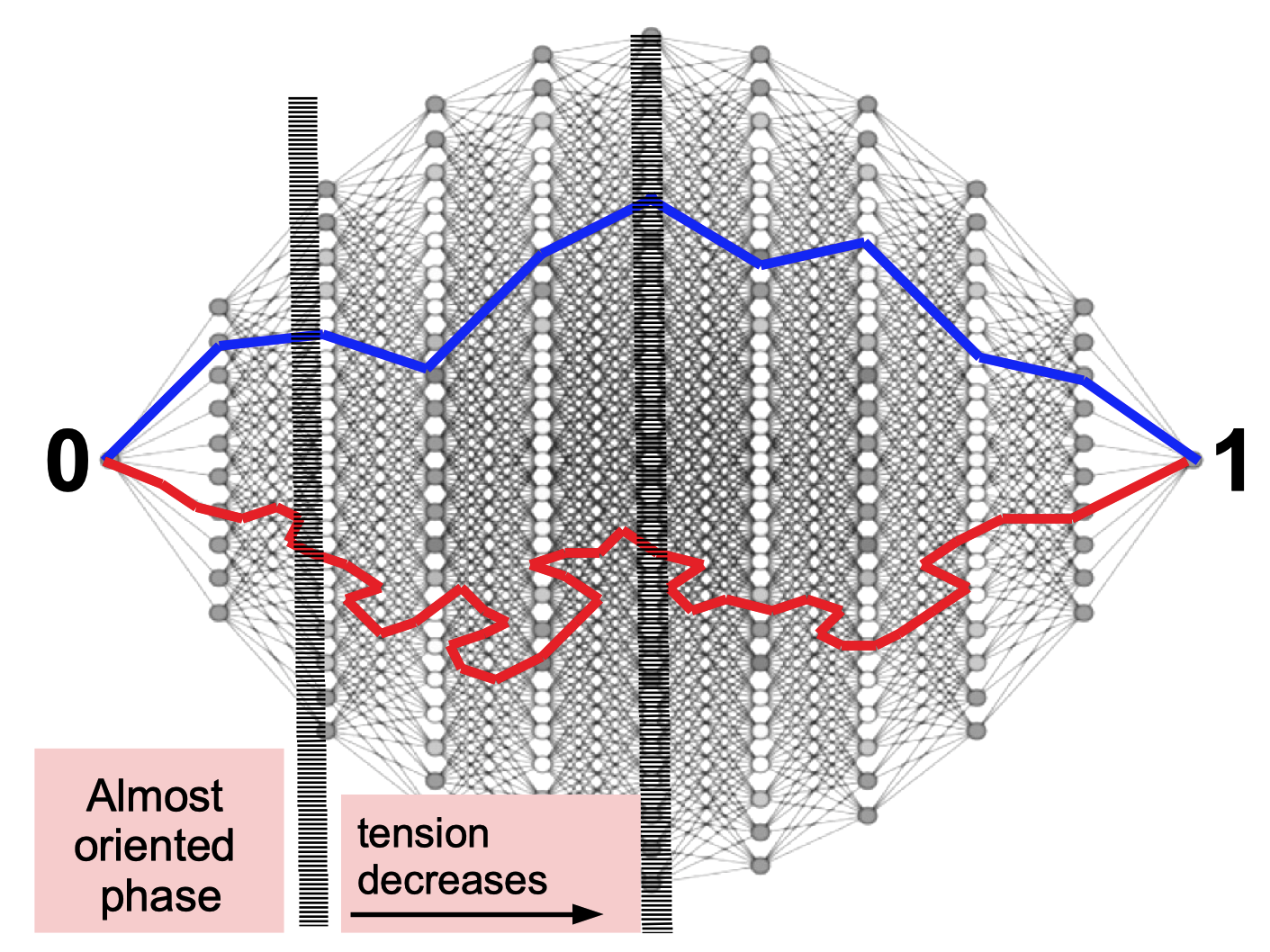
The two functions are plotted in Figure 4 below, whereas a rendition of the emerging picture at the level of the strands is given in Figure 5.

Refer to caption
Figure 4. Hamming-depth as a function of the length: directed (blue) vs. undirected (red) polymers. For small lengths, the depths are comparable: close to the origin, the undirected polymer is thus as directed as possible. The slope of the red curve decreases however gradually as the polymer approaches the core of the hypercube: the further the polymer goes, the ”loser” it becomes. Due to the inherent symmetry of the hypercube, a mirror picture sets in, of course, at half-length.
Refer to caption
Figure 5. Directed (blue) vs. undirected (red) polymers. The red strand starts off as stretched as possible, but allows for more and more backsteps as it approaches the core of the hypercube. The phenomena are amplified for better visualisation only: in line with Insight 4, backsteps live on meso/microscopic scale only. In particular, long excursions as in Figure 1 above are, in fact, ruled out.

2.4. Length vs. distance: the mesoscopic picture

As mentioned in the introduction, our approach will eventually rest on a multiscale analysis: in this section, inspired by the previous Insights, we introduce the necessary coarse graining [7]. To see how this goes, we denote by K∈ℕK\in\mathbb{N} the numbers of ”scales”, and shorten henceforth n^K≡n/K\hat{n}_{K}\equiv n/K (assuming w.l.o.g. that n^K∈ℕ\hat{n}_{K}\in\mathbb{N}). We then split the hypercube into KK ”slabs”, i.e. hyperplanes equidistributed w.r.t. the Hamming distance: for i=1​…​Ki=1\dots K we let

Hi≡{v∈Vn,d⁡(0,v)=i​n^K}.H_{i}\equiv\left\{v\in V_{n},d(0,v)=i\hat{n}_{K}\right\}\,. (2.24)

We will refer to these hyperplanes as HH-planes. Accordingly, we split a polymer of length 𝖫​n\mathsf{L}n into KK substrands of length αi​L​n\alpha_{i}Ln, for i=1​…​Ki=1\dots K, with the normalization ∑i≤Kαi=1\sum_{i\leq K}\alpha_{i}=1. We shorten 𝜶=(α1,α2,…,αK)∈[0,1]K\boldsymbol{\alpha}=(\alpha_{1},\alpha_{2},...,\alpha_{K})\in[0,1]^{K} for such a vector, 𝜶¯i≡∑j=1iαj\overline{\boldsymbol{\alpha}}_{i}\equiv\sum_{j=1}^{i}\alpha_{j} for the (fraction of) length of the strand when the polymer crosses the it​hi^{th} H-plane, and 𝜶¯i≡1−∑j=1iαj\underline{\boldsymbol{\alpha}}_{i}\equiv 1-\sum_{j=1}^{i}\alpha_{j} for the length of the remaining strand. A graphical rendition is given in Figure 6 below.

Refer to caption
Figure 6. KK-levels coarse graining: the Hamming distance between any two (successive) hyperplanes is n^K=n/K\hat{n}_{K}=n/K. Remark that by (2.26)-(2.27), the length of the substrand from hyperplane to hyperplane is a function of 𝖤\mathsf{E} and KK only.

By the above Insight 3, length of substrands and Hamming-depth must satisfy the fundamental relation

sinh⁡(𝜶¯i​𝖤)​cosh⁡(𝜶¯i​𝖤)=iK,i=1​…​K.\sinh(\overline{\boldsymbol{\alpha}}_{i}\mathsf{E})\cosh(\underline{\boldsymbol{\alpha}}_{i}\mathsf{E})=\frac{i}{K}\,,\quad i=1\dots K. (2.25)

The function x∈[0,1]↦sinh⁡(x​𝖤)​cosh⁡((1−x)​𝖤)x\in[0,1]\mapsto\sinh(x\mathsf{E})\cosh((1-x)\mathsf{E}) is invertible, and one can even construct explicitely the solutions of the above equation: recalling that arcsinh⁡(x)=log⁡(x+1+x2)\arcsinh(x)=\log(x+\sqrt{1+x^{2}}) one plainly checks that these are given by

𝜶¯i=12​{1+1𝖤​arcsinh⁡(2​iK−1)}.\overline{\boldsymbol{\alpha}}_{i}=\frac{1}{2}\left\{1+\frac{1}{\mathsf{E}}\arcsinh\left(2\frac{i}{K}-1\right)\right\}\,. (2.26)

This also uniquely identifies the length of the substrands, to wit:

αi=𝜶¯i−𝜶¯i−1,\alpha_{i}=\overline{\boldsymbol{\alpha}}_{i}-\overline{\boldsymbol{\alpha}}_{i-1}\,, (2.27)

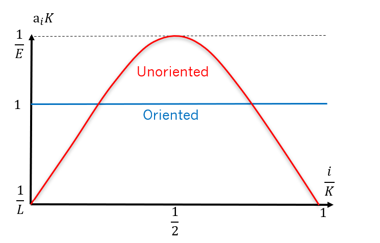
for i=1​…​Ki=1\dots K, see Figure 7 below for a plot.

In particular, it follows from (2.26) and (2.27) that

αi=αK+1−i,\alpha_{i}=\alpha_{K+1-i}, (2.28)

which is in full agreement with the inherent symmetry of the problem at hand, and ∑j≤Kαj=1\sum_{j\leq K}\alpha_{j}=1. Furthermore, since arcsinh\arcsinh is 11-Lipschitz we also immediately see that

αi≤1K​𝖤.\alpha_{i}\leq\frac{1}{K\mathsf{E}}. (2.29)

In order to emphasize that the α′​s\alpha^{\prime}s are no longer arbitrary, we will write henceforth 𝖺=𝖺⁡(𝖤,K)\mathsf{a}=\mathsf{a}(\mathsf{E},K) for the solutions of the equations (2.26), (2.27).
Refer to caption
Figure 7. Substrand-length as function of the depth, i∈{1,…​K}↦𝖺ii\in\{1,\dots K\}\mapsto\mathsf{a}_{i}. This plot simply restates the key property of optimal polymers: substrands between equidistant hyperplanes become longer as the polymer enters the core of the hypercube.

A straightforward large-KK Taylor expansion (with i/K=c​o​n​s​t.i/K=const.) yields that

𝖺i+1−𝖺i=2K2​𝖤​(1−2​iK)+O⁡(1K3),\mathsf{a}_{i+1}-\mathsf{a}_{i}=\frac{2}{K^{2}\mathsf{E}}\left(1-\frac{2i}{K}\right)+O\left(\frac{1}{K^{3}}\right)\,, (2.30)

which is manifestly different from the case of directed polymers, where the differential would necessarily vanish. Thus a fundamental question immediately arises:

how do substrands of undirected polymers connect
the coarse graining-hyperplanes?

To shed light on this issue we consider 𝒅=(d1,d2,…,dK)∈[0,1]K\boldsymbol{d}=(d_{1},d_{2},...,d_{K})\in[0,1]^{K} and introduce

Πi𝒅[𝒗→𝒘]≡\displaystyle\Pi_{i}^{\boldsymbol{d}}[\boldsymbol{v}\to\boldsymbol{w}]\equiv all loopless paths connecting\displaystyle\text{\sf all loopless paths connecting} (2.31)
two vertices​𝒗∈Hi−1,𝒘∈Hi\displaystyle\text{\sf two vertices}\;\boldsymbol{v}\in H_{i-1},\,\boldsymbol{w}\in H_{i}
which are at Hamming distance​d​(𝒗,𝒘)=di​n,\displaystyle\text{\sf which are at Hamming distance}\;d(\boldsymbol{v},\boldsymbol{w})=d_{i}n\,,

and

Π{1​…​K}𝒅[𝟎→𝟏]≡\displaystyle\Pi_{\{1\dots K\}}^{\boldsymbol{d}}[\boldsymbol{0}\to\boldsymbol{1}]\equiv all loopless paths connecting​ 0​to​ 1,\displaystyle\text{\sf all loopless paths connecting}\;\boldsymbol{0}\;\text{to}\;\boldsymbol{1}\;, (2.32)
and that cover a​di​n​-Hamming distance\displaystyle\text{\sf and that cover a}\;d_{i}n\text{\sf-Hamming distance}
while connecting the H-hyperplanes,​i=1​…​K.\displaystyle\text{\sf while connecting the H-hyperplanes,}\;i=1\dots K.

A graphical rendition is given in Figure 8 below.

Refer to caption
Figure 8. A polymer between two hyperplanes: the two vertices 𝒗\boldsymbol{v} and 𝒘\boldsymbol{w} are at a Hamming distance d⁡(𝒗,𝒘)=did(\boldsymbol{v},\boldsymbol{w})=d_{i}. Remark that, in particular, d⁡(Hi−1,Hi)=1/K≤di≤lπ​(𝒗,𝒘)d(H_{i-1},H_{i})=1/K\leq d_{i}\leq l_{\pi}(\boldsymbol{v},\boldsymbol{w}).

For π∈Π{1​…​K}𝒅[𝟎→𝟏]\pi\in\Pi_{\{1\dots K\}}^{\boldsymbol{d}}[\boldsymbol{0}\to\boldsymbol{1}], and two vertices 𝒗∈Hi−1,𝒘∈Hi\boldsymbol{v}\in H_{i-1},\boldsymbol{w}\in H_{i} (for some i=1​…​Ki=1\dots K), we furthermore shorten

Xπ​(𝒗,𝒘)≡\displaystyle X_{\pi}(\boldsymbol{v},\boldsymbol{w})\equiv energy of the substrand which connects​𝒗,𝒘.\displaystyle\text{energy of the substrand which connects}\;\boldsymbol{v},\,\boldsymbol{w}\,\,. (2.33)

and denote by

Ni𝒅[𝒗→𝒘]=#{π∈Πi𝒅[𝒗→𝒘],Xπ(𝒗,𝒘)≤𝖺i𝖤},N_{i}^{\boldsymbol{d}}[\boldsymbol{v}\to\boldsymbol{w}]=\#\left\{\pi\in\Pi_{i}^{\boldsymbol{d}}[\boldsymbol{v}\to\boldsymbol{w}],X_{\pi}(\boldsymbol{v},\boldsymbol{w})\leq\mathsf{a}_{i}\mathsf{E}\right\}\,, (2.34)

the number of substrands with energies at most 𝖺i​E\mathsf{a}_{i}E connecting such vertices. Finally, let

N{1​…​K}𝒅[𝟎→𝟏]=#{π∈Π{1​…​K}𝒅[𝟎→𝟏],Xπ(𝟎,𝟏)≤𝖤}N_{\{1\dots K\}}^{\boldsymbol{d}}[{\boldsymbol{0}\to\boldsymbol{1}}]=\#\left\{\pi\in\Pi_{\{1\dots K\}}^{\boldsymbol{d}}[\boldsymbol{0}\to\boldsymbol{1}],\ X_{\pi}(\boldsymbol{0},\boldsymbol{1})\leq\mathsf{E}\right\} (2.35)

stand for the number of paths with prescribed evolutions44 4 We shall perhaps emphasize that the above prescription of the evolution involves the Hamming-depths and energies, but not the length of the connecting substrands. This is because in (2.34) we are spreading the energies uniformly along the length of the polymer, very much in line with Insight 2: energies and optimal lengths are two sides of the same coin.. The goal is to compute the expectation of this random set, as this will provide fundamental insights into the possible choices of 𝒅\boldsymbol{d}, which are the only degrees of freedom left. As we will see shortly, there is only one reasonable choice. Before that we need however to introduce some key concepts.

Definition 2.1.

Let 𝐯∈Hi−1{\boldsymbol{v}}\in H_{i-1} and 𝐰∈Hi\boldsymbol{w}\in H_{i}.

  • •

    The effective forward steps are given by

    𝖾𝖿i​(𝒗,𝒘)≡1n​#​{0′​s​in​𝒗​which switch into​ 1′​s​in​𝒘}\mathsf{ef}_{i}(\boldsymbol{v},\boldsymbol{w})\equiv\frac{1}{n}\#\left\{0^{\prime}s\;\text{in}\;\boldsymbol{v}\;\text{which switch into}\;1^{\prime}s\;\text{in}\;\boldsymbol{w}\right\}
  • •

    The effective backsteps are given by

    𝖾𝖻i​(𝒗,𝒘)≡1n​#​{1′​s​in​𝒗​which switch into​ 0′​s​in​𝒘}.\mathsf{eb}_{i}(\boldsymbol{v},\boldsymbol{w})\equiv\frac{1}{n}\#\left\{1^{\prime}s\;\text{in}\;\boldsymbol{v}\;\text{which switch into}\;0^{\prime}s\;\text{in}\;\boldsymbol{w}\right\}\,.
  • •

    The detours are given by

    γπ​(𝒗,𝒘)≡1n​{lπ​(𝒗,𝒘)−d⁡(𝒗,𝒘)}.\gamma_{\pi}(\boldsymbol{v},\boldsymbol{w})\equiv\frac{1}{n}\left\{l_{\pi}(\boldsymbol{v},\boldsymbol{w})-d(\boldsymbol{v},\boldsymbol{w})\right\}.

Some comments concerning the above terminology are perhaps in place: we note that the effective forward steps encode the fraction of steps forward which are not undone by backsteps in the reverse direction; similarly, the effective backsteps encode the (fraction of) backsteps which are not undone by steps forward in the reverse direction (or vice versa). Finally, the detours capture the amount of forward steps in a path π\pi which are cancelled by backsteps in the reverse direction (or vice versa): the smaller γπ\gamma_{\pi}, the higher the ”tension” of the substrand. For this reason, we call a substrand stretched if the detours vanish. A stretched path is, in fact, a geodesic.

The above quantities are all intertwined. Indeed, it holds:

di=𝖾𝖿i​(𝒗,𝒘)+𝖾𝖻i​(𝒗,𝒘)and1K=𝖾𝖿i​(𝒗,𝒘)−𝖾𝖻i​(𝒗,𝒘).\displaystyle d_{i}=\mathsf{ef}_{i}(\boldsymbol{v},\boldsymbol{w})+\mathsf{eb}_{i}(\boldsymbol{v},\boldsymbol{w})\quad\text{and}\quad\frac{1}{K}=\mathsf{ef}_{i}(\boldsymbol{v},\boldsymbol{w})-\mathsf{eb}_{i}(\boldsymbol{v},\boldsymbol{w})\,. (2.36)

In particular, it follows from the above relations that

𝖾𝖿i​(𝒗,𝒘)=di2+12​Kand𝖾𝖻i​(𝒗,𝒘)=di2−12​K.\displaystyle\mathsf{ef}_{i}(\boldsymbol{v},\boldsymbol{w})=\frac{d_{i}}{2}+\frac{1}{2K}\quad\text{and}\quad\mathsf{eb}_{i}(\boldsymbol{v},\boldsymbol{w})=\frac{d_{i}}{2}-\frac{1}{2K}\,. (2.37)

In other words, effective forward- and backsteps along a substrand depend on the number of scales, and the remaining degrees of freedom 𝒅\boldsymbol{d} (which we are going to identify shortly), but not on the endpoints. An equally simple line of reasoning shows that detours, as soon as the polymer-length is specified, do not depend on the specific form of the π\pi-path, neither: in fact, γi,π​n+di​n=𝖺i​L​n\gamma_{i,\pi}n+d_{i}n=\mathsf{a}_{i}Ln.

As mentioned, the goal is to compute the expected number of paths connecting 𝟎\boldsymbol{0} to 𝟏\boldsymbol{1}. Since polymers are loopless, and by independence, it holds:

𝔼(N{1​…​K}𝒅[𝟎→𝟏])=∑(⋆)∏i=1K𝔼Ni𝒅[𝒗(i−1)→𝒗(i)],{\mathbb{E}}\left(N_{\{1\dots K\}}^{\boldsymbol{d}}[{\boldsymbol{0}\to\boldsymbol{1}}]\right)=\sum_{(\star)}\prod_{i=1}^{K}{\mathbb{E}}N_{i}^{\boldsymbol{d}}\left[\boldsymbol{v}^{(i-1)}\to\boldsymbol{v}^{(i)}\right], (2.38)

where the (⋆)(\star)-sum runs over all possible vertices 𝒗(i)∈Hi,i=1​…​K\boldsymbol{v}^{(i)}\in H_{i},i=1\dots K. But by (2.37), none of the expectations on the r.h.s. depend on the specific 𝒗\boldsymbol{v}-choice. The cardinality of (⋆)(\star) is easily computed: shortening

[0,∞)∋x↦φ⁡(x)≡xx,[0,\infty)\ni x\mapsto\varphi(x)\equiv x^{x}, (2.39)

one plainly checks that

#⁡(⋆)\displaystyle\#(\star) =∏i=1K(i−1K​n𝖾𝖻i​n)​((1−i−1K)​n𝖾𝖿i​n)\displaystyle=\prod_{i=1}^{K}\dbinom{\frac{i-1}{K}n}{\mathsf{eb}_{i}n}\dbinom{\left(1-\frac{i-1}{K}\right)n}{\mathsf{ef}_{i}n} (2.40)
≲∏i=1K{φ⁡(i−1K)​φ​(1−i−1K)φ⁡(𝖾𝖻i)​φ​(i−1K−𝖾𝖻i)​φ​(𝖾𝖿i)​φ​(1−i−1K−𝖾𝖿i)}n,\displaystyle\lesssim\prod_{i=1}^{K}\left\{\frac{\varphi\left(\frac{i-1}{K}\right)\varphi\left(1-\frac{i-1}{K}\right)}{\varphi(\mathsf{eb}_{i})\varphi\left(\frac{i-1}{K}-\mathsf{eb}_{i}\right)\varphi\left(\mathsf{ef}_{i}\right)\varphi\left(1-\frac{i-1}{K}-\mathsf{ef}_{i}\right)}\right\}^{n}\,,

the last step by elementary Stirling-approximation to first order.

By the tail estimates, and Stanley’s M-bound (2.14) with x=𝖺i​𝖤x=\mathsf{a}_{i}\mathsf{E} , it holds

𝔼Ni𝒅[𝒗(i−1)→𝒗(i)]≲sinh(𝖺i𝖤)di​ncosh(𝖺i𝖤)(1−di)​n,\displaystyle{\mathbb{E}}N_{i}^{\boldsymbol{d}}\left[\boldsymbol{v}^{(i-1)}\to\boldsymbol{v}^{(i)}\right]\lesssim{\sinh(\mathsf{a}_{i}\mathsf{E})}^{d_{i}n}{\cosh(\mathsf{a}_{i}\mathsf{E})}^{(1-d_{i})n}\,, (2.41)

for i=1​…​Ki=1\dots K.

Plugging (2.40) and (2.41) into (2.38), and rearranging, we thus get the upperbound

𝔼(N{1​…​K}𝒅[𝟎→𝟏])\displaystyle{\mathbb{E}}\left(N_{\{1\dots K\}}^{\boldsymbol{d}}[{\boldsymbol{0}\to\boldsymbol{1}}]\right) ≲ℱ𝖺,K​(𝒅)n,\displaystyle\lesssim\mathcal{F}_{\mathsf{a},K}(\boldsymbol{d})^{n}, (2.42)

where we have shortened

ℱ𝗮,K​(𝒅)≡∏i=1Ksinh(𝖺iE)dicosh(𝖺iE)(1−di)φ(i−1K)φ(1−i−1K)φ⁡(𝖾𝖻i)​φ​(i−1K−𝖾𝖻i)​φ​(𝖾𝖿i)​φ​(1−i−1K−𝖾𝖿i).\mathcal{F}_{\boldsymbol{\mathsf{a}},K}(\boldsymbol{d})\equiv\prod_{i=1}^{K}\frac{{\sinh(\mathsf{a}_{i}E)}^{d_{i}}{\cosh(\mathsf{a}_{i}E)}^{(1-d_{i})}\varphi\left(\frac{i-1}{K}\right)\varphi\left(1-\frac{i-1}{K}\right)}{\varphi(\mathsf{eb}_{i})\varphi\left(\frac{i-1}{K}-\mathsf{eb}_{i}\right)\varphi\left(\mathsf{ef}_{i}\right)\varphi\left(1-\frac{i-1}{K}-\mathsf{ef}_{i}\right)}\,. (2.43)

Since 𝗮=𝗮⁡(𝖤,K)\boldsymbol{\mathsf{a}}=\boldsymbol{\mathsf{a}}(\mathsf{E},K) are solutions of (2.26)-(2.27), the 𝒅′​s\boldsymbol{d}^{\prime}s appearing in the ℱ\mathcal{F}-function are the only degrees of freedom left (By (2.37), we recall that 𝖾𝖿i\mathsf{ef}_{i} and 𝖾𝖻i\mathsf{eb}_{i} are function of did_{i}). The next result shows that even for these, there is in fact one reasonable choice only.

Theorem 1.

(Optimal Hamming distance) Let 𝗱=(𝖽1,…,𝖽K)\boldsymbol{\mathsf{d}}=(\mathsf{d}_{1},\dots,\mathsf{d}_{K}), with

𝖽i≡sinh⁡(𝖺i​𝖤)​cosh⁡((1−𝖺i)​𝖤).\mathsf{d}_{i}\equiv\sinh(\mathsf{a}_{i}\mathsf{E})\cosh((1-\mathsf{a}_{i})\mathsf{E}). (2.44)

It then holds:

ℱ𝗮,K​(𝗱)=1,\mathcal{F}_{\boldsymbol{\mathsf{a}},K}(\boldsymbol{\mathsf{d}})=1, (2.45)

and

ℱ𝗮,K​(𝒅)<1,for𝒅≠𝗱.\mathcal{F}_{\boldsymbol{\mathsf{a}},K}(\boldsymbol{d})<1,\quad\text{for}\quad\boldsymbol{d}\neq\boldsymbol{\mathsf{d}}. (2.46)

By (2.42) and (2.46), the expected number of polymers connecting a sequence of prescribed vertices on the HH-planes is thus exponentially small, unless the Hamming distance of the considered vertices satisfies (2.44): of course, the latter will henceforth be the value of our choice.

Theorem 1 is absolutely crucial for our approach. The proof, which requires a fair amount of work, is postponed. For the remaining part of this section we dwell rather informally on some of its far-reaching implications.

We anticipate that we will eventually consider a large (yet finite) number of scales for the coarse graining, in which case an elementary large-KK Taylor expansion (together with the fact that 𝖫=2​𝖤\mathsf{L}=\sqrt{2}\mathsf{E}) shows that to first approximation, Hamming distance between two vertices on the H-planes and substrand-legth do, in fact, coincide:

𝖽i=\displaystyle\mathsf{d}_{i}= sinh⁡(𝖺i​𝖤)​cosh⁡((1−𝖺i)​𝖤)=𝖺i​𝖫+O⁡(1K2).\displaystyle\sinh(\mathsf{a}_{i}\mathsf{E})\cosh((1-\mathsf{a}_{i})\mathsf{E})=\mathsf{a}_{i}\mathsf{L}+O\left(\frac{1}{K^{2}}\right)\,. (2.47)

A minute’s thought suggests that the above may be reformulated as follows:

Insight 5.
Optimal polymers connect the coarse graining H-planes through essentially stretched paths.

This is a somewhat surprising feature, which at first sight may even appear non-sensical. The devil is however in the details: by (2.26), and large-KK Taylor expansions (again with i/K=c​o​n​s​ti/K=const), one can check that

𝖺i=1K​𝖤​1+(2​iK−1)2+O⁡(1K2),\mathsf{a}_{i}=\frac{1}{K\mathsf{E}\sqrt{1+(\frac{2i}{K}-1)^{2}}}+O\left(\frac{1}{K^{2}}\right)\,, (2.48)

which combined with (2.47), and recalling 𝖫=2​𝖤\mathsf{L}=\sqrt{2}\mathsf{E}, leads to

𝖽i=2K​1+(2​iK−1)2+O⁡(1K2).\mathsf{d}_{i}=\frac{\sqrt{2}}{K\sqrt{1+\left(\frac{2i}{K}-1\right)^{2}}}+O\left(\frac{1}{K^{2}}\right)\,. (2.49)

From this we may evince that:

  • •

    for small ii (say i=s​Ki=sK, and s≪1/2s\ll 1/2) it holds that

    𝖺i=1K​𝖤​2+O⁡(1K2)=1K​𝖫+O⁡(1K2),\mathsf{a}_{i}=\frac{1}{K\mathsf{E}\sqrt{2}}+O\left(\frac{1}{K^{2}}\right)=\frac{1}{K\mathsf{L}}+O\left(\frac{1}{K^{2}}\right)\,, (2.50)

    as well as

    𝖽i=1K+O⁡(1K2)=d⁡(Hi−1,Hi)+O⁡(1K2),\mathsf{d}_{i}=\frac{1}{K}+O\left(\frac{1}{K^{2}}\right)=d(H_{i-1},H_{i})+O\left(\frac{1}{K^{2}}\right)\,, (2.51)

    the latter confirming that close to the origin, unoriented polymers proceed in almost directed fashion;

  • •

    for large ii (say i=s​Ki=sK, and s↑1/2s\uparrow 1/2) it holds that 𝖽i≈2/K≫1/K\mathsf{d}_{i}\approx\sqrt{2}/K\gg 1/K, which is much larger than the Hamming distance between two successive H-planes. Substrands of optimal polymers close to the core of the hypercube therefore reach, through approximate geodesics, vertices which are otherwise unattainable in a fully directed regime. Although the length of the substrand is increased, this strategy allows undirected polymers to gain access to a reservoir of energetically favorable edges. A graphical rendition of this feature, which encodes the key strategy of optimal polymers, is given in Figure 9 below.

Refer to caption
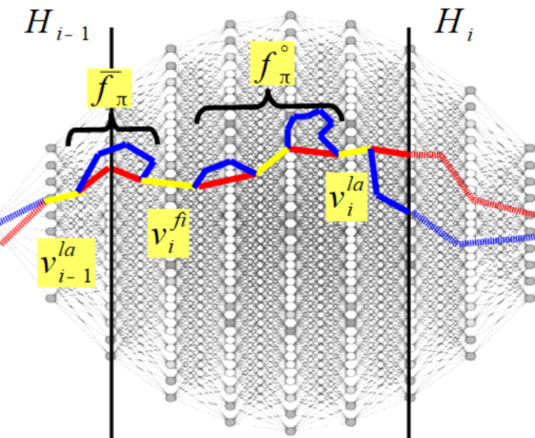
Figure 9. The black-shaded cone corresponds to the region where a fully directed polymer would lie. In virtue of Theorem 1, the optimal, undirected polymers evolve however in the red-shaded cones, thereby reaching vertices which are at larger Hamming distance. (Note also that black and red vertical boundaries of these cones are disjunct). For large hyperplane-density, the substrands (in red) of optimal polymers are, in first approximation, geodesics.

The feature according to which undirected polymers proceed through approximate geodesics is absolutely fundamental. On the one hand it neatly explains the deeper mechanisms eventually responsible for the onset of the mean field trivialization. On a more technical level, this property will lead to a dramatic simplification of some otherwise daunting combinatorial estimates, eventually enabling us to implement the second moment method. In fact, in a (fully) stretched regime, a backstep cannot be cancelled by a forward step (and vice versa). This entails, in particular, a natural representation of paths connecting say 𝒗∈Hi−1\boldsymbol{v}\in H_{i-1} to 𝒘∈Hi\boldsymbol{w}\in H_{i} in terms of permutations of the 𝒗\boldsymbol{v}-coordinates which must be changed in order to obtain 𝒘\boldsymbol{w}, see in particular Lemma 21 below for a clear manifestation of this feature.

2.5. Main result

We now specify a subset of polymers with path properties capturing all Insights gathered so far: our main result, which is at last formulated in this section, simply states that such a subset is, in fact, non-empty. Towards this goal, some additional observations/notation is needed.

For arbitrary 𝒅=(d1,…,dK)∈[0,1)K\boldsymbol{d}=(d_{1},\dots,d_{K})\in[0,1)^{K} (the Hamming-depths) and 𝜸=(γ1,…,γK)∈[0,∞)K\boldsymbol{\gamma}=(\gamma_{1},\dots,\gamma_{K})\in[0,\infty)^{K} (the detours), consider the subset

𝒫n,K​{𝒅,𝜸}≡\displaystyle\mathcal{P}_{n,K}\left\{\boldsymbol{d},\boldsymbol{\gamma}\right\}\equiv all paths connecting​ 0​to​ 1,\displaystyle\text{\sf all paths connecting}\;\boldsymbol{0}\;\text{to}\;\boldsymbol{1}\;, (2.52)
and that cover a normalized​di​-Hamming distance,\displaystyle\text{\sf and that cover a normalized}\;d_{i}\text{\sf-Hamming distance},
with​γi​detours,\displaystyle\text{\sf with}\;\gamma_{i}\;\text{\sf detours},
while connecting the H-hyperplanes,​i=1​…​K.\displaystyle\text{\sf while connecting the H-hyperplanes,}\;i=1\dots K\,.

We now make a specific choice of the free parameters, 𝒅\boldsymbol{d} and 𝜸\boldsymbol{\gamma}, which is naturally justified by the picture canvassed in the above sections. As a matter of fact, we will force polymers to reflect an ”extreme” version of the picture. Precisely:

  • •

    instead of considering polymers which are essentially directed close to the endpoints (recall in particular Figure 4) we will consider polymers which are fully directed in these regimes. We will achieve this by fixing a small m=205≪Km=205\ll K (as already mentioned, we will choose KK large enough). With 𝗱=(𝖽1,…,𝖽K)\boldsymbol{\mathsf{d}}=(\mathsf{d}_{1},\dots,\mathsf{d}_{K}) the optimal Hamming distance as in (2.44) from Theorem 1 we then set

    𝗱o​p​t=(1/K,…,1/K⏟m−times,𝖽m+1,𝖽m+2,…,𝖽K−m,1/K,…,1/K⏟m−times),\displaystyle\boldsymbol{\mathsf{d}}_{opt}=\left(\underbrace{1/K,\dots,1/K}_{m-\text{times}},\mathsf{d}_{m+1},\mathsf{d}_{m+2},...,\mathsf{d}_{K-m},\underbrace{1/K,\dots,1/K}_{m-\text{times}}\right)\,, (2.53)
  • •

    instead of considering polymers which are essentially stretched between the coarse graining H-planes (recall in particular Insight 5), we will consider polymers which proceed through exact geodesics; this will be achieved by setting

    𝜸o​p​t≡(0,…,0).{\boldsymbol{\gamma}}_{opt}\equiv(0,\dots,0)\,. (2.54)

Denoting by 𝖫o​p​t\mathsf{L}_{opt} the normalized length of paths in 𝒫n,K​{𝗱o​p​t,𝜸o​p​t}\mathcal{P}_{n,K}\left\{\boldsymbol{\mathsf{d}}_{opt},{\boldsymbol{\gamma}}_{opt}\right\}, it holds that

𝖫o​p​t=‖𝗱o​p​t‖1.\mathsf{L}_{opt}=\|\boldsymbol{\mathsf{d}}_{opt}\|_{1}\,. (2.55)

We then focus on the ensuing subset 𝒫n,K​{𝗱o​p​t,𝜸o​p​t}⊂Π~n,𝖫o​p​t​n\mathcal{P}_{n,K}\left\{\boldsymbol{\mathsf{d}}_{opt},{\boldsymbol{\gamma}}_{opt}\right\}\subset\widetilde{\Pi}_{n,\mathsf{L}_{opt}n}. A graphical rendition of these polymers, which are only marginally shorter than 𝖫=2​𝖤\mathsf{L}=\sqrt{2}\mathsf{E} (see (2.59) below for more on this), is given in Figure 10.

Refer to caption
Figure 10. A polymer in 𝒫n,K\mathcal{P}_{n,K}: the blue substrand is fully directed. The red substrands connect the H-planes of the coarse graining through stretched paths, i.e. geodesics.

Since Hamming-depths and detours are specified, we lighten henceforth notation by

𝒫n,K≡𝒫n,K​{𝗱o​p​t,𝜸o​p​t}.\mathcal{P}_{n,K}\equiv\mathcal{P}_{n,K}\left\{\boldsymbol{\mathsf{d}}_{opt},{\boldsymbol{\gamma}}_{opt}\right\}. (2.56)

Let now ϵ>0\epsilon>0, and consider the subset of polymers

ℰn,Kϵ≡π∈𝒫n,K​with energies​Xπ≤𝖤+ϵ,\mathcal{E}_{n,K}^{\epsilon}\equiv\pi\in\mathcal{P}_{n,K}\;\text{\sf with energies}\;X_{\pi}\leq\mathsf{E}+\epsilon\,, (2.57)

namely those paths which i) are fully directed close to the endpoints, ii) connect the coarse graining H-planes in the core of the hypercube through geodesics, iii) and which reach an ϵ\epsilon-neighborhood of the ground state energy. Our main result states that such polymers do, in fact, exist:

Theorem 2.

(The geometry of optimal polymers). For ϵ>0\epsilon>0 there exists K=K⁡(ϵ)∈ℕK=K(\epsilon)\in\mathbb{N} such that

limn→∞ℙ⁡(#​ℰn,Kϵ≥1)=1.\lim_{n\to\infty}{\mathbb{P}\left(\#\,\mathcal{E}_{n,K}^{\epsilon}\geq 1\right)}=1. (2.58)

The proof of Theorem 2, which eventually boils down to an application of the Paley-Zygmund inequality, is both technically demanding and long, and will be given in the next sections. Before seeing how this goes, some comments are in order.

First, we remark that the length of the substrands connecting the H-planes (which is related to the 𝖺′​s\mathsf{a}^{\prime}s) does not appear explicitely in the statement of Theorem 2, and neither do the sub-energies. This is again due to the fact that, in line with Insight 2, uniformly spread lengths/energies will be hiding behind the optimal Hamming-depths.

Second, we point out that Theorem 2, when combined with the simple lower bound discussed in the Introduction, yields a constructive proof of Martinsson’s Theorem.

Lastly, and with the unsettled issue of fluctuations in mind, we shall dwell on a conceptually intricate aspect of the theorem, namely the nature of the parameter KK encoding the density of hyperplanes for the coarse graining. One perhaps expects that larger constants lead to more accurate pictures, but this is only to some extent correct. In fact, too large hyperplane-density would even lead to inconsistencies: higher and higher densities ”unbend” the strands, ultimately to the point of complete directedness, but this, in turn, would starkly contradict the crucial feature of optimal polymers, namely that their length is larger than the dimension. A delicate balance must therefore be met. As we will see in the course of the second moment implementation, see (6.52), (6.82), (6.87) and (6.134) below, for the present purpose of analyzing the ground state to leading order, it indeed suffices to take a large but finite K=max⁡{2×10⁷,m​ϵ−2}K=\max\left\{2\times 10^{7},m\epsilon^{-2}\right\}. How fast (in the dimension nn) the hyperplane-density can be allowed to grow is an interesting, and important issue, which unfortunately eludes us.

We conclude this section with the aforementioned result concerning the concentration of the length of optimal polymers, as this provides a neat round-off of the picture. To this end, remark that Theorem 2 involves paths of length 𝖫o​p​t\mathsf{L}_{opt}; by a more detailed study of taylor’s remainder term in (2.47), (2.50) and (2.51), and recalling that 𝖫=2​𝖤\mathsf{L}=\sqrt{2}\mathsf{E}, it can be plainly checked that

0≤𝖫−𝖫o​p​t≤mK.0\leq\mathsf{L}-\mathsf{L}_{opt}\leq\frac{m}{K}\,. (2.59)

In other words, for large hyperplane density, the difference between 𝖫o​p​t\mathsf{L}_{opt} and 𝖫\mathsf{L} is vanishing. Our second main result states that the length 𝖫\mathsf{L} is, in fact, optimal:

Theorem 3.

(Concentration of the polymer’s length). For ϵ>0\epsilon>0 and a>𝖤2+2​𝖤+12a>\frac{\mathsf{E}}{2}+\sqrt{2}\mathsf{E}+\frac{1}{\sqrt{2}},

limn→∞ℙ(#{π∈Πn:Xπ≤𝖤+ϵ2,1n|lπ(𝟎,𝟏)−𝖫n|≥aϵ}≥1)=0.\displaystyle\lim_{n\to\infty}\mathbb{P}\left(\#\left\{\pi\in\Pi_{n}:\;X_{\pi}\leq\mathsf{E}+\epsilon^{2},\frac{1}{n}|l_{\pi}(\boldsymbol{0},\boldsymbol{1})-\mathsf{L}n|\geq a\epsilon\right\}\geq 1\right)=0\,. (2.60)
Remark 6.

The proof of the above Theorem, which is given in Section 8 below, suggests (albeit feebly) that the (ϵ2,ϵ)(\epsilon^{2},\epsilon)-scaling in (2.60) is, in fact, optimal, and this in turn suggests that a central limit theorem applies for the optimal length.

The rest of the paper is organised as follows. In the next Section 3 we will provide a proof of Theorem 1. In Section 4, and for technical reasons which will become clear in the course of the treatment, some additional restrictions on the candidate optimal polymers will be specified: this will lead to the identification of a subset of 𝒫n,K\mathcal{P}_{n,K} on which we will henceforth focus our attention. Specifying these additional requirements will have an impact on the first moment as controlled in Theorem 1, and these modifications will be dealt with in Section 5. Section 6 forms the main body of the paper: there we will set up the second moment approach, postponing, however, the highly technical issues concerning the required path-counting to Section 7. Finally, the proof of optimality of the length 𝖫\mathsf{L} is given in Section 8.

3. The optimal Hamming distance: proof of Theorem 1

Recall that φ⁡(x)=xx\varphi(x)=x^{x} for x≥0x\geq 0, with the convention 00=10^{0}=1. We shorten

gj,K​(x)≡sinh(𝖺j𝖤)xcosh(𝖺j𝖤)(1−x)φ(j−1K)φ(1−j−1K)φ⁡(x2−12​K)​φ​(j−1K−(x2−12​K))​φ​(x2+12​K)​φ​(1−j−1K−(x2+12​K)),\displaystyle g_{j,K}(x)\equiv\frac{{\sinh(\mathsf{a}_{j}\mathsf{E})}^{x}{\cosh(\mathsf{a}_{j}\mathsf{E})}^{(1-x)}\varphi\left(\frac{j-1}{K}\right)\varphi\left(1-\frac{j-1}{K}\right)}{\varphi\left(\frac{x}{2}-\frac{1}{2K}\right)\varphi\left(\frac{j-1}{K}-(\frac{x}{2}-\frac{1}{2K})\right)\varphi\left(\frac{x}{2}+\frac{1}{2K}\right)\varphi\left(1-\frac{j-1}{K}-(\frac{x}{2}+\frac{1}{2K})\right)}\,, (3.1)

in which case, in virtue of (2.37), we may represent the ℱ\mathcal{F}-function as

ℱ𝗮,K​(𝒅)=∏j=1Kgj,K​(dj).\displaystyle\mathcal{F}_{\boldsymbol{\mathsf{a}},K}(\boldsymbol{d})=\prod_{j=1}^{K}g_{j,K}(d_{j})\,. (3.2)

Since the terms in the product on the r.h.s. are non-interacting, we clearly have

max𝒅⁡{ℱ𝗮,K​(𝒅)}=∏j=1Kmaxx≥0⁡{gj,K​(x)}.\displaystyle\max_{\boldsymbol{d}}\{\mathcal{F}_{\boldsymbol{\mathsf{a}},K}(\boldsymbol{d})\}=\prod_{j=1}^{K}\max_{x\geq 0}\{g_{j,K}(x)\}. (3.3)

We now claim that

∏j=1Kmaxx≥0⁡{gj,K​(x)}=1,\displaystyle\prod_{j=1}^{K}\max_{x\geq 0}\{g_{j,K}(x)\}=1, (3.4)

and

arg⁡maxx≥0​{gj,K​(x)}=𝖽j,\displaystyle\arg\max_{x\geq 0}\ \{g_{j,K}(x)\}=\mathsf{d}_{j}, (3.5)

with 𝖽j\mathsf{d}_{j} as in (2.44).

We will prove (3.5) first. We begin with the cases j=1,Kj=1,K and claim that

arg⁡maxx≥0​g1,K​(x)=arg⁡maxx≥0​gK,K​(x)=1K,\arg\max_{x\geq 0}g_{1,K}(x)=\arg\max_{x\geq 0}g_{K,K}(x)=\frac{1}{K}\,, (3.6)

and

1K=𝖽1=𝖽K.\frac{1}{K}=\mathsf{d}_{1}=\mathsf{d}_{K}. (3.7)

In fact, g1,K​(x)g_{1,K}(x) involves the terms

φ⁡(x2−12​K),\displaystyle\varphi\left(\frac{x}{2}-\frac{1}{2K}\right), (3.8)
φ⁡(j−1K−{x2−12​K})|j=1\displaystyle\varphi\left(\frac{j-1}{K}-\left\{\frac{x}{2}-\frac{1}{2K}\right\}\right)\Big|_{j=1} =φ⁡(12​K−x2),\displaystyle=\varphi\left(\frac{1}{2K}-\frac{x}{2}\right),

but for both to be properly defined it must hold

x2−12​K≥0,and12​K−x2≥0,\frac{x}{2}-\frac{1}{2K}\geq 0,\quad\text{and}\quad\frac{1}{2K}-\frac{x}{2}\geq 0, (3.9)

implying x=1Kx=\frac{1}{K}. A similar reasoning applies to gK,Kg_{K,K}, and (3.6) is settled. Claim (3.7) follows from (2.25) for the j=1j=1 case, whereas the j=Kj=K case follows by symmetry, see in particular (2.28).

Concerning the other indices, we fix j∈{2,…,K−1}j\in\{2,\dots,K-1\} and shorten, for x≥0x\geq 0,

gj,K​(x)≡Nj,K​(x)Dj,K​(x),\displaystyle g_{j,K}(x)\equiv\frac{N_{j,K}(x)}{D_{j,K}(x)}, (3.10)

where

Nj,K(x)≡sinh(𝖺j𝖤)xcosh(𝖺j𝖤)(1−x)φ(j−1K)φ(1−j−1K),\displaystyle N_{j,K}(x)\equiv{\sinh(\mathsf{a}_{j}\mathsf{E})}^{x}{\cosh(\mathsf{a}_{j}\mathsf{E})}^{(1-x)}\varphi\left(\frac{j-1}{K}\right)\varphi\left(1-\frac{j-1}{K}\right), (3.11)

and

Dj,K​(x)≡φ⁡(x2−12​K)​φ​(jK−x2−12​K)​φ​(x2+12​K)​φ​(1−jK−x2+12​K).\displaystyle D_{j,K}(x)\equiv\varphi\left(\frac{x}{2}-\frac{1}{2K}\right)\varphi\left(\frac{j}{K}-\frac{x}{2}-\frac{1}{2K}\right)\varphi\left(\frac{x}{2}+\frac{1}{2K}\right)\varphi\left(1-\frac{j}{K}-\frac{x}{2}+\frac{1}{2K}\right). (3.12)

Taking the xx-derivative, we see that

gj,K​(x)′>0⇔Nj,K​(x)′​Dj,K​(x)>Nj,K​(x)​Dj,K​(x)′.\displaystyle g_{j,K}(x)^{\prime}>0\iff{N_{j,K}(x)}^{\prime}D_{j,K}(x)>N_{j,K}(x){D_{j,K}(x)}^{\prime}. (3.13)

An elementary computation then yields

Nj,K​(x)′=Nj,K​(x)​log⁡(tanh⁡(𝖺j​𝖤)),\displaystyle{N_{j,K}(x)}^{\prime}=N_{j,K}(x)\log(\tanh(\mathsf{a}_{j}\mathsf{E})), (3.14)

and

Dj,K​(x)′=12​Dj,K​(x)​log⁡{(x2−12​K)​(x2+12​K)(jK−x2−12​K)​(1−jK−x2+12​K)}.\displaystyle{D_{j,K}(x)}^{\prime}=\frac{1}{2}D_{j,K}(x)\log\left\{\frac{(\frac{x}{2}-\frac{1}{2K})(\frac{x}{2}+\frac{1}{2K})}{(\frac{j}{K}-\frac{x}{2}-\frac{1}{2K})(1-\frac{j}{K}-\frac{x}{2}+\frac{1}{2K})}\right\}. (3.15)

Combining (3.13), (3.14) and (3.15), we therefore get

gi,K​(x)′>0⇔tanh⁡(𝖺j​𝖤)2>(x2−12​K)​(x2+12​K)(jK−x2−12​K)​(1−jK−x2+12​K).\displaystyle g_{i,K}(x)^{\prime}>0\iff{\tanh(\mathsf{a}_{j}\mathsf{E})}^{2}>\frac{(\frac{x}{2}-\frac{1}{2K})(\frac{x}{2}+\frac{1}{2K})}{(\frac{j}{K}-\frac{x}{2}-\frac{1}{2K})(1-\frac{j}{K}-\frac{x}{2}+\frac{1}{2K})}. (3.16)

Consider now

tanh⁡(𝖺j​𝖤)2=(x2−12​K)​(x2+12​K)(jK−x2−12​K)​(1−jK−x2+12​K).\displaystyle{\tanh(\mathsf{a}_{j}\mathsf{E})}^{2}=\frac{(\frac{x}{2}-\frac{1}{2K})(\frac{x}{2}+\frac{1}{2K})}{\left(\frac{j}{K}-\frac{x}{2}-\frac{1}{2K}\right)(1-\frac{j}{K}-\frac{x}{2}+\frac{1}{2K})}. (3.17)

This is a quadratic equation (in xx), whose unique positive solution is given by

x^≡−sinh⁡(𝖺j​𝖤)2+sinh(𝖺j𝖤)4+4sinh(𝖺j𝖤)2{2​j−12​K−j⁡(j−1)K2}+1K2.\displaystyle\hat{x}\equiv-{\sinh(\mathsf{a}_{j}\mathsf{E})}^{2}+\sqrt{{\sinh(\mathsf{a}_{j}\mathsf{E})}^{4}+4{\sinh(\mathsf{a}_{j}\mathsf{E})}^{2}\left\{\frac{2j-1}{2K}-\frac{j(j-1)}{K^{2}}\right\}+\frac{1}{K^{2}}}. (3.18)

A straightforward analysis shows that the quotient on the r.h.s. of (3.16) is, in fact, increasing in xx: in other words, the xx-derivative gi,K′g_{i,K}^{\prime} is positive for x<x^x<\hat{x} and negative for x>x^x>\hat{x}, implying that x^\hat{x} is indeed the extremal point. To finish the proof of (3.5) it thus remains to show that x^=𝖽j\hat{x}=\mathsf{d}_{j}, i.e. that x^=sinh⁡(𝖺j​𝖤)​cosh⁡((1−𝖺j)​𝖤)\hat{x}=\sinh(\mathsf{a}_{j}\mathsf{E})\cosh((1-\mathsf{a}_{j})\mathsf{E}). In order to do so, we will avoid the use of the explicit formulation (3.18), but rely rather on the expression (3.17) and the following

Lemma 7.

Let d∈ℝd\in\mathbb{R} satisfy

d2−12​K=sinh⁡(𝖺¯j−1​𝖤)​sinh⁡(𝖺j​𝖤)​sinh⁡(𝖺¯j​𝖤).\frac{d}{2}-\frac{1}{2K}=\sinh(\overline{\mathsf{a}}_{j-1}\mathsf{E})\sinh(\mathsf{a}_{j}\mathsf{E})\sinh(\underline{\mathsf{a}}_{j}\mathsf{E})\,. (3.19)

Then the above, and the following relations are all equivalent:

1−jK−d2+12​K=cosh⁡(𝖺¯j−1​𝖤)​cosh⁡(𝖺j​𝖤)​sinh⁡(𝖺¯j​𝖤),1-\frac{j}{K}-\frac{d}{2}+\frac{1}{2K}=\cosh(\overline{\mathsf{a}}_{j-1}\mathsf{E})\cosh(\mathsf{a}_{j}\mathsf{E})\sinh(\underline{\mathsf{a}}_{j}\mathsf{E}), (3.20)
\displaystyle d2+12​K=cosh⁡(𝖺¯j−1​𝖤)​sinh⁡(𝖺j​𝖤)​cosh⁡(𝖺¯j​𝖤),\displaystyle\frac{d}{2}+\frac{1}{2K}=\cosh(\overline{\mathsf{a}}_{j-1}\mathsf{E})\sinh(\mathsf{a}_{j}\mathsf{E})\cosh(\underline{\mathsf{a}}_{j}\mathsf{E}), (3.21)
jK−d2−12​K=sinh⁡(𝖺¯j−1​𝖤)​cosh⁡(𝖺j​𝖤)​cosh⁡(𝖺¯j​𝖤).\frac{j}{K}-\frac{d}{2}-\frac{1}{2K}=\sinh(\overline{\mathsf{a}}_{j-1}\mathsf{E})\cosh(\mathsf{a}_{j}\mathsf{E})\cosh(\underline{\mathsf{a}}_{j}\mathsf{E}). (3.22)

It follows in particular, that for such dd it holds d=x^d=\hat{x}, and d=𝖽jd=\mathsf{d}_{j}.

Proof of Lemma 7.

We first prove the equivalence of

(3.19)⇔(3.20)⇔(3.21)⇔(3.22),\displaystyle\eqref{e_1}\iff\eqref{e_3}\iff\eqref{e_2}\iff\eqref{e_4}, (3.23)

Indeed, by (2.25) and the fact that

sinh⁡(𝖺j¯​𝖤)​cosh⁡(𝖺¯j​𝖤)+cosh⁡(𝖺¯j​𝖤)​sinh⁡(𝖺¯j​𝖤)=1,\displaystyle\sinh(\overline{\mathsf{a}_{j}}\mathsf{E})\cosh(\underline{\mathsf{a}}_{j}\mathsf{E})+\cosh(\overline{\mathsf{a}}_{j}\mathsf{E})\sinh(\underline{\mathsf{a}}_{j}\mathsf{E})=1, (3.24)

it holds:

sinh⁡(𝖺¯j​𝖤)​cosh⁡(𝖺¯j​𝖤)=1−jK\sinh(\underline{\mathsf{a}}_{j}\mathsf{E})\cosh(\overline{\mathsf{a}}_{j}\mathsf{E})=1-\frac{j}{K} (3.25)

for all j=1​…​Kj=1\dots K. Relation (3.19) therefore implies that

1−jK−d2+12​K\displaystyle 1-\frac{j}{K}-\frac{d}{2}+\frac{1}{2K} =1−jK−sinh⁡(𝖺¯j−1​𝖤)​sinh⁡(𝖺j​𝖤)​sinh⁡(𝖺¯j​𝖤)\displaystyle=1-\frac{j}{K}-\sinh(\overline{\mathsf{a}}_{j-1}\mathsf{E})\sinh(\mathsf{a}_{j}\mathsf{E})\sinh(\underline{\mathsf{a}}_{j}\mathsf{E}) (3.26)
={cosh⁡(𝖺¯j​𝖤)−sinh⁡(𝖺¯j−1​𝖤)​sinh⁡(𝖺j​𝖤)}​sinh⁡(𝖺¯j​𝖤)\displaystyle=\left\{\cosh(\overline{\mathsf{a}}_{j}\mathsf{E})-\sinh(\overline{\mathsf{a}}_{j-1}\mathsf{E})\sinh(\mathsf{a}_{j}\mathsf{E})\right\}\sinh(\underline{\mathsf{a}}_{j}\mathsf{E})
=cosh⁡(𝖺¯j−1​𝖤)​cosh⁡(𝖺j​𝖤)​sinh⁡(𝖺¯j​𝖤)\displaystyle=\cosh(\overline{\mathsf{a}}_{j-1}\mathsf{E})\cosh(\mathsf{a}_{j}\mathsf{E})\sinh(\underline{\mathsf{a}}_{j}\mathsf{E})

the second equality with (3.25) and the last by the addition formula cosh⁡(a+b)=cosh⁡(a)​cosh⁡(b)+sinh⁡(a)​sinh⁡(b)\cosh(a+b)=\cosh(a)\cosh(b)+\sinh(a)\sinh(b). Thus,

(3.19)⇔(3.20).\displaystyle\eqref{e_1}\iff\eqref{e_3}. (3.27)

A similar computation gives that

(3.21)⇔(3.22).\displaystyle\eqref{e_2}\iff\eqref{e_4}. (3.28)

It remains to prove that

(3.19)⇔(3.21).\displaystyle\eqref{e_1}\iff\eqref{e_2}. (3.29)

To see this we note that (3.19) yields

\displaystyle d2+12​K=sinh⁡(𝖺¯j−1​𝖤)​sinh⁡(𝖺j​𝖤)​sinh⁡(𝖺¯j​𝖤)+1K\displaystyle\frac{d}{2}+\frac{1}{2K}=\sinh(\overline{\mathsf{a}}_{j-1}\mathsf{E})\sinh(\mathsf{a}_{j}\mathsf{E})\sinh(\underline{\mathsf{a}}_{j}\mathsf{E})+\frac{1}{K} (3.30)

but combining the fundamental r.h.s (2.25) and (3.25) gives that

1K=sinh⁡(𝖺¯j−1​𝖤)​cosh⁡(𝖺¯j−1​𝖤)−sinh⁡(𝖺¯j​𝖤)​cosh⁡(𝖺¯j​𝖤)\displaystyle\frac{1}{K}=\sinh(\underline{\mathsf{a}}_{j-1}\mathsf{E})\cosh(\overline{\mathsf{a}}_{j-1}\mathsf{E})-\sinh(\underline{\mathsf{a}}_{j}\mathsf{E})\cosh(\overline{\mathsf{a}}_{j}\mathsf{E}) (3.31)

Thus, by (3.31), we see that

(3.30)\displaystyle\eqref{a} =sinh⁡(𝖺¯j​𝖤)​(sinh⁡(𝖺¯j−1​𝖤)​sinh⁡(𝖺j​E)−cosh⁡(𝖺¯j​𝖤))+sinh⁡(𝖺¯j−1​𝖤)​cosh⁡(𝖺¯j−1​𝖤)\displaystyle=\sinh(\underline{\mathsf{a}}_{j}\mathsf{E})\left(\sinh(\overline{\mathsf{a}}_{j-1}\mathsf{E})\sinh(\mathsf{a}_{j}E)-\cosh(\overline{\mathsf{a}}_{j}\mathsf{E})\right)+\sinh(\underline{\mathsf{a}}_{j-1}\mathsf{E})\cosh(\overline{\mathsf{a}}_{j-1}\mathsf{E}) (3.32)
=−sinh⁡(𝖺¯j​𝖤)​cosh⁡(𝖺j​𝖤)​cosh⁡(𝖺¯j−1​𝖤)+sinh⁡(𝖺¯j−1​𝖤)​cosh⁡(𝖺¯j−1​𝖤),\displaystyle=-\sinh(\underline{\mathsf{a}}_{j}\mathsf{E})\cosh(\mathsf{a}_{j}\mathsf{E})\cosh(\overline{\mathsf{a}}_{j-1}\mathsf{E})+\sinh(\underline{\mathsf{a}}_{j-1}\mathsf{E})\cosh(\overline{\mathsf{a}}_{j-1}\mathsf{E}),

the last equality again by the addition formula cosh⁡(a+b)=cosh⁡(a)​cosh⁡(b)+sinh⁡(a)​sinh⁡(b)\cosh(a+b)=\cosh(a)\cosh(b)+\sinh(a)\sinh(b). Hence

(3.32)\displaystyle\eqref{b} =(−sinh⁡(𝖺¯j​𝖤)​cosh⁡(𝖺j​𝖤)+sinh⁡(𝖺¯j​𝖤+𝖺j​𝖤))​cosh⁡(𝖺¯j−1​𝖤)\displaystyle=\left(-\sinh(\underline{\mathsf{a}}_{j}\mathsf{E})\cosh(\mathsf{a}_{j}\mathsf{E})+\sinh(\underline{\mathsf{a}}_{j}\mathsf{E}+\mathsf{a}_{j}\mathsf{E})\right)\cosh(\overline{\mathsf{a}}_{j-1}\mathsf{E}) (3.33)
=cosh⁡(𝖺¯j​𝖤)​sinh⁡(𝖺j​𝖤)​cosh⁡(𝖺¯j−1​𝖤).\displaystyle=\cosh(\underline{\mathsf{a}}_{j}\mathsf{E})\sinh(\mathsf{a}_{j}\mathsf{E})\cosh(\overline{\mathsf{a}}_{j-1}\mathsf{E}).

and (3.23) is established.

Let now dd satisfy any of the equivalent (3.19)-(3.22). It holds:

\displaystyle (d2−12​K)​(d2+12​K)(jK−d2−12​K)​(1−jK−d2+12​K)=\displaystyle\frac{(\frac{d}{2}-\frac{1}{2K})(\frac{d}{2}+\frac{1}{2K})}{(\frac{j}{K}-\frac{d}{2}-\frac{1}{2K})(1-\frac{j}{K}-\frac{d}{2}+\frac{1}{2K})}= (3.34)
=sinh⁡(𝖺¯j−1​𝖤)​sinh⁡(𝖺j​𝖤)​sinh⁡(𝖺¯j​𝖤)×cosh⁡(𝖺¯j−1​𝖤)​sinh⁡(𝖺j​𝖤)​cosh⁡(𝖺¯j​𝖤)sinh⁡(𝖺¯j−1​𝖤)​cosh⁡(𝖺j​𝖤)​cosh⁡(𝖺¯j​𝖤)×cosh⁡(𝖺¯j−1​𝖤)​cosh⁡(𝖺j​𝖤)​sinh⁡(𝖺¯j​𝖤)\displaystyle=\frac{\sinh(\overline{\mathsf{a}}_{j-1}\mathsf{E})\sinh(\mathsf{a}_{j}\mathsf{E})\sinh(\underline{\mathsf{a}}_{j}\mathsf{E})\times\cosh(\overline{\mathsf{a}}_{j-1}\mathsf{E})\sinh(\mathsf{a}_{j}\mathsf{E})\cosh(\underline{\mathsf{a}}_{j}\mathsf{E})}{\sinh(\overline{\mathsf{a}}_{j-1}\mathsf{E})\cosh(\mathsf{a}_{j}\mathsf{E})\cosh(\underline{\mathsf{a}}_{j}\mathsf{E})\times\cosh(\overline{\mathsf{a}}_{j-1}\mathsf{E})\cosh(\mathsf{a}_{j}\mathsf{E})\sinh(\underline{\mathsf{a}}_{j}\mathsf{E})}
=tanh⁡(𝖺j​𝖤)2,\displaystyle=\tanh(\mathsf{a}_{j}\mathsf{E})^{2}\,,

hence, by uniqueness of the (positive) solution of (3.17), we deduce that d=x^d=\hat{x}.

Finally, it holds:

d\displaystyle d =d2+12​K+d2−12​K\displaystyle=\frac{d}{2}+\frac{1}{2K}+\frac{d}{2}-\frac{1}{2K} (3.35)
=sinh⁡(𝖺i​𝖤)​cosh⁡(𝖺¯j−1​𝖤)​cosh⁡(𝖺¯j​𝖤)+sinh⁡(𝖺i​𝖤)​sinh⁡(𝖺¯j−1​𝖤)​sinh⁡(𝖺¯j​𝖤),\displaystyle=\sinh(\mathsf{a}_{i}\mathsf{E})\cosh(\overline{\mathsf{a}}_{j-1}\mathsf{E})\cosh(\underline{\mathsf{a}}_{j}\mathsf{E})+\sinh(\mathsf{a}_{i}\mathsf{E})\sinh(\overline{\mathsf{a}}_{j-1}\mathsf{E})\sinh(\underline{\mathsf{a}}_{j}\mathsf{E})\,,

the last equality by (3.19) and (3.21), hence

d\displaystyle d =sinh⁡(𝖺i​𝖤)×{cosh⁡(𝖺¯j−1​𝖤)​cosh⁡(𝖺¯j​𝖤)+sinh⁡(𝖺¯j−1​𝖤)​sinh⁡(𝖺¯j​𝖤)}\displaystyle=\sinh(\mathsf{a}_{i}\mathsf{E})\times\left\{\cosh(\overline{\mathsf{a}}_{j-1}\mathsf{E})\cosh(\underline{\mathsf{a}}_{j}\mathsf{E})+\sinh(\overline{\mathsf{a}}_{j-1}\mathsf{E})\sinh(\underline{\mathsf{a}}_{j}\mathsf{E})\right\} (3.36)
=sinh⁡(𝖺j​𝖤)×cosh⁡((1−𝖺j)​𝖤),\displaystyle=\sinh(\mathsf{a}_{j}\mathsf{E})\times\cosh((1-\mathsf{a}_{j})\mathsf{E}),

by the addition formula for hyperbolic functions (and using that 𝖺¯j−1+𝖺¯j=1−𝖺j\overline{\mathsf{a}}_{j-1}+\underline{\mathsf{a}}_{j}=1-\mathsf{a}_{j}, by definition), settling the claim that d=𝖽jd=\mathsf{d}_{j}.

∎

The remaining Claim (3.4) is taken care of by the following Lemma, which tracks the evolution of the gg-product while changing the hyperplane-index.

Lemma 8 (Evolution Lemma).

For any i=1​…​Ki=1\dots K, it holds:

∏j=1igj,K​(𝖽𝗃)=[sinh⁡(𝖺¯i​𝖤)iK]iK​[cosh⁡(𝖺¯i​𝖤)1−iK]1−iK.\displaystyle\prod_{j=1}^{i}g_{j,K}(\mathsf{\mathsf{d}_{j}})={\left[\frac{\sinh(\overline{\mathsf{a}}_{i}\mathsf{E})}{\frac{i}{K}}\right]}^{\frac{i}{K}}{\left[\frac{\cosh(\overline{\mathsf{a}}_{i}\mathsf{E})}{1-\frac{i}{K}}\right]}^{1-\frac{i}{K}}\,. (3.37)

Furthermore,

∏j=1Kgj,K​(𝖽𝗃)=1.\prod_{j=1}^{K}g_{j,K}(\mathsf{\mathsf{d}_{j}})=1\,. (3.38)
Proof.

We will proceed by induction over ii. The cases K=1,2K=1,2 are trivial, so let K≥3K\geq 3. Recalling that 𝖽1=1K\mathsf{d}_{1}=\frac{1}{K}, we therefore have that

g1,K​(𝖽1)=[sinh⁡(𝖺1​𝖤)1K]1K​[cosh⁡(𝖺1​𝖤)1−1K]1−1K,g_{1,K}(\mathsf{d}_{1})={\left[\frac{\sinh(\mathsf{a}_{1}\mathsf{E})}{\frac{1}{K}}\right]}^{\frac{1}{K}}{\left[\frac{\cosh(\mathsf{a}_{1}\mathsf{E})}{1-\frac{1}{K}}\right]}^{1-\frac{1}{K}}, (3.39)

which settles the base case i=1i=1. We thus assume that (3.37) holds for an i∈{1,K−2}i\in\{1,K-2\}, and show that this implies the validity of the (i+1)(i+1)-case, namely that

[sinh⁡(𝖺¯i​𝖤)iK]iK​[cosh⁡(𝖺¯i​𝖤)1−iK]1−iK​gi+1,K​(𝖽i+1)=[sinh⁡(𝖺¯i+1​𝖤)i+1K]i+1K​[cosh⁡(𝖺¯i+1​𝖤)1−i+1K]1−i+1K.\displaystyle{\left[\frac{\sinh(\overline{\mathsf{a}}_{i}\mathsf{E})}{\frac{i}{K}}\right]}^{\frac{i}{K}}{\left[\frac{\cosh(\overline{\mathsf{a}}_{i}\mathsf{E})}{1-\frac{i}{K}}\right]}^{1-\frac{i}{K}}g_{i+1,K}(\mathsf{d}_{i+1})={\left[\frac{\sinh(\overline{\mathsf{a}}_{i+1}\mathsf{E})}{\frac{i+1}{K}}\right]}^{\frac{i+1}{K}}{\left[\frac{\cosh(\overline{\mathsf{a}}_{i+1}\mathsf{E})}{1-\frac{i+1}{K}}\right]}^{1-\frac{i+1}{K}}. (3.40)

Remark that by (3.17),

sinh(𝖺i+1𝖤)𝖽i+1cosh(𝖺i+1𝖤)1−𝖽i+1=tanh(𝖺i+1𝖤)𝖽i+1cosh(𝖺i+1𝖤)\displaystyle{\displaystyle\sinh(\mathsf{a}_{i+1}\mathsf{E})}^{\mathsf{d}_{i+1}}{\cosh(\mathsf{a}_{i+1}\mathsf{E})}^{1-\mathsf{d}_{i+1}}={\tanh(\mathsf{a}_{i+1}\mathsf{E})}^{\mathsf{d}_{i+1}}{\cosh(\mathsf{a}_{i+1}\mathsf{E})} (3.41)
=[(di+12−12​K)​(di+12+12​K)(i+1K−di+12−12​K)​(1−i+1K−di+12+12​K)]di+12​cosh⁡(𝖺i+1​𝖤).\displaystyle=\left[\frac{(\frac{d_{i+1}}{2}-\frac{1}{2K})(\frac{d_{i+1}}{2}+\frac{1}{2K})}{\left(\frac{i+1}{K}-\frac{d_{i+1}}{2}-\frac{1}{2K}\right)(1-\frac{i+1}{K}-\frac{d_{i+1}}{2}+\frac{1}{2K})}\right]^{\frac{d_{i+1}}{2}}\cosh(\mathsf{a}_{i+1}\mathsf{E})\,.

By definition of gi+1,Kg_{i+1,K}, the above, and simple rearrangements, we thus have

gi+1,K​(𝖽i+1)\displaystyle g_{i+1,K}(\mathsf{d}_{i+1}) =(𝖽i+12−12​K)12​K​cosh⁡(𝖺i+1​E)​(iK)iK​(1−iK)1−iK(i+1K−𝖽i+12−12​K)i+1K−12​K​(𝖽i+12+12​K)12​K​(1−i+1K−𝖽i+12+12​K)1−i+1K+12​K.\displaystyle=\frac{{(\frac{{\mathsf{d}_{i+1}}}{2}-\frac{1}{2K})}^{\frac{1}{2K}}\cosh(\mathsf{a}_{i+1}E){\left(\frac{i}{K}\right)}^{\frac{i}{K}}{(1-\frac{i}{K})}^{1-\frac{i}{K}}}{{(\frac{i+1}{K}-\frac{{\mathsf{d}_{i+1}}}{2}-\frac{1}{2K})}^{\frac{i+1}{K}-\frac{1}{2K}}{(\frac{\mathsf{d}_{i+1}}{2}+\frac{1}{2K})}^{\frac{1}{2K}}{(1-\frac{i+1}{K}-\frac{\mathsf{d}_{i+1}}{2}+\frac{1}{2K})}^{1-\frac{i+1}{K}+\frac{1}{2K}}}. (3.42)

Thus (3.40) is equivalent to prove that

\displaystyle [𝖽i+12+12​K𝖽i+12−12​K]12​K​[i+1K−𝖽i+12−12​K]i+1K−12​K​[1−i+1K−𝖽i+12+12​K]1−i+1K+12​K\displaystyle{\displaystyle\left[\frac{\frac{\mathsf{d}_{i+1}}{2}+\frac{1}{2K}}{\frac{\mathsf{d}_{i+1}}{2}-\frac{1}{2K}}\right]}^{\frac{1}{2K}}{\left[\frac{i+1}{K}-\frac{\mathsf{d}_{i+1}}{2}-\frac{1}{2K}\right]}^{\frac{i+1}{K}-\frac{1}{2K}}{\left[1-\frac{i+1}{K}-\frac{\mathsf{d}_{i+1}}{2}+\frac{1}{2K}\right]}^{1-\frac{i+1}{K}+\frac{1}{2K}} (3.43)
=sinh(𝖺¯i𝖤)iKcosh(𝖺¯i𝖤)1−iKcosh(𝖺i+1𝖤)[sinh⁡(𝖺¯i+1​𝖤)i+1K]i+1K​[cosh⁡(𝖺¯i+1​𝖤)1−i+1K]1−i+1K.\displaystyle=\frac{{\sinh(\overline{\mathsf{a}}_{i}\mathsf{E})}^{\frac{i}{K}}{\cosh(\overline{\mathsf{a}}_{i}\mathsf{E})}^{1-\frac{i}{K}}\cosh(\mathsf{a}_{i+1}\mathsf{E})}{{\left[\frac{\sinh(\overline{\mathsf{a}}_{i+1}\mathsf{E})}{\frac{i+1}{K}}\right]}^{\frac{i+1}{K}}{\left[\frac{\cosh(\overline{\mathsf{a}}_{i+1}\mathsf{E})}{1-\frac{i+1}{K}}\right]}^{1-\frac{i+1}{K}}}\,.

We now rewrite the term on the l.h.s. (3.43) as

\displaystyle [(𝖽i+12+12​K)​(i+1K−𝖽i+12−12​K)(𝖽i+12−12​K)​(1−i+1K−𝖽i+12+12​K)]12​K\displaystyle{\displaystyle\left[\frac{(\frac{\mathsf{d}_{i+1}}{2}+\frac{1}{2K})(\frac{i+1}{K}-\frac{\mathsf{d}_{i+1}}{2}-\frac{1}{2K})}{(\frac{\mathsf{d}_{i+1}}{2}-\frac{1}{2K})(1-\frac{i+1}{K}-\frac{\mathsf{d}_{i+1}}{2}+\frac{1}{2K})}\right]}^{\frac{1}{2K}} (3.44)
×[i+1K−𝖽i+12−12​K1−i+1K−𝖽i+12+12​K]iK\displaystyle\times{\left[\frac{\frac{i+1}{K}-\frac{\mathsf{d}_{i+1}}{2}-\frac{1}{2K}}{1-\frac{i+1}{K}-\frac{\mathsf{d}_{i+1}}{2}+\frac{1}{2K}}\right]}^{\frac{i}{K}}
×[1−i+1K−di+12+12​K],\displaystyle\times\left[1-\frac{i+1}{K}-\frac{d_{i+1}}{2}+\frac{1}{2K}\right],

and the term on the r.h.s. of (3.43) as

\displaystyle [(i+1K​cosh⁡(𝖺¯i+1​𝖤)(1−i+1K)​sinh⁡(𝖺¯i+1​𝖤))2]12​K\displaystyle\left[\left(\frac{\frac{i+1}{K}\cosh(\overline{\mathsf{a}}_{i+1}\mathsf{E})}{(1-\frac{i+1}{K})\sinh(\overline{\mathsf{a}}_{i+1}\mathsf{E})}\right)^{2}\right]^{\frac{1}{2K}} (3.45)
×[i+1K​tanh⁡(𝖺¯i​𝖤)​cosh⁡(𝖺¯i+1​𝖤)(1−i+1K)​sinh⁡(𝖺¯i+1​𝖤)]iK\displaystyle\times{\left[\frac{\frac{i+1}{K}\tanh(\overline{\mathsf{a}}_{i}\mathsf{E})\cosh(\overline{\mathsf{a}}_{i+1}\mathsf{E})}{(1-\frac{i+1}{K})\sinh(\overline{\mathsf{a}}_{i+1}\mathsf{E})}\right]}^{\frac{i}{K}}
×cosh⁡(𝖺¯i​E)​cosh⁡(𝖺i+1​E)​(1−i+1K)cosh⁡(𝖺¯i+1​E)\displaystyle\times\frac{\cosh(\overline{\mathsf{a}}_{i}E)\cosh(\mathsf{a}_{i+1}E)(1-\frac{i+1}{K})}{\cosh(\overline{\mathsf{a}}_{i+1}E)}
=[(cosh⁡(𝖺¯i+1​𝖤)sinh⁡(𝖺¯i+1​𝖤))2]12​K\displaystyle=\left[\left(\frac{\cosh(\underline{\mathsf{a}}_{i+1}\mathsf{E})}{\sinh(\underline{\mathsf{a}}_{i+1}\mathsf{E})}\right)^{2}\right]^{\frac{1}{2K}}
×[tanh⁡(𝖺¯i​𝖤)​cosh⁡(𝖺¯i+1​𝖤)sinh⁡(𝖺¯i+1​𝖤)]iK\displaystyle\times{\left[\frac{\tanh(\overline{\mathsf{a}}_{i}\mathsf{E})\cosh(\underline{\mathsf{a}}_{i+1}\mathsf{E})}{\sinh(\underline{\mathsf{a}}_{i+1}\mathsf{E})}\right]}^{\frac{i}{K}}
×cosh⁡(𝖺¯i​𝖤)​cosh⁡(𝖺i+1​𝖤)​sinh⁡(𝖺¯i+1​𝖤),\displaystyle\times\cosh(\overline{\mathsf{a}}_{i}\mathsf{E})\cosh(\mathsf{a}_{i+1}\mathsf{E})\sinh(\underline{\mathsf{a}}_{i+1}\mathsf{E})\,,

the last step by (2.25) and (3.25). But by (3.19), (3.20), (3.21) and (3.22), the terms raised to the same powers in (3.44) and the r.h.s. of (3.45) coincide, settling the induction step.

We now move to (3.38). It holds:

∏j=1Kgj,K​(𝖽j)\displaystyle\prod_{j=1}^{K}g_{j,K}(\mathsf{d}_{j}) =∏j=1K−1gj,K​(𝖽j)​gK,K​(𝖽K)\displaystyle=\prod_{j=1}^{K-1}g_{j,K}(\mathsf{d}_{j})\ g_{K,K}(\mathsf{d}_{K}) (3.46)
=[sinh⁡(𝖺¯K−1​𝖤)1−1K]1−1K[cosh⁡(𝖺¯K−1​𝖤)1K]1Ksinh(𝖺K𝖤)1Kcosh(𝖺K𝖤)1−1K\displaystyle={\left[\frac{\sinh(\overline{\mathsf{a}}_{K-1}\mathsf{E})}{1-\frac{1}{K}}\right]}^{1-\frac{1}{K}}{\left[\frac{\cosh(\overline{\mathsf{a}}_{K-1}\mathsf{E})}{\frac{1}{K}}\right]}^{\frac{1}{K}}{\sinh(\mathsf{a}_{K}\mathsf{E})}^{\frac{1}{K}}{\cosh(\mathsf{a}_{K}\mathsf{E})}^{1-\frac{1}{K}}
=[sinh⁡(𝖺¯K−1​𝖤)​cosh⁡(𝖺K​𝖤)1−1K]1−1K​[cosh⁡(𝖺¯K−1​𝖤)​sinh⁡(𝖺K​𝖤)1K]1K,\displaystyle={\left[\frac{\sinh(\overline{\mathsf{a}}_{K-1}\mathsf{E})\cosh(\mathsf{a}_{K}\mathsf{E})}{1-\frac{1}{K}}\right]}^{1-\frac{1}{K}}{\left[\frac{\cosh(\overline{\mathsf{a}}_{K-1}\mathsf{E})\sinh(\mathsf{a}_{K}\mathsf{E})}{\frac{1}{K}}\right]}^{\frac{1}{K}}\,,

the second equality by the induction step, and the third by simple rearrangements. By the 𝖺′​s\mathsf{a}^{\prime}s symmetry (2.28), and the normalization ∑i=1K𝖺i=1\sum_{i=1}^{K}\mathsf{a}_{i}=1, it thus holds

(3.46)\displaystyle\eqref{prof} =[sinh⁡(𝖺¯K−1​𝖤)​cosh⁡(𝖺¯K−1​𝖤)1−1K]1−1K​[cosh⁡((1−𝖺1)​𝖤)​sinh⁡(𝖺1​𝖤)1K]1K=1,\displaystyle={\left[\frac{\sinh(\overline{\mathsf{a}}_{K-1}\mathsf{E})\cosh(\underline{\mathsf{a}}_{K-1}\mathsf{E})}{1-\frac{1}{K}}\right]}^{1-\frac{1}{K}}{\left[\frac{\cosh((1-\mathsf{a}_{1})\mathsf{E})\sinh(\mathsf{a}_{1}\mathsf{E})}{\frac{1}{K}}\right]}^{\frac{1}{K}}=1, (3.47)

the last equality by the fundamental (2.25). ∎

4. Taming optimal polymers

In order to prove our main result Theorem 2, we will show non-emptiness of a subset of 𝒫n,K\mathcal{P}_{n,K}, whose paths satisfy additional properties. As a matter of fact, we will introduce two additional restrictions: the first one, which is explained in Section 4.1, concerns the geometry of paths, i.e. their combinatorial properties. The second restriction, explained in Section 4.2, concerns the way energies are distributed along the paths. Both restrictions will be of course inspired by/in line with the above Insights. We emphasize that the reason for restricting the candidate polymers further is here chiefly technical: the additional requirements we are about to introduce will in fact lead to a considerable simplification of some otherwise daunting combinatorial estimates.

4.1. A sprinckle of microstructure

We introduce yet another coarse graining: for i=0​…​K−1i=0\dots K-1, we split the region between two consecutive hyperplanes Hi−1H_{i-1} and HiH_{i} further, into K′K^{\prime} additional slabs:

Hi,j′≡{v∈Vn,d⁡(0,v)=(i+jK′)​n^K},j=0​…​K′,H_{i,j}^{\prime}\equiv\left\{v\in V_{n},d(0,v)=\left(i+\frac{j}{K^{\prime}}\right)\hat{n}_{K}\right\},\quad\ \quad j=0\dots K^{\prime}\,, (4.1)

(remark that Hi,0′=HiH_{i,0}^{\prime}=H_{i} and Hi,K′′=Hi+1H_{i,K^{\prime}}^{\prime}=H_{i+1}), and focus henceforth on the subset

𝒫n,K,K′≡\displaystyle\mathcal{P}_{n,K,K^{\prime}}\equiv all polymers​π∈𝒫n,K​which cover\displaystyle\text{\sf all polymers}\;\pi\in\mathcal{P}_{n,K}\;\text{\sf which cover} (4.2)
a (normalized) Hamming distance​(𝖾𝖿𝗂+𝖾𝖻𝗂)/K′\displaystyle\text{\sf a (normalized) Hamming distance}\;\left(\mathsf{{ef}_{i}}+\mathsf{{eb}_{i}}\right)/K^{\prime}
while connecting the hyperplanes​Hi,j′​and​Hi,j+1′,\displaystyle\text{\sf while connecting the hyperplanes}\;H_{i,j}^{\prime}\;\text{\sf and}\;H_{i,j+1}^{\prime},
for​j=0​…​K′​and​i=1​…​K−1.\displaystyle\text{\sf for}\;j=0\dots K^{\prime}\;\text{\sf and}\;i=1\dots K-1.

The subset 𝒫n,K,K′\mathcal{P}_{n,K,K^{\prime}} is of course motivated by Insight 4: adding an additional level of coarse graining and spreading the backsteps as evenly as possible among the K′K^{\prime}-slabs, allows to rule out polymers where backsteps tend to accumulate, cfr. Figure 11 and 12 below.

Refer to caption
Figure 11. The backsteps (five in total) are spread as evenly as possible: one for each sublayer H′H^{\prime}.
Refer to caption
Figure 12. The five backsteps are lumped together: this polymer wouldn’t belong to 𝒫n,K,K′\mathcal{P}_{n,K,K^{\prime}}.

Finally, we render the HH-hyperplanes (of the coarser layer) repulsive, i.e. we force paths to cross them only once. As we will see shortly, see Lemma 9 below, this can be achieved by considering the following (sub)subset of polymers:

𝒫n,K,K′𝗋𝖾𝗉≡\displaystyle\mathcal{P}^{\sf rep}_{n,K,K^{\prime}}\equiv all polymers​π∈𝒫n,K,K′​which connect the hyperplanes​Hi,0′​and​Hi,1′\displaystyle\text{\sf all polymers}\;\pi\in\mathcal{P}_{n,K,K^{\prime}}\;\text{\sf which connect the hyperplanes}\;H_{i,0}^{\prime}\;\text{and}\;H_{i,1}^{\prime} (4.3)
by first making​(𝖾𝖿i​n^K′)​steps forward​and only then​(𝖾𝖻i​n^K′)​backsteps,\displaystyle\text{\sf by first making}\;(\mathsf{ef}_{i}\;\hat{n}_{K^{\prime}})\;\text{\sf steps forward}\;\text{\sf and only then}\;(\mathsf{eb}_{i}\;\hat{n}_{K^{\prime}})\;\text{\sf backsteps},
and which connect the hyperplanes​Hi,K′−1′​and​Hi,K′′\displaystyle\text{\sf and which connect the hyperplanes}\;H_{i,K^{\prime}-1}^{\prime}\;\text{and}\;H_{i,K^{\prime}}^{\prime}
by first making​(𝖾𝖻i​n^K′)​backsteps, and only then​(𝖾𝖿i​n^K′)​steps forward,\displaystyle\text{\sf by first making}\;(\mathsf{eb}_{i}\;\hat{n}_{K^{\prime}})\;\text{\sf backsteps, and only then}\;(\mathsf{ef}_{i}\;\hat{n}_{K^{\prime}})\;\text{\sf steps forward}\,,
for​i=1​…​K.\displaystyle\text{\sf for}\;i=1\dots K.

Note that 𝒫n,K,K′𝗋𝖾𝗉\mathcal{P}^{\sf rep}_{n,K,K^{\prime}} is still a deterministic set. A graphical rendition is given in Figure 13 below.

Refer to caption
Figure 13. A path in 𝒫n,K,K′𝗋𝖾𝗉\mathcal{P}_{n,K,K^{\prime}}^{\sf rep}: red edges correspond to the free evolution of the path, yellow edges are backsteps, and blue edges are forward steps.

Remark that, by construction,

𝒫n,K,K′𝗋𝖾𝗉⊂𝒫n,K,K′⊂𝒫n,K​{𝗱o​p​t,𝜸o​p​t}.\mathcal{P}^{\sf rep}_{n,K,K^{\prime}}\subset\mathcal{P}_{n,K,K^{\prime}}\subset\mathcal{P}_{n,K}\left\{\boldsymbol{\mathsf{d}}_{opt},{\boldsymbol{\gamma}}_{opt}\right\}\,. (4.4)

Our main Theorem 2 will therefore follow as soon as we prove that one can find polymers in 𝒫n,K,K′𝗋𝖾𝗉\mathcal{P}^{\sf rep}_{n,K,K^{\prime}} which reach the ground state energy. Before seeing how this goes, here is the aforementioned result stating that HH-hyperplanes are indeed repulsive:

Lemma 9.

For K≥1K\geq 1 the following holds true: a polymer π∈𝒫n,K,K′𝗋𝖾𝗉\pi\in\mathcal{P}_{n,K,K^{\prime}}^{\sf rep} crosses the hyperplanes H1,…,HKH_{1},\dots,H_{K} only once.

Proof.

The statement is trivial in the directed phase, so let i∈{m​…​K−m}i\in\{m\dots K-m\}.

There is of course a certain directivity in the polymers’ evolution: this is captured by the fact that 𝖾𝖿i>𝖾𝖻i\mathsf{ef}_{i}>\mathsf{eb}_{i} for all i=1​…​Ki=1\dots K (see in particular the second relation in (2.36)), and graphically represented by evolutions ”from the left to the right”.

Sticking to this graphical convention, we begin with the case ”to the right of the HiH_{i}-hyperplane”: after crossing this hyperplane, a path π∈𝒫n,K,K′\pi\in\mathcal{P}_{n,K,K^{\prime}} is bound to first make (𝖾𝖿i​n^K′)(\mathsf{ef}_{i}\;\hat{n}_{K^{\prime}}) steps to the right (forward) and only then to make (𝖾𝖻i​n^K′)(\mathsf{eb}_{i}\;\hat{n}_{K^{\prime}}) steps to the left (backwards). At this point, and by construction, the polymer will find itself on Hi,1′H_{i,1}^{\prime}. Continuing its evolution, the polymer will eventually reach from there the next hyperplane Hi,2′H_{i,2}^{\prime}, again through (𝖾𝖿i​n^K′)(\mathsf{ef}_{i}\;\hat{n}_{K^{\prime}}) steps to the right, and (𝖾𝖻i​n^K′)(\mathsf{eb}_{i}\;\hat{n}_{K^{\prime}}) steps to the left. Since in this phase no restriction is imposed on the order of back- and forwardsteps, it could thus happen that the polymer first performs all available steps to the left, in one fell swoop: this would increase the proximity of the polymer to HiH_{i}, with the hyperplane potentially even crossed for a second time. However, we claim that even in such worst case scenario, the polymer will find itself well to the right of HiH_{i}. In other words we claim that

𝖾𝖿i​nK′−2​𝖾𝖻i​nK′>0,\mathsf{ef}_{i}n_{K^{\prime}}-2\mathsf{eb}_{i}n_{K^{\prime}}>0, (4.5)

or, which is the same, that

𝖾𝖿i−2​𝖾𝖻i>0.\mathsf{ef}_{i}-2\mathsf{eb}_{i}>0. (4.6)

Indeed, it follows from (2.37) that

𝖾𝖿i−2​𝖾𝖻i\displaystyle\mathsf{ef}_{i}-2\mathsf{eb}_{i} =𝖽i2+12​K−2​(𝖽i2−12​K)\displaystyle=\frac{\mathsf{d}_{i}}{2}+\frac{1}{2K}-2\left(\frac{\mathsf{d}_{i}}{2}-\frac{1}{2K}\right) (4.7)
=1K−(𝖽i2−12​K)\displaystyle=\frac{1}{K}-\left(\frac{\mathsf{d}_{i}}{2}-\frac{1}{2K}\right)
=1K−𝖾𝖻i,\displaystyle=\frac{1}{K}-\mathsf{eb}_{i},

the last step again by (2.37). Our new claim thus states that for large enough KK,

1K−𝖾𝖻i>0.\frac{1}{K}-\mathsf{eb}_{i}>0. (4.8)

To see this, we recall that by (3.19), the number of effective backsteps between hyperplanes in the stretched phase satisfies

𝖾𝖻i=sinh⁡(𝖺¯i−1​𝖤)​sinh⁡(𝖺i​𝖤)​sinh⁡(𝖺¯i​𝖤).\mathsf{eb}_{i}=\sinh(\overline{\mathsf{a}}_{i-1}\mathsf{E})\sinh(\mathsf{a}_{i}\mathsf{E})\sinh(\underline{\mathsf{a}}_{i}\mathsf{E}). (4.9)

Real analysis shows that

arg⁡maxy∈[0,1]​sinh⁡(y​𝖤)​sinh⁡((1−y)​𝖤)=12.\arg\max_{y\in[0,1]}\sinh(y\mathsf{E})\sinh((1-y)\mathsf{E})=\frac{1}{2}\,. (4.10)

Furthermore, by (2.29),

𝖺i​𝖤≤1K,\mathsf{a}_{i}\mathsf{E}\leq\frac{1}{K}\,, (4.11)

which, together with an elementary large-KK Taylor expansion, implies that

sinh⁡(𝖺i​𝖤)=𝖺i​𝖤+(𝖺i​𝖤)36≤1K+16​K3≤2K,\sinh(\mathsf{a}_{i}\mathsf{E})=\mathsf{a}_{i}\mathsf{E}+\frac{(\mathsf{a}_{i}\mathsf{E})^{3}}{6}\leq\frac{1}{K}+\frac{1}{6K^{3}}\leq\frac{2}{K}\,, (4.12)

for K≥1K\geq 1. Using (4.12) in (4.9) we get

𝖾𝖻i\displaystyle\mathsf{eb}_{i} ≤sinh⁡(𝖺¯i​𝖤)​sinh⁡(𝖺¯i​𝖤)×2K\displaystyle\leq\sinh(\overline{\mathsf{a}}_{i}\mathsf{E})\sinh(\underline{\mathsf{a}}_{i}\mathsf{E})\times\frac{2}{K} (4.13)
≤sinh⁡(𝖤2)2×2K.\displaystyle\leq\sinh\left(\frac{\mathsf{E}}{2}\right)^{2}\times\frac{2}{K}.

the second inequality by (4.10). The first term on the r.h.s. above can be easily estimated:

sinh⁡(𝖤2)2\displaystyle\sinh\left(\frac{\mathsf{E}}{2}\right)^{2} =14(e𝖤/2−e−𝖤/2)2=14(e𝖤−2+e−𝖤)\displaystyle=\frac{1}{4}\left(e^{\mathsf{E}/2}-e^{-\mathsf{E}/2}\right)^{2}=\frac{1}{4}\left(e^{\mathsf{E}}-2+e^{-\mathsf{E}}\right) (4.14)
=12​(cosh⁡(𝖤)−1)=12​(1+sinh2⁡(𝖤)−1)\displaystyle=\frac{1}{2}\left(\cosh(\mathsf{E})-1\right)=\frac{1}{2}\left(\sqrt{1+\sinh^{2}(\mathsf{E})}-1\right)
=12​(2−1),\displaystyle=\frac{1}{2}\left(\sqrt{2}-1\right),

the step before last by the Pythagorean’s identity for hyperbolic functions, and the last since sinh⁡(𝖤)=1\sinh(\mathsf{E})=1 by definition. In particular, we see that

sinh⁡(𝖤2)2≤14.\sinh\left(\frac{\mathsf{E}}{2}\right)^{2}\leq\frac{1}{4}\,. (4.15)

Using this in (4.13) we thus get 𝖾𝖻i≤12​K\mathsf{eb}_{i}\leq\frac{1}{2K}, hence

1K−𝖾𝖻i≥12​K>0,\frac{1}{K}-\mathsf{eb}_{i}\geq\frac{1}{2K}>0, (4.16)

settling claim (4.8), and therefore (4.6).

Summarizing the upshot of these considerations, we thus see that after crossing an HH-plane for the first time, the polymer will forever remain ”to its right”. But by symmetry, a similar line of reasoning holds also for the case ”to the left”, i.e. for paths making (𝖾𝖻i​n^K′)(\mathsf{eb}_{i}\hat{n}_{K^{\prime}}) steps to the left, and then (𝖾𝖿i​n^K′)(\mathsf{ef}_{i}\hat{n}_{K^{\prime}}) steps to the right before reaching such hyperplane. Lemma 9 is therefore established. ∎

Remark 10.

Polymers in 𝒫n,K,K′𝗋𝖾𝗉\mathcal{P}_{n,K,K^{\prime}}^{\sf rep} are, in fact, loopless: this follows from Lemma 9, and the property that paths make no detours between HH-planes.

4.2. Partitioning the energy

We will eventually implement the multiscale refinement of the second moment method [7], a procedure which involves a number of steps. The first, and key, step is to break the self-similarity of the underlying random field: this can be achieved here by allowing the first and last edges of the polymers to carry an unusually large fraction of the energy, and handling these on different footing. This procedure has already been succesfully implemented for the problem of (directed) first passage percolation in [8], see also Remark 13 below for more on this issue.

We need some additional notation: since a path π∈𝒫n,K,K′𝗋𝖾𝗉\pi\in\mathcal{P}_{n,K,K^{\prime}}^{\sf rep} consists of a set of edges which uniquely characterises the vertices visited by the polymer, by a a slight abuse of notation we will denote by π∩Hi\pi\cap H_{i} the vertices that lie both in HiH_{i} and between two edges of the π\pi-path.

For a polymer π∈𝒫n,K,K′𝗋𝖾𝗉\pi\in\mathcal{P}_{n,K,K^{\prime}}^{\sf rep}, we begin by writing its energy as

Xπ=ℱπ+{Xm​(π)+[∑j=m+1K−mXj−1,j​(π)]+XK−m+1​(π)}+ℒπ,X_{\pi}=\mathcal{F}_{\pi}+\left\{X_{m}(\pi)+\left[\sum_{j=m+1}^{K-m}X_{j-1,j}(\pi)\right]+X_{K-m+1}(\pi)\right\}+\mathcal{L}_{\pi}\,, (4.17)

with the following notational conventions:

  • •

    ℱπ≡X[π]1\mathcal{F}_{\pi}\equiv X_{[\pi]_{1}} is the energy of the first edge of the path;

  • •

    Xm​(π)≡∑j=2m​n^Kξ[π]jX_{m}(\pi)\equiv\sum_{j=2}^{m\hat{n}_{K}}\xi_{[\pi]_{j}} is the energy of the substrand connecting the second visited vertex to the mt​hm^{th}-hyperplane, i.e. 𝟎\boldsymbol{0} to the mt​hm^{th}-hyperplane, but with the first edge excluded;

  • •

    For i=m+1​…​K−mi=m+1\dots K-m,

    Xi−1,i​(π)\displaystyle X_{i-1,i}(\pi) ≡Xπ​(π∩Hi−1,π∩Hi)\displaystyle\equiv X_{\pi}(\pi\cap H_{i-1},\pi\cap H_{i}) (4.18)

    is the energy of the substrand connecting consecutive HH-hyperplanes;

  • •

    XK−m+1​(π)X_{K-m+1}(\pi) is the energy of the substrand connecting the (K−m)t​h(K-m)^{th}-hyperplane to 𝟏\boldsymbol{1}, but with the last edge excluded;

  • •

    ℒπ\mathcal{L}_{\pi} is the energy of the last edge of the path.

For ϵ>0\epsilon>0, recalling {𝖺i}i=1K\{\mathsf{a}_{i}\}_{i=1}^{K} solutions of (2.26) and the convention 𝖺¯m=∑i≤m𝖺i\overline{\mathsf{a}}_{m}=\sum_{i\leq m}\mathsf{a}_{i}, we set

𝖺~m,ϵ≡𝖺¯m​(𝖤+ϵ5)+ϵ5,\tilde{\mathsf{a}}_{m,\epsilon}\equiv\overline{\mathsf{a}}_{m}\left(\mathsf{E}+\frac{\epsilon}{5}\right)+\frac{\epsilon}{5}\,, (4.19)

and

𝖺~K−m+1,ϵ≡𝖺~m,ϵ,\tilde{\mathsf{a}}_{K-m+1,\epsilon}\equiv\tilde{\mathsf{a}}_{m,\epsilon}\,, (4.20)

and for i=m+1​…​K−mi=m+1\dots K-m,

𝖺i,ϵ≡𝖺i​(𝖤+ϵ5).\mathsf{a}_{i,\epsilon}\equiv\mathsf{a}_{i}\left(\mathsf{E}+\frac{\epsilon}{5}\right)\,. (4.21)

We then introduce the following subsets of polymers:

ℰn,K,K′1,ϵ≡\displaystyle\mathcal{E}_{n,K,K^{\prime}}^{1,\epsilon}\equiv π∈𝒫n,K,K′𝗋𝖾𝗉such thatℱπ,ℒπ≤ϵ/5.\displaystyle\pi\in\mathcal{P}_{n,K,K^{\prime}}^{\sf rep}\;\text{\sf such that}\;\mathcal{F}_{\pi},\;\mathcal{L}_{\pi}\leq\epsilon/5. (4.22)
ℰn,K,K′2,ϵ≡\displaystyle\mathcal{E}_{n,K,K^{\prime}}^{2,\epsilon}\equiv π∈𝒫n,K,K′𝗋𝖾𝗉​such that\displaystyle\pi\in\mathcal{P}_{n,K,K^{\prime}}^{\sf rep}\;\text{\sf such that} (4.23)
Xm​(π),XK−m+1​(π)≤𝖺~m,ϵ,\displaystyle X_{m}(\pi),\;X_{K-m+1}(\pi)\leq\tilde{\mathsf{a}}_{m,\epsilon},
Xi−1,i​(π)≤𝖺i,ϵ​for​i=m+1​…​K−m.\displaystyle X_{i-1,i}(\pi)\leq\mathsf{a}_{i,\epsilon}\;\text{\sf for}\;i=m+1\dots K-m\,.

Recalling that 𝖺¯m+∑i=m+1K−m𝖺i+𝖺¯K−m=1\overline{\mathsf{a}}_{m}+\sum_{i=m+1}^{K-m}\mathsf{a}_{i}+\underline{\mathsf{a}}_{K-m}=1, we emphasize that the newly constructed subset consists of polymers with sub-energies

X¯mK−m+1​(π)≡Xm​(π)+[∑j=m+1K−mXj−1,j​(π)]+XK−m+1​(π)≤𝖤+35​ϵ,\overline{X}_{m}^{K-m+1}(\pi)\equiv X_{m}(\pi)+\left[\sum_{j=m+1}^{K-m}X_{j-1,j}(\pi)\right]+X_{K-m+1}(\pi)\leq\mathsf{E}+\frac{3}{5}\epsilon\,, (4.24)

and with first resp. last edges carrying unusually large an energy (potentially up to ϵ/5\epsilon/5). At last, we consider the sub-subset

ℰ¯n,K,K′ϵ≡\displaystyle\overline{\mathcal{E}}_{n,K,K^{\prime}}^{\epsilon}\equiv ℰn,K,K′1,ϵ∩ℰn,K,K′2,ϵ.\displaystyle\mathcal{E}_{n,K,K^{\prime}}^{1,\epsilon}\cap\mathcal{E}_{n,K,K^{\prime}}^{2,\epsilon}\,. (4.25)

Thus, by definition, the polymers in ℰ¯n,K,K′ϵ\overline{\mathcal{E}}_{n,K,K^{\prime}}^{\epsilon} have energies less than 𝖤+ϵ\mathsf{E}+\epsilon. A graphical rendition of this set is given in Figure 14 below.

Refer to caption
Figure 14. Distributing the energy in the first half of the hypercube. The first edge (red) has energy less than ϵ/5\epsilon/5. The blue strand is in the directed phase, and corresponds to Xm​(π)≤𝖺¯mX_{m}(\pi)\leq\overline{\mathsf{a}}_{m}. The yellow strand is in the stretched phase, it connects two consecutive HH-hyperplanes with sub-energy less than 𝖺i,ϵ{\mathsf{a}}_{i,\epsilon}. For the second half of the hypercube, an analogous (mirror) picture holds.

4.3. Connecting first and last region

By definition, and recalling the inclusions (4.4), it clearly holds that

ℰ¯n,K,K′ϵ⊂ℰn,Kϵ.\overline{\mathcal{E}}_{n,K,K^{\prime}}^{\epsilon}\subset\mathcal{E}_{n,K}^{\epsilon}\,. (4.26)

In particular, non-emptiness of ℰ¯n,K,K′ϵ\overline{\mathcal{E}}_{n,K,K^{\prime}}^{\epsilon} will immediately yield our main Theorem 2, and this is indeed the route we take. Precisely, we will show that one can connect the first and last edges through polymers satisfying the energy requirements in the directed/stretched phases. To see how this goes, we begin with the observation that

\displaystyle ℙ⁡(#​ℰ¯n,K,K′ϵ≥1)≥ℙ⁡(#​ℰ¯n,K,K′ϵ≥1,#​ℰn,K,K′1,ϵ≥⌊𝔼​#​ℰn,K,K′1,ϵ2⌋)\displaystyle\mathbb{P}\left(\#\overline{\mathcal{E}}_{n,K,K^{\prime}}^{\epsilon}\geq 1\right)\geq\mathbb{P}\left(\#\overline{\mathcal{E}}_{n,K,K^{\prime}}^{\epsilon}\geq 1,\;\#\mathcal{E}_{n,K,K^{\prime}}^{1,\epsilon}\geq\left\lfloor\frac{{\mathbb{E}}\#\mathcal{E}_{n,K,K^{\prime}}^{1,\epsilon}}{2}\right\rfloor\right) (4.27)
=ℙ⁡(#​ℰ¯n,K,K′ϵ≥1|#​ℰn,K,K′1,ϵ≥⌊𝔼​#​ℰn,K,K′1,ϵ2⌋)​ℙ​(#​ℰn,K,K′1,ϵ≥⌊𝔼​#​ℰn,K,K′1,ϵ2⌋).\displaystyle=\mathbb{P}\left(\#\overline{\mathcal{E}}_{n,K,K^{\prime}}^{\epsilon}\geq 1\middle|\#\mathcal{E}_{n,K,K^{\prime}}^{1,\epsilon}\geq\left\lfloor\frac{{\mathbb{E}}\#\mathcal{E}_{n,K,K^{\prime}}^{1,\epsilon}}{2}\right\rfloor\right)\mathbb{P}\left(\#\mathcal{E}_{n,K,K^{\prime}}^{1,\epsilon}\geq\left\lfloor\frac{{\mathbb{E}}\#\mathcal{E}_{n,K,K^{\prime}}^{1,\epsilon}}{2}\right\rfloor\right)\,.

By independence, it clearly holds that

𝔼​#​ℰn,K,K′1,ϵ\displaystyle{\mathbb{E}}\#\mathcal{E}_{n,K,K^{\prime}}^{1,\epsilon} =ℙ⁡(ℱπ≤ϵ5)​ℙ​(ℒπ≤ϵ5)​#​𝒫n,K,K′𝗋𝖾𝗉=C​(ϵ)2​#​𝒫n,K,K′𝗋𝖾𝗉,\displaystyle=\mathbb{P}\left(\mathcal{F}_{\pi}\leq{\epsilon\over 5}\right)\mathbb{P}\left(\mathcal{L}_{\pi}\leq{\epsilon\over 5}\right)\#\mathcal{P}_{n,K,K^{\prime}}^{\sf rep}=C(\epsilon)^{2}\#\mathcal{P}_{n,K,K^{\prime}}^{\sf rep}, (4.28)

where

C(ϵ)≡1−exp(−ϵ/5).C(\epsilon)\equiv 1-\exp(-\epsilon/5)\,. (4.29)

We now claim that

limn→∞ℙ⁡(#​ℰn,K,K′1,ϵ≥⌊𝔼​#​ℰn,K,K′1,ϵ2⌋)=1.\displaystyle\lim_{n\to\infty}\mathbb{P}\left(\#\mathcal{E}_{n,K,K^{\prime}}^{1,\epsilon}\geq\left\lfloor\frac{{\mathbb{E}}\#\mathcal{E}_{n,K,K^{\prime}}^{1,\epsilon}}{2}\right\rfloor\right)=1. (4.30)

Indeed, by Chebycheff’s inequality, and for δ>0\delta>0,

ℙ⁡(|#​ℰn,K,K′1,ϵ𝔼⁡(#​ℰn,K,K′1,ϵ)−1|≥δ)≤1δ2​{𝔼⁡(#​ℰn,K,K′1,ϵ2)𝔼​(#​ℰn,K,K′1,ϵ)2−1}.\displaystyle\mathbb{P}\left(\left|\frac{\#\mathcal{E}_{n,K,K^{\prime}}^{1,\epsilon}}{{\mathbb{E}}(\#\mathcal{E}_{n,K,K^{\prime}}^{1,\epsilon})}-1\right|\geq\delta\right)\leq\frac{1}{\delta^{2}}\left\{\frac{{\mathbb{E}}\left({\#\mathcal{E}_{n,K,K^{\prime}}^{1,\epsilon}}^{2}\right)}{{\mathbb{E}}\left(\#\mathcal{E}_{n,K,K^{\prime}}^{1,\epsilon}\right)^{2}}-1\right\}\,. (4.31)

Let now π\pi ∈𝒫n,K,K′𝗋𝖾𝗉\in\mathcal{P}_{n,K,K^{\prime}}^{\sf rep} and denote by

fπ​(n,k)≡the number of paths in​𝒫n,K,K′𝗋𝖾𝗉​sharing​k​weigthed edges with​π.f_{\pi}(n,k)\equiv\text{\sf the number of paths in}\;\mathcal{P}_{n,K,K^{\prime}}^{\sf rep}\;\text{\sf sharing}\;k\;\text{\sf weigthed edges with}\;\pi. (4.32)

Since for paths in ℰn,K,K′1,ϵ\mathcal{E}_{n,K,K^{\prime}}^{1,\epsilon} only the first and the last edges are weighted,

𝔼⁡(#​ℰn,K,K′1,ϵ2)≤𝔼​(#​ℰn,K,K′1,ϵ)2+#​𝒫n,K,K′𝗋𝖾𝗉​{C​(ϵ)3​fπ​(n,1)+C​(ϵ)2​fπ​(n,2)},\displaystyle{\mathbb{E}}\left({\#\mathcal{E}_{n,K,K^{\prime}}^{1,\epsilon}}^{2}\right)\leq{\mathbb{E}}\left({\#\mathcal{E}_{n,K,K^{\prime}}^{1,\epsilon}}\right)^{2}+{\#\mathcal{P}_{n,K,K^{\prime}}^{\sf rep}}\left\{C(\epsilon)^{3}f_{\pi}(n,1)+C(\epsilon)^{2}f_{\pi}(n,2)\right\}\,, (4.33)

the first term on the r.h.s. corresponding to the case of k=0k=0 shared edges. Using that C⁡(ϵ)≤1C(\epsilon)\leq 1 and that fπ​(n,2)≤fπ​(n,1)f_{\pi}(n,2)\leq f_{\pi}(n,1), the above becomes

𝔼⁡(#​ℰn,K,K′1,ϵ2)\displaystyle{\mathbb{E}}\left({\#\mathcal{E}_{n,K,K^{\prime}}^{1,\epsilon}}^{2}\right) ≤𝔼​(#​ℰn,K,K′1,ϵ)2+2​#​𝒫n,K,K′𝗋𝖾𝗉​fπ​(n,1).\displaystyle\leq{\mathbb{E}}\left({\#\mathcal{E}_{n,K,K^{\prime}}^{1,\epsilon}}\right)^{2}+2{\#\mathcal{P}_{n,K,K^{\prime}}^{\sf rep}}f_{\pi}(n,1)\,. (4.34)

Therefore, for the r.h.s. of (4.31) we have

𝔼⁡(#​ℰn,K,K′1,ϵ2)𝔼​(#​ℰn,K,K′1,ϵ)2−1≤2​#​𝒫n,K,K′𝗋𝖾𝗉​fπ​(n,1)𝔼​(#​ℰn,K,K′1,ϵ)2=2C​(ϵ)4​fπ​(n,1)#​𝒫n,K,K′𝗋𝖾𝗉.\frac{{\mathbb{E}}\left({\#\mathcal{E}_{n,K,K^{\prime}}^{1,\epsilon}}^{2}\right)}{{\mathbb{E}}\left(\#\mathcal{E}_{n,K,K^{\prime}}^{1,\epsilon}\right)^{2}}-1\leq\frac{2{\#\mathcal{P}_{n,K,K^{\prime}}^{\sf rep}}f_{\pi}(n,1)}{{\mathbb{E}}\left(\#\mathcal{E}_{n,K,K^{\prime}}^{1,\epsilon}\right)^{2}}=\frac{2}{C(\epsilon)^{4}}\frac{f_{\pi}(n,1)}{\#\mathcal{P}_{n,K,K^{\prime}}^{\sf rep}}\,. (4.35)

Let now fπl​(n,1)f_{\pi}^{l}(n,1) be the number of paths which share one edge with π\pi on the left of the hypercube. Clearly, fπl​(n,1)=2​fπ​(n,1)f_{\pi}^{l}(n,1)=2f_{\pi}(n,1), hence

fπ​(n,1)#​𝒫n,K,K′𝗋𝖾𝗉=2​fπl​(n,1)#​𝒫n,K,K′𝗋𝖾𝗉≤2​(m​n^K−1)!(m​n^K)!=(2​Km)​1n,\frac{f_{\pi}(n,1)}{\#\mathcal{P}_{n,K,K^{\prime}}^{\sf rep}}=2\frac{f_{\pi}^{l}(n,1)}{\#\mathcal{P}_{n,K,K^{\prime}}^{\sf rep}}\leq 2\frac{(m\hat{n}_{K}-1)!}{(m\hat{n}_{K})!}=\left(\frac{2K}{m}\right)\frac{1}{n}, (4.36)

where for the key inequality we have used that there are (m​n^K)!(m\hat{n}_{K})! possibilities to reach a given (admissible) vertex on the HmH_{m}-plane, but specifying the first edge reduces such possibilities to (m​n^K−1)!(m\hat{n}_{K}-1)!. Using (4.36) in (4.35) and then (4.31) we thus obtain

ℙ⁡(|#​ℰn,K,K′1,ϵ𝔼⁡(#​ℰn,K,K′1,ϵ)−1|≥δ)≲1n⟶0,\mathbb{P}\left(\left|\frac{\#\mathcal{E}_{n,K,K^{\prime}}^{1,\epsilon}}{{\mathbb{E}}(\#\mathcal{E}_{n,K,K^{\prime}}^{1,\epsilon})}-1\right|\geq\delta\right)\lesssim\frac{1}{n}\longrightarrow 0\,, (4.37)

as n↑∞n\uparrow\infty, which settles claim (4.30). Using the latter in (4.27) then yields

ℙ⁡(#​ℰ¯n,K,K′ϵ≥1)\displaystyle\mathbb{P}\left(\#\overline{\mathcal{E}}_{n,K,K^{\prime}}^{\epsilon}\geq 1\right) ≥ℙ⁡(#​ℰ¯n,K,K′ϵ≥1|#​ℰn,K,K′1,ϵ≥⌊𝔼​#​ℰn,K,K′1,ϵ2⌋)−on​(1).\displaystyle\geq\mathbb{P}\left(\#\overline{\mathcal{E}}_{n,K,K^{\prime}}^{\epsilon}\geq 1\middle|\#\mathcal{E}_{n,K,K^{\prime}}^{1,\epsilon}\geq\left\lfloor\frac{{\mathbb{E}}\#\mathcal{E}_{n,K,K^{\prime}}^{1,\epsilon}}{2}\right\rfloor\right)-o_{n}(1). (4.38)

Now, for any 𝖩≤#​𝒫n,K,K′𝗋𝖾𝗉\mathsf{J}\leq\#\mathcal{P}_{n,K,K^{\prime}}^{\sf rep}, it holds that

ℙ⁡(#​ℰ¯n,K,K′ϵ≥1|#​ℰn,K,K′1,ϵ≥𝖩)≥ℙ⁡(#​ℰ¯n,K,K′ϵ≥1|#​ℰn,K,K′1,ϵ=𝖩),\mathbb{P}\left(\#\overline{\mathcal{E}}_{n,K,K^{\prime}}^{\epsilon}\geq 1\middle|\#\mathcal{E}_{n,K,K^{\prime}}^{1,\epsilon}\geq\mathsf{J}\right)\geq\mathbb{P}\left(\#\overline{\mathcal{E}}_{n,K,K^{\prime}}^{\epsilon}\geq 1\middle|\#\mathcal{E}_{n,K,K^{\prime}}^{1,\epsilon}=\mathsf{J}\right)\,, (4.39)

since the more paths survive the ”thinning procedure” via the energy condition on first and last edge, the higher the chance to find at least a connecting polymer which satisfies the imposed energy requirements. See Figure 15 for a graphical rendition.

Refer to caption
Figure 15. The first and last edges carrying an energy less than ϵ/5\epsilon/5 (hence surviving the thinning procedure) are drawn in red. The continuous blue strand manages to connect these edges while satisfying the energy constraints, whereas the dashed strand does not.

Using (4.39) with

𝖩≡⌊𝔼​#​ℰn,K,K′1,ϵ2⌋,\mathsf{J}\equiv\left\lfloor\frac{{\mathbb{E}}\#\mathcal{E}_{n,K,K^{\prime}}^{1,\epsilon}}{2}\right\rfloor\,, (4.40)

and by the Paley-Zygmund inequality, we thus get

ℙ⁡(#​ℰ¯n,K,K′ϵ≥1|#​ℰn,K,K′1,ϵ=𝖩)≥𝔼​(#​ℰ¯n,K,K′ϵ|#​ℰn,K,K′1,ϵ=𝖩)2𝔼⁡(#​ℰ¯n,K,K′ϵ2|#​ℰn,K,K′1,ϵ=𝖩).\mathbb{P}\left(\#\overline{\mathcal{E}}_{n,K,K^{\prime}}^{\epsilon}\geq 1\middle|\#\mathcal{E}_{n,K,K^{\prime}}^{1,\epsilon}=\mathsf{J}\right)\geq\frac{{\mathbb{E}}\left(\#\overline{\mathcal{E}}_{n,K,K^{\prime}}^{\epsilon}\middle|\#\mathcal{E}_{n,K,K^{\prime}}^{1,\epsilon}=\mathsf{J}\right)^{2}}{{\mathbb{E}}\left({\#\overline{\mathcal{E}}_{n,K,K^{\prime}}^{\epsilon}}^{2}\middle|\#\mathcal{E}_{n,K,K^{\prime}}^{1,\epsilon}=\mathsf{J}\right)}. (4.41)

Consider now any deterministic set 𝒥⊂𝒫n,K,K′𝗋𝖾𝗉\mathcal{J}\subset\mathcal{P}_{n,K,K^{\prime}}^{\sf rep} with cardinality #​𝒥=𝖩\#\mathcal{J}=\mathsf{J}, and the subset

ℰn,K,K′ϵ≡ℰn,K,K′2,ϵ∩𝒥,{\mathcal{E}}_{n,K,K^{\prime}}^{\epsilon}\equiv\mathcal{E}_{n,K,K^{\prime}}^{2,\epsilon}\cap\mathcal{J}\,, (4.42)

which is obtained from ℰn,K,K′2,ϵ\mathcal{E}_{n,K,K^{\prime}}^{2,\epsilon} via thinning procedure. We shorten #​ℰn,K,K′ϵ≡𝒩n,K,K′ϵ\#{\mathcal{E}}_{n,K,K^{\prime}}^{\epsilon}\equiv{\mathcal{N}}_{n,K,K^{\prime}}^{\epsilon}. By independence of the sigma algebras issued from first and last edges, and the sigma algebra involving all other edges, we clearly have that

𝔼⁡(#​ℰ¯n,K,K′ϵ|#​ℰn,K,K′1,ϵ=𝖩)=𝔼⁡(𝒩n,K,K′ϵ){\mathbb{E}}\left(\#\overline{\mathcal{E}}_{n,K,K^{\prime}}^{\epsilon}\middle|\#\mathcal{E}_{n,K,K^{\prime}}^{1,\epsilon}=\mathsf{J}\right)={\mathbb{E}}\left({\mathcal{N}}_{n,K,K^{\prime}}^{\epsilon}\right) (4.43)

and

𝔼⁡(#​ℰ¯n,K,K′ϵ2|#​ℰn,K,K′1,ϵ=𝖩)=𝔼⁡(𝒩n,K,K′ϵ2).{\mathbb{E}}\left({\#\overline{\mathcal{E}}_{n,K,K^{\prime}}^{\epsilon}}^{2}\middle|\#\mathcal{E}_{n,K,K^{\prime}}^{1,\epsilon}=\mathsf{J}\right)={\mathbb{E}}\left({{\mathcal{N}}_{n,K,K^{\prime}}^{\epsilon}}^{2}\right). (4.44)

Using (4.43) and (4.44) in (4.41), and by (4.38), we see that

ℙ⁡(#​ℰ¯n,K,K′ϵ≥1)\displaystyle\mathbb{P}\left(\#\overline{\mathcal{E}}_{n,K,K^{\prime}}^{\epsilon}\geq 1\right) ≥𝔼​(𝒩n,K,K′ϵ)2𝔼⁡(𝒩n,K,K′ϵ2)−on​(1).\displaystyle\geq\frac{{\mathbb{E}}\left({\mathcal{N}}_{n,K,K^{\prime}}^{\epsilon}\right)^{2}}{{\mathbb{E}}\left({{\mathcal{N}}_{n,K,K^{\prime}}^{\epsilon}}^{2}\right)}-o_{n}(1). (4.45)

Therefore, our main result Theorem 2, will be an immediate consequence of

Theorem 2′.

For ϵ>0\epsilon>0 there exists K=K⁡(ϵ)∈ℕK=K(\epsilon)\in\mathbb{N} such that

limn→∞𝔼​(𝒩n,K,K′ϵ)2𝔼⁡(𝒩n,K,K′ϵ2)=1,\lim_{n\to\infty}\frac{{\mathbb{E}}\left({\mathcal{N}}_{n,K,K^{\prime}}^{\epsilon}\right)^{2}}{{\mathbb{E}}\left({{\mathcal{N}}_{n,K,K^{\prime}}^{\epsilon}}^{2}\right)}=1, (4.46)

for any K′>2​log⁡(2)​𝖫​K2K^{\prime}>2\log(2)\mathsf{L}K^{2}.

5. Π\Pi vs. 𝒫\mathcal{P}, and a lower bound to the first moment

In Sections 4.1-4.2 we have altered the path-properties derived in Section 2, and this of course has relevant consequences. The following result precisely quantifies the changes to the first moment as given in Theorem 1 (which has been instrumental to all our considerations so far) once these modifications have been taken into account.

Theorem 1′.

For ϵ>0\epsilon>0, shorten

ϵE≡ϵ5​𝖤,ϵm,𝖤≡ϵ5​𝖤+ϵ5​𝖺¯m​𝖤.\epsilon_{E}\equiv\frac{\epsilon}{5\mathsf{E}},\qquad\epsilon_{m,\mathsf{E}}\equiv\frac{\epsilon}{5\mathsf{E}}+\frac{\epsilon}{5\overline{\mathsf{a}}_{m}\mathsf{E}}\,. (5.1)

Let furthermore

Sn,K,m≡exp−n⁡(12​K+2​m​(m−1)K2),Rn,K≡exp⁡(−nK2),S_{n,K,m}\equiv\exp-n\left(\frac{1}{\sqrt{2}K}+\frac{\sqrt{2}m(m-1)}{K^{2}}\right)\,,\qquad R_{n,K}\equiv\exp\left(-\frac{n}{K^{2}}\right)\,, (5.2)

and set

Cn,K,m≡Rn,K×Sn,K,m.C_{n,K,m}\equiv R_{n,K}\times S_{n,K,m}\,. (5.3)

Then for any K′>2​log⁡(2)​𝖫​K2K^{\prime}>2\log(2)\mathsf{L}K^{2},

𝔼⁡(𝒩n,K,K′ϵ)\displaystyle{\mathbb{E}}\left({\mathcal{N}}_{n,K,K^{\prime}}^{\epsilon}\right) ≥Cn,K,m​(1+ϵ𝖤)∑i=m+1K−mn​𝖽i​(1+ϵm,𝖤)2​m​n^K​QnPn,\displaystyle\geq C_{n,K,m}{(1+\epsilon_{\mathsf{E}})}^{\sum_{i=m+1}^{K-m}n\mathsf{d}_{i}}{(1+\epsilon_{m,\mathsf{E}})}^{2m\hat{n}_{K}}\frac{Q_{n}}{P_{n}}\,, (5.4)

where QnQ_{n} and PnP_{n} are finite degree polynomials.

Remark 11.

It will become clear in the course of the proof that the SS-term in Theorem ′ ‣ 5 encodes the entropic cost for stretching the paths in Π\Pi in order to construct 𝒫n,K\mathcal{P}_{n,K}, whereas the RR-term relates to the entropic cost for rendering the HH-planes repulsive, i.e. in order to construct 𝒫n,K,K′𝗋𝖾𝗉\mathcal{P}_{n,K,K^{\prime}}^{\sf rep} out of 𝒫n,K\mathcal{P}_{n,K}.

Proof of Theorem ′ ‣ 5.

We begin by computing the cardinality of 𝒫n,K\mathcal{P}_{n,K}. To do so, we recall that paths in this set are directed in the mm first (and last) H-planes: since there are (m​n^K)!\left(m\hat{n}_{K}\right)! ways to reach a vertex on the mt​hm^{th}-hyperplane starting from 𝟎\boldsymbol{0}, and

(nm​n^K)\dbinom{n}{m\hat{n}_{K}} (5.5)

vertices on such hyperplane, we have, altogether,

(m​n^K)!​(nm​n^K)\displaystyle\left(m\hat{n}_{K}\right)!\dbinom{n}{m\hat{n}_{K}} (5.6)

subpaths connecting 𝟎\boldsymbol{0} to HmH_{m}. Furthermore, there are are

(m​n^K)!\displaystyle\left(m\hat{n}_{K}\right)! (5.7)

subpaths connecting a given vertex in HK−mH_{K-m} to 𝟏\boldsymbol{1}.

As for the stretched phase, we will heavily rely on the fact already mentioned in Figure 10, namely that a natural representation of paths in terms of permutations is available. First we remark that for any two vertices 𝒗,𝒘\boldsymbol{v},\boldsymbol{w} of the hypercube,

#​stretched paths between 𝒗 and 𝒘=(n​d​(𝒗,𝒘))!,\displaystyle\#\;\text{stretched paths between $\boldsymbol{v}$ and $\boldsymbol{w}$}=(nd(\boldsymbol{v},\boldsymbol{w}))!\,, (5.8)

and therefore, by definition of 𝒫n,K\mathcal{P}_{n,K},

#​𝒫n,K=(m​n^K)!​(nm​n^K)⏟directed​(∑(⋆m)∏i=m+1K−m(n𝖽i)!)⏟stretched​(m​n^K)!⏟directed,\#\mathcal{P}_{n,K}=\underbrace{\left(m\hat{n}_{K}\right)!\dbinom{n}{m\hat{n}_{K}}}_{\text{directed}}\underbrace{\left(\sum_{(\star_{m})}\prod_{i=m+1}^{K-m}(n\mathsf{d}_{i})!\right)}_{\text{stretched}}\underbrace{\left(m\hat{n}_{K}\right)!}_{\text{directed}}, (5.9)

where the (⋆m)(\star_{m})-sum runs over all possible vertices 𝒗∈Hi\boldsymbol{v}\in H_{i}. By definition, the subpaths in 𝒫n,K\mathcal{P}_{n,K} going through a given vertex of the Hi−1H_{i-1}-plane can reach the same number of vertices on the HiH_{i}-plane as the subpaths in Π{1​…​K}𝒅[𝟎→𝟏]\Pi_{\{1\dots K\}}^{\boldsymbol{d}}[\boldsymbol{0}\to\boldsymbol{1}]: the (⋆m)(\star_{m})-sum thus runs over the same vertices as the (⋆)(\star)-sum in (2.40), hence

#(⋆m)\displaystyle\#(\star_{m}) =∏i=m+1K−m(i−1K​n𝖾𝖻i​n)​((1−i−1K)​n𝖾𝖿i​n).\displaystyle=\prod_{i=m+1}^{K-m}\dbinom{\frac{i-1}{K}n}{\mathsf{eb}_{i}n}\dbinom{\left(1-\frac{i-1}{K}\right)n}{\mathsf{ef}_{i}n}. (5.10)

Combining (5.9) and (5.10) thus yields

#𝒫n,K=(mn^K)!2(nm​n^K)∏i=m+1K−m(i−1K​n𝖾𝖻i​n)((1−i−1K)​n𝖾𝖿i​n)(n𝖽i)!.\#\mathcal{P}_{n,K}=\left(m\hat{n}_{K}\right)!^{2}\dbinom{n}{m\hat{n}_{K}}\prod_{i=m+1}^{K-m}\dbinom{\frac{i-1}{K}n}{\mathsf{eb}_{i}n}\dbinom{\left(1-\frac{i-1}{K}\right)n}{\mathsf{ef}_{i}n}(n{\mathsf{d}}_{i})!\,. (5.11)

We now quantify the difference in cardinality between 𝒫n,K\mathcal{P}_{n,K} and 𝒫n,K,K′\mathcal{P}_{n,K,K^{\prime}}, and then, in a second step, between 𝒫n,K,K′\mathcal{P}_{n,K,K^{\prime}} and 𝒫n,K,K′𝗋𝖾𝗉\mathcal{P}_{n,K,K^{\prime}}^{\sf rep}. To do so, the following observation is helpful: in the stretched phase, since by (2.36) it holds that 𝖾𝖻i+𝖾𝖿i=𝖽i\mathsf{eb}_{i}+\mathsf{ef}_{i}=\mathsf{d}_{i}, we may re-write the r.h.s. of (5.8) as

(n​𝖽i)!=(n​𝖾𝖻i)!​(n​𝖾𝖿i)!​(n​𝖽in​𝖾𝖻i).\displaystyle(n\mathsf{d}_{i})!=(n\mathsf{eb}_{i})!(n\mathsf{ef}_{i})!\dbinom{n\mathsf{d}_{i}}{n\mathsf{eb}_{i}}. (5.12)

This elementary algebraic identity can be given an interpretation which proves useful for the purpose of computing the cardinality of 𝒫n,K,K′\mathcal{P}_{n,K,K^{\prime}}. To see this, let us assume that each step of the polymer is a ball which is both coloured and labeled: backsteps are red whereas forward steps are blue; the labels correspond to which coordinate switches its value during the considered step: there are thus (n​𝖾𝖻i)(n\mathsf{eb}_{i}) labels for the red balls, and (n​𝖾𝖿i)(n\mathsf{ef}_{i}) labels for the blue balls. The first factorial on the r.h.s. of (5.12) then stands for the number of possible ways of listing the red balls while discriminating according to the labels, and similarly for the second factorial corresponding to the blue balls. Finally, the binomial factor on the r.h.s. of (5.12) accounts for the number of ways to place the red and blue balls, but without discriminating among labels.

Now, the subset 𝒫n,K,K′\mathcal{P}_{n,K,K^{\prime}} is constructed out of 𝒫n,K\mathcal{P}_{n,K} by adding an additional layer of coarse graining, and modifying the order of appearance of balls while discriminating according to their colors, but disregarding the labels. Adapting the interpretation of (5.12) discussed in the previous paragraph, it is clear that there are now

(n​𝖾𝖻i)!​(n​𝖾𝖿i)!​(𝖽i​n^K′𝖾𝖻i​n^K′)K′.\displaystyle(n\mathsf{eb}_{i})!(n\mathsf{ef}_{i})!{\dbinom{\mathsf{d}_{i}\hat{n}_{K^{\prime}}}{\mathsf{eb}_{i}\hat{n}_{K^{\prime}}}}^{K^{\prime}}. (5.13)

subpaths in 𝒫n,K,K′\mathcal{P}_{n,K,K^{\prime}} connecting two vertices in Hi−1H_{i-1} and HiH_{i} at Hamming distance n​𝖽in\mathsf{d}_{i}.

The subset 𝒫n,K,K′𝗋𝖾𝗉\mathcal{P}_{n,K,K^{\prime}}^{\sf rep} differs from 𝒫n,K,K′\mathcal{P}_{n,K,K^{\prime}} in that the order of backsteps and forward steps between Hi−1H_{i-1} and Hi−1,1′H_{i-1,1}^{\prime}, and between Hi−1,K′−1′H_{i-1,K^{\prime}-1}^{\prime} and HiH_{i}, is totally specified. This evidently reduces the cardinality: instead of (5.13), there are only

(n​𝖾𝖻i)!​(n​𝖾𝖿i)!​(𝖽i​n^K′𝖾𝖻i​n^K′)K′−2.\displaystyle(n\mathsf{eb}_{i})!(n\mathsf{ef}_{i})!{\dbinom{\mathsf{d}_{i}\hat{n}_{K^{\prime}}}{\mathsf{eb}_{i}\hat{n}_{K^{\prime}}}}^{K^{\prime}-2}. (5.14)

subpaths between any two given vertices connecting the Hi−1H_{i-1} and HiH_{i} hyperplanes.

To compare quantitatively the cardinality of all these sets we write

#​𝒫n,K#​𝒫n,K,K′𝗋𝖾𝗉=#​𝒫n,K#​𝒫n,K,K′×#​𝒫n,K,K′#​𝒫n,K,K′𝗋𝖾𝗉.\displaystyle\frac{\#\mathcal{P}_{n,K}}{\#\mathcal{P}_{n,K,K^{\prime}}^{\sf rep}}=\frac{\#\mathcal{P}_{n,K}}{\#\mathcal{P}_{n,K,K^{\prime}}}\times\frac{\#\mathcal{P}_{n,K,K^{\prime}}}{\#\mathcal{P}_{n,K,K^{\prime}}^{\sf rep}}. (5.15)

By (5.13), it holds that

#​𝒫n,K#​𝒫n,K,K′\displaystyle\frac{\#\mathcal{P}_{n,K}}{\#\mathcal{P}_{n,K,K^{\prime}}} =∏i=m+1K−m(n​𝖽i)!(n​𝖾𝖻i)!​(n​𝖾𝖿i)!​(𝖽i​n^K′𝖾𝖻i​n^K′)K′\displaystyle=\prod_{i=m+1}^{K-m}\frac{(n\mathsf{d}_{i})!}{(n\mathsf{eb}_{i})!(n\mathsf{ef}_{i})!{\dbinom{\mathsf{d}_{i}\hat{n}_{K^{\prime}}}{\mathsf{eb}_{i}\hat{n}_{K^{\prime}}}}^{K^{\prime}}} (5.16)
=∏i=m+1K−m(n​𝖾𝖻i)!​(n​𝖾𝖿i)!​(n​𝖽in​𝖾𝖻i)(n​𝖾𝖻i)!​(n​𝖾𝖿i)!​(𝖽i​n^K′𝖾𝖻i​n^K′)K′\displaystyle=\prod_{i=m+1}^{K-m}\frac{(n\mathsf{eb}_{i})!(n\mathsf{ef}_{i})!\dbinom{n\mathsf{d}_{i}}{n\mathsf{eb}_{i}}}{(n\mathsf{eb}_{i})!(n\mathsf{ef}_{i})!{\dbinom{\mathsf{d}_{i}\hat{n}_{K^{\prime}}}{\mathsf{eb}_{i}\hat{n}_{K^{\prime}}}}^{K^{\prime}}}
≲∏i=m+1K−m2​π​n​𝖽i2​π​n​𝖾𝖻i​2​π​n​𝖾𝖿i​(2​π​𝖾𝖻i​n^K′​2​π​𝖾𝖿i​n^K′2​π​𝖽i​n^K′)K′,\displaystyle\lesssim\prod_{i=m+1}^{K-m}\frac{\sqrt{2\pi n\mathsf{d}_{i}}}{\sqrt{2\pi n\mathsf{eb}_{i}}\sqrt{2\pi n\mathsf{ef}_{i}}}{\left(\frac{\sqrt{2\pi\mathsf{eb}_{i}\hat{n}_{K^{\prime}}}\sqrt{2\pi\mathsf{ef}_{i}\hat{n}_{K^{\prime}}}}{\sqrt{2\pi\mathsf{d}_{i}\hat{n}_{K^{\prime}}}}\right)}^{K^{\prime}}\,,

the last step by elementary Stirling approximation (this time including the lower order, polynomial terms). The r.h.s. of (5.16) is, up to irrelevant numerical constant, at most

(5.16)≲∏i=m+1K−mnK′−12=n(K′−1)​(K−2​m)2.\displaystyle\eqref{quotient1}\lesssim\prod_{i=m+1}^{K-m}n^{\frac{K^{\prime}-1}{2}}=n^{\frac{(K^{\prime}-1)(K-2m)}{2}}. (5.17)

Furthermore, one has

#​𝒫n,K,K′#​𝒫n,K,K′𝗋𝖾𝗉\displaystyle\frac{\#\mathcal{P}_{n,K,K^{\prime}}}{\#\mathcal{P}_{n,K,K^{\prime}}^{\sf rep}} =∏i=m+1K−m(𝖽i​n^K′𝖾𝖻i​n^K′)2\displaystyle=\prod_{i=m+1}^{K-m}{\dbinom{\mathsf{d}_{i}\hat{n}_{K^{\prime}}}{\mathsf{eb}_{i}\hat{n}_{K^{\prime}}}^{2}} (5.18)
≲{∏i=m+1K−m(1−𝖾𝖿i𝖽i)𝖽i−𝖾𝖿i​(𝖾𝖿i𝖽i)𝖾𝖿i}−2​n^K′​∏i=m+1K−mK′​𝖽i2​π​n​𝖾𝖻i​𝖾𝖿i,\displaystyle\lesssim{\left\{\prod_{i=m+1}^{K-m}\left(1-\frac{\mathsf{ef}_{i}}{\mathsf{d}_{i}}\right)^{\mathsf{d}_{i}-\mathsf{ef}_{i}}\left(\frac{\mathsf{ef}_{i}}{\mathsf{d}_{i}}\right)^{\mathsf{ef}_{i}}\right\}}^{-2\hat{n}_{K^{\prime}}}\prod_{i=m+1}^{K-m}\frac{K^{\prime}\mathsf{d}_{i}}{2\pi n\mathsf{eb}_{i}\mathsf{ef}_{i}},

the last inequality again by Stirling approximation. Since the term in the curly bracket is raised to a negative power, we will use the following lower bound

∏i=m+1K−m{(1−𝖾𝖿i𝖽i)1−𝖾𝖿i𝖽i​(𝖾𝖿i𝖽i)𝖾𝖿i𝖽i}𝖽i≥∏i=m+1K−m(12)𝖽i≥(12)𝖫,\displaystyle\prod_{i=m+1}^{K-m}\left\{\left(1-\frac{\mathsf{ef}_{i}}{\mathsf{d}_{i}}\right)^{1-\frac{\mathsf{ef}_{i}}{\mathsf{d}_{i}}}\left(\frac{\mathsf{ef}_{i}}{\mathsf{d}_{i}}\right)^{\frac{\mathsf{ef}_{i}}{\mathsf{d}_{i}}}\right\}^{\mathsf{d}_{i}}\geq\prod_{i=m+1}^{K-m}{\left(\frac{1}{2}\right)}^{\mathsf{d}_{i}}\geq{\left(\frac{1}{2}\right)}^{\mathsf{L}}\,, (5.19)

where the second inequality holds true since the function x↦(1−x)1−x​xxx\mapsto(1-x)^{1-x}x^{x} is convex, and attains its minimal value 1/21/2 in x=1/2x=1/2, as can be plainly checked. Plugging the bound (5.19) in (5.18) then yields

#​𝒫n,K,K′#​𝒫n,K,K′𝗋𝖾𝗉\displaystyle\frac{\#\mathcal{P}_{n,K,K^{\prime}}}{\#\mathcal{P}_{n,K,K^{\prime}}^{\sf rep}} ≲n−(K−2​m)​exp⁡(𝖫​nK′​2​log⁡2).\displaystyle\lesssim n^{-(K-2m)}\exp\left(\frac{\mathsf{L}n}{K^{\prime}}2\log 2\right). (5.20)

Remark that for any K′>2​K2​L​log⁡2K^{\prime}>2K^{2}L\log 2, it holds that

exp⁡(𝖫​nK′​2​log⁡2)≤exp⁡(nK2).\displaystyle\exp\left(\frac{\mathsf{L}n}{K^{\prime}}2\log 2\right)\leq\exp\left(\frac{n}{K^{2}}\right). (5.21)

Combining (5.15), (5.17), (5.20) and (5.21) therefore implies that the entropic cost for rendering the hyperplanes repulsive is

#​𝒫n,K#​𝒫n,K,K′𝗋𝖾𝗉≲n(K′−12−1)​(K−2​m)×exp⁡(nK2).\displaystyle\frac{\#\mathcal{P}_{n,K}}{\#\mathcal{P}_{n,K,K^{\prime}}^{\sf rep}}\lesssim n^{(\frac{K^{\prime}-1}{2}-1)(K-2m)}\times\exp\left(\frac{n}{K^{2}}\right). (5.22)

Using (5.11) in (5.22) then yields

#𝒫n,K,K′𝗋𝖾𝗉≳(mn^K)!2(nm​n^K)∏i=m+1K−m(n𝖽i)!(i−1K​n𝖾​bi​n)((1−i−1K)​n𝖾​fi​n)×Rn,KPn,\displaystyle\#\mathcal{P}_{n,K,K^{\prime}}^{\sf rep}\gtrsim(m\hat{n}_{K})!^{2}\dbinom{n}{m\hat{n}_{K}}\prod_{i=m+1}^{K-m}(n\mathsf{d}_{i})!\dbinom{\frac{i-1}{K}n}{\mathsf{e}b_{i}n}\dbinom{(1-\frac{i-1}{K})n}{\mathsf{e}f_{i}n}\times\frac{R_{n,K}}{P_{n}}, (5.23)

where we have shortened

Pn≡n(K′−12−1)​(K−2​m),Rn,K≡exp⁡(−nK2).P_{n}\equiv n^{(\frac{K^{\prime}-1}{2}-1)(K-2m)},\quad\quad R_{n,K}\equiv\exp\left(-\frac{n}{K^{2}}\right). (5.24)

Recall that by Remark 10, polymers in 𝒫n,K,K′𝗋𝖾𝗉\mathcal{P}_{n,K,K^{\prime}}^{\sf rep} are loopless: this property, the ensuing independence of the sub-energies, and (5.23) thus yield

𝔼⁡(#​ℰn,K,K′2,ϵ)\displaystyle{\mathbb{E}}(\#\mathcal{E}_{n,K,K^{\prime}}^{2,\epsilon}) ≳(m​n^K)!​ℙ​(Xm​(π)≤𝖺m,ϵ)​(nm​n^K)\displaystyle\gtrsim(m\hat{n}_{K})!\mathbb{P}\left(X_{m}(\pi)\leq\mathsf{a}_{m,\epsilon}\right)\dbinom{n}{m\hat{n}_{K}} (5.25)
×∏i=m+1K−m(n​𝖽i)!​ℙ​(Xi−1,i≤𝖺i,ϵ)​(i−1K​n𝖾​bi​n)​((1−i−1K)​n𝖾​fi​n)\displaystyle\times\prod_{i=m+1}^{K-m}(n\mathsf{d}_{i})!\mathbb{P}\left(X_{i-1,i}\leq\mathsf{a}_{i,\epsilon}\right)\dbinom{\frac{i-1}{K}n}{\mathsf{e}b_{i}n}\dbinom{(1-\frac{i-1}{K})n}{\mathsf{e}f_{i}n}
×(m​n^K)!​ℙ​(XK−m+1≤𝖺m,ϵ)​Rn,KPn.\displaystyle\times(m\hat{n}_{K})!\mathbb{P}\left(X_{K-m+1}\leq\mathsf{a}_{m,\epsilon}\right)\frac{R_{n,K}}{P_{n}}.

Further, recalling that by the thinning procedure, it holds

𝔼⁡(𝒩n,K,K′ϵ)=C​(ϵ)22​E​(#​ℰn,K,K′2,ϵ),\displaystyle{\mathbb{E}}\left({\mathcal{N}}_{n,K,K^{\prime}}^{\epsilon}\right)=\frac{C(\epsilon)^{2}}{2}E(\#\mathcal{E}_{n,K,K^{\prime}}^{2,\epsilon})\,, (5.26)

and by the usual tail estimates, we thus see that

\displaystyle 𝔼⁡(𝒩n,K,K′ϵ)≳∏i=m+1K−m(𝖺i,ϵ)n​di​(i−1K​n𝖾𝖻i​n)​((1−i−1K)​n𝖾𝖿𝗂​n)​(nm​n^K)​𝖺m,ϵ2​m​n^K−2​(m​n^K)2​Rn,KPn.\displaystyle{\displaystyle\mathbb{E}}({\mathcal{N}}_{n,K,K^{\prime}}^{\epsilon})\gtrsim\prod_{i=m+1}^{K-m}{(\mathsf{a}_{i,\epsilon})}^{nd_{i}}\dbinom{\frac{i-1}{K}n}{\mathsf{eb}_{i}n}\dbinom{(1-\frac{i-1}{K})n}{\mathsf{ef_{i}}n}\dbinom{n}{m\hat{n}_{K}}{\mathsf{a}_{m,\epsilon}}^{2m\hat{n}_{K}-2}(m\hat{n}_{K})^{2}\frac{R_{n,K}}{P_{n}}\,. (5.27)

But since (m​n^K)2​𝖺m,ϵ−2>1(m\hat{n}_{K})^{2}{\mathsf{a}_{m,\epsilon}}^{-2}>1 for nn large enough, we have, altogether, that

𝔼⁡(𝒩n,K,K′ϵ)≳\displaystyle{\mathbb{E}}\left({\mathcal{N}}_{n,K,K^{\prime}}^{\epsilon}\right)\gtrsim ∏i=m+1K−m(𝖺i𝖤)n​𝖽i(i−1K​n𝖾𝖻i​n)((1−i−1K)​n𝖾𝖿i​n)×\displaystyle\prod_{i=m+1}^{K-m}{(\mathsf{a}_{i}\mathsf{E})}^{n\mathsf{d}_{i}}\dbinom{\frac{i-1}{K}n}{\mathsf{eb}_{i}n}\dbinom{(1-\frac{i-1}{K})n}{\mathsf{ef}_{i}n}\times (5.28)
×(nm​n^K)​(𝖺¯m​𝖤)2​m​n^K​(1+ϵ𝖤)∑i=m+1K−mn​𝖽i​(1+ϵm,𝖤)2​m​n^K​Rn,KPn.\displaystyle\times\dbinom{n}{m\hat{n}_{K}}{\left(\overline{\mathsf{a}}_{m}\mathsf{E}\right)}^{2m\hat{n}_{K}}{(1+\epsilon_{\mathsf{E}})}^{\sum_{i=m+1}^{K-m}n\mathsf{d}_{i}}{(1+\epsilon_{m,\mathsf{E}})}^{2m\hat{n}_{K}}\frac{R_{n,K}}{P_{n}}\,.

The first term on the r.h.s. of (5.28) is reminiscent of the expression appearing in Theorem 1, but contrary to the latter, we are facing here a product which runs over the indeces i=m+1​…​K−mi=m+1\dots K-m only. The natural idea is thus to modify and then extend this partial product to a full product in order to exploit the control already established in Theorem 1. To do so we first note that, since on the positive axis it holds that x≥tanh⁡(x)x\geq\tanh(x),

(𝖺i​𝖤)n​𝖽i≥tanh⁡(𝖺i​𝖤)n​𝖽i,and(𝖺¯m​𝖤)2​m​n^K≥tanh⁡(𝖺¯m​𝖤)2​m​n^K.{(\mathsf{a}_{i}\mathsf{E})}^{n\mathsf{d}_{i}}\geq{\tanh(\mathsf{a}_{i}\mathsf{E})}^{n\mathsf{d}_{i}},\quad\text{and}\quad{\left(\overline{\mathsf{a}}_{m}\mathsf{E}\right)}^{2m\hat{n}_{K}}\geq{\tanh(\overline{\mathsf{a}}_{m}\mathsf{E})}^{2m\hat{n}_{K}}\,. (5.29)

Using this in (5.28) yields

𝔼⁡(𝒩n,K,K′ϵ)≳\displaystyle{\mathbb{E}}\left({\mathcal{N}}_{n,K,K^{\prime}}^{\epsilon}\right)\gtrsim ∏i=m+1K−mtanh(𝖺i𝖤)n​𝖽i(i−1K​n𝖾𝖻𝗂​n)((1−i−1K)​n𝖾𝖿i​n)\displaystyle\prod_{i=m+1}^{K-m}{\tanh(\mathsf{a}_{i}\mathsf{E})}^{n\mathsf{d}_{i}}\dbinom{\frac{i-1}{K}n}{\mathsf{eb_{i}}n}\dbinom{(1-\frac{i-1}{K})n}{\mathsf{ef}_{i}n} (5.30)
×(nm​n^K)tanh(𝖺¯m𝖤)2​m​n^K(1+ϵ𝖤)∑i=m+1K−mn​𝖽i(1+ϵm,𝖤)2​m​n^KRn,KPn.\displaystyle\times\dbinom{n}{m\hat{n}_{K}}{\tanh(\overline{\mathsf{a}}_{m}\mathsf{E})}^{2m\hat{n}_{K}}{(1+\epsilon_{\mathsf{E}})}^{\sum_{i=m+1}^{K-m}n\mathsf{d}_{i}}{(1+\epsilon_{m,\mathsf{E}})}^{2m\hat{n}_{K}}\frac{R_{n,K}}{P_{n}}\,.

The new (partial) product is closer yet not quite the same as that appearing in Theorem 1, so we artificially introduce some cosh\cosh-terms which however leave the r.h.s. above as a whole unaltered. Precisely, we rewrite (5.30) as

\displaystyle 𝔼(𝒩n,K,K′ϵ)≳∏i=m+1K−mtanh(𝖺i𝖤)n​𝖽i(cosh⁡(𝖺i​𝖤)cosh⁡(𝖺i​𝖤))n(i−1K​n𝖾𝖻𝗂​n)((1−i−1K)​n𝖾𝖿i​n)×\displaystyle{\displaystyle\mathbb{E}}\left({\mathcal{N}}_{n,K,K^{\prime}}^{\epsilon}\right)\gtrsim\prod_{i=m+1}^{K-m}{\tanh(\mathsf{a}_{i}\mathsf{E})}^{n\mathsf{d}_{i}}{\left(\frac{\cosh(\mathsf{a}_{i}\mathsf{E})}{\cosh(\mathsf{a}_{i}\mathsf{E})}\right)}^{n}\dbinom{\frac{i-1}{K}n}{\mathsf{eb_{i}}n}\dbinom{(1-\frac{i-1}{K})n}{\mathsf{ef}_{i}n}\times (5.31)
×(nm​n^K)tanh(𝖺¯m𝖤)2​m​n^K(cosh⁡(𝖺¯m​𝖤)cosh⁡(𝖺¯m​𝖤))2​n(1+ϵ𝖤)∑i=m+1K−mn​𝖽i(1+ϵm,𝖤)2​m​n^KRn,KPn;\displaystyle\times\dbinom{n}{m\hat{n}_{K}}{\tanh(\overline{\mathsf{a}}_{m}\mathsf{E})}^{2m\hat{n}_{K}}{\left(\frac{\cosh(\overline{\mathsf{a}}_{m}\mathsf{E})}{\cosh(\overline{\mathsf{a}}_{m}\mathsf{E})}\right)}^{2n}{(1+\epsilon_{\mathsf{E}})}^{\sum_{i=m+1}^{K-m}n\mathsf{d}_{i}}{(1+\epsilon_{m,\mathsf{E}})}^{2m\hat{n}_{K}}\frac{R_{n,K}}{P_{n}};

We can now move to the aforementioned procedure of extending the product to all indeces i=1​…​Ki=1\dots K. This naturally requires a good control of the missing terms, i.e. for i≤mi\leq m (a case which is referred to below as First), and for i≥K−m+1i\geq K-m+1 (Second case).

First case. We begin noting that by the Evolution Lemma 8,

[∏i=1mgi,K​(𝖽i)]n\displaystyle\left[\prod_{i=1}^{m}g_{i,K}(\mathsf{d}_{i})\right]^{n} =(sinh⁡(𝖺¯m​𝖤)mK)m​n^K​(cosh⁡(𝖺¯m​𝖤)1−mK)n−m​n^K\displaystyle={\left(\frac{\sinh(\overline{\mathsf{a}}_{m}\mathsf{E})}{\frac{m}{K}}\right)}^{m\hat{n}_{K}}{\left(\frac{\cosh(\overline{\mathsf{a}}_{m}\mathsf{E})}{1-\frac{m}{K}}\right)}^{n-m\hat{n}_{K}} (5.32)
=tanh(𝖺¯m𝖤)m​n^Kcosh(𝖺¯m𝖤)nnn(m​n^K)m​n^K​(n−m​n^K)n−m​n^K,\displaystyle={\tanh(\overline{\mathsf{a}}_{m}\mathsf{E})}^{m\hat{n}_{K}}\cosh(\overline{\mathsf{a}}_{m}\mathsf{E})^{n}\frac{n^{n}}{{(m\hat{n}_{K})}^{m\hat{n}_{K}}{(n-m\hat{n}_{K})}^{n-m\hat{n}_{K}}}\,,

the second equality by elementary rearrangement. But by ”reverse” Stirling-approximation,

nn(m​n^K)m​n^K​(n−m​n^K)n−m​n^K∝n​(nm​n^K),\frac{n^{n}}{{(m\hat{n}_{K})}^{m\hat{n}_{K}}{(n-m\hat{n}_{K})}^{n-m\hat{n}_{K}}}\propto\sqrt{n}{n\choose m\hat{n}_{K}}, (5.33)

and therefore

[∏i=1mgi,K(𝖽i)]n∝ntanh(𝖺¯m𝖤)m​n^Kcosh(𝖺¯m𝖤)n(nm​n^K).\left[\prod_{i=1}^{m}g_{i,K}(\mathsf{d}_{i})\right]^{n}\propto\sqrt{n}{\tanh(\overline{\mathsf{a}}_{m}\mathsf{E})}^{m\hat{n}_{K}}{\cosh(\overline{\mathsf{a}}_{m}\mathsf{E})}^{n}\dbinom{n}{m\hat{n}_{K}}\,. (5.34)

Furthermore, by definition of the gg-functions, and taking into account the lower orders in the Stirling approximation of the binomial factors, one also plainly checks that

[∏i=1mgi,K​(𝖽i)]n\displaystyle\left[\prod_{i=1}^{m}g_{i,K}(\mathsf{d}_{i})\right]^{n} ∝nnm−1∏i=1mtanh(𝖺i𝖤)n​𝖽icosh(𝖺i𝖤)n(i−1K​n𝖾𝖻𝗂​n)((1−i−1K)​n𝖾𝖿i​n).\displaystyle\propto\sqrt{n}n^{m-1}\prod_{i=1}^{m}{\tanh(\mathsf{a}_{i}\mathsf{E})}^{n\mathsf{d}_{i}}{\cosh(\mathsf{a}_{i}\mathsf{E})}^{n}\dbinom{\frac{i-1}{K}n}{\mathsf{eb_{i}}n}\dbinom{(1-\frac{i-1}{K})n}{\mathsf{ef}_{i}n}\,. (5.35)

Equating (5.34) and (5.35) therefore yields the asymptotic identity

\displaystyle tanh(𝖺¯m𝖤)m​n^Kcosh(𝖺¯m𝖤)n(nm​n^K)\displaystyle{\displaystyle\tanh(\overline{\mathsf{a}}_{m}\mathsf{E})}^{m\hat{n}_{K}}{\cosh(\overline{\mathsf{a}}_{m}\mathsf{E})}^{n}\dbinom{n}{m\hat{n}_{K}} (5.36)
∝nm−1∏i=1mtanh(𝖺i𝖤)n​𝖽icosh(𝖺i𝖤)n(i−1K​n𝖾𝖻𝗂​n)((1−i−1K)​n𝖾𝖿i​n).\displaystyle\propto n^{m-1}\prod_{i=1}^{m}{\tanh(\mathsf{a}_{i}\mathsf{E})}^{n\mathsf{d}_{i}}{\cosh(\mathsf{a}_{i}\mathsf{E})}^{n}\dbinom{\frac{i-1}{K}n}{\mathsf{eb_{i}}n}\dbinom{(1-\frac{i-1}{K})n}{\mathsf{ef}_{i}n}\,.

Remark, in particular, that what lies behind the l.h.s. above (these are terms contributing to (5.31)) are thus the first mm-terms (up to irrelevant, for our purposes below) polynomial factors, of the product analysed in Theorem 1.

Second case. Again by the Evolution Lemma 8 it holds that

1=∏i=1K−mgi,K​(𝖽i)×∏i=K−(m−1)Kgi,K​(𝖽i),1=\prod_{i=1}^{K-m}g_{i,K}(\mathsf{d}_{i})\times\prod_{i=K-(m-1)}^{K}g_{i,K}(\mathsf{d}_{i})\,, (5.37)

and therefore

∏i=K−(m−1)Kgi,K​(𝖽i)\displaystyle\prod_{i=K-(m-1)}^{K}g_{i,K}(\mathsf{d}_{i}) =[∏i=1K−mgi,K​(𝖽i)]−1\displaystyle=\left[\prod_{i=1}^{K-m}g_{i,K}(\mathsf{d}_{i})\right]^{-1} (5.38)
=[(sinh⁡(𝖺¯K−m​𝖤)K−mK)K−mK​(cosh⁡(𝖺¯K−m​𝖤)1−K−mK)1−K−mK]−1,\displaystyle=\left[{\left(\frac{\sinh(\overline{\mathsf{a}}_{K-m}\mathsf{E})}{\frac{K-m}{K}}\right)}^{\frac{K-m}{K}}{\left(\frac{\cosh(\overline{\mathsf{a}}_{K-m}\mathsf{E})}{1-\frac{K-m}{K}}\right)}^{1-\frac{K-m}{K}}\right]^{-1}\,,

the second equality in virtue of (3.37). In order to get a handle on the r.h.s. above we use the fundamental relation (2.25) which states that

sinh⁡(𝖺¯K−m​𝖤)​cosh⁡(𝖺¯K−m​𝖤)=K−mK,\sinh\left(\overline{\mathsf{a}}_{K-m}\mathsf{E}\right)\cosh\left(\underline{\mathsf{a}}_{K-m}\mathsf{E}\right)=\frac{K-m}{K}\,, (5.39)

implying, in particular, that

[(sinh⁡(𝖺¯K−m​𝖤)K−mK)K−mK]−1=cosh⁡(𝖺¯K−m​𝖤)K−mK.\left[{\left(\frac{\sinh(\overline{\mathsf{a}}_{K-m}\mathsf{E})}{\frac{K-m}{K}}\right)}^{\frac{K-m}{K}}\right]^{-1}={\cosh(\underline{\mathsf{a}}_{K-m}\mathsf{E})}^{\frac{K-m}{K}}\,. (5.40)

Furthermore, the following ”mirror” version of (5.39) holds in virtue of the addition formula for hyperbolic functions (see (3.24) for the detailed derivation):

cosh⁡(𝖺¯K−m​𝖤)​sinh⁡(𝖺¯K−m​𝖤)=1−K−mK,\cosh\left(\overline{\mathsf{a}}_{K-m}\mathsf{E}\right)\sinh\left(\underline{\mathsf{a}}_{K-m}\mathsf{E}\right)=1-\frac{K-m}{K}\,, (5.41)

hence

[(cosh⁡(𝖺¯K−m​𝖤)1−K−mK)1−K−mK]−1=sinh⁡(𝖺¯K−m​𝖤)1−K−mK.\left[{\left(\frac{\cosh(\overline{\mathsf{a}}_{K-m}\mathsf{E})}{1-\frac{K-m}{K}}\right)}^{1-\frac{K-m}{K}}\right]^{-1}={\sinh(\underline{\mathsf{a}}_{K-m}\mathsf{E})}^{1-\frac{K-m}{K}}\,. (5.42)

Using (5.40) and (5.42) in (5.38) we thus have

∏i=K−(m−1)Kgi,K​(𝖽i)\displaystyle\prod_{i=K-(m-1)}^{K}g_{i,K}(\mathsf{d}_{i}) =cosh(𝖺¯K−m𝖤)K−mKsinh(𝖺¯K−m𝖤)1−K−mK\displaystyle={\cosh(\underline{\mathsf{a}}_{K-m}\mathsf{E})}^{\frac{K-m}{K}}{\sinh(\underline{\mathsf{a}}_{K-m}\mathsf{E})}^{1-\frac{K-m}{K}} (5.43)
=cosh(𝖺¯m𝖤)K−mKsinh(𝖺¯m𝖤)1−K−mK,\displaystyle={\cosh(\overline{\mathsf{a}}_{m}\mathsf{E})}^{\frac{K-m}{K}}{\sinh(\overline{\mathsf{a}}_{m}\mathsf{E})}^{1-\frac{K-m}{K}}\,,

the second identity since ∑i=1K𝖺i=1\sum_{i=1}^{K}\mathsf{a}_{i}=1 and by symmetry of the 𝖺′​s\mathsf{a}^{\prime}s. Raising (5.43) to the nt​hn^{th}- power, and by simple rearrangement, we thus see that

[∏i=K−(m−1)Kgi,K(𝖽i)]n=tanh(𝖺¯m𝖤)m​n^Kcosh(𝖺¯m𝖤)n.\left[\prod_{i=K-(m-1)}^{K}g_{i,K}(\mathsf{d}_{i})\right]^{n}={\tanh(\overline{\mathsf{a}}_{m}\mathsf{E})}^{m\hat{n}_{K}}{\cosh(\overline{\mathsf{a}}_{m}\mathsf{E})}^{n}\,. (5.44)

Again by the definition of the gg-functions, and taking into account the lower orders in the Stirling approximation of the binomial factors, one plainly checks that

[∏i=K−(m−1)Kgi,K​(𝖽i)]n\displaystyle\left[\prod_{i=K-(m-1)}^{K}g_{i,K}(\mathsf{d}_{i})\right]^{n} ∝nm−1∏OPENi=K−(m−1))Ktanh(𝖺i𝖤)n​𝖽icosh(𝖺i𝖤)n(i−1K​n𝖾𝖻𝗂​n)((1−i−1K)​n𝖾𝖿i​n),\displaystyle\propto n^{m-1}\prod_{i=K-(m-1))}^{K}{\tanh(\mathsf{a}_{i}\mathsf{E})}^{n\mathsf{d}_{i}}{\cosh(\mathsf{a}_{i}\mathsf{E})}^{n}\dbinom{\frac{i-1}{K}n}{\mathsf{eb_{i}}n}\dbinom{(1-\frac{i-1}{K})n}{\mathsf{ef}_{i}n}\,, (5.45)

and therefore, equating (5.44) and (5.45), we also obtain the following asymptotic equivalence

\displaystyle tanh(𝖺¯m𝖤)m​n^Kcosh(𝖺¯m𝖤)n\displaystyle{\displaystyle\tanh(\overline{\mathsf{a}}_{m}\mathsf{E})}^{m\hat{n}_{K}}{\cosh(\overline{\mathsf{a}}_{m}\mathsf{E})}^{n} (5.46)
∝nm−1∏i=K−(m−1)Ktanh(𝖺i𝖤)n​dicosh(𝖺i𝖤)n(i−1K​n𝖾𝖻i​n)((1−i−1K)​n𝖾𝖿i​n).\displaystyle\propto n^{m-1}\prod_{i=K-(m-1)}^{K}{\tanh(\mathsf{a}_{i}\mathsf{E})}^{nd_{i}}{\cosh(\mathsf{a}_{i}\mathsf{E})}^{n}\dbinom{\frac{i-1}{K}n}{\mathsf{eb}_{i}n}\dbinom{(1-\frac{i-1}{K})n}{\mathsf{ef}_{i}n}\,.

In full analogy to (5.36), we therefore see that behind the l.h.s. above (these are also terms contributing to (5.31)) hide in fact the last mm-terms of the product analysed in Theorem 1.

Thanks to both (5.36) and (5.46), we may now replace the corresponding terms on the r.h.s. of (5.31): this indeed allows to extend the product to all indeces i=1,…,Ki=1,\dots,K, and seamlessly leads to the lower bound

𝔼⁡(𝒩n,K,K′ϵ)\displaystyle{\mathbb{E}}\left({\mathcal{N}}_{n,K,K^{\prime}}^{\epsilon}\right) ≳∏i=1Ktanh(𝖺i𝖤)n​𝖽icosh(𝖺i𝖤)n(i−1K​n𝖾𝖻𝗂​n)((1−i−1K)​n𝖾𝖿i​n)\displaystyle\gtrsim\prod_{i=1}^{K}{\tanh(\mathsf{a}_{i}\mathsf{E})}^{n\mathsf{d}_{i}}{\cosh(\mathsf{a}_{i}\mathsf{E})}^{n}\dbinom{\frac{i-1}{K}n}{\mathsf{eb_{i}}n}\dbinom{(1-\frac{i-1}{K})n}{\mathsf{ef}_{i}n} (5.47)
×Qn​Rn,KPncosh(𝖺¯m𝖤)2​n​∏i=m+1K−m1cosh⁡(𝖺i​𝖤)​(1+ϵ𝖤)∑i=m+1K−mn​𝖽i​(1+ϵm,𝖤)2​m​n^K,\displaystyle\times\frac{Q_{n}R_{n,K}}{P_{n}\cosh(\overline{\mathsf{a}}_{m}\mathsf{E})^{2n}}\prod_{i=m+1}^{K-m}\frac{1}{\cosh(\mathsf{a}_{i}\mathsf{E})}{(1+\epsilon_{\mathsf{E}})}^{\sum_{i=m+1}^{K-m}n\mathsf{d}_{i}}{(1+\epsilon_{m,\mathsf{E}})}^{2m\hat{n}_{K}},

where Qn≡n2​(m−1)Q_{n}\equiv n^{2(m-1)} is yet another polynomial term.

The full product in the first line of the r.h.s. of (5.47) is easily taken care of. In fact, by elementary rearrangement, it holds that

\displaystyle ∏i=1Ktanh(𝖺i𝖤)n​𝖽icosh(𝖺i𝖤)n(i−1K​n𝖾𝖻𝗂​n)((1−i−1K)​n𝖾𝖿i​n)\displaystyle\prod_{i=1}^{K}{\tanh(\mathsf{a}_{i}\mathsf{E})}^{n\mathsf{d}_{i}}{\cosh(\mathsf{a}_{i}\mathsf{E})}^{n}\dbinom{\frac{i-1}{K}n}{\mathsf{eb_{i}}n}\dbinom{(1-\frac{i-1}{K})n}{\mathsf{ef}_{i}n} (5.48)
=∏i=1Ksinh(𝖺i𝖤)n​𝖽icosh(𝖺i𝖤)n⁡(1−𝖽i)(i−1K​n𝖾𝖻i​n)((1−i−1K)​n𝖾𝖿i​n),\displaystyle=\prod_{i=1}^{K}{\sinh(\mathsf{a}_{i}\mathsf{E})}^{n\mathsf{d}_{i}}{\cosh(\mathsf{a}_{i}\mathsf{E})}^{n(1-\mathsf{d}_{i})}\dbinom{\frac{i-1}{K}n}{\mathsf{eb}_{i}n}\dbinom{(1-\frac{i-1}{K})n}{\mathsf{ef}_{i}n}\,,

and by Stirling approximation to second order, the r.h.s. of (5.48) equals

∏i=1K{sinh(𝖺i𝖤)𝖽icosh(𝖺i𝖤)1−𝖽iφ(i−1K)φ(1−i−1K)φ⁡(𝖾𝖻i)​φ​(i−1K−𝖾𝖻i)​φ​(𝖾𝖿i)​φ​(1−i−1K−𝖾𝖿i)}n×Sn,K,\displaystyle\prod_{i=1}^{K}\left\{\frac{\sinh(\mathsf{a}_{i}\mathsf{E})^{\mathsf{d}_{i}}{\cosh(\mathsf{a}_{i}\mathsf{E})}^{1-\mathsf{d}_{i}}\varphi\left(\frac{i-1}{K}\right)\varphi\left(1-\frac{i-1}{K}\right)}{\varphi(\mathsf{eb}_{i})\varphi\left(\frac{i-1}{K}-\mathsf{eb}_{i}\right)\varphi\left(\mathsf{ef}_{i}\right)\varphi\left(1-\frac{i-1}{K}-\mathsf{ef}_{i}\right)}\right\}^{n}\times S_{n,K}, (5.49)

where Sn,KS_{n,K} corresponds to the lower order (polynomial) terms in the approximation. But by Theorem 1, the first term of (5.49), i.e. the full product, equals unity, whereas an elementary inspection of the polynomial terms further shows that

Sn,K\displaystyle S_{n,K} ≳12​π​nK​(1−1K)​∏i=2K−1((2​π​n)2​(i−1K)​(1−i−1K)(2​π​n)4​𝖾𝖻i​(iK−𝖾𝖿i)​𝖾𝖿i​(1−iK−𝖾𝖻i))12\displaystyle\gtrsim\frac{1}{\sqrt{\frac{2\pi n}{K}(1-\frac{1}{K})}}\prod_{i=2}^{K-1}{\left(\frac{(2\pi n)^{2}(\frac{i-1}{K})(1-\frac{i-1}{K})}{(2\pi n)^{4}\mathsf{eb}_{i}(\frac{i}{K}-\mathsf{ef}_{i})\mathsf{ef}_{i}(1-\frac{i}{K}-\mathsf{eb}_{i})}\right)}^{\frac{1}{2}} (5.50)
≳1nK−2+12.\displaystyle\gtrsim\frac{1}{{n}^{K-2+\frac{1}{2}}}\,.

Using all this in (5.47) yields

𝔼⁡(𝒩n,K,K′ϵ)≥\displaystyle{\mathbb{E}}\left({\mathcal{N}}_{n,K,K^{\prime}}^{\epsilon}\right)\geq Qn​Rn,KPncosh(𝖺¯m𝖤)2​n​∏i=m+1K−m1cosh⁡(𝖺i​𝖤)n​(1+ϵ𝖤)∑i=m+1K−mn​𝖽i​(1+ϵ𝖺¯m,𝖤)2​m​n^K,\displaystyle\frac{Q_{n}R_{n,K}}{P_{n}\cosh(\overline{\mathsf{a}}_{m}\mathsf{E})^{2n}}\prod_{i=m+1}^{K-m}\frac{1}{\cosh(\mathsf{a}_{i}\mathsf{E})^{n}}{(1+\epsilon_{\mathsf{E}})}^{\sum_{i=m+1}^{K-m}n\mathsf{d}_{i}}{(1+\epsilon_{\overline{\mathsf{a}}_{m},\mathsf{E}})}^{2m\hat{n}_{K}}\,, (5.51)

where Pn≡Pn​nK−2+12P_{n}\equiv P_{n}{n}^{K-2+\frac{1}{2}} is yet another polynomial term.

It thus remains to control the cosh\cosh-terms in (5.51). To see how this goes we observe that by Taylor expanding the cosh\cosh-function to second order,

cosh⁡(𝖺¯m​𝖤)−1\displaystyle\cosh(\overline{\mathsf{a}}_{m}\mathsf{E})^{-1} =exp⁡[−log⁡cosh⁡(𝖺¯m​𝖤)]\displaystyle=\exp\left[-\log\cosh(\overline{\mathsf{a}}_{m}\mathsf{E})\right] (5.52)
≥exp−log⁡{1+(𝖺¯m​𝖤)2​cosh⁡(𝖺¯m​𝖤)2}\displaystyle\geq\exp-\log\left\{1+\frac{(\overline{\mathsf{a}}_{m}\mathsf{E})^{2}\cosh(\overline{\mathsf{a}}_{m}\mathsf{E})}{2}\right\}
≥exp⁡(−(𝖺¯m​𝖤)22),\displaystyle\geq\exp\left(-\frac{(\overline{\mathsf{a}}_{m}\mathsf{E})^{2}}{\sqrt{2}}\right)\,,

the second inequality since log⁡(1+x)≤x\log(1+x)\leq x, and using that cosh⁡(𝖺¯m​𝖤)≤cosh⁡(𝖤)=2\cosh(\overline{\mathsf{a}}_{m}\mathsf{E})\leq\cosh(\mathsf{E})=\sqrt{2}. Moreover, by (2.29) it holds that 𝖺i​𝖤≤1K\mathsf{a}_{i}\mathsf{E}\leq\frac{1}{K}: summing over i=1​…​mi=1\dots m thus leads to 𝖺¯m​𝖤≤mK\overline{\mathsf{a}}_{m}\mathsf{E}\leq\frac{m}{K}, which combined with (5.52) yields

cosh⁡(𝖺¯m​𝖤)−1≥exp⁡(−m22​K2).\displaystyle\cosh(\overline{\mathsf{a}}_{m}\mathsf{E})^{-1}\geq\exp\left(-\frac{m^{2}}{\sqrt{2}K^{2}}\right)\,. (5.53)

A similar reasoning evidently yields

cosh⁡(𝖺i​E)−1≥exp⁡(−12​K2),\displaystyle\cosh(\mathsf{a}_{i}E)^{-1}\geq\exp\left(-\frac{1}{\sqrt{2}K^{2}}\right)\,, (5.54)

for any i=1​…​Ki=1\dots K. By (5.53) and (5.54) we thus have that

1cosh⁡(𝖺¯m​𝖤)2​n×∏i=m+1K−m1cosh⁡(𝖺i​𝖤)n\displaystyle\frac{1}{\cosh(\overline{\mathsf{a}}_{m}\mathsf{E})^{2n}}\times\prod_{i=m+1}^{K-m}\frac{1}{\cosh(\mathsf{a}_{i}\mathsf{E})^{n}} ≥exp⁡{−n2​K−2​n​m​(m−1)2​K2},\displaystyle\geq\exp\left\{-\frac{n}{\sqrt{2}K}-\frac{2nm(m-1)}{\sqrt{2}K^{2}}\right\}\,, (5.55)

which we recognize as the Sn,K,mS_{n,K,m}-term announced in (5.2): the entropic cost for stretching the paths. Using (5.55) in (5.51) finally yields

𝔼⁡(𝒩n,K,K′ϵ)≥(1+ϵE)∑i=m+1K−mn​𝖽i​(1+ϵ𝖺¯m,𝖤)2​m​n^K​Sn,K,m​Rn,K​QnPn,\displaystyle{\mathbb{E}}\left({\mathcal{N}}_{n,K,K^{\prime}}^{\epsilon}\right)\geq{(1+\epsilon_{E})}^{\sum_{i=m+1}^{K-m}n\mathsf{d}_{i}}{(1+\epsilon_{\overline{\mathsf{a}}_{m},\mathsf{E}})}^{2m\hat{n}_{K}}\frac{S_{n,K,m}R_{n,K}Q_{n}}{P_{n}}\,, (5.56)

and Theorem ′ ‣ 5 is thus settled. ∎

6. The second moment, and proof of Theorem ′ ‣ 4.3

The goal of this section is to provide a proof of Therem ′ ‣ 4.3. We begin with a technical input, concerning tail estimates for the probability of two correlated sums of exponentials.

Lemma 12 (Overlap probability).

Consider independent standard exponentials {ξi}\{\xi_{i}\}, and let Xl≡∑i=1lξiX_{l}\equiv\sum_{i=1}^{l}\xi_{i}. Denote by Xl′X^{\prime}_{l} the sum of ll such ξ\xi-exponentials, and assume that Xl′X^{\prime}_{l} shares exactly k edges with XlX_{l}. Then for x>0x>0, it holds:

ℙ⁡(Xl≤x,Xl′≤x)∝x2​l−k(l−k)!​l!​g​(kl)l.\mathbb{P}\left(X_{l}\leq x,X^{\prime}_{l}\leq x\right)\propto\frac{x^{2l-k}}{(l-k)!l!}g\left(\frac{k}{l}\right)^{l}. (6.1)

where

γ∈[0,1]↦g⁡(γ)≡{4​(1−γ)}1−γ{2−γ}2−γ.\gamma\in[0,1]\mapsto g(\gamma)\equiv\frac{{\left\{4(1-\gamma)\right\}}^{1-\gamma}}{{\left\{2-\gamma\right\}}^{2-\gamma}}\,. (6.2)

In particular, ‖g‖∞≤1\|g\|_{\infty}\leq 1.

Proof.

Without loss of generality we may write

Xl′=∑i=1kξi+∑i=k+1lξi′,X_{l}^{\prime}=\sum_{i=1}^{k}\xi_{i}+\sum_{i=k+1}^{l}\xi_{i}^{\prime}\,, (6.3)

for independent ξ′\xi^{\prime}’s, which are also independent of the ξ\xi-family. Remark that the first sum, the common trunk, is a Γ⁡(k,1)\Gamma(k,1)-distributed r.v., whereas the second sum is Γ⁡(l−k,1)\Gamma(l-k,1)-distributed. By conditioning on the common trunk, and by independence, it thus holds:

ℙ⁡(Xl≤x,Xl′≤x)\displaystyle\mathbb{P}\left(X_{l}\leq x,X^{\prime}_{l}\leq x\right) =∫0+∞ℙ​(t+Xl−k≤x)2​ℙ​(Xk∈dt)\displaystyle=\int_{0}^{+\infty}\mathbb{P}\left(t+X_{l-k}\leq x\right)^{2}\mathbb{P}(X_{k}\in dt) (6.4)
=∫0+∞ℙ​(Xl−k≤x−t)2​tk−1​e−t(k−1)!​𝑑t\displaystyle=\int_{0}^{+\infty}\mathbb{P}\left(X_{l-k}\leq x-t\right)^{2}\frac{t^{k-1}e^{-t}}{(k-1)!}dt
∝1(l−k)!2(k−1)!​∫0x(x−t)2​(l−k)​tk−1​dt,\displaystyle\propto\frac{1}{{(l-k)!}^{2}(k-1)!}\int_{0}^{x}{\left(x-t\right)}^{2(l-k)}t^{k-1}dt\,,

the last step by the standard tail-estimates. Integration by parts then yields

∫0x(x−t)2​(l−k)​tk−1​dt=(k−1)!​(2​(l−k))!(2​l−k)!​x2​l−k,\displaystyle\int_{0}^{x}{\left(x-t\right)}^{2(l-k)}t^{k-1}dt=\frac{(k-1)!(2(l-k))!}{(2l-k)!}x^{2l-k}\,, (6.5)

and therefore

ℙ⁡(Xl≤x,Xl′≤x)\displaystyle\mathbb{P}\left(X_{l}\leq x,X^{\prime}_{l}\leq x\right) ∝(2​(l−k))!(2l−k)!(l−k)!2​x2​l−k\displaystyle\propto\frac{(2(l-k))!}{(2l-k)!{(l-k)!}^{2}}x^{2l-k} (6.6)
∝x2​l−k(l−k)!​l!​l!​(2​(l−k))!(2​l−k)!​(l−k)!.\displaystyle\propto\frac{x^{2l-k}}{(l-k)!l!}\frac{l!(2(l-k))!}{(2l-k)!{(l-k)!}}.
∝x2​l−k(l−k)!​l!​(1−kl)l−k2k​(1−k2​l)2​l−k,\displaystyle\propto\frac{x^{2l-k}}{(l-k)!l!}\frac{(1-\frac{k}{l})^{l-k}}{2^{k}(1-\frac{k}{2l})^{2l-k}}\,,

the last inequality by Stirling approximation.

Remark that with γ≡k/l∈[0,1]\gamma\equiv k/l\in[0,1], the second factor in the last term above can be written as

(1−kl)l−k2k​(1−k2​l)2​l−k={(4​(1−γ))(1−γ)(2−γ)(2−γ)}l≡g​(γ)l,\displaystyle\frac{(1-\frac{k}{l})^{l-k}}{2^{k}(1-\frac{k}{2l})^{2l-k}}={\left\{\frac{{(4(1-\gamma))}^{(1-\gamma)}}{{(2-\gamma)}^{(2-\gamma)}}\right\}}^{l}\equiv g(\gamma)^{l}\,, (6.7)

and using this in (6.6) yields

ℙ⁡(Xl≤x,Xl′≤x)\displaystyle\mathbb{P}\left(X_{l}\leq x,X^{\prime}_{l}\leq x\right) ∝x2​l−k(l−k)!​l!​g​(kl)l,\displaystyle\propto\frac{x^{2l-k}}{(l-k)!l!}g\left(\frac{k}{l}\right)^{l}\,, (6.8)

concluding the proof of the estimate for the overlap probability. ∎

We now address the second moment of 𝒩n,K,K′ϵ\mathcal{N}_{n,K,K^{\prime}}^{\epsilon}, as required for a proof of Theorem ′ ‣ 4.3. For this, some notation is needed: recall from (4.42) that 𝒥\mathcal{J} is a deterministic subset of polymers with cardinality #​𝒥=𝖩=⌊𝔼​#​ℰn,K,K′1,ϵ/2⌋\#\mathcal{J}=\mathsf{J}=\left\lfloor{\mathbb{E}}\#\mathcal{E}_{n,K,K^{\prime}}^{1,\epsilon}/2\right\rfloor. Given a path π∈𝒥\pi\in\mathcal{J}, we shorten:

𝒥π​(n,k)≡\displaystyle\mathcal{J}_{\pi}(n,k)\equiv all paths​π′∈𝒥\displaystyle\text{\sf all paths}\;\pi^{\prime}\in\mathcal{J}\; (6.9)
which share​k​edges with​π,\displaystyle\text{\sf which share}\;k\;\text{\sf edges with}\;\pi,
whithout considering the first and the last edge,\displaystyle\text{\sf whithout considering the first and the last edge,}

and for its cardinality

fπ​(n,k)≡#​𝒥π​(n,k).f_{\pi}(n,k)\equiv\#\mathcal{J}_{\pi}(n,k)\,. (6.10)

Analogously we shorten

𝒥π(d)​(n,k)≡\displaystyle\mathcal{J}_{\pi}^{(d)}(n,k)\equiv all paths​π′∈𝒥​which share​k​edges with\displaystyle\text{\sf all paths}\;\pi^{\prime}\in\mathcal{J}\;\text{\sf which share}\;k\;\text{\sf edges with}\; (6.11)
π​only in the directed phase, i.e between\displaystyle\pi\;\text{\sf only in the directed phase, i.e between}\;
𝟎​and​Hm​or​HK−m​and​ 1,\displaystyle\boldsymbol{0}\;\text{\sf and}\;H_{m}\;\text{\sf or}\;H_{K-m}\;\text{\sf and}\boldsymbol{\;}1,
but without considering first and last edge,\displaystyle\text{\sf but without considering first and last edge,}

and let

fπ(d)​(n,k)≡#​𝒥π(d)​(n,k),f_{\pi}^{(d)}(n,k)\equiv\#\mathcal{J}_{\pi}^{(d)}(n,k)\,, (6.12)

denote its cardinality.

And finally,

𝒥π(s)​(n,k)≡\displaystyle\mathcal{J}_{\pi}^{(s)}(n,k)\equiv number of paths​π′∈𝒥​which share​k​edges with\displaystyle\text{\sf number of paths}\;\pi^{\prime}\in\mathcal{J}\;\text{\sf which share}\;k\;\text{\sf edges with}\; (6.13)
π​with at least one common edge in the stretched\displaystyle\pi\;\text{\sf with at least one common edge in the stretched}
phase, i.e between​Hm​and​HK−m,\displaystyle\text{\sf phase, i.e between}\;H_{m}\;\text{\sf and}\;H_{K-m},
but without considering first and last edge,\displaystyle\text{\sf but without considering first and last edge,}

analogously shortening for its cardinality

fπ(s)​(n,k)≡♯​𝒥π(s)​(n,k).f_{\pi}^{(s)}(n,k)\equiv\sharp\mathcal{J}_{\pi}^{(s)}(n,k)\,. (6.14)

Remark that

fπ​(n,k)=fπ(d)​(n,k)+fπ(s)​(n,k).\displaystyle f_{\pi}(n,k)=f_{\pi}^{(d)}(n,k)+f_{\pi}^{(s)}(n,k)\,. (6.15)

We will also need the ”worst case scenarios”

f⁡(n,k)\displaystyle f(n,k) ≡supπ∈𝒥fπ​(n,k),\displaystyle\equiv\sup_{\pi\in\mathcal{J}}f_{\pi}(n,k)\,, (6.16)
f(d)​(n,k)\displaystyle f^{(d)}(n,k) ≡supπ∈𝒥fπ(d)​(n,k),\displaystyle\equiv\sup_{\pi\in\mathcal{J}}f_{\pi}^{(d)}(n,k)\,,
f(s)​(n,k)\displaystyle f^{(s)}(n,k) ≡supπ∈𝒥fπ(s)​(n,k).\displaystyle\equiv\sup_{\pi\in\mathcal{J}}f_{\pi}^{(s)}(n,k)\,.

in which case it holds, in particular, that

f⁡(n,k)≤f(d)​(n,k)+f(s)​(n,k).\displaystyle f(n,k)\leq f^{(d)}(n,k)+f^{(s)}(n,k). (6.17)

For i=m+1​…​K−mi=m+1\dots K-m, and two polymers π,π′∈𝒥\pi,\pi^{\prime}\in\mathcal{J}, we shorten

ℙi​(π)≡ℙ⁡(Xi−1,i​(π)≤𝖺i,ϵ),\mathbb{P}_{i}(\pi)\equiv\mathbb{P}\left(X_{i-1,i}(\pi)\leq{\mathsf{a}}_{i,\epsilon}\right), (6.18)

and

ℙi​(π,π′)≡ℙ⁡(Xi−1,i​(π)≤𝖺i,ϵ,Xi−1,i​(π′)≤𝖺i,ϵ).\mathbb{P}_{i}(\pi,\pi^{\prime})\equiv\mathbb{P}\left(X_{i-1,i}(\pi)\leq{\mathsf{a}}_{i,\epsilon},\;X_{i-1,i}(\pi^{\prime})\leq{\mathsf{a}}_{i,\epsilon}\right)\,. (6.19)

Furthermore, we shorten

ℙm​(π)\displaystyle\mathbb{P}_{m}(\pi) ≡ℙ⁡(Xm​(π)≤𝖺m,ϵ),\displaystyle\equiv\mathbb{P}\left(X_{m}(\pi)\leq{\mathsf{a}}_{m,\epsilon}\right), (6.20)
ℙK−m+1​(π)\displaystyle\mathbb{P}_{K-m+1}(\pi) ≡ℙ⁡(XK−m+1​(π)≤𝖺K−m+1,ϵ),\displaystyle\equiv\mathbb{P}\left(X_{K-m+1}(\pi)\leq{\mathsf{a}}_{K-m+1,\epsilon}\right),

and

ℙm​(π,π′)\displaystyle\mathbb{P}_{m}(\pi,\pi^{\prime}) ≡ℙ⁡(Xm​(π),Xm​(π′)≤𝖺m,ϵ)\displaystyle\equiv\mathbb{P}\left(X_{m}(\pi),X_{m}(\pi^{\prime})\leq{\mathsf{a}}_{m,\epsilon}\right) (6.21)
ℙK−m+1​(π,π′)\displaystyle\mathbb{P}_{K-m+1}(\pi,\pi^{\prime}) ≡ℙ⁡(XK−m+1​(π),XK−m+1​(π′)≤𝖺K−m+1,ϵ),\displaystyle\equiv\mathbb{P}\left(X_{K-m+1}(\pi),X_{K-m+1}(\pi^{\prime})\leq{\mathsf{a}}_{K-m+1,\epsilon}\right)\,,

as well as

ℙ⁡(π)\displaystyle\mathbb{P}(\pi) ≡ℙ(Xm(π)≤𝖺m,ϵ,Xi−1,i(π)≤𝖺i,ϵi=m+1…K−m,XK−m+1(π)≤𝖺K−m+1,ϵ),\displaystyle\equiv\mathbb{P}\Big(X_{m}(\pi)\leq{\mathsf{a}}_{m,\epsilon},\;X_{i-1,i}(\pi)\leq{\mathsf{a}}_{i,\epsilon}\;i=m+1\dots K-m,\;X_{K-m+1}(\pi)\leq{\mathsf{a}}_{K-m+1,\epsilon}\Big), (6.22)

and

ℙ⁡(π,π′)≡\displaystyle\mathbb{P}(\pi,\pi^{\prime})\equiv ℙ⁡(Xm​(π),Xm​(π′)≤𝖺m,ϵ,Xi−1,i​(π),Xi−1,i​(π′)≤𝖺i,ϵ​forCLOSE\displaystyle\mathbb{P}(X_{m}(\pi),\;X_{m}(\pi^{\prime})\leq{\mathsf{a}}_{m,\epsilon},\;X_{i-1,i}(\pi),X_{i-1,i}(\pi^{\prime})\leq{\mathsf{a}}_{i,\epsilon}\;\text{for} (6.23)
OPENi=m+1​…​K−m,XK−m+1​(π),XK−m+1​(π′)≤𝖺K−m+1,ϵ).\displaystyle i=m+1\dots K-m,\;X_{K-m+1}(\pi),X_{K-m+1}(\pi^{\prime})\leq{\mathsf{a}}_{K-m+1,\epsilon})\,.

Remark that for loopless paths the substrand-energies are independent, hence, and with the above notation,

ℙ⁡(π)=∏i=mK−m+1ℙi​(π),ℙ⁡(π,π′)=∏i=mK−m+1ℙi​(π,π′),\mathbb{P}(\pi)=\prod_{i=m}^{K-m+1}\mathbb{P}_{i}(\pi),\qquad\mathbb{P}(\pi,\pi^{\prime})=\prod_{i=m}^{K-m+1}\mathbb{P}_{i}(\pi,\pi^{\prime})\,, (6.24)

In particular, it holds that

𝔼⁡(𝒩n,K,K′ϵ)=𝖩​ℙ​(π)=𝖩​∏i=mK−m+1ℙi​(π).\displaystyle{\mathbb{E}}\left({\mathcal{N}}_{n,K,K^{\prime}}^{\epsilon}\right)={\mathsf{J}}\mathbb{P}(\pi)={\mathsf{J}}\prod_{i=m}^{K-m+1}\mathbb{P}_{i}(\pi)\,. (6.25)

Concerning the second moment, we write

𝔼⁡(𝒩n,K,K′ϵ2)\displaystyle{\mathbb{E}}\left({{\mathcal{N}}_{n,K,K^{\prime}}^{\epsilon}}^{2}\right) =∑π,π′∈𝒥ℙ⁡(π,π′)\displaystyle=\sum_{\pi,\pi^{\prime}\in\mathcal{J}}\mathbb{P}(\pi,\pi^{\prime}) (6.26)
=∑π∈𝒥∑k=0𝖫o​p​t​n−2∑π′∈𝒥π​(n,k)ℙ⁡(π,π′),\displaystyle=\sum_{\pi\in\mathcal{J}}\sum_{k=0}^{\mathsf{L}_{opt}n-2}\sum_{\pi^{\prime}\in\mathcal{J}_{\pi}(n,k)}\mathbb{P}(\pi,\pi^{\prime})\,,

by arranging the sum according to the possible overlap-regimes.

The case k=0k=0 is both crucial and easily taken care of by the following observations: first remark that the distribution of the energies of a pair of polymers depends solely on the number of common edges; furthermore the number of pairs of polymers with zero common edges is at most 𝖩2\mathsf{J}^{2}. Therefore, for any (π^,π~)∈(𝒥,𝒥π^​(n,0))(\hat{\pi},\tilde{\pi})\in(\mathcal{J},\mathcal{J}_{\hat{\pi}}(n,0)) it holds:

∑π∈𝒥∑π′∈𝒥π​(n,0)ℙ⁡(π,π′)\displaystyle\sum_{\pi\in\mathcal{J}}\sum_{\pi^{\prime}\in\mathcal{J}_{\pi}(n,0)}\mathbb{P}(\pi,\pi^{\prime}) ≤𝖩2​ℙ​(π^,π~)=𝖩2​ℙ​(π^)2,\displaystyle\leq{\mathsf{J}}^{2}\mathbb{P}(\hat{\pi},\tilde{\pi})={\mathsf{J}}^{2}\mathbb{P}(\hat{\pi})^{2}\,, (6.27)

the last equality holding true since in case of non-overlapping paths, the π^,π~\hat{\pi},\tilde{\pi}-energies are independent and identically distributed. Using (6.25) in (6.27) therefore yields

∑π∈𝒥∑π′∈𝒥π​(n,0)ℙ⁡(π,π′)≤𝔼​(𝒩n,K,K′ϵ)2,\displaystyle\sum_{\pi\in\mathcal{J}}\sum_{\pi^{\prime}\in\mathcal{J}_{\pi}(n,0)}\mathbb{P}(\pi,\pi^{\prime})\leq{\mathbb{E}}\left({{\mathcal{N}}_{n,K,K^{\prime}}^{\epsilon}}\right)^{2}\,, (6.28)

This settles the k=0k=0 regime.

Remark 13.

Recovering the first moment squared as in (6.28) is absolutely crucial for the whole approach, and the main reason for treating first and last edge on different footing. Without such different treatment, one would get the first moment squared up to a constant only, and this would nullify the proof of Theorem 2. This feature is common to virtually all models in the REM-class, see [7] for more on this delicate issue.

As for the remaining overlap-regimes, we will distinguish between

  • •

    1≤k≤200​n^K1\leq k\leq 200\hat{n}_{K}: this corresponds to the case of weak correlations (the overlap between the two polymers is small);

  • •

    k>200​n^Kk>200\hat{n}_{K}: this corresponds to the case of strong correlations (the two polymers strongly overlap).

We now rearrange the second moment according to the above dichotomy. Henceforth, given π∈𝒥\pi\in\mathcal{J}, and with k∈ℕk\in\mathbb{N}, we denote by πk(d)∈𝒥π(d)​(n,k)\pi_{k}^{(d)}\in\mathcal{J}_{\pi}^{(d)}(n,k) a polymer which shares kk edges with π\pi, and in full analogy for πk(s)∈𝒥π(s)​(n,k)\pi_{k}^{(s)}\in\mathcal{J}_{\pi}^{(s)}(n,k) and πk∈𝒥π​(n,k)\pi_{k}\in\mathcal{J}_{\pi}(n,k). With this notation, again using that specifying the number of common edges fixes the distribution of the pair of paths, and by (6.28), we thus have

𝔼⁡(𝒩n,K,K′ϵ2)\displaystyle{\mathbb{E}}\left({{\mathcal{N}}_{n,K,K^{\prime}}^{\epsilon}}^{2}\right) ≤𝔼​(𝒩n,K,K′ϵ)2+\displaystyle\leq{\mathbb{E}}\left({{\mathcal{N}}_{n,K,K^{\prime}}^{\epsilon}}\right)^{2}+ (6.29)
+𝖩∑k=1200​n^Kf(d)(n,k)ℙ(π,πk(d))\displaystyle+\mathsf{J}\sum_{k=1}^{200\hat{n}_{K}}f^{(d)}(n,k)\mathbb{P}\left(\pi,\pi_{k}^{(d)}\right)
+𝖩∑k=1200​n^Kf(s)(n,k)ℙ(π,πk(s))\displaystyle+\mathsf{J}\sum_{k=1}^{200\hat{n}_{K}}f^{(s)}(n,k)\mathbb{P}\left(\pi,\pi_{k}^{(s)}\right)
+𝖩∑k=200​n^K+1𝖫o​p​t​n−2f(n,k)ℙ(π,πk).\displaystyle+\mathsf{J}\sum_{k=200\hat{n}_{K}+1}^{\mathsf{L}_{opt}n-2}f(n,k)\mathbb{P}\left(\pi,\pi_{k}\right)\,.

On the other hand, by Jensen inequality it holds

𝔼⁡(𝒩n,K,K′ϵ2)≥𝔼​(𝒩n,K,K′ϵ)2.{\mathbb{E}}\left({{\mathcal{N}}_{n,K,K^{\prime}}^{\epsilon}}^{2}\right)\geq{\mathbb{E}}\left({{\mathcal{N}}_{n,K,K^{\prime}}^{\epsilon}}\right)^{2}. (6.30)

In order to establish Theorem ′ ‣ 4.3 it therefore suffices to show that the last three sums on the r.h.s. of (6.29) are of lower order when compared with the first moment squared. This is indeed our key claim: since its proof is long and technical, we formulate it in the form of three Propositions.

Proposition 14.

For any K>m​ϵ−2K>m\epsilon^{-2}, it holds

𝖩​∑k=1200​n^Kf(d)​(n,k)​ℙ​(π,πk(d))=o⁡(𝔼​(𝒩n,K,K′ϵ)2),\displaystyle\mathsf{J}\sum_{k=1}^{200\hat{n}_{K}}f^{(d)}(n,k)\mathbb{P}\left(\pi,\pi_{k}^{(d)}\right)=o\left({\mathbb{E}}\left({{\mathcal{N}}_{n,K,K^{\prime}}^{\epsilon}}\right)^{2}\right)\,, (6.31)

for n→∞n\to\infty.

Proposition 15.

For any K>max⁡(2×10⁷,m​ϵ−2)K>\max(2\times 10^{7},m\epsilon^{-2}) and K′>2​log⁡(2)​𝖫​K2K^{\prime}>2\log(2)\mathsf{L}K^{2}, it holds

𝖩​∑k=200​n^K+1𝖫o​p​t​n−2f⁡(n,k)​ℙ​(π,πk)=o⁡(𝔼​(𝒩n,K,K′ϵ)2),\displaystyle\mathsf{J}\sum_{k=200\hat{n}_{K}+1}^{\mathsf{L}_{opt}n-2}f(n,k)\mathbb{P}\left(\pi,\pi_{k}\right)=o\left({\mathbb{E}}\left({{\mathcal{N}}_{n,K,K^{\prime}}^{\epsilon}}\right)^{2}\right)\,, (6.32)

for n→∞n\to\infty.

Proposition 16.

For any K>2×10⁷K>2\times 10^{7} and K′>2​log⁡(2)​𝖫​K2K^{\prime}>2\log(2)\mathsf{L}K^{2}, it holds

𝖩​∑k=1200​n^Kf(s)​(n,k)​ℙ​(π,πk(s))=o⁡(𝔼​(𝒩n,K,K′ϵ)2),\displaystyle\mathsf{J}\sum_{k=1}^{200\hat{n}_{K}}f^{(s)}(n,k)\mathbb{P}\left(\pi,\pi_{k}^{(s)}\right)=o\left({\mathbb{E}}\left({{\mathcal{N}}_{n,K,K^{\prime}}^{\epsilon}}\right)^{2}\right), (6.33)

for n→∞n\to\infty.

The following three sections are devoted to the proofs of the above statements. We anticipate that each proposition/treatment will require a good control of the asymptotics of the f(d),ff^{(d)},f- and f(s)f^{(s)}-terms: these will be formulated in the form of Lemmata whose proofs, relying on extremely technical combinatorial estimates, are however postponed to Section 7.

The reason for tackling the ff-regime before the f(s)f^{(s)}-one is that the treatment of the latter will require some technical inputs which are obtained in the analysis of the the former.

6.1. Proof of Proposition 14

The goal is to prove that

limn→∞𝖩​∑k=1200​n^Kf(d)​(n,k)​ℙ​(π,πk(d))𝔼​(𝒩n,K,K′ϵ)2=0.\lim_{n\to\infty}\frac{\mathsf{J}\sum_{k=1}^{200\hat{n}_{K}}f^{(d)}(n,k)\mathbb{P}\left(\pi,\pi_{k}^{(d)}\right)}{{\mathbb{E}}\left({{\mathcal{N}}_{n,K,K^{\prime}}^{\epsilon}}\right)^{2}}=0. (6.34)

The combinatorial input here is the following

Lemma 17.

For all k≤200​n^Kk\leq 200\hat{n}_{K}, one has

f(d)​(n,k)≤𝖩⁡(m​n^K−⌊k2⌋)!​(n−1−⌈k2⌉)!(m​n^K)!​n!​l​(k),\displaystyle f^{(d)}(n,k)\leq\frac{\mathsf{J}(m\hat{n}_{K}-\lfloor\frac{k}{2}\rfloor)!(n-1-\lceil\frac{k}{2}\rceil)!}{{(m\hat{n}_{K})!}n!}l(k)\,, (6.35)

where

l⁡(k)≡{32​(k+1)3k≤n1/416​n13​(k+1)otherwise.l(k)\equiv\begin{cases}32(k+1)^{3}&k\leq n^{1/4}\\ 16n^{13}(k+1)&\text{otherwise}.\end{cases} (6.36)

The proof of this Lemma is postponed to Section 7. Coming back to the task of proving (6.34), by (6.24) and (6.25) we write

𝖩​∑k=1200​n^Kf(d)​(n,k)​ℙ​(π,πk(d))𝔼​(𝒩n,K,K′ϵ)2\displaystyle\frac{\mathsf{J}\sum_{k=1}^{200\hat{n}_{K}}f^{(d)}(n,k)\mathbb{P}\left(\pi,\pi_{k}^{(d)}\right)}{{\mathbb{E}}\left({{\mathcal{N}}_{n,K,K^{\prime}}^{\epsilon}}\right)^{2}} =𝖩​∑k=1200​n^Kf(d)​(n,k)​∏i=mK−m+1ℙi​(π,πk(d))𝖩2​∏i=mK−m+1ℙi​(π)2,\displaystyle=\frac{\mathsf{J}\sum_{k=1}^{200\hat{n}_{K}}f^{(d)}(n,k)\prod_{i=m}^{K-m+1}\mathbb{P}_{i}\left(\pi,\pi_{k}^{(d)}\right)}{{\mathsf{J}}^{2}\prod_{i=m}^{K-m+1}\mathbb{P}_{i}(\pi)^{2}}\,, (6.37)

In the considered regime, polymers share no edges but in the directed phase: the probabilities indexed by i∈{m+1,…,K−m}i\in\{m+1,\dots,K-m\} therefore factor out in virtue of the ensuing independence, and the r.h.s. of (6.37) then takes the neater form

∑k=1200​n^Kf(d)​(n,k)​ℙm​(π,πk(d))​ℙK−m+1​(π,πk(d))𝖩​ℙm​(π)2​ℙK−m+1​(π)2.\displaystyle\sum_{k=1}^{200\hat{n}_{K}}\frac{f^{(d)}(n,k)\mathbb{P}_{m}\left(\pi,\pi_{k}^{(d)}\right)\mathbb{P}_{K-m+1}\left(\pi,\pi_{k}^{(d)}\right)}{\mathsf{J}\mathbb{P}_{m}\left(\pi\right)^{2}\mathbb{P}_{K-m+1}\left(\pi\right)^{2}}\,. (6.38)

Now, for π∈𝒥\pi\in\mathcal{J} and πk(d)∈𝒥π(d)​(n,k)\pi_{k}^{(d)}\in\mathcal{J}_{\pi}^{(d)}(n,k), let us denote by klk_{l} the number of common edges between 𝟎\boldsymbol{0} and HmH_{m}, and by krk_{r} the number of common edges between HK−mH_{K-m} and 𝟏\boldsymbol{1} (in which case it evidently holds that k=kl+krk=k_{l}+k_{r}). By the estimates for the overlap probabilities from Lemma 12 (using the rough bound ‖g‖∞≤1\|g\|_{\infty}\leq 1), it steadily follows that

ℙm​(π,πk(d))​ℙK−m+1​(π,πk(d))≲𝖺m,ϵ4​(m​n^K−1)−k(mn^K−1−kl)!(mn^K−1−kr)!(mn^K−1)!2.\displaystyle\mathbb{P}_{m}\left(\pi,\pi_{k}^{(d)}\right)\mathbb{P}_{K-m+1}\left(\pi,\pi_{k}^{(d)}\right)\lesssim\frac{{\mathsf{a}_{m,\epsilon}}^{4(m\hat{n}_{K}-1)-k}}{(m\hat{n}_{K}-1-k_{l})!(m\hat{n}_{K}-1-k_{r})!(m\hat{n}_{K}-1)!^{2}}. (6.39)

We now proceed by worst case scenario and maximize the r.h.s. over all possible (kl,kr)(k_{l},k_{r})-choices. This can be seamlessly identified thanks to the well-known log-convexity of factorials, which we recall is the property that for any a≥b≥j≥0a\geq b\geq j\geq 0 it holds

(a+j)!​(b−j)!≥a!​b!.(a+j)!(b-j)!\geq a!b!\,. (6.40)

Using (6.40) with

a≡m​n^K−1−⌊k2⌋,andb≡m​n^K−1−⌈k2⌉,a\equiv m\hat{n}_{K}-1-\lfloor\frac{k}{2}\rfloor,\qquad\text{and}\qquad b\equiv m\hat{n}_{K}-1-\lceil{\frac{k}{2}}\rceil, (6.41)

we see that the worst case on the r.h.s. of (6.39) is attained in kr∈{⌊k2⌋,⌈k2⌉}k_{r}\in\{\lfloor\frac{k}{2}\rfloor,\lceil\frac{k}{2}\rceil\}, which is equivalent to kl∈{⌊k2⌋,⌈k2⌉}k_{l}\in\{\lfloor\frac{k}{2}\rfloor,\lceil\frac{k}{2}\rceil\} because k=kl+krk=k_{l}+k_{r} , hence

ℙm​(π,πk(d))​ℙK−m+1​(π,πk(d))≤𝖺m,ϵ4​(m​n^K−1)−k(mn^K−1−⌊k2⌋)!(mn^K−1−⌈k2⌉)!(mn^K−1)!2.\displaystyle\mathbb{P}_{m}\left(\pi,\pi_{k}^{(d)}\right)\mathbb{P}_{K-m+1}\left(\pi,\pi_{k}^{(d)}\right)\leq\frac{{\mathsf{a}_{m,\epsilon}}^{4(m\hat{n}_{K}-1)-k}}{(m\hat{n}_{K}-1-\lfloor\frac{k}{2}\rfloor)!(m\hat{n}_{K}-1-\lceil\frac{k}{2}\rceil)!(m\hat{n}_{K}-1)!^{2}}. (6.42)

Using the latter in (6.38), and by the usual tail estimates, we obtain

𝖩​∑k=1200​n^Kf(d)​(n,k)​ℙ​(π,πk(d))𝔼​(𝒩n,K,K′ϵ)2\displaystyle\frac{\mathsf{J}\sum_{k=1}^{200\hat{n}_{K}}f^{(d)}(n,k)\mathbb{P}\left(\pi,\pi_{k}^{(d)}\right)}{{\mathbb{E}}\left({{\mathcal{N}}_{n,K,K^{\prime}}^{\epsilon}}\right)^{2}} ≲∑k=1200​n^Kf(d)(n,k)(mn^K−1)!2𝖩⁡(m​n^K−1−⌊k2⌋)!​(m​n^K−1−⌈k2⌉)!​(𝖺m,ϵ)k.\displaystyle\lesssim\sum_{k=1}^{200\hat{n}_{K}}\frac{f^{(d)}(n,k)(m\hat{n}_{K}-1)!^{2}}{\mathsf{J}(m\hat{n}_{K}-1-\lfloor\frac{k}{2}\rfloor)!(m\hat{n}_{K}-1-\lceil\frac{k}{2}\rceil)!(\mathsf{a}_{m,\epsilon})^{k}}. (6.43)

To get a handle on the factorials in the r.h.s. above we employ the bound

(mn^K−1)!2(m​n^K−1−⌊k2⌋)!​(m​n^K−1−⌈k2⌉)!≤(mn^K)!2(m​n^K−⌊k2⌋)!​(m​n^K−⌈k2⌉)!,\frac{(m\hat{n}_{K}-1)!^{2}}{(m\hat{n}_{K}-1-\lfloor\frac{k}{2}\rfloor)!(m\hat{n}_{K}-1-\lceil\frac{k}{2}\rceil)!}\leq\frac{(m\hat{n}_{K})!^{2}}{(m\hat{n}_{K}-\lfloor\frac{k}{2}\rfloor)!(m\hat{n}_{K}-\lceil\frac{k}{2}\rceil)!}\,, (6.44)

which can be plainly checked by writing out, and simplifying. Using (6.44), and the combinatorial estimates of Lemma 17 for the f(d)f^{(d)}-term, yields

(6.43)\displaystyle(\ref{24}) ≲∑k=1200​n^K(mn^K−⌊k2⌋)!(n−1−⌈k2⌉)!l(k)(mn^K)!2(m​n^K)!​n!​(m​n^K−⌊k2⌋)!​(m​n^K−⌈k2⌉)!​(𝖺m,ϵ)k\displaystyle\lesssim\sum_{k=1}^{200\hat{n}_{K}}\frac{(m\hat{n}_{K}-\lfloor\frac{k}{2}\rfloor)!(n-1-\lceil\frac{k}{2}\rceil)!l(k)(m\hat{n}_{K})!^{2}}{(m\hat{n}_{K})!n!(m\hat{n}_{K}-\lfloor\frac{k}{2}\rfloor)!(m\hat{n}_{K}-\lceil\frac{k}{2}\rceil)!(\mathsf{a}_{m,\epsilon})^{k}} (6.45)
=∑k=1200​n^K(n−1−⌈k2⌉)!​l​(k)​(m​n^K)!n!​(m​n^K−⌈k2⌉)!​(𝖺m,ϵ)k.\displaystyle=\sum_{k=1}^{200\hat{n}_{K}}\frac{(n-1-\lceil\frac{k}{2}\rceil)!l(k)(m\hat{n}_{K})!}{n!(m\hat{n}_{K}-\lceil\frac{k}{2}\rceil)!(\mathsf{a}_{m,\epsilon})^{k}}\,.

the second step in virtue of elementary, term by term, simplifications.

Using (a−1)!=a!/a(a-1)!=a!/a for the first factorial-term in the numerator on the r.h.s. above yields

(6.45)\displaystyle\eqref{25} =∑k=1200​n^K(n−⌈k2⌉)!​l​(k)​(m​n^K)!(n−⌈k2⌉)​n!​(m​n^K−⌈k2⌉)!​(𝖺m,ϵ)k\displaystyle=\sum_{k=1}^{200\hat{n}_{K}}\frac{(n-\lceil\frac{k}{2}\rceil)!l(k)(m\hat{n}_{K})!}{(n-\lceil\frac{k}{2}\rceil)n!(m\hat{n}_{K}-\lceil\frac{k}{2}\rceil)!(\mathsf{a}_{m,\epsilon})^{k}} (6.46)
≲∑k=1200​n^Kl⁡(k)(n−⌈k2⌉)⋅(1−1n​⌈k2⌉)n−⌈k2⌉​(mK)m​n^K(mK−1n​⌈k2⌉)(m​n^K−⌈k2⌉)⋅1(𝖺m,ϵ)k\displaystyle\lesssim\sum_{k=1}^{200\hat{n}_{K}}\frac{l(k)}{(n-\lceil\frac{k}{2}\rceil)}\cdot\frac{(1-\frac{1}{n}\lceil\frac{k}{2}\rceil)^{n-\lceil\frac{k}{2}\rceil}(\frac{m}{K})^{m\hat{n}_{K}}}{{(\frac{m}{K}-\frac{1}{n}\lceil\frac{k}{2}\rceil)}^{(m\hat{n}_{K}-\lceil\frac{k}{2}\rceil)}}\cdot\frac{1}{(\mathsf{a}_{m,\epsilon})^{k}}

the last inequality by Stirling’s approximation.

We now focus on the middle term on the r.h.s. above. Omitting the rounding operation, and shortening

Q⁡(x)≡(1−x)​log⁡(1−x)−mK​(1−x​Km)​log⁡(1−x​Km),Q(x)\equiv(1-x)\log(1-x)-\frac{m}{K}(1-x\frac{K}{m})\log\left(1-x\frac{K}{m}\right), (6.47)

we may rewrite this middle term as

\displaystyle (1−k2​n)n−k2​(mK)m​n^K(mK−k2​n)(m​n^K−k2)=(mK)k​exp⁡n​Q​(kn).\displaystyle\frac{(1-\frac{k}{2n})^{n-\frac{k}{2}}(\frac{m}{K})^{m\hat{n}_{K}}}{{(\frac{m}{K}-\frac{k}{2n})}^{(m\hat{n}_{K}-\frac{k}{2})}}=\left(\sqrt{\frac{m}{K}}\right)^{k}\exp nQ\left(\frac{k}{n}\right)\,. (6.48)

It is plainly checked that, for k/n∈[0,1]k/n\in[0,1], the QQ-function is in fact negative (for K>mK>m), hence

(6.48)\displaystyle\eqref{26} ≤(mK)k.\displaystyle\leq\left(\sqrt{\frac{m}{K}}\right)^{k}. (6.49)

By definition,

(𝖺m,ϵ)k=(𝖺¯m​(𝖤+ϵ)+ϵ)k≥ϵk,(\mathsf{a}_{m,\epsilon})^{k}=\left(\overline{\mathsf{a}}_{m}(\mathsf{E}+\epsilon)+\epsilon\right)^{k}\geq\epsilon^{k}\,, (6.50)

the inequality by elementary minorization: this, as well as the bound (6.49), imply that (6.46) is at most

∑k=1200​n^Kl⁡(k)(n−k2)​1(Km​ϵ)k\displaystyle\sum_{k=1}^{200\hat{n}_{K}}\frac{l(k)}{(n-\frac{k}{2})}\frac{1}{\left(\sqrt{\frac{K}{m}}\epsilon\right)^{k}} =(∑k=1n14+∑k=n14+1200​n^K)l⁡(k)(n−k2)1(Km​ϵ)k.\displaystyle=\left(\sum_{k=1}^{n^{\frac{1}{4}}}+\sum_{k=n^{\frac{1}{4}}+1}^{200\hat{n}_{K}}\right)\frac{l(k)}{(n-\frac{k}{2})}\frac{1}{\left(\sqrt{\frac{K}{m}}\epsilon\right)^{k}}. (6.51)

If we now take KK large enough such that Km​ϵ>1\sqrt{\frac{K}{m}}\epsilon>1, to wit:

K>m​ϵ−2,K>m\epsilon^{-2}, (6.52)

and recalling the definition of l⁡(k)l(k) as in (6.36), we obtain

(6.52)\displaystyle(\ref{27}) ≲1(n−n14)​∑k=1n14(k+1)3(Km​ϵ)k+∑k=n14+1200​n^Kn13​(n+1)(Km​ϵ)k.\displaystyle\lesssim\frac{1}{(n-n^{\frac{1}{4}})}\sum_{k=1}^{n^{\frac{1}{4}}}\frac{(k+1)^{3}}{(\sqrt{\frac{K}{m}}\epsilon)^{k}}+\sum_{k=n^{\frac{1}{4}}+1}^{200\hat{n}_{K}}n^{13}\frac{(n+1)}{(\sqrt{\frac{K}{m}}\epsilon)^{k}}\,. (6.53)

The first sum on the r.h.s is, in the large-nn limit, obviously convergent: its contribution therefore vanishes in virtue of the (n−n1/4)(n-n^{1/4})-normalization. The second sum converges exponentially fast to 00. All in all, the r.h.s. of (6.53) tends to 00 as n→∞n\to\infty: this settles the proof of claim (6.34), and therefore of Proposition 14.
□{}\hfill\square

6.2. Proof of Proposition 15

We will need here two technical inputs. The first one is similar in nature to Lemma 12, and provides tail-estimates for the energies of overlapping polymers. As the proof is short and elementary, it will be given right away.

Lemma 18.

Consider independent standard exponentials {ξi}\{\xi_{i}\}, and let Xl≡∑i=1lξiX_{l}\equiv\sum_{i=1}^{l}\xi_{i}. Denote by Xl′X^{\prime}_{l} the sum of ll such ξ\xi-exponentials, and assume that Xl′X^{\prime}_{l} shares exactly k edges with XlX_{l}. Then, for a,b>0a,b>0, it holds:

\displaystyle ℙ⁡(Xl≤a+b,Xl′≤a+b)≲ℙ⁡(Xl≤a,Xl′≤a)​(1+ba)2​l−k.\displaystyle\mathbb{P}\left(X_{l}\leq a+b,\;X_{l}^{\prime}\leq a+b\right)\lesssim\mathbb{P}\left(X_{l}\leq a,\;X_{l}^{\prime}\leq a\right)\left(1+\frac{b}{a}\right)^{2l-k}\,. (6.54)
Proof.

Recalling that

g⁡(γ)≡{4​(1−γ)}1−γ{2−γ}2−γ,g(\gamma)\equiv\frac{{\left\{4(1-\gamma)\right\}}^{1-\gamma}}{{\left\{2-\gamma\right\}}^{2-\gamma}}, (6.55)

by Lemma 12, it holds

\displaystyle ℙ⁡(Xl≤a+b,Xl′≤a+b)≲(a+b)2​l−k(l−k)!​l!​g​(kl)l.\displaystyle\mathbb{P}\left(X_{l}\leq a+b,\;X_{l}^{\prime}\leq a+b\right)\lesssim\frac{\left(a+b\right)^{2l-k}}{(l-k)!l!}g\left(\frac{k}{l}\right)^{l}\,. (6.56)

Using that (a+b)2​l−k=a2​l−k​(1+ba)2​l−k\left(a+b\right)^{2l-k}=a^{2l-k}\left(1+\frac{b}{a}\right)^{2l-k}, we rephrase the r.h.s. of (6.56), to wit

ℙ⁡(Xl≤a+b,Xl′≤a+b)\displaystyle\mathbb{P}\left(X_{l}\leq a+b,\;X_{l}^{\prime}\leq a+b\right) ≲a2​l−k(l−k)!​l!​g​(kl)l​(1+ba)2​l−k.\displaystyle\lesssim\frac{a^{2l-k}}{(l-k)!l!}g\left(\frac{k}{l}\right)^{l}{\left(1+\frac{b}{a}\right)}^{2l-k}. (6.57)

Again by Lemma 12, for the first two terms on the r.h.s. above we have that

a2​l−k(l−k)!​l!​g​(kl)l≲ℙ⁡(Xl≤a,Xl′≤a),\displaystyle\frac{a^{2l-k}}{(l-k)!l!}g\left(\frac{k}{l}\right)^{l}\lesssim\mathbb{P}\left(X_{l}\leq a,\;X_{l}^{\prime}\leq a\right)\,, (6.58)

and plugging this in (6.57) yields the claim of the Lemma. ∎

The second technical input concerns the asymptotic of the ff-terms. Here and below, we will denote by Pn,QnP_{n},Q_{n} finite degree polynomials, not necessarily the same at different occurences, and which depend on the hypercube dimension only.

Lemma 19.

For all k≤𝖫o​p​t​nk\leq\mathsf{L}_{opt}n, it holds

f⁡(n,k)≤tanh⁡(𝖤⁡{1−k𝖫o​p​t​n})max⁡(n−k,𝖫o​p​t​n−k4)\displaystyle f(n,k)\leq{\tanh\left(\mathsf{E}\left\{1-\frac{k}{\mathsf{L}_{opt}n}\right\}\right)}^{\max\left(n-k,\frac{\mathsf{L}_{opt}n-k}{4}\right)} (6.59)
cosh⁡(𝖤⁡{1−k𝖫o​p​t​n})n​(𝖫o​p​t​ne​𝖤)𝖫o​p​t​n−k​nK​nα​Pn,\displaystyle{\displaystyle\cosh\left(\mathsf{E}\left\{1-\frac{k}{\mathsf{L}_{opt}n}\right\}\right)}^{n}{\left(\frac{\mathsf{L}_{opt}n}{e\mathsf{E}}\right)}^{\mathsf{L}_{opt}n-k}n^{Kn^{\alpha}}P_{n},

where PnP_{n} is polynomial with finite degree and α≡56\alpha\equiv\frac{5}{6}.

The proof of this Lemma is also postponed to Section 7: here we will use it for the

Proof of Proposition 15.

By (6.24), it holds that

𝖩​∑k=200​n^K+1𝖫o​p​t​n−2f⁡(n,k)​ℙ​(π,πk)𝔼​(𝒩n,K,K′ϵ)2=𝖩​∑k=200​n^K+1𝖫o​p​t​n−2f⁡(n,k)​∏i=mK−m+1ℙi​(π,πk)𝔼​(𝒩n,K,K′ϵ)2.\displaystyle\frac{\mathsf{J}\sum_{k=200\hat{n}_{K}+1}^{\mathsf{L}_{opt}n-2}f(n,k)\mathbb{P}\left(\pi,\pi_{k}\right)}{{\mathbb{E}}\left({\mathcal{N}}_{n,K,K^{\prime}}^{\epsilon}\right)^{2}}=\frac{\mathsf{J}\sum_{k=200\hat{n}_{K}+1}^{\mathsf{L}_{opt}n-2}f(n,k)\prod_{i=m}^{K-m+1}\mathbb{P}_{i}\left(\pi,\pi_{k}\right)}{{\mathbb{E}}\left({\mathcal{N}}_{n,K,K^{\prime}}^{\epsilon}\right)^{2}}\,. (6.60)

We claim that the r.h.s. of (6.60) converges to 00 as n→∞n\to\infty. To see this, some notation is needed: given two paths π,π′∈𝒥\pi,\pi^{\prime}\in\mathcal{J} which share kk edges, we denote by

  • •

    klk_{l} the number of common edges between 𝟎\boldsymbol{0} and HmH_{m},

  • •

    kmk_{m} the number of common edges between HmH_{m} and HK−mH_{K-m},

  • •

    krk_{r} the number of shared edges between HK−mH_{K-m} and 𝟏\boldsymbol{1}.

It clearly holds that k=kl+km+krk=k_{l}+k_{m}+k_{r}. Using Lemma 18, we obtain

∏i=mK−m+1ℙi​(π,πk)\displaystyle\prod_{i=m}^{K-m+1}\mathbb{P}_{i}\left(\pi,\pi_{k}\right) ≲ℙ(Xm(π),Xm(πk)≤𝖺¯m𝖤)×\displaystyle\lesssim\mathbb{P}\left(X_{m}(\pi),X_{m}(\pi_{k})\leq\overline{\mathsf{a}}_{m}\mathsf{E}\right)\times (6.61)
×∏i=m+1K−mℙ(Xi−1,i(π),Xi−1,i(πk)≤𝖺i𝖤)×\displaystyle\times\prod_{i=m+1}^{K-m}\mathbb{P}\left(X_{i-1,i}(\pi),X_{i-1,i}(\pi_{k})\leq\mathsf{a}_{i}\mathsf{E}\right)\times
×ℙ(XK−m+1(π),XK−m+1(πk)≤𝖺¯m𝖤)×\displaystyle\times\mathbb{P}\left(X_{K-m+1}(\pi),X_{K-m+1}(\pi_{k})\leq\overline{\mathsf{a}}_{m}\mathsf{E}\right)\times
×(1+ϵ𝖤)2​∑i=m+1K−m𝗇​di−km​(1+ϵm,𝖤)4​m​n^K−2−kl−kr.\displaystyle\times(1+\epsilon_{\mathsf{E}})^{2\sum_{i=m+1}^{K-m}\mathsf{n}d_{i}-k_{m}}(1+\epsilon_{m,\mathsf{E}})^{4m\hat{n}_{K}-2-k_{l}-k_{r}}.

By definition of ϵm,𝖤\epsilon_{m,\mathsf{E}} and ϵ𝖤\epsilon_{\mathsf{E}}, see (5.1), the following lower bound plainly holds

1+ϵm,𝖤\displaystyle 1+\epsilon_{m,\mathsf{E}} ≥1+ϵ𝖤.\displaystyle\geq 1+\epsilon_{\mathsf{E}}\,. (6.62)

Using the independence of sub-energies we rewrite

\displaystyle ℙ(Xm(π),Xm(πk)≤𝖺¯m𝖤)×\displaystyle\mathbb{P}\left(X_{m}(\pi),X_{m}(\pi_{k})\leq\overline{\mathsf{a}}_{m}\mathsf{E}\right)\times (6.63)
×∏i=m+1K−mℙ(Xi−1,i(π),Xi−1,i(πk)≤𝖺i𝖤)×\displaystyle\times\prod_{i=m+1}^{K-m}\mathbb{P}\left(X_{i-1,i}(\pi),X_{i-1,i}(\pi_{k})\leq\mathsf{a}_{i}\mathsf{E}\right)\times
×ℙ⁡(XK−m+1​(π),XK−m+1​(πk)≤𝖺¯m​𝖤)\displaystyle\times\mathbb{P}\left(X_{K-m+1}(\pi),X_{K-m+1}(\pi_{k})\leq\overline{\mathsf{a}}_{m}\mathsf{E}\right)
=ℙ(Xm(π),Xm(πk)≤𝖺¯m𝖤,\displaystyle=\mathbb{P}\Bigg(X_{m}(\pi),X_{m}(\pi_{k})\leq\overline{\mathsf{a}}_{m}\mathsf{E},
Xi−1,i​(π),Xi−1,i​(πk)≤𝖺i​𝖤,i=m+1​…​K−m,\displaystyle X_{i-1,i}(\pi),X_{i-1,i}(\pi_{k})\leq\mathsf{a}_{i}\mathsf{E},\;i=m+1\dots K-m,
OPENXK−m+1​(π),XK−m+1​(πk)≤𝖺¯m​𝖤).\displaystyle X_{K-m+1}(\pi),X_{K-m+1}(\pi_{k})\leq\overline{\mathsf{a}}_{m}\mathsf{E}\Bigg)\,.

Since ∑i=1K𝖺i=1\sum_{i=1}^{K}\mathsf{a}_{i}=1, and by monotonicity of the probabilities, the r.h.s. of (6.63) is at most

ℙ⁡(X¯mK−m+1​(π),X¯mK−m+1​(πk)≤𝖤).\mathbb{P}\left(\overline{X}_{m}^{K-m+1}(\pi),\overline{X}_{m}^{K-m+1}\left(\pi_{k}\right)\leq\mathsf{E}\right). (6.64)

Using (6.62) and (6.64) in (6.61) thus yields

∏i=mK−m+1ℙi​(π,πk)\displaystyle\prod_{i=m}^{K-m+1}\mathbb{P}_{i}\left(\pi,\pi_{k}\right) ≤ℙ(X¯mK−m+1(π),X¯mK−m+1(πk)≤𝖤)×\displaystyle\leq\mathbb{P}\left(\overline{X}_{m}^{K-m+1}(\pi),\overline{X}_{m}^{K-m+1}\left(\pi_{k}\right)\leq\mathsf{E}\right)\times (6.65)
×(1+ϵE)2​∑i=m+1K−m𝗇​di​(1+ϵ𝖺¯m,E)4​m​n^K−2(1+ϵ𝖤)k,\displaystyle\times\frac{(1+\epsilon_{E})^{2\sum_{i=m+1}^{K-m}\mathsf{n}d_{i}}(1+\epsilon_{\overline{\mathsf{a}}_{m},E})^{4m\hat{n}_{K}-2}}{(1+\epsilon_{\mathsf{E}})^{k}}\,,

which no longer depends on kl,kr,kmk_{l},k_{r},k_{m}, but only on their total sum. Using Lemma 12 in (6.65) we thus obtain

∏i=mK−m+1ℙi​(π,πk)≲\displaystyle\prod_{i=m}^{K-m+1}\mathbb{P}_{i}\left(\pi,\pi_{k}\right)\lesssim 𝖤2​𝖫o​p​t​n−2−k​g​(k𝖫o​p​t​n−2)𝖫o​p​t​n−2(𝖫o​p​t​n−2)!​(𝖫o​p​t​n−2−k)!​(1+ϵ𝖤)2​∑i=m+1K−m𝗇​di​(1+ϵm,𝖤)4​m​n^K−2(1+ϵ𝖤)k.\displaystyle\frac{\mathsf{E}^{2\mathsf{L}_{opt}n-2-k}g(\frac{k}{\mathsf{L}_{opt}n-2})^{\mathsf{L}_{opt}n-2}}{(\mathsf{L}_{opt}n-2)!(\mathsf{L}_{opt}n-2-k)!}\frac{(1+\epsilon_{\mathsf{E}})^{2\sum_{i=m+1}^{K-m}\mathsf{n}d_{i}}(1+\epsilon_{m,\mathsf{E}})^{4m\hat{n}_{K}-2}}{(1+\epsilon_{\mathsf{E}})^{k}}. (6.66)

We now come back to (6.60): using the lower bound to the first moment of 𝒩n,K,K′ϵ{\mathcal{N}}_{n,K,K^{\prime}}^{\epsilon} established in Theorem ′ ‣ 5 for the denominator, and (6.66) for the numerator, we see that

\displaystyle (6.60)≤Pn2Qn2​𝖩​∑k=200​n^K+1𝖫o​p​t​n−2f⁡(n,k)​𝖤2​𝖫o​p​t​n−2−k​g​(k𝖫o​p​t​n−2)𝖫o​p​t​n−2(1+ϵE)k​(𝖫o​p​t​n−2)!​(𝖫o​p​t​n−2−k)!​Cn,K,m2.\displaystyle\eqref{129}\leq\frac{P_{n}^{2}}{Q_{n}^{2}}\mathsf{J}\sum_{k=200\hat{n}_{K}+1}^{\mathsf{L}_{opt}n-2}\frac{f(n,k){\mathsf{E}}^{2\mathsf{L}_{opt}n-2-k}{g(\frac{k}{\mathsf{L}_{opt}n-2})^{\mathsf{L}_{opt}n-2}}}{{(1+\epsilon_{E})}^{k}(\mathsf{L}_{opt}n-2)!(\mathsf{L}_{opt}n-2-k)!C_{n,K,m}^{2}}. (6.67)

(Recall the convention that PnP_{n} stands for some finite degree polynomial, not necessarily the same at different occurences). It is immediate to check that the following inequality holds

g​(k𝖫o​p​t​n−2)𝖫o​p​t​n−2<g​(k𝖫o​p​t​n)𝖫o​p​t​n​Pn.g\left(\frac{k}{\mathsf{L}_{opt}n-2}\right)^{\mathsf{L}_{opt}n-2}<g\left(\frac{k}{\mathsf{L}_{opt}n}\right)^{\mathsf{L}_{opt}n}P_{n}\,. (6.68)

Furthermore,

(𝖫o​p​t​n−2)!=(𝖫o​p​t​n)!(𝖫o​p​t​n)​(𝖫o​p​t​n−1)=(𝖫o​p​t​n)!Pn,(\mathsf{L}_{opt}n-2)!=\frac{(\mathsf{L}_{opt}n)!}{(\mathsf{L}_{opt}n)(\mathsf{L}_{opt}n-1)}=\frac{(\mathsf{L}_{opt}n)!}{P_{n}}, (6.69)

where PnP_{n} is a polynomial of finite (quadratic) degree, and analogously

(𝖫o​p​t​n−2−k)!=(𝖫o​p​t​n−k)!Pn.(\mathsf{L}_{opt}n-2-k)!=\frac{(\mathsf{L}_{opt}n-k)!}{P_{n}}. (6.70)

Using (6.68), (6.69), and (6.70), we thus see that

\displaystyle (6.67)≤PnQn​𝖩​∑k=200​n^K+1𝖫o​p​t​n−2f⁡(n,k)​𝖤2​𝖫o​p​t​n−k​g​(k𝖫o​p​t​n)𝖫o​p​t​n(1+ϵE)k​(𝖫o​p​t​n)!​(𝖫o​p​t​n−k)!​Cn,K,m2,\displaystyle\eqref{135'}\leq\frac{P_{n}}{Q_{n}}\mathsf{J}\sum_{k=200\hat{n}_{K}+1}^{\mathsf{L}_{opt}n-2}\frac{f(n,k){\mathsf{E}}^{2\mathsf{L}_{opt}n-k}{g(\frac{k}{\mathsf{L}_{opt}n})^{\mathsf{L}_{opt}n}}}{{(1+\epsilon_{E})}^{k}(\mathsf{L}_{opt}n)!(\mathsf{L}_{opt}n-k)!C_{n,K,m}^{2}}\,, (6.71)

for some (modified, but still finite degree) polynomials Pn,QnP_{n},Q_{n}.

The inclusion 𝒥⊂Πn,𝖫o​p​t​n\mathcal{J}\subset\Pi_{n,\mathsf{L}_{opt}n} holds by construction, hence

𝖩≤Mn,𝖫o​p​t​n≤sinh(𝖤)n(𝖫o​p​t​n)!𝖤𝖫o​p​t​n=(𝖫o​p​t​n)!𝖤𝖫o​p​t​n,\displaystyle\mathsf{J}\leq M_{n,\mathsf{L}_{opt}n}\leq{\sinh(\mathsf{E})}^{n}\frac{(\mathsf{L}_{opt}n)!}{\mathsf{E}^{\mathsf{L}_{opt}n}}=\frac{(\mathsf{L}_{opt}n)!}{\mathsf{E}^{\mathsf{L}_{opt}n}}\,, (6.72)

the second inequality by Stanley’s M-bound (2.14) with x:=𝖤x:=\mathsf{E}, and the last step since 𝖤\mathsf{E} satisfies sinh⁡(𝖤)=1\sinh(\mathsf{E})=1. Plugging (6.72) into (6.71), we obtain

(6.71)\displaystyle(\ref{135}) ≤PnCn,K,m2​Qn​∑k=200​n^K+1𝖫o​p​t​n−2f⁡(n,k)​𝖤𝖫o​p​t​n−k​g​(k𝖫o​p​t​n)𝖫o​p​t​n(1+ϵE)k​(𝖫o​p​t​n−k)!\displaystyle\leq\frac{P_{n}}{C_{n,K,m}^{2}Q_{n}}\sum_{k=200\hat{n}_{K}+1}^{\mathsf{L}_{opt}n-2}\frac{f(n,k){\mathsf{E}}^{\mathsf{L}_{opt}n-k}{g(\frac{k}{\mathsf{L}_{opt}n})^{\mathsf{L}_{opt}n}}}{{(1+\epsilon_{E})}^{k}(\mathsf{L}_{opt}n-k)!} (6.73)
≤PnCn,K,m2​Qn​∑k=200​n^K+1𝖫o​p​t​nf⁡(n,k)​(e​𝖤)𝖫o​p​t​n−k​g​(k𝖫o​p​t​n)𝖫o​p​t​n(1+ϵE)k​(𝖫o​p​t​n−k)𝖫o​p​t​n−k,\displaystyle\leq\frac{P_{n}}{C_{n,K,m}^{2}Q_{n}}\sum_{k=200\hat{n}_{K}+1}^{\mathsf{L}_{opt}n}\frac{f(n,k){(e\mathsf{E})}^{\mathsf{L}_{opt}n-k}{g(\frac{k}{\mathsf{L}_{opt}n})^{\mathsf{L}_{opt}n}}}{{(1+\epsilon_{E})}^{k}(\mathsf{L}_{opt}n-k)^{\mathsf{L}_{opt}n-k}},

the last inequality by Stirling’s approximation, and extending the sum up to 𝖫o​p​t​n\mathsf{L}_{opt}n (the terms are positive anyhow). The estimates of Lemma 19 applied to (6.73) yield

\displaystyle (6.73)≤nK​nα​PnCn,K,m2​Qn∑k=200​n^K+1𝖫o​p​t​n[tanh(𝖤{1−k𝖫o​p​t​n})max⁡(n−k,𝖫o​p​t​n−k4)×\displaystyle\eqref{137'}\leq\frac{n^{Kn^{\alpha}}P_{n}}{C_{n,K,m}^{2}Q_{n}}\sum_{k=200\hat{n}_{K}+1}^{\mathsf{L}_{opt}n}\Bigg[{\tanh\left(\mathsf{E}\left\{1-\frac{k}{\mathsf{L}_{opt}n}\right\}\right)}^{\max\left(n-k,\frac{\mathsf{L}_{opt}n-k}{4}\right)}\times (6.74)
×cosh(𝖤{1−k𝖫o​p​t​n})ng(k𝖫o​p​t​n)𝖫o​p​t​n(1+ϵ𝖤)k​(1−k𝖫o​p​t​n)𝖫o​p​t​n−k].\displaystyle\times\frac{{\cosh\left(\mathsf{E}\left\{1-\frac{k}{\mathsf{L}_{opt}n}\right\}\right)}^{n}g\left(\frac{k}{\mathsf{L}_{opt}n}\right)^{\mathsf{L}_{opt}n}}{{(1+\epsilon_{\mathsf{E}})}^{k}{\left(1-\frac{k}{\mathsf{L}_{opt}n}\right)}^{\mathsf{L}_{opt}n-k}}\Bigg].

Recalling the definition (6.2) of the gg-function, one plainly checks that

g​(k𝖫o​p​t​n)𝖫o​p​t​n(1−k𝖫o​p​t​n)𝖫o​p​t​n−k\displaystyle\frac{g\left(\frac{k}{\mathsf{L}_{opt}n}\right)^{\mathsf{L}_{opt}n}}{\left(1-\frac{k}{\mathsf{L}_{opt}n}\right)^{\mathsf{L}_{opt}n-k}} =[41−k𝖫o​p​t​n(2−k𝖫o​p​t​n)2−k𝖫o​p​t​n]𝖫o​p​t​n.\displaystyle=\left[\frac{4^{1-\frac{k}{\mathsf{L}_{opt}n}}}{\left(2-\frac{k}{\mathsf{L}_{opt}n}\right)^{2-\frac{k}{\mathsf{L}_{opt}n}}}\right]^{\mathsf{L}_{opt}n}\,. (6.75)

We lighten notation by setting, for x∈[0,1]x\in[0,1],

Θ^(x)≡41−x(2−x)2−xtanh(𝖤{1−x})max⁡(1𝖫o​p​t−x,1−x4)cosh(𝖤{1−x})1𝖫o​p​t.\widehat{\Theta}(x)\equiv\frac{4^{1-x}}{(2-x)^{2-x}}{\tanh\left(\mathsf{E}\left\{1-x\right\}\right)}^{\max\left(\frac{1}{\mathsf{L}_{opt}}-x,\frac{1-x}{4}\right)}{\cosh\left(\mathsf{E}\left\{1-x\right\}\right)}^{\frac{1}{\mathsf{L}_{opt}}}\,. (6.76)

With this notation, the r.h.s. of (6.74) then reads

\displaystyle nK​nα​PnCn,K,m2​Qn​∑k=200​n^K+1𝖫o​p​t​n1(1+ϵE)k​Θ^​(k𝖫o​p​t​n)𝖫o​p​t​n\displaystyle\frac{n^{Kn^{\alpha}}P_{n}}{C_{n,K,m}^{2}Q_{n}}\sum_{k=200\hat{n}_{K}+1}^{\mathsf{L}_{opt}n}\frac{1}{{(1+\epsilon_{E})}^{k}}\widehat{\Theta}\left(\frac{k}{\mathsf{L}_{opt}n}\right)^{\mathsf{L}_{opt}n} (6.77)
=nK​nα​PnCn,K,m2​Qn(∑k=200​n^K+1𝖫o​p​t​n5+∑k=𝖫o​p​t​n5+1𝖫o​p​t​n)1(1+ϵE)kΘ^(k𝖫o​p​t​n)𝖫o​p​t​n\displaystyle=\frac{n^{Kn^{\alpha}}P_{n}}{C_{n,K,m}^{2}Q_{n}}\left(\sum_{k=200\hat{n}_{K}+1}^{\frac{\mathsf{L}_{opt}n}{5}}+\sum_{k=\frac{\mathsf{L}_{opt}n}{5}+1}^{\mathsf{L}_{opt}n}\right)\frac{1}{{(1+\epsilon_{E})}^{k}}\widehat{\Theta}\left(\frac{k}{\mathsf{L}_{opt}n}\right)^{\mathsf{L}_{opt}n}
=:(A)+(B),\displaystyle=:(A)+(B),

say. In order to prove that these two terms vanish as n↑∞n\uparrow\infty, we need the following

Lemma 20.

It holds:

supx≤1Θ^​(x)≤1.\displaystyle\sup_{x\leq 1}\;\widehat{\Theta}(x)\leq 1\,. (6.78)

Furthermore, for x≤15x\leq\frac{1}{5},

Θ^​(x)≤exp⁡(−x100).\displaystyle\widehat{\Theta}(x)\leq\exp\left({-\frac{x}{100}}\right)\,. (6.79)

The proof of Lemma 20 is given at the end of this section. We first use it to conclude the proof of Proposition 15: using the bound (6.79) for the (A)(A)-term yields

(A)\displaystyle(A) ≤nK​nα​PnCn,K,m2​Qn​∑k=200​n^K+1𝖫o​p​t​n5exp−k100(1+ϵE)k\displaystyle\leq\frac{n^{Kn^{\alpha}}P_{n}}{C_{n,K,m}^{2}Q_{n}}\sum_{k=200\hat{n}_{K}+1}^{\frac{\mathsf{L}_{opt}n}{5}}\frac{\exp{-\frac{k}{100}}}{{(1+\epsilon_{E})}^{k}} (6.80)
≤exp−200​n100​KCn,K,m2​nK​nα​PnQn​∑k=200​n^K+1𝖫o​p​t​n51(1+ϵE)k,\displaystyle\leq\frac{\exp{-\frac{200n}{100K}}}{C_{n,K,m}^{2}}\frac{n^{Kn^{\alpha}}P_{n}}{Q_{n}}\sum_{k=200\hat{n}_{K}+1}^{\frac{\mathsf{L}_{opt}n}{5}}\frac{1}{{(1+\epsilon_{E})}^{k}},

since x↦exp⁡(−x)x\mapsto\exp(-x) is decreasing. Furthemore using that the above sum is convergent we thus see that

(A)≲exp−2​nKCn,K,m2​nK​nα​PnQn,(A)\lesssim\frac{\exp{-2\frac{n}{K}}}{C_{n,K,m}^{2}}\frac{n^{Kn^{\alpha}}P_{n}}{Q_{n}}\,, (6.81)

Finally plugging the definition (5.3) of Cn,K,mC_{n,K,m} into (6.81), yields

(A)\displaystyle(A) ≤exp⁡n⁡[2−2K+2​2​m​(m−1)+2K2]×nK​nα​PnQn.\displaystyle\leq\exp n\left[\frac{\sqrt{2}-2}{K}+\frac{2\sqrt{2}m(m-1)+2}{K^{2}}\right]\times\frac{n^{Kn^{\alpha}}P_{n}}{Q_{n}}\,. (6.82)

But for K>107K>10^{7}, the exponent on the r.h.s. above is <0<0, hence the (A)(A)-term vanishes as n↑∞n\uparrow\infty, settling the first claim.

As for the (B)(B)-term , using (6.78) yields

(B)\displaystyle(B) ≤nK​nα​PnCn,K,m2​Qn×∑k=𝖫o​p​t​n5+1𝖫o​p​t​n1(1+ϵ𝖤)k\displaystyle\leq\frac{n^{Kn^{\alpha}}P_{n}}{C_{n,K,m}^{2}Q_{n}}\times\sum_{k=\frac{\mathsf{L}_{opt}n}{5}+1}^{\mathsf{L}_{opt}n}\frac{1}{{(1+\epsilon_{\mathsf{E}})}^{k}} (6.83)
≤nK​nα​PnCn,K,m2​Qn×𝖫o​p​t​n(1+ϵ𝖤)𝖫o​p​t​n5,\displaystyle\leq\frac{n^{Kn^{\alpha}}P_{n}}{C_{n,K,m}^{2}Q_{n}}\times\frac{\mathsf{L}_{opt}n}{{(1+\epsilon_{\mathsf{E}})}^{\frac{\mathsf{L}_{opt}n}{5}}},

the last inequality majorizing with the largest term of the sum. Again plugging the definition (5.3) of Cn,K,mC_{n,K,m} in (6.83), and absorbing the nn-factor in the PP-polynomial, yields

(B)≤exp⁡n⁡[2K+2​2​m​(m−1)+2K2]×1(1+ϵ𝖤)𝖫o​p​t​n5×nK​nα​PnQn.\displaystyle(B)\leq\exp n\left[\frac{\sqrt{2}}{K}+\frac{2\sqrt{2}m(m-1)+2}{K^{2}}\right]\times\frac{1}{{(1+\epsilon_{\mathsf{E}})}^{\frac{\mathsf{L}_{opt}n}{5}}}\times\frac{n^{Kn^{\alpha}}P_{n}}{Q_{n}}. (6.84)

By (2.59), it holds that 𝖫o​p​t>𝖫−mK\mathsf{L}_{opt}>\mathsf{L}-\frac{m}{K}, clearly implying that for any K>105K>10^{5},

1.25≥𝖫o​p​t≥1.24.\displaystyle 1.25\geq\mathsf{L}_{opt}\geq 1.24\,. (6.85)

Using this in (6.84) yields

(B)\displaystyle(B) ≤exp⁡n⁡[2K+2​2​m​(m−1)+2K2]×1(1+ϵ𝖤)1.24​n5×nK​nα​PnQn\displaystyle\leq\exp n\left[\frac{\sqrt{2}}{K}+\frac{2\sqrt{2}m(m-1)+2}{K^{2}}\right]\times\frac{1}{{(1+\epsilon_{\mathsf{E}})}^{\frac{1.24n}{5}}}\times\frac{n^{Kn^{\alpha}}P_{n}}{Q_{n}} (6.86)
=exp⁡n⁡[2K+2​2​m​(m−1)+2K2−1.24​n5​log⁡(1+ϵ𝖤)]×nK​nα​PnQn.\displaystyle=\exp n\left[\frac{\sqrt{2}}{K}+\frac{2\sqrt{2}m(m-1)+2}{K^{2}}-\frac{1.24n}{5}\log\left(1+\epsilon_{\mathsf{E}}\right)\right]\times\frac{n^{Kn^{\alpha}}P_{n}}{Q_{n}}.

Using the lower bound log⁡(1+x)≥x−x22\log(1+x)\geq x-\frac{x^{2}}{2} in (6.86) finally yields

(B)≤exp⁡n⁡[2K+2​2​m​(m−1)+2K2−(ϵ𝖤−ϵ𝖤22)​1.245]×nK​nα​PnQn.\displaystyle(B)\leq\exp n\left[\frac{\sqrt{2}}{K}+\frac{2\sqrt{2}m(m-1)+2}{K^{2}}-\left(\epsilon_{\mathsf{E}}-\frac{\epsilon_{\mathsf{E}}^{2}}{2}\right)\frac{1.24}{5}\right]\times\frac{n^{Kn^{\alpha}}P_{n}}{Q_{n}}\,. (6.87)

But for K>max⁡(107,ϵ−2)K>\max(10^{7},\epsilon^{-2}), the exponent is definitely strictly negative, hence the (B)(B)-terms also vanishes as n↑∞n\uparrow\infty, concluding the proof of the second claim.

In order to conclude the proof of Proposition 15 we therefore owe to the reader a

Proof of Lemma 20.

We first address claim (6.79): since 𝖫o​p​t≤2​𝖤≤1.25\mathsf{L}_{opt}\leq\sqrt{2}\mathsf{E}\leq 1.25, one plainly checks that for all x≤15x\leq\frac{1}{5} it holds

max⁡(1𝖫o​p​t−x,1−x4)=1𝖫o​p​t−x,\max\left(\frac{1}{\mathsf{L}_{opt}}-x,\frac{1-x}{4}\right)=\frac{1}{\mathsf{L}_{opt}}-x\,, (6.88)

therefore

Θ^​(x)\displaystyle\widehat{\Theta}(x) =41−x(2−x)2−xtanh(𝖤{1−x})1𝖫o​p​t−xcosh(𝖤{1−x})1𝖫o​p​t\displaystyle=\frac{{4}^{1-x}}{{(2-x)}^{2-x}}{\tanh\left(\mathsf{E}\left\{1-x\right\}\right)}^{\frac{1}{\mathsf{L}_{opt}}-x}{\cosh\left(\mathsf{E}\left\{1-x\right\}\right)}^{\frac{1}{\mathsf{L}_{opt}}} (6.89)
=41−x(2−x)2−xsinh(𝖤{1−x})1𝖫o​p​t−xcosh(𝖤{1−x})x.\displaystyle=\frac{{4}^{1-x}}{{(2-x)}^{2-x}}{\sinh\left(\mathsf{E}\left\{1-x\right\}\right)}^{\frac{1}{\mathsf{L}_{opt}}-x}{\cosh\left(\mathsf{E}\left\{1-x\right\}\right)}^{x}\,.

The following inequalities can be easily checked using the convexity of x↦sinh⁡(𝖤⁡(1−x))x\mapsto\sinh\left(\mathsf{E}(1-x)\right), and of x↦cosh⁡(𝖤⁡(1−x))x\mapsto\cosh\left(\mathsf{E}(1-x)\right), and constructing the corresponding chords between x=0x=0 and x=1x=1: it holds

sinh(𝖤(1−x))≤(1−x),andcosh(𝖤(1−x))≤2+(1−2)x,\displaystyle\sinh\left(\mathsf{E}(1-x)\right)\leq\left(1-x\right)\,,\;\text{and}\;\cosh\left(\mathsf{E}(1-x)\right)\leq\sqrt{2}+(1-\sqrt{2})x\,, (6.90)

Combining (6.89) and (6.90), we obtain

Θ^​(x)\displaystyle\widehat{\Theta}(x) ≤41−x(2−x)2−x​(1−x)1𝖫o​p​t−x​(2+(1−2)​x)x\displaystyle\leq\frac{{4}^{1-x}}{{(2-x)}^{2-x}}{\left(1-x\right)}^{\frac{1}{\mathsf{L}_{opt}}-x}{\left(\sqrt{2}+(1-\sqrt{2})x\right)}^{x} (6.91)
=22​(1−x)−(2−x)​(1−x)1𝖫o​p​t−x​(2+(1−2)​x)x(1−x2)(2−x),\displaystyle=\frac{{2}^{2(1-x)-(2-x)}{\left(1-x\right)}^{\frac{1}{\mathsf{L}_{opt}}-x}{\left(\sqrt{2}+(1-\sqrt{2})x\right)}^{x}}{{\left(1-\frac{x}{2}\right)}^{\left(2-x\right)}},

the last step by rearrangement. Moreover, it holds that

1−x≤(1−x2)2.\displaystyle 1-x\leq\left(1-\frac{x}{2}\right)^{2}\,. (6.92)

Simplifying the exponent of the first term in the numerator on the r.h.s. of (6.91), and using (6.92) for the middle term, yields

Θ^​(x)\displaystyle\widehat{\Theta}(x) ≤2−x​(1−x2)2​(1𝖫o​p​t−x)​(2+(1−2)​x)x(1−x2)(2−x)\displaystyle\leq\frac{{2}^{-x}{\left(1-\frac{x}{2}\right)}^{2(\frac{1}{\mathsf{L}_{opt}}-x)}{\left(\sqrt{2}+(1-\sqrt{2})x\right)}^{x}}{{\left(1-\frac{x}{2}\right)}^{\left(2-x\right)}} (6.93)
=(1+(1−2)2​x2​(1−x2))x×1(1−x2)2​(1−1𝖫o​p​t),\displaystyle=\left(\frac{1+\frac{(1-\sqrt{2})}{\sqrt{2}}x}{\sqrt{2}(1-\frac{x}{2})}\right)^{x}\times\frac{1}{\left(1-\frac{x}{2}\right)^{2(1-\frac{1}{\mathsf{L}_{opt}})}},

the last step again by simple rearrangements.

Elementary inspection of the first derivative shows that, on the interval [0,1/5][0,1/5], the function

x↦1+(1−2)2​x(1−x2)x\mapsto\frac{1+\frac{(1-\sqrt{2})}{\sqrt{2}}x}{(1-\frac{x}{2})} (6.94)

is, in fact, increasing: bounding the function with its largest value attained in x=1/5x=1/5, and plugging in (6.93), yields

Θ^​(x)\displaystyle\widehat{\Theta}(x) ≤(1+(1−2)2​152​910)x×1(1−x2)2​(1−1𝖫o​p​t)\displaystyle\leq\left(\frac{1+\frac{(1-\sqrt{2})}{\sqrt{2}}\frac{1}{5}}{\sqrt{2}\frac{9}{10}}\right)^{x}\times\frac{1}{(1-\frac{x}{2})^{2(1-\frac{1}{\mathsf{L}_{opt}})}} (6.95)
≤(34)x×1(1−x2)2​(1−1𝖫o​p​t),\displaystyle\leq\left(\frac{3}{4}\right)^{x}\times\frac{1}{(1-\frac{x}{2})^{2(1-\frac{1}{\mathsf{L}_{opt}})}}\,,

the second inequality by elementary numerical estimates. Exponentiating the second term on the r.h.s. above then leads to

Θ^​(x)\displaystyle\widehat{\Theta}(x) ≤(34)x​exp⁡[−2​(1−1𝖫o​p​t)​log⁡(1−x2)]\displaystyle\leq\left(\frac{3}{4}\right)^{x}\exp\left[-2(1-\frac{1}{\mathsf{L}_{opt}})\log\left(1-\frac{x}{2}\right)\right] (6.96)
≤(34)x​exp⁡[x⁡(1−1𝖫o​p​t)​2​log⁡(2)],\displaystyle\leq\left(\frac{3}{4}\right)^{x}\exp\left[x\left(1-\frac{1}{\mathsf{L}_{opt}}\right)2\log(2)\right],

where in the second step we have used that

−log⁡(1−x2)≤x​log⁡(2),-\log(1-\frac{x}{2})\leq x\log(2), (6.97)

which is an immediate consequence of the convexity of x↦−log⁡(1−x2)x\mapsto-\log(1-\frac{x}{2}). Recalling (2.59), and the ensuing elementary estimate 𝖫o​p​t<2​𝖤<1.25\mathsf{L}_{opt}<\sqrt{2}\mathsf{E}<1.25, we thus see that

Θ^​(x)\displaystyle\widehat{\Theta}(x) ≤exp⁡x⁡[log⁡(34)+(1−11.25)​2​log⁡(2)]≤exp⁡[−x100],\displaystyle\leq\exp{x\left[\log\left(\frac{3}{4}\right)+\left(1-\frac{1}{1.25}\right)2\log(2)\right]}\leq\exp\left[{-\frac{x}{100}}\right], (6.98)

the second inequality by straightforward numerical evaluation: claim (6.79) is thus settled.

We now move to claim (6.78). We recall that

Θ^​(x)\displaystyle\widehat{\Theta}(x) =41−x(2−x)2−xtanh(𝖤{1−x})max⁡(1𝖫o​p​t−x,1−x4)cosh(𝖤{1−x})1𝖫o​p​t\displaystyle=\frac{4^{1-x}}{(2-x)^{2-x}}{\tanh\left(\mathsf{E}\left\{1-x\right\}\right)}^{\max\left(\frac{1}{\mathsf{L}_{opt}}-x,\frac{1-x}{4}\right)}{\cosh\left(\mathsf{E}\left\{1-x\right\}\right)}^{\frac{1}{\mathsf{L}_{opt}}} (6.99)
=41−x(2−x)2−xsinh(𝖤{1−x})1𝖫o​p​t−xcosh(𝖤{1−x})x1{max(1𝖫o​p​t−x,1−x4)=1𝖫o​p​t−x}\displaystyle=\frac{4^{1-x}}{(2-x)^{2-x}}{\sinh\left(\mathsf{E}\left\{1-x\right\}\right)}^{\frac{1}{\mathsf{L}_{opt}}-x}{\cosh\left(\mathsf{E}\left\{1-x\right\}\right)}^{x}1_{\{\max\left(\frac{1}{\mathsf{L}_{opt}}-x,\frac{1-x}{4}\right)=\frac{1}{\mathsf{L}_{opt}}-x\}}
+41−x(2−x)2−xsinh(𝖤{1−x})1−x4cosh(𝖤{1−x})1𝖫o​p​t−1−x41{max(1𝖫o​p​t−x,1−x4)=1−x4}.\displaystyle+\frac{4^{1-x}}{(2-x)^{2-x}}{\sinh\left(\mathsf{E}\left\{1-x\right\}\right)}^{\frac{1-x}{4}}{\cosh\left(\mathsf{E}\left\{1-x\right\}\right)}^{\frac{1}{\mathsf{L}_{opt}}-\frac{1-x}{4}}1_{\{\max\left(\frac{1}{\mathsf{L}_{opt}}-x,\frac{1-x}{4}\right)=\frac{1-x}{4}\}}.

By (2.59), it holds that 𝖫o​p​t>𝖫−mK\mathsf{L}_{opt}>\mathsf{L}-\frac{m}{K} and this implies that for any K>105K>10^{5},

11.24≥1𝖫o​p​t≥11.25.\displaystyle\frac{1}{1.24}\geq\frac{1}{\mathsf{L}_{opt}}\geq\frac{1}{1.25}\,. (6.100)

Let now

g1(x)≡41−x(2−x)2−xsinh(𝖤(1−x))11.25−xcosh(𝖤(1−x))x,g_{1}(x)\equiv\frac{{4}^{1-x}}{{(2-x)}^{2-x}}{\sinh\left(\mathsf{E}(1-x)\right)}^{\frac{1}{1.25}-x}{\cosh\left(\mathsf{E}(1-x)\right)}^{x}\,, (6.101)
g2(x)≡41−x(2−x)2−xsinh(𝖤(1−x))1−x4cosh(𝖤(1−x))11.24−1−x4.g_{2}(x)\equiv\frac{{4}^{1-x}}{{(2-x)}^{2-x}}{\sinh\left(\mathsf{E}(1-x)\right)}^{\frac{1-x}{4}}{\cosh\left(\mathsf{E}(1-x)\right)}^{\frac{1}{1.24}-\frac{1-x}{4}}. (6.102)

In virtue of (6.100), g1g_{1} is larger than the first term in (6.99), whereas g2g_{2} ls larger than the second one. In particular, setting g3≡min⁡(g1,g2)g_{3}\equiv\min(g_{1},g_{2}), we see that in order to establish (6.78) it suffices to prove that

supx∈[0,1]g3​(x)≤1,\displaystyle\sup_{x\in[0,1]}\;g_{3}(x)\leq 1\,, (6.103)

which is our new claim. A plot of these two functions is given in Figure 16 below.

Refer to caption
Figure 16. The functions g1g_{1} and g2g_{2}. One clearly sees that the minimum of these functions is always below 1.

To see this, we first note that (6.79) already shows that

supx∈[0,1/5]g1​(x)≤1.\sup_{x\in[0,1/5]}\;g_{1}(x)\leq 1\,. (6.104)

We now claim that

g1​is convex on​[0.12,0.73],g1​(0.12)≤1​and​g1​(0.73)≤1.g_{1}\;\text{is convex on}\;[0.12,0.73],\;g_{1}(0.12)\leq 1\;\text{and}\;g_{1}(0.73)\leq 1. (6.105)

and that

g2​is convex on​[0.71,1],g2​(0.71)≤1​and​g2​(1)=1.g_{2}\;\text{is convex on}\;[0.71,1],\;g_{2}(0.71)\leq 1\;\text{and}\;g_{2}(1)=1. (6.106)

Assuming the validity of these two claims for the time being, it follows that

g1​(x)≤1​∀x≤0.73,g_{1}(x)\leq 1\ \forall x\leq 0.73\,, (6.107)

and

g2​(x)≤1​∀x≥0.71.g_{2}(x)\leq 1\ \forall x\geq 0.71\,. (6.108)

Combining (6.107) and (6.108) thus yields

supx∈[0,1]g3​(x)≤1,\sup_{x\in[0,1]}\;g_{3}(x)\leq 1, (6.109)

and claim (6.78) is verified.

To conclude the proof of Lemma 20 it thus remains to prove (6.105) and (6.106). We begin with the convexity of g1g_{1} on the interval [0.12,0.73][0.12,0.73]. Since g1>0g_{1}>0,

d2​log⁡(g1)d​x2=g1′′​g1−g1′2g12≥0⟹g1′′​(x)≥0,\frac{d^{2}\log(g_{1})}{dx^{2}}=\frac{g_{1}^{\prime\prime}g_{1}-g_{1}^{\prime 2}}{g_{1}^{2}}\geq 0\Longrightarrow g_{1}^{\prime\prime}(x)\geq 0, (6.110)

hence convexity of log⁡(g1)\log(g_{1}) implies convexity of g1g_{1}: we will check the former by showing positivity of its second derivative. It holds:

d2​log⁡(g1​(x))d​x2=\displaystyle\frac{d^{2}\log(g_{1}(x))}{dx^{2}}= d2d​x2​[(1−x)​log⁡(4)+(−2+x)​log⁡(2−x)]+\displaystyle\frac{d^{2}}{{dx}^{2}}\Big[(1-x)\log(4)+(-2+x)\log(2-x)\Big]+ (6.111)
+d2d​x2​[x​log⁡(cosh⁡(𝖤⁡(1−x)))]+\displaystyle+\frac{d^{2}}{{dx}^{2}}\Big[x\log(\cosh\left(\mathsf{E}(1-x)\right))\Big]+
+d2d​x2​[(−x+11.25)​log⁡sinh⁡(𝖤⁡(1−x))].\displaystyle+\frac{d^{2}}{dx^{2}}\Big[\left(-x+\frac{1}{1.25}\right)\log\sinh\left(\mathsf{E}(1-x)\right)\Big]\,.

By elementary computations, we see that:

d2d​x2​[(1−x)​log⁡(4)+(−2+x)​log⁡(2−x)]=−12−x,\displaystyle\frac{d^{2}}{dx^{2}}\Big[(1-x)\log(4)+(-2+x)\log(2-x)\Big]=\frac{-1}{2-x}, (6.112)
d2d​x2​[x​log⁡(cosh⁡(𝖤⁡(1−x)))]\displaystyle\frac{d^{2}}{dx^{2}}\Big[x\log(\cosh\left(\mathsf{E}(1-x)\right))\Big] =dd​x​[log⁡(cosh⁡(𝖤⁡(1−x)))−x​𝖤​tanh⁡(𝖤⁡(1−x))]\displaystyle=\frac{d}{dx}\Big[\log(\cosh\left(\mathsf{E}(1-x)\right))-x\mathsf{E}\tanh\left(\mathsf{E}(1-x)\right)\Big] (6.113)
=−2​E​tanh⁡(𝖤⁡(1−x))+x​𝖤2cosh⁡(𝖤⁡(1−x))2,\displaystyle=-2E\tanh\left(\mathsf{E}(1-x)\right)+\frac{x\mathsf{E}^{2}}{\cosh\left(\mathsf{E}(1-x)\right)^{2}}\,,

and finally

\displaystyle d2d​x2​[(−x+11.25)​log⁡sinh⁡(𝖤⁡(1−x))]\displaystyle\frac{d^{2}}{dx^{2}}\Big[\left(-x+\frac{1}{1.25}\right)\log\sinh\left(\mathsf{E}(1-x)\right)\Big] (6.114)
=dd​x​[−log⁡(sinh⁡(𝖤⁡(1−x)))+𝖤⁡(x−11.25)​coth⁡(𝖤⁡(1−x))]\displaystyle=\frac{d}{dx}\Big[-\log(\sinh\left(\mathsf{E}(1-x)\right))+\mathsf{E}\left(x-\frac{1}{1.25}\right)\coth\left(\mathsf{E}(1-x)\right)\Big]
=2​𝖤​coth⁡(𝖤⁡(1−x))+𝖤2​(x−11.25)sinh⁡(𝖤⁡(1−x))2.\displaystyle=2\mathsf{E}\coth\left(\mathsf{E}(1-x)\right)+\frac{\mathsf{E}^{2}(x-\frac{1}{1.25})}{\sinh\left(\mathsf{E}(1-x)\right)^{2}}\,.

Since 1/5≥0.121/5\geq 0.12, say, by the previous considerations we see that g1​(0.12)≤1g_{1}(0.12)\leq 1. We may thus restrict to to x∈[0.12,0.73]x\in[0.12,0.73]: we first note that the first function on the r.h.s. of (6.112) is decreasing. In particular, it holds that

−12−x≥−12−0.73≥−0.8.\frac{-1}{2-x}\geq\frac{-1}{2-0.73}\geq-0.8\,. (6.115)

Plugging (6.112)-(6.114) in (6.111), and then using (6.115) and the fact that x​𝖤2cosh⁡(𝖤⁡(1−x))2≥0\frac{x\mathsf{E}^{2}}{\cosh\left(\mathsf{E}(1-x)\right)^{2}}\geq 0, thus yields

(6.111)\displaystyle\eqref{49} ≥−0.8−2​𝖤​tanh⁡(𝖤⁡(1−x))+2​𝖤​coth⁡(𝖤⁡(1−x))+𝖤2​(x−11.25)sinh⁡(𝖤⁡(1−x))2\displaystyle\geq-0.8-2\mathsf{E}\tanh\left(\mathsf{E}(1-x)\right)+2\mathsf{E}\coth\left(\mathsf{E}(1-x)\right)+\frac{\mathsf{E}^{2}(x-\frac{1}{1.25})}{\sinh\left(\mathsf{E}(1-x)\right)^{2}} (6.116)

We now make two observations.

  • •

    First of all we note that the r.h.s. of (6.116) consists of three increasing functions.

  • •

    Furthermore, by Taylor expansions to fifth order, and some elementary yet tedious numerical estimates (which will be here omitted) one plainly checks that in x=0.12x=0.12 the r.h.s. of (6.116) is, in fact, positive, whereas g1​(0.73)≤1g_{1}(0.73)\leq 1.

Combining the above items we see, in particular, that g1g_{1} is indeed convex on [0.12,0.73][0.12,0.73], and the proof of claim (6.105) is therefore concluded.

We now move to the analysis of g2g_{2}. Simple computations show that

d2d​x2​[log⁡(g2​(x))]\displaystyle\frac{d^{2}}{dx^{2}}\Big[\log(g_{2}(x))\Big] =−12−x−𝖤2​tanh⁡(𝖤⁡(1−x))+𝖤2​(11.24+x−14)cosh⁡(𝖤⁡(1−x))2+𝖤2​coth⁡(𝖤⁡(1−x))\displaystyle=\frac{-1}{2-x}-\frac{\mathsf{E}}{2}\tanh\left(\mathsf{E}(1-x)\right)+\frac{\mathsf{E}^{2}(\frac{1}{1.24}+\frac{x-1}{4})}{\cosh\left(\mathsf{E}(1-x)\right)^{2}}+\frac{\mathsf{E}}{2}\coth\left(\mathsf{E}(1-x)\right) (6.117)
+𝖤2​(x−1)4sinh(𝖤(1−x))2\displaystyle+\frac{\mathsf{E}^{2}(x-1)}{4\sinh\left(\mathsf{E}(1-x)\right)^{2}}
≥−1−𝖤2​tanh⁡(𝖤⁡(1−x))+𝖤2​(11.24+x−14)cosh⁡(𝖤⁡(1−x))2+𝖤2​coth⁡(𝖤⁡(1−x))\displaystyle\geq-1-\frac{\mathsf{E}}{2}\tanh\left(\mathsf{E}(1-x)\right)+\frac{\mathsf{E}^{2}(\frac{1}{1.24}+\frac{x-1}{4})}{\cosh\left(\mathsf{E}(1-x)\right)^{2}}+\frac{\mathsf{E}}{2}\coth\left(\mathsf{E}(1-x)\right)
+𝖤2​(x−1)4sinh(𝖤(1−x))2,\displaystyle+\frac{\mathsf{E}^{2}(x-1)}{4\sinh\left(\mathsf{E}(1-x)\right)^{2}}\,,

the last inequality using that −12−x≥−1\frac{-1}{2-x}\geq-1. We now proceed in full analogy to (6.116):

  • •

    First we note that the r.h.s. of (6.117) consists of four increasing functions.

  • •

    Furthermore, and again by some tedious yet elementary numerical estimates via Taylor expansions to fifth order (also omitted), one plainly checks that in x=0.71x=0.71, say, the r.h.s. of (6.117) is, in fact, positive, and g2​(0.71)≤1g_{2}(0.71)\leq 1.

Since the above items clearly imply, in particular, that g2g_{2} is convex on [0.71,1][0.71,1], the second claim (6.106) is also settled, and the proof of Lemma 20 is thus concluded. ∎

∎

6.3. Proof of Proposition 16

We first state the technical input concerning the asymptotic of the f(s)f^{(s)}-terms. (As usual, Pn,QnP_{n},Q_{n} stand for finite degree polynomials, not necessarily the same at different occurences).

Lemma 21.

For any k≤200​n^Kk\leq 200\hat{n}_{K}, it holds

f(s)​(n,k)≤\displaystyle f^{(s)}(n,k)\leq (34)(m−200)​n^Ktanh(𝖤(1−k𝖫o​p​t​n))n−k×\displaystyle{\displaystyle\left(\frac{3}{4}\right)}^{(m-200)\hat{n}_{K}}{\tanh\left(\mathsf{E}(1-\frac{k}{\mathsf{L}_{opt}n})\right)}^{n-k}\times (6.118)
×cosh⁡(𝖤⁡(1−k𝖫o​p​t​n))n​(𝖫o​p​t​ne​𝖤)𝖫o​p​t​n−k​nK​nα​Pn.\displaystyle\times{\cosh\left(\mathsf{E}(1-\frac{k}{\mathsf{L}_{opt}n})\right)}^{n}{\left(\frac{\mathsf{L}_{opt}n}{e\mathsf{E}}\right)}^{\mathsf{L}_{opt}n-k}n^{Kn^{\alpha}}P_{n}\,.

The proof of this Lemma is also postponed to Section 7.

Proof of Proposition 16.

. By (6.24), it holds that

𝖩​∑k=1200​n^Kf(s)​(n,k)​ℙ​(π,πk(s))𝔼​(𝒩n,K,K′ϵ)2=𝖩​∑k=1200​n^Kf(s)​(n,k)​∏i=mK−m+1ℙi​(π,πk(s))𝔼​(𝒩n,K,K′ϵ)2.\displaystyle\frac{\mathsf{J}\sum_{k=1}^{200\hat{n}_{K}}f^{(s)}(n,k)\mathbb{P}\left(\pi,\pi_{k}^{(s)}\right)}{{\mathbb{E}}\left({\mathcal{N}}_{n,K,K^{\prime}}^{\epsilon}\right)^{2}}=\frac{\mathsf{J}\sum_{k=1}^{200\hat{n}_{K}}f^{(s)}(n,k)\prod_{i=m}^{K-m+1}\mathbb{P}_{i}\left(\pi,\pi_{k}^{(s)}\right)}{{\mathbb{E}}\left({\mathcal{N}}_{n,K,K^{\prime}}^{\epsilon}\right)^{2}}\,. (6.119)

We claim that the r.h.s. of (6.119) converges to 00 as n→∞n\to\infty. To see this, we follow exactly the same steps which from (6.60) lead to (6.73), this time of course with f(s)f^{(s)} instead of ff. Omitting the details, the upshot is that the r.h.s. of (6.119) is at most

PnCn,K,m2​Qn​∑k=1200​n^Kf(s)​(n,k)​(e​𝖤)𝖫o​p​t​n−k​g​(k𝖫o​p​t​n)𝖫o​p​t​n(1+ϵE)k​(𝖫o​p​t​n−k)𝖫o​p​t​n−k,\displaystyle\frac{P_{n}}{C_{n,K,m}^{2}Q_{n}}\sum_{k=1}^{200\hat{n}_{K}}\frac{f^{(s)}(n,k){(e\mathsf{E})}^{\mathsf{L}_{opt}n-k}{g(\frac{k}{\mathsf{L}_{opt}n})^{\mathsf{L}_{opt}n}}}{{(1+\epsilon_{E})}^{k}(\mathsf{L}_{opt}n-k)^{\mathsf{L}_{opt}n-k}}, (6.120)

The estimates from Lemma 21 applied to (6.120) then yield

\displaystyle (6.120)≤(34)(m−200)​n^K​nK​nα​PnCn,K,m2​Qn​∑k=1200​n^Ktanh(𝖤(1−k𝖫o​p​t​n))n−kcosh(𝖤(1−k𝖫o​p​t​n))ng(k𝖫o​p​t​n)𝖫o​p​t​n(1+ϵ𝖤)k​(1−k𝖫o​p​t​n)𝖫o​p​t​n−k.\displaystyle\eqref{37'}\leq\frac{{(\frac{3}{4})}^{(m-200)\hat{n}_{K}}n^{Kn^{\alpha}}P_{n}}{C_{n,K,m}^{2}Q_{n}}\sum_{k=1}^{200\hat{n}_{K}}\frac{{{\tanh(\mathsf{E}(1-\frac{k}{\mathsf{L}_{opt}n}))}^{n-k}{\cosh(\mathsf{E}(1-\frac{k}{\mathsf{L}_{opt}n}))}^{n}g\left(\frac{k}{\mathsf{L}_{opt}n}\right)^{\mathsf{L}_{opt}n}}}{{(1+\epsilon_{\mathsf{E}})}^{k}{\left(1-\frac{k}{\mathsf{L}_{opt}n}\right)}^{\mathsf{L}_{opt}n-k}}. (6.121)

As in (6.75), it holds that

g​(k𝖫o​p​t​n)𝖫o​p​t​n(1−k𝖫o​p​t​n)𝖫o​p​t​n−k\displaystyle\frac{g\left(\frac{k}{\mathsf{L}_{opt}n}\right)^{\mathsf{L}_{opt}n}}{\left(1-\frac{k}{\mathsf{L}_{opt}n}\right)^{\mathsf{L}_{opt}n-k}} =[41−k𝖫o​p​t​n(2−k𝖫o​p​t​n)2−k𝖫o​p​t​n]𝖫o​p​t​n.\displaystyle=\left[\frac{4^{1-\frac{k}{\mathsf{L}_{opt}n}}}{\left(2-\frac{k}{\mathsf{L}_{opt}n}\right)^{2-\frac{k}{\mathsf{L}_{opt}n}}}\right]^{\mathsf{L}_{opt}n}\,. (6.122)

We lighten notation by setting, for x∈[0,1/𝖫o​p​t]x\in[0,1/\mathsf{L}_{opt}],

Θ(x)≡41−x(2−x)2−xtanh(𝖤(1−x))1𝖫o​p​t−xcosh(𝖤(1−x))1𝖫o​p​t.\Theta(x)\equiv\frac{4^{1-x}}{(2-x)^{2-x}}\tanh\left(\mathsf{E}(1-x)\right)^{\frac{1}{\mathsf{L}_{opt}}-x}\cosh\left(\mathsf{E}(1-x)\right)^{\frac{1}{\mathsf{L}_{opt}}}\,. (6.123)

Using this, together with (6.122), the r.h.s. of (6.121) then takes the neater form

(34)(m−200)​n^K​nK​nα​PnCn,K,m2​Qn​∑k=1200​n^K1(1+ϵ𝖤)k​Θ​(k𝖫o​p​t​n)𝖫o​p​t​n{\left(\frac{3}{4}\right)}^{(m-200)\hat{n}_{K}}\frac{n^{Kn^{\alpha}}P_{n}}{C_{n,K,m}^{2}Q_{n}}\sum_{k=1}^{200\hat{n}_{K}}\frac{1}{(1+\epsilon_{\mathsf{E}})^{k}}\Theta\left(\frac{k}{\mathsf{L}_{opt}n}\right)^{\mathsf{L}_{opt}n} (6.124)

We recall that

K>2×107.K>2\times 10^{7}. (6.125)

Thus, in the regime k≤200​n^Kk\leq 200\hat{n}_{K}, and since 𝖫o​p​t≥1\mathsf{L}_{opt}\geq 1, we have

k𝖫o​p​t​n≤200​n𝖫o​p​t​K​n≤200K≤10−5.\frac{k}{\mathsf{L}_{opt}n}\leq\frac{200n}{\mathsf{L}_{opt}Kn}\leq\frac{200}{K}\leq 10^{-5}. (6.126)

We now claim that for all x≤10−5x\leq 10^{-5},

Θ​(x)=Θ^​(x).\Theta(x)=\widehat{\Theta}(x)\,. (6.127)

In fact, for any x≤10−5x\leq 10^{-5},

max⁡(1𝖫o​p​t−x,1−x4)=1𝖫o​p​t−x,\max\left(\frac{1}{\mathsf{L}_{opt}}-x,\frac{1-x}{4}\right)=\frac{1}{\mathsf{L}_{opt}}-x\,, (6.128)

as a simple numerical inspection shows: this proves (6.127).

Combining Lemma 20 and (6.127), thus yields

supx≤10−5Θ⁡(x)≤1.\displaystyle\sup_{x\leq 10^{-5}}\;\Theta(x)\leq 1. (6.129)

Using (6.129) in (6.124) then gives that

(6.124)\displaystyle\eqref{38} ≤(34)(m−200)​n^K​nK​nα​PnCn,K,m2​Qn​∑k=1200​n^K1(1+ϵ𝖤)k\displaystyle\leq{\left(\frac{3}{4}\right)}^{(m-200)\hat{n}_{K}}\frac{n^{Kn^{\alpha}}P_{n}}{C_{n,K,m}^{2}Q_{n}}\sum_{k=1}^{200\hat{n}_{K}}\frac{1}{(1+\epsilon_{\mathsf{E}})^{k}} (6.130)
≲(34)(m−200)​n^K​nK​nα​PnCn,K,m2​Qn,\displaystyle\lesssim{\left(\frac{3}{4}\right)}^{(m-200)\hat{n}_{K}}\frac{n^{Kn^{\alpha}}P_{n}}{C_{n,K,m}^{2}Q_{n}}\,,

since the sum is evidently convergent. Furthermore recalling the definition (5.3) of Cn,K,mC_{n,K,m}, we thus see that

(6.130)\displaystyle\eqref{bb} ≲(34)(m−200)​n^K×exp⁡n⁡[2K+2​2​m​(m−1)+2K2]×nK​nα​PnQn\displaystyle\lesssim{\left(\frac{3}{4}\right)}^{(m-200)\hat{n}_{K}}\times\exp n\left[\frac{\sqrt{2}}{K}+\frac{2\sqrt{2}m(m-1)+2}{K^{2}}\right]\times\frac{n^{Kn^{\alpha}}P_{n}}{Q_{n}} (6.131)
=exp⁡n⁡[1K​{(m−200)​log⁡(34)+2}+2​2​m​(m−1)+2K2]×nK​nα​PnQn\displaystyle=\exp n\left[\frac{1}{K}\left\{(m-200)\log\left(\frac{3}{4}\right)+\sqrt{2}\right\}+\frac{2\sqrt{2}m(m-1)+2}{K^{2}}\right]\times\frac{n^{Kn^{\alpha}}P_{n}}{Q_{n}}

Since m=205m=205,

(m−200)​log⁡(34)+2<−1100,\displaystyle(m-200)\log\left(\frac{3}{4}\right)+\sqrt{2}<-\frac{1}{100}\,, (6.132)

(this bound is, as a matter of fact, the reason for choosing mm as we do), plugging (6.132) in (6.130), yields

\displaystyle (6.130)≲exp⁡n⁡[−1100​K+2​2​m​(m−1)+2K2]×nK​nα​PnQn.\displaystyle(\ref{bb})\lesssim\exp{n\left[-\frac{1}{100K}+\frac{2\sqrt{2}m(m-1)+2}{K^{2}}\right]}\times\frac{n^{Kn^{\alpha}}P_{n}}{Q_{n}}. (6.133)

But again in virtue of (6.125), and with m=205m=205,

−1100​K+2​2​m​(m−1)+2K2<0,-\frac{1}{100K}+\frac{2\sqrt{2}m(m-1)+2}{K^{2}}<0\,, (6.134)

as can be immediately checked: the r.h.s. of (6.133) is therefore vanishing as n↑∞n\uparrow\infty, and the proof of Proposition 16 is concluded. ∎

7. Combinatorial estimates

To control the asymptotics of the f(d),f(s)f^{(d)},f^{(s)} and ff-terms requires some delicate path-counting.

7.1. Counting directed paths, and proof of Lemma 17

Key to the whole treatment are estimates for the number of pairs of directed paths with prescribed overlaps which are formulated in Lemma 22 below. We shall emphasize that the estimates (7.2) and (7.3) have been established by Fill and Pemantle [4, Lemma 2.2, 2.4], whereas (7.4) can be found in [9, Lemma 6].

Lemma 22 (Path counting directed, Fill and Pemantle).

Let π′\pi^{\prime} be any reference path on the nn-dim hypercube connecting 𝟎\boldsymbol{0} and 𝟏\boldsymbol{1}, say π′=12​…​n\pi^{\prime}=12...n. For k≥1k\geq 1, denote by F⁡(n,k)F(n,k) the number of directed paths π\pi that share precisely kk edges with π′\pi^{\prime}, and by F∗​(n,k)F^{*}(n,k) the number of paths that share kk edges with π′\pi^{\prime}, without considering the first and the last edge. Finally, shorten 𝔫𝔢≡n−5​e​(n+3)2/3\mathfrak{n_{e}}\equiv n-5e(n+3)^{2/3}. It holds:

  • •

    For all k≥𝔫𝔢k\geq\mathfrak{n_{e}}, we have

    F⁡(n,k)≤(n−k)!​(n𝔫𝔢),F(n,k)\leq(n-k)!{{n}\choose{\mathfrak{n_{e}}}}\,, (7.1)
  • •

    suppose k≤𝔫𝔢k\leq\mathfrak{n_{e}} for n≥25n\geq 25. Then, it holds

    F⁡(n,k)≤(n−k)!​n6.F(n,k)\leq(n-k)!n^{6}\,. (7.2)
  • •

    For k≤n1/4k\leq n^{1/4}, the stronger bounds hold

    F⁡(n,k)≤(n−k)!​(k+1)​(1+on​(1)),F(n,k)\leq(n-k)!(k+1)(1+o_{n}(1)),\, (7.3)

    and

    F∗​(n,k)≤(n−k−1)!​(k+1)​(1+on​(1)),F^{*}(n,k)\leq(n-k-1)!(k+1)(1+o_{n}(1)),\, (7.4)

    as n↑∞n\uparrow\infty, uniformly in kk.

Proof.

As mentioned, we only need to prove (7.1): to this end, consider a directed path π\pi which shares precisely kk edges with the reference path π′=12​…​n\pi^{\prime}=12\dots n. We set ri=lr_{i}=l if the lt​hl^{th} traversed edge by π\pi is the it​hi^{th} edge shared by π\pi and π′\pi^{\prime}. (We set by convention r0≡0r_{0}\equiv 0, and rk+1≡n+1r_{k+1}\equiv n+1). Furthemore let r≡r​(π)=(r0,…,rk+1)\textbf{r}\equiv\textbf{r}(\pi)=(r_{0},...,r_{k+1}). For any sequence r0=(r0,…,rk+1)\textbf{r}_{0}=(r_{0},...,r_{k+1}) with 0 = r0<r1<…<rk<rk+1=n+1r_{0}<r_{1}<...<r_{k}<r_{k+1}=n+1, let C⁡(r0)C(\textbf{r}_{0}) denote the number of paths π\pi with r​(π)=r0\textbf{r}(\pi)=\textbf{r}_{0}. Since the values πri+1,…,πri+1−1\pi_{r_{i}+1},...,\pi_{r_{i+1}-1} must be a permutation of {ri+1,…,ri+1−1}\{r_{i}+1,...,r_{i+1}-1\}, it clearly holds that C⁡(r)≤G⁡(r)C(\textbf{r})\leq G(\textbf{r}), where

G⁡(r)≡∏i=0k(ri+1−ri−1)!.G(\textbf{r})\equiv\prod\limits_{i=0}^{k}(r_{i+1}-r_{i}-1)!\,. (7.5)

Iterating the log-convexity (6.40) of factorials in its simplest form: a!​b!≤(a+b)!a!b!\leq(a+b)!, yields

G⁡(r)≤(∑i=0kri+1−ri−1)!=(n+1−(k+1))!=(n−k)!,G(\textbf{r})\leq\left(\sum_{i=0}^{k}r_{i+1}-r_{i}-1\right)!=\left(n+1-(k+1)\right)!=\left(n-k\right)!\,, (7.6)

which implies, in particular, that there are at most (n−k)!(n-k)! paths sharing kk edges with a reference-path π′\pi^{\prime} for given r-sequence. But since there are (nk)\binom{n}{k} ways to choose such r-sequences we obtain

F⁡(n,k)≤(n−k)!​(nk).\displaystyle F(n,k)\leq(n-k)!\binom{n}{k}\,. (7.7)

Since the factorial term on the r.h.s. above is decreasing in kk for k≥⌈n2⌉k\geq\lceil\frac{n}{2}\rceil, we deduce that for k≥𝔫𝔢≫n2k\geq\mathfrak{n_{e}}\gg\frac{n}{2},

(n−k)!​(nk)≤(n−k)!​(n𝔫𝔢),(n-k)!\binom{n}{k}\leq(n-k)!\binom{n}{\mathfrak{n_{e}}}, (7.8)

settling the proof of (7.1). ∎

Armed with the above estimates on the number of directed paths with prescribed overlaps, we can move to the

Proof of Lemma 17.

For π∈𝒥\pi\in\mathcal{J} and πk(d)∈𝒥π(d)​(n,k)\pi_{k}^{(d)}\in\mathcal{J}_{\pi}^{(d)}(n,k), let us denote by klk_{l} the number of common edges between 𝟎\boldsymbol{0} and HmH_{m}, and by krk_{r} the number of common edges between HK−mH_{K-m} and 𝟏\boldsymbol{1} (in which case it evidently holds that k=kl+krk=k_{l}+k_{r}). Furthermore, let

fπ(d)​(n,k,kl)≡\displaystyle f^{(d)}_{\pi}(n,k,k_{l})\equiv all paths​π′∈𝒥​which share​k​edges with\displaystyle\text{\sf all paths}\;\pi^{\prime}\in\mathcal{J}\;\text{\sf which share}\;k\;\text{\sf edges with}\; (7.9)
π​only in the directed phase, i.e between\displaystyle\pi\;\text{\sf only in the directed phase, i.e between}\;
𝟎​and​Hm​or​HK−m​and​ 1,\displaystyle\boldsymbol{0}\;\text{\sf and}\;H_{m}\;\text{\sf or}\;H_{K-m}\;\text{\sf and}\boldsymbol{\;}1,
with kl edges in common between 𝟎 and Hm,\displaystyle\text{\sf with $k_{l}$ edges in common between $\boldsymbol{0}$ and $H_{m}$,}
but without considering first and last edge.\displaystyle\text{\sf but without considering first and last edge.}

We have

fπ(d)​(n,k)\displaystyle f^{(d)}_{\pi}(n,k) =∑kl≥krfπ(d)​(n,k,kl)+∑kl<krfπ(d)​(n,k,kl)\displaystyle=\sum_{k_{l}\geq k_{r}}f_{\pi}^{(d)}(n,k,k_{l})+\sum_{k_{l}<k_{r}}f_{\pi}^{(d)}(n,k,k_{l}) (7.10)
≤∑kl≥krfπ(d)​(n,k,kl)+∑kl≤krfπ(d)​(n,k,kl).\displaystyle\leq\sum_{k_{l}\geq k_{r}}f_{\pi}^{(d)}(n,k,k_{l})+\sum_{k_{l}\leq k_{r}}f_{\pi}^{(d)}(n,k,k_{l}).

We claim that

∑kl≥krfπ(d)​(n,k,kl)=∑kl≤krfπ(d)​(n,k,kl).\sum_{k_{l}\geq k_{r}}f_{\pi}^{(d)}(n,k,k_{l})=\sum_{k_{l}\leq k_{r}}f_{\pi}^{(d)}(n,k,k_{l}). (7.11)

This claim is perhaps surprising at first sight, as klk_{l} and krk_{r} cannot be simply swapped. The idea is over to work through bijections relating the (pair) of paths appearing in the first sum to those in the second one.

Indeed, each vertex on the right side of the hypercube stands in one to one correspondence with a vertex on the left side: the (trivial) bijection here amounts to changing the 1′​s1^{\prime}s into 0′​s0^{\prime}s (and the 0′​s0^{\prime}s into 1′​s1^{\prime}s).

Furthermore, by (2.28), backsteps and forward steps are symmetric around the center of the hypercube, meaning that for i∈{m+1,K−m}i\in\{m+1,K-m\},

𝖾𝖻i=𝖾𝖻K−i+1and𝖾𝖿i=𝖾𝖻K−i+1.\mathsf{eb}_{i}=\mathsf{eb}_{K-i+1}\qquad\text{and}\qquad\mathsf{ef}_{i}=\mathsf{eb}_{K-i+1}\,. (7.12)

This, together with the fact that polymers are stretched, implies that the number of subpaths reaching two given vertices between HiH_{i} and Hi+1H_{i+1}, and the number of those between HK−(i+1)H_{K-(i+1)} and HK−iH_{K-i} do in fact coincide.

Finally, we note that the ”cone” of vertices in Hi+1H_{i+1} which are attainable from a vertex in HiH_{i} in the first half of the hypercube is in one-to-one correspondence with the vertices in HK−(i+1)H_{K-(i+1)} which lead to a given vertex in HK−iH_{K-i} (this can immediately seen by changing the 11-coordinates of a vertex into 00, or the other way around). Thus, for each cone on the left side of the hypercube, we find a cone on the right side which evolves in the opposite direction, settling claim (7.11).

Using (7.11) in (7.10) yields

fπ(d)​(n,k)\displaystyle f_{\pi}^{(d)}(n,k) ≤2​∑kl≥krfπ(d)​(n,k,kl).\displaystyle\leq 2\sum_{k_{l}\geq k_{r}}f_{\pi}^{(d)}(n,k,k_{l}). (7.13)

We now make the following key observation: counting the number of directed subpaths which share klk_{l} edges with π\pi (disregarding the first edge) between 𝟎\boldsymbol{0} and any admissible point of HmH_{m} is equivalent to counting the number of directed subpaths π′\pi^{\prime} that share klk_{l} edges with the directed subpath of π\pi, but on a hypercube of dimension m​n^Km\hat{n}_{K} (again disregarding the first edge). By symmetry, the same of course holds true for the number of subpaths between HK−mH_{K-m} and 𝟏\boldsymbol{1} (this time disregarding the last edge). The new goal is thus to solve the path-counting problem on these hypercubes of smaller dimensions. In order to do so, we focus on the rightmost edge shared by both polymers, and denote by

dl≡d⁡(πrkl,Hm)d_{l}\equiv d\left(\pi_{r_{k_{l}}},H_{m}\right) (7.14)

its Hamming distance to the HmH_{m}-plane. We now distinguish between two cases: the first case concerns the situation where dl=0d_{l}=0, whereas the second case concerns dl>0d_{l}>0.

If dl=0d_{l}=0, the rightmost common edge leads directly into the HmH_{m}-plane. Any subpath sharing klk_{l} edges with π\pi can thus reach one vertex only on the target plane: counting the number of subpaths connecting 𝟎\boldsymbol{0} and this prescribed vertex, while disregarding the first edge, is therefore equivalent to estimating the number of directed paths which share kl−1k_{l}-1 edges on a hypercube of dimension m​n^K−1m\hat{n}_{K}-1, also disregarding the first edge. We will solve the latter problem with the help of FF, in which case a small detail must be taken into account. In fact, contrary to our current situation, the first edge does matter in the definition of FF. We thus have to distinguish between the case whether the first edge is shared, respectively: not shared, by both paths. In both cases we need to specify kl−1k_{l}-1 common edges disregarding first and ”last” edge: in the first case the number of commond edges is, in fact, (kl−1)+1=kl(k_{l}-1)+1=k_{l}, and this leads to at most F⁡(m​n^K−1,kl)F\left(m\hat{n}_{K}-1,k_{l}\right) ways to choose them. In the second case the problem of the ”hidden” (first) shared edge is not present, and we simply have at most F⁡(m​n^K−1,kl−1)F\left(m\hat{n}_{K}-1,k_{l}-1\right) possibilities to choose the common edges. All in all, for the number of directed paths sharing klk_{l} common edges (first one excluded), and dl=0d_{l}=0, we have the rough bound

F⁡(m​n^K−1,kl)+F⁡(m​n^K−1,kl−1)≤2​F​(m​n^K−1,kl−1),\displaystyle F\left(m\hat{n}_{K}-1,k_{l}\right)+F\left(m\hat{n}_{K}-1,k_{l}-1\right)\leq 2F\left(m\hat{n}_{K}-1,k_{l}-1\right), (7.15)

using for the inequality that j↦F⁡(n,j)j\mapsto F(n,j) is decreasing.

We now move to the case dl>0d_{l}>0 and first note that by definition of f(d)​(n,k)f^{(d)}(n,k), neither first nor the last edges can be a common edge. The number of subpaths, which are sharing klk_{l} edges between 𝟎\boldsymbol{0} and HmH_{m} with π\pi whithout considering the first and the last edge is thus at most

(#​admissible vertices in​Hm)×F∗​(m​n^K,kl).\left(\#\;\text{admissible vertices in}\;H_{m}\right)\times F^{*}(m\hat{n}_{K},k_{l})\,. (7.16)

We claim that

#​admissible vertices in​Hm=(n−(m​n^K−dl)dl).\#\;\text{admissible vertices in}\;H_{m}={{n-(m\hat{n}_{K}-d_{l})}\choose{d_{l}}}\,. (7.17)

Indeed, of the nn possible 11-coordinates, (m​n^K−dl)(m\hat{n}_{K}-d_{l}) many are already specified by the rightmost common edge; furthermore, in order to reach any of the admissible points on HmH_{m} we may switch, out of n−(m​n^K−dl)n-(m\hat{n}_{K}-d_{l}) 00-coordinates, dld_{l} many into 1′​s1^{\prime}s: (7.17) thus follows by simple counting.

Next we claim that j↦(n+jj)j\mapsto{n+j\choose j} is increasing. To see this, we write

(n+jj)=(n+j)​…​(j+1)n!,\binom{n+j}{j}=\frac{(n+j)\dots(j+1)}{n!}, (7.18)

and observe that the term in the numerator on the r.h.s. above is increasing. It follows in particular, that the r.h.s. of (7.17) is maximized for dl=m​n^K−kl−1d_{l}=m\hat{n}_{K}-k_{l}-1 (recall that we are not considering the first edge), and therefore

(7.16)≤(n−kl−1m​n^K−kl−1)×F∗​(m​n^K,kl).\eqref{sainttropez}\leq{{n-k_{l}-1}\choose{m\hat{n}_{K}-k_{l}-1}}\times F^{*}(m\hat{n}_{K},k_{l})\,. (7.19)

Combining (7.15) and (7.19), we thus see that the overall number of subpaths sharing klk_{l} edges on the ”left side” of the hypercube (i.e. between 𝟎\boldsymbol{0} and HmH_{m}, but without considering the first edge) with a reference path π\pi is less than

2​F​(m​n^K−1,kl−1)+F∗​(m​n^K,kl)×(n−kl−1m​n^K−kl−1).2F(m\hat{n}_{K}-1,k_{l}-1)+F^{*}(m\hat{n}_{K},k_{l})\times{{n-k_{l}-1}\choose{m\hat{n}_{K}-k_{l}-1}}. (7.20)

We next move to the ”right side” of the hypercube: in full analogy to the considerations leading to (7.15), one sees that the number of subpaths sharing krk_{r} edges between a point on HK−mH_{K-m} and 𝟏\boldsymbol{1} with a given reference path π\pi (disregarding, in this case, the last edge), is less than

F⁡(m​n^K,kr)+F⁡(m​n^K,kr+1)≤2​F​(m​n^K,kr).F(m\hat{n}_{K},k_{r})+F(m\hat{n}_{K},k_{r}+1)\leq 2F(m\hat{n}_{K},k_{r}). (7.21)

The bounds (7.20) and (7.21) address ”left” and ”right” side of the hypercube on separate footing: for these bounds to be of any use in estimating the f(d)​(n,k,kl)f^{(d)}(n,k,k_{l})-terms appearing in (7.13), left and right side must be connected. We will do so by slightly ”overshooting”, insofar we do not take into account the fact that the number of subpaths connecting HmH_{m} and HK−mH_{K-m} is reduced, as soon as shared edges on the right region are specified. Recalling that 𝖩=#​𝒥\mathsf{J}=\#\mathcal{J} takes the form

𝖩=(m​n^K)!​(nm​n^K)⏟directed×𝖩s⏟stretched×(m​n^K)!⏟directed,\mathsf{J}=\underbrace{\left(m\hat{n}_{K}\right)!\dbinom{n}{m\hat{n}_{K}}}_{\text{directed}}\times\underbrace{\mathsf{J}_{s}}_{\text{stretched}}\times\underbrace{\left(m\hat{n}_{K}\right)!}_{\text{directed}}, (7.22)

with 𝖩s\mathsf{J}_{s} denoting the number of subpaths between a given vertex on HmH_{m} and the HK−mH_{K-m}-plane, it follows from (7.20), (7.21) and the aforementioned overshooting, that

fπ(d)​(n,k,kl)\displaystyle f_{\pi}^{(d)}(n,k,k_{l}) ≤(2F(mn^K−1,kl−1)+F∗(mn^K,kl)×(n−kl−1m​n^K−kl−1))×\displaystyle\leq\left(2F(m\hat{n}_{K}-1,k_{l}-1)+F^{*}(m\hat{n}_{K},k_{l})\times{{n-k_{l}-1}\choose{m\hat{n}_{K}-k_{l}-1}}\right)\times (7.23)
𝖩s×2​F​(m​n^K,kr).\displaystyle\mathsf{J}_{s}\times 2F(m\hat{n}_{K},k_{r}).

The above is our fundamental estimate. Remark in particular, that it holds uniformly over k=kl+krk=k_{l}+k_{r}. To proceed further we will now distinguish two cases: either k≤n14k\leq n^{\frac{1}{4}} or k>n14k>n^{\frac{1}{4}}.

First case: k≤n14k\leq n^{\frac{1}{4}}. We begin with an estimate for the terms in the large brackets of the r.h.s. of (7.23). In the considered kk-regime, we may use the bounds provided by Lemma 22: display (7.3) yields the bound

F⁡(m​n^K−1,kl−1)≤(kl+1)​(m​n^K−kl)!​[1+on​(1)]≤2​(kl+1)​(m​n^K−kl)!,F(m\hat{n}_{K}-1,k_{l}-1)\leq(k_{l}+1)(m\hat{n}_{K}-k_{l})!\left[1+o_{n}(1)\right]\leq 2(k_{l}+1)(m\hat{n}_{K}-k_{l})!\,, (7.24)

for nn large enough, whereas display (7.4) of the same Lemma yields, for the F∗F^{*}-term on the r.h.s. of (7.23) the bound

F∗​(m​n^K,kl)≤(kl+1)​(m​n^K−kl−1)!​[1+on​(1)]≤2​(kl+1)​(m​n^K−kl−1)!,F^{*}(m\hat{n}_{K},k_{l})\leq(k_{l}+1)(m\hat{n}_{K}-k_{l}-1)!\left[1+o_{n}(1)\right]\leq 2(k_{l}+1)(m\hat{n}_{K}-k_{l}-1)!\,, (7.25)

which holds again for large enough nn. Combining (7.24) and (7.25) we thus get that the terms in the large brackets of the r.h.s. of (7.23) are at most

\displaystyle 4​(kl+1)​(m​n^K−kl)!+2​(kl+1)​(m​n^K−kl−1)!​(n−kl−1m​n^K−kl−1)\displaystyle 4(k_{l}+1)(m\hat{n}_{K}-k_{l})!+2(k_{l}+1)(m\hat{n}_{K}-k_{l}-1)!{{n-k_{l}-1}\choose{m\hat{n}_{K}-k_{l}-1}} (7.26)
≤4​(kl+1)​(m​n^K−kl−1)!×(n−kl−1m​n^K−kl−1),\displaystyle\leq 4(k_{l}+1)(m\hat{n}_{K}-k_{l}-1)!\times{{n-k_{l}-1}\choose{m\hat{n}_{K}-k_{l}-1}},

the second inequality since n−kl−1≥m​n^K−kl−1≥5​n^K−1n-k_{l}-1\geq m\hat{n}_{K}-k_{l}-1\geq 5\hat{n}_{K}-1 (see m=205m=205 and k≤200​n^Kk\leq 200\hat{n}_{K}) implies that the second term on the l.h.s. above is (exponentially) larger than the first one.

We may again use the bounds provided by Lemma 22, display (7.3), akin to (7.24), and we obtain

2​F​(m​n^K,kr)≤4​(kr+1)​(m​n^K−kr)!.2F(m\hat{n}_{K},k_{r})\leq 4(k_{r}+1)(m\hat{n}_{K}-k_{r})!. (7.27)

Plugging the estimates (7.26) and (7.27) into (7.23), we obtain

fπ(d)​(n,k,kl)\displaystyle f_{\pi}^{(d)}(n,k,k_{l}) ≤16​(kl+1)​(m​n^K−kl−1)!​(n−kl−1m​n^K−kl−1)​𝖩s​(kr+1)​(m​n^K−kr)!\displaystyle\leq 16(k_{l}+1)(m\hat{n}_{K}-k_{l}-1)!{{n-k_{l}-1}\choose{m\hat{n}_{K}-k_{l}-1}}\mathsf{J}_{s}(k_{r}+1)(m\hat{n}_{K}-k_{r})! (7.28)
=16​(kl+1)​(m​n^K−kl−1)!​(n−kl−1m​n^K−kl−1)​𝖩⁡(kr+1)​(m​n^K−kr)!(mn^K)!2(nm​n^K),\displaystyle=16(k_{l}+1)(m\hat{n}_{K}-k_{l}-1)!{{n-k_{l}-1}\choose{m\hat{n}_{K}-k_{l}-1}}\frac{\mathsf{J}(k_{r}+1)(m\hat{n}_{K}-k_{r})!}{{(m\hat{n}_{K})!}^{2}\dbinom{n}{m\hat{n}_{K}}},

the last equality expressing 𝖩s\mathsf{J}_{s} as a function of 𝖩\mathsf{J} via the relation (7.22). Writing out the binomials, and after some elementary simplifications, (7.28) becomes

fπ(d)​(n,k,kl)\displaystyle f_{\pi}^{(d)}(n,k,k_{l}) ≤16​(kl+1)​(kr+1)​(n−kl−1)!​(m​n^K−kr)!​𝖩(m​n^K)!​n!.\displaystyle\leq 16(k_{l}+1)(k_{r}+1)(n-k_{l}-1)!(m\hat{n}_{K}-k_{r})!\frac{\mathsf{J}}{(m\hat{n}_{K})!n!}. (7.29)

In order to estimate the r.h.s. of (7.29), we recall that k=kr+klk=k_{r}+k_{l}, hence

(kl+1)​(kr+1)≤(k+1)2.\left(k_{l}+1\right)\left(k_{r}+1\right)\leq\left(k+1\right)^{2}. (7.30)

Furthermore, we claim that

(n−kl−1)!​(m​n^K−kr)!\displaystyle(n-k_{l}-1)!(m\hat{n}_{K}-k_{r})! ≤(n−⌈k2⌉−1)!​(m​n^K−⌊k2⌋)!.\displaystyle\leq\left(n-\lceil\frac{k}{2}\rceil-1\right)!\left(m\hat{n}_{K}-\lfloor\frac{k}{2}\rfloor\right)!. (7.31)

To see this, we will make use of the log-convexity (6.40) with a≡⌈n−kl−1⌉a\equiv\lceil n-k_{l}-1\rceil and b≡⌊m​n^K−kr⌋b\equiv\lfloor m\hat{n}_{K}-k_{r}\rfloor, in which case it clearly holds that a>ba>b for any choice of kl=k−krk_{l}=k-k_{r} with k≤200​n^Kk\leq 200\hat{n}_{K}. By log-convexity we thus obtain

(n−kl−1)!​(m​n^K−kr)!\displaystyle(n-k_{l}-1)!(m\hat{n}_{K}-k_{r})! ≤(n−kl−1+1)!​(m​n^K−kr−1)!\displaystyle\leq(n-k_{l}-1+1)!(m\hat{n}_{K}-k_{r}-1)! (7.32)
=(n−kl′−1)!​(m​n^K−kr′)!,\displaystyle=\left(n-k_{l}^{\prime}-1\right)!\left(m\hat{n}_{K}-k_{r}^{\prime}\right)!\,,

where kl′≡kl−1k_{l}^{\prime}\equiv k_{l}-1 and kr′≡kr+1k_{r}^{\prime}\equiv k_{r}+1. Iterating the log\log-convexity as in (7.32) and taking into account that kl≥krk_{l}\geq k_{r} gives that the r.h.s. of (7.32) is maximized in kl=⌈k2⌉k_{l}=\lceil\frac{k}{2}\rceil, settling the claim (7.31).

Plugging (7.30) and (7.31) into (7.29) then yields

fπ(d)​(n,k,kl)\displaystyle f_{\pi}^{(d)}(n,k,k_{l}) ≤16​(k+1)2​(n−⌈k2⌉−1)!​(m​n^K−⌊k2⌋)!​𝖩(m​n^K)!​n!.\displaystyle\leq 16(k+1)^{2}\left(n-\lceil\frac{k}{2}\rceil-1\right)!\left(m\hat{n}_{K}-\lfloor\frac{k}{2}\rfloor\right)!\frac{\mathsf{J}}{(m\hat{n}_{K})!n!}. (7.33)

All in all, using (7.13) and (7.33), we have

fπ(d)​(n,k)\displaystyle f_{\pi}^{(d)}(n,k) ≤2​∑kl≥kr16​(k+1)2​(n−⌈k2⌉−1)!​(m​n^K−⌊k2⌋)!​𝖩(m​n^K)!​n!\displaystyle\leq 2\sum_{k_{l}\geq k_{r}}16(k+1)^{2}\left(n-\lceil\frac{k}{2}\rceil-1\right)!\left(m\hat{n}_{K}-\lfloor\frac{k}{2}\rfloor\right)!\frac{\mathsf{J}}{(m\hat{n}_{K})!n!} (7.34)
≤32​(k+1)3​(n−⌈k2⌉−1)!​(m​n^K−⌊k2⌋)!​𝖩(m​n^K)!​n!,\displaystyle\leq 32(k+1)^{3}\left(n-\lceil\frac{k}{2}\rceil-1\right)!\left(m\hat{n}_{K}-\lfloor\frac{k}{2}\rfloor\right)!\frac{\mathsf{J}}{(m\hat{n}_{K})!n!},

the last inequality since kl+kr=kk_{l}+k_{r}=k, implying that the sum consists at most of k+1k+1 terms.

Second case: k>n14k>n^{\frac{1}{4}}. Note that we additionally require that k≤200​n^Kk\leq 200\hat{n}_{K}. On the other hand, 200​n^K≤𝔫𝔢200\hat{n}_{K}\leq\mathfrak{n_{e}}, by definition. This implies, in particular, that k≤𝔫𝔢k\leq\mathfrak{n_{e}}: we are thus in the (7.2)-regime. Recalling the definition of F∗F^{*}, the upperbound clearly holds

F∗​(m​n^K,kl)\displaystyle F^{*}(m\hat{n}_{K},k_{l}) ≤F⁡(m​n^K,kl)+F⁡(m​n^K,kl+1)+F⁡(m​n^K,kl+2)\displaystyle\leq F(m\hat{n}_{K},k_{l})+F(m\hat{n}_{K},k_{l}+1)+F(m\hat{n}_{K},k_{l}+2) (7.35)
≤n6​(n−kl)!​(1+1(n−kl)+1(n−kl)​(n−kl−1))\displaystyle\leq n^{6}(n-k_{l})!\left(1+\frac{1}{(n-k_{l})}+\frac{1}{(n-k_{l})(n-k_{l}-1)}\right)
≤n7​(n−kl−1)!​2,(n large enough)\displaystyle\leq n^{7}(n-k_{l}-1)!2,\hskip 113.81102pt\text{(n large enough)}

the second inequality by (7.2). Following exactly the same steps which lead from (7.23) to (7.34), again using the Lemma 22 but this time with the estimate (7.2) and replacing (7.25) by (7.35), one immediately obtains

fπ(d)​(n,k)\displaystyle f_{\pi}^{(d)}(n,k) ≤16​n13​(k+1)​(n−1−⌈k2⌉)!​(m​n^K−⌊k2⌋)!​𝖩(m​n^K)!​n!,\displaystyle\leq 16n^{13}(k+1)\left(n-1-\lceil\frac{k}{2}\rceil\right)!\left(m\hat{n}_{K}-\lfloor\frac{k}{2}\rfloor\right)!\frac{\mathsf{J}}{(m\hat{n}_{K})!n!}, (7.36)

for all π∈𝒥\pi\in\mathcal{J}, concluding the proof of Lemma 17. ∎

7.2. Counting undirected paths, and proofs of Lemmata 19 and 21

Thanks to the repulsive nature of the HH-planes, if two paths share two edges between a different pair of HH-planes, the common edge with the smaller Hamming distance to 𝟎\boldsymbol{0} is evidently crossed first. Given that paths eventually proceed according to the inherent directivity of the problem (”from left to right”), one may ask a similar question for the way two (or more) common edges between two successive HH-planes (in the stretched phase) are crossed. To address this question, we will distinguish between two concepts: i) directionality, i.e. whether the path performs, while crossing the considered edge, a forward- or a backstep, and ii) order in which the considered edges are crossed55 5 In hindsight, we only need two distinctions here: either the two paths cross the edges in the same, or in reverse order. We will avoid explicit definitions for this intuitive concept, but provide an example: assuming that the common edges are labeled a,b,c,d, etc., the order in which a path crosses them is simply the order of the labels: assume the path π\pi crosses the edges in the order a-b-c-d; the path π′\pi^{\prime} can cross the same edges either in exactly the same order a-b-c-d, or in reverse order d-c-b-a..

Lemma 23.

Let π,π′∈𝒥\pi,\pi^{\prime}\in\mathcal{J} share edges between the Hi−1H_{i-1}- and the HiH_{i}-plane, for some i∈{m+1,…,K−m}i\in\{m+1,\dots,K-m\}, and assume that the π\pi-path crosses the common edges in a certain directionality and order. Then the π′\pi^{\prime}-path has to cross the edges either

  • •

    in the same directionality and order,
    or

  • •

    in opposite directionality and reverse order.

Refer to caption
Refer to caption
Figure 17. The yellow edges are shared by both polymers. The picture on the left satisfies the directionality: the red polymer crosses the yellow edges in graphical order ”from left to right”, while the blue polymer crosses the yellow edges in reversed order and opposite directionality. The picture on the right does not: the blue polymer first crosses the first common edge, but then reverts both order and directionality.
Proof of Lemma 23.

Consider a path π\pi, and the associated directionality/order in which it crosses the prescribed, common edges. A second path π′\pi^{\prime} which does not follow such directionality and order (nor its complete reversal) will move away from one of the shared edges which are bound to be crossed in a future step. The second path will thus have to make up for this ”departure”, eventually, but this can only happen if it performs, during its evolution, a detour, i.e. if it goes through an edge (parallel to one of the unit vectors) in both directions. Since detours are not possible in the stretched phase at hand, the claim follows repeating the line of reasoning.

∎

Proof of Lemma 19.

Consider π∈𝒥\pi\in\mathcal{J}, and 𝒌=(k1,k2,…,kK)∈ℕK\boldsymbol{k}=(k_{1},k_{2},\dots,k_{K})\in{\mathbb{N}}^{K}, such that k1+k2+⋯+kK=kk_{1}+k_{2}+\dots+k_{K}=k. By a slight abuse of notation we denote by fπ​(n,𝒌)f_{\pi}(n,\boldsymbol{k}) the number of paths which share kik_{i} edges with π\pi between the hyperplanes Hi−1H_{i-1} and Hi,i∈{1,…,K}H_{i},\,i\in\{1,\dots,K\}. It then holds

fπ​(n,k)=∑𝒌fπ​(n,𝒌).\displaystyle f_{\pi}(n,k)=\sum_{\boldsymbol{k}}f_{\pi}(n,\boldsymbol{k}). (7.37)

If ki>0k_{i}>0, let vifiv_{i}^{\text{fi}} be the first vertex which π\pi hits when crossing the first common edge between Hi−1H_{i-1} and HiH_{i}, and vilav_{i}^{\text{la}} the last vertex from which π\pi departs after crossing the last common edge (also between Hi−1H_{i-1} and HiH_{i}). Furthermore, denote by

lifi(π)≡d(Hi−1∩π,vifi),lila(π)≡d(vila,Hi∩π),\displaystyle l_{i}^{\text{fi}}(\pi)\equiv d\left(H_{i-1}\cap\pi,v_{i}^{\text{fi}}\right),\qquad l_{i}^{\text{la}}(\pi)\equiv d\left(v_{i}^{\text{la}},H_{i}\cap\pi\right), (7.38)

the Hamming distance from (resp. to) the first (resp. last) vertex to the previous (resp. next) H-plane. If ki=0k_{i}=0, we simply set lifi​(π)≡d⁡(Hi−1∩π,Hi∩π)l_{i}^{\text{fi}}(\pi)\equiv d(H_{i-1}\cap\pi,H_{i}\cap\pi) and lila≡0l_{i}^{\text{la}}\equiv 0.

Finally, consider the whole list (vector) of Hamming distances

𝒍⁡(π)≡(l1fi​(π),l1la​(π),l2fi​(π),l2la​(π),…,lKfi​(π),lKla​(π))∈ℕ2​K.\boldsymbol{l}(\pi)\equiv\left(l_{1}^{\text{fi}}(\pi),l_{1}^{\text{la}}(\pi),l_{2}^{\text{fi}}(\pi),l_{2}^{\text{la}}(\pi),\dots,l_{K}^{\text{fi}}(\pi),l_{K}^{\text{la}}(\pi)\right)\in{\mathbb{N}}^{2K}. (7.39)

Let fπ​(n,𝒌,𝒍)f_{\pi}(n,\boldsymbol{k},\boldsymbol{l}) the number of paths sharing kik_{i} edges with π\pi between the hyperplanes Hi−1H_{i-1} and HiH_{i}, i=1=…​Ki=1=\dots K, and with prescribed 𝒍\boldsymbol{l}-vector. It then holds

fπ​(n,k)=∑𝒌∑𝒍fπ​(n,𝒌,𝒍)\displaystyle f_{\pi}(n,k)=\sum_{\boldsymbol{k}}\ \sum_{\boldsymbol{l}}f_{\pi}(n,\boldsymbol{k},\boldsymbol{l}) (7.40)

By Lemma 23, a path π^∈𝒥π​(n,k)\hat{\pi}\in\mathcal{J}_{\pi}(n,k) has two ways only to travel through the common edges between successive H-planes: either in identical, or opposite directionality/order. In order to keep track of this, we consider the 𝝈≡(σ1,…,σK)∈{−1,1}K\boldsymbol{\sigma}\equiv({\sigma}_{1},\dots,{\sigma}_{K})\in\{-1,1\}^{K} with coordinates given by

σi≡+1,if​ki=0,{\sigma}_{i}\equiv+1,\qquad\text{\sf if}\;k_{i}=0, (7.41)

and

σi≡{+1,if​π^​crosses first​vifi,−1,if​π^​crosses first​vila.and​ki>0.{\sigma}_{i}\equiv\begin{cases}+1,&\text{\sf if}\;\hat{\pi}\;\text{\sf crosses first}\;v_{i}^{\text{fi}},\\ -1,&\text{\sf if}\;\hat{\pi}\;\text{\sf crosses first}\;v_{i}^{\text{la}}\,.\end{cases}\qquad\text{and}\;k_{i}>0. (7.42)

We need some additional notation: if ki>0k_{i}>0 and in case of identical directionality/order, i.e. σi=+1{\sigma}_{i}=+1, we set

l^ifi​(π^)\displaystyle\hat{l}_{i}^{\text{fi}}(\hat{\pi}) ≡length of the substrand connecting the vertices​Hi−1∩π^​and​vifi,\displaystyle\equiv\text{\sf length of the substrand connecting the vertices}\;H_{i-1}\cap\hat{\pi}\;\text{\sf and}\;v_{i}^{\text{fi}}\,, (7.43)
l^ila​(π^)\displaystyle\hat{l}_{i}^{\text{la}}(\hat{\pi}) ≡length of the substrand connecting​vila​and​Hi∩π^,\displaystyle\equiv\text{\sf length of the substrand connecting}\;v_{i}^{\text{la}}\;\text{\sf and}\;H_{i}\cap\hat{\pi},
v^ifi\displaystyle\hat{v}_{i}^{\text{fi}} ≡vifi,\displaystyle\equiv v_{i}^{\text{fi}},
v^ila\displaystyle\hat{v}_{i}^{\text{la}} ≡vila.\displaystyle\equiv v_{i}^{\text{la}}\,.

If ki>0k_{i}>0 and in case of reverse directionality/order, i.e. σi=−1\sigma_{i}=-1, we set

l^ifi​(π^)\displaystyle\hat{l}_{i}^{\text{fi}}(\hat{\pi}) ≡length of the substrand connecting the vertices​Hi−1∩π^​and​vila,\displaystyle\equiv\text{\sf length of the substrand connecting the vertices}\;H_{i-1}\cap\hat{\pi}\;\text{\sf and}\;v_{i}^{\text{la}}\,, (7.44)
l^ila​(π^)\displaystyle\hat{l}_{i}^{\text{la}}(\hat{\pi}) ≡length of the substrand connecting​Hi∩π^​and​vifi,\displaystyle\equiv\text{\sf length of the substrand connecting}\;H_{i}\cap\hat{\pi}\;\text{\sf and}\;v_{i}^{\text{fi}},
v^ifi\displaystyle\hat{v}_{i}^{\text{fi}} ≡vila,\displaystyle\equiv v_{i}^{\text{la}},
v^ila\displaystyle\hat{v}_{i}^{\text{la}} ≡vifi.\displaystyle\equiv v_{i}^{\text{fi}}\,.

If ki=0k_{i}=0, we simply set

l^ifi​(π^)\displaystyle\hat{l}_{i}^{\text{fi}}(\hat{\pi}) ≡lπ​(Hi−1∩π,Hi∩π),\displaystyle\equiv l_{\pi}(H_{i-1}\cap\pi,H_{i}\cap\pi), (7.45)
l^ila​(π^)\displaystyle\hat{l}_{i}^{\text{la}}(\hat{\pi}) ≡0.\displaystyle\equiv 0.

Furthermore, let

v^0la\displaystyle\hat{v}_{0}^{\text{la}} ≡𝟎,\displaystyle\equiv\boldsymbol{0}, (7.46)
v^K+1fi\displaystyle\hat{v}_{K+1}^{\text{fi}} ≡𝟏.\displaystyle\equiv\boldsymbol{1}.

In full analogy with 𝒍\boldsymbol{l}, we denote by 𝒍^\hat{\boldsymbol{l}} the list (vector) of l^\hat{l}-lengths.

Let us now go back to (7.40): with fπ​(n,𝒌,𝒍,𝝈,𝒍^)f_{\pi}(n,\boldsymbol{k},\boldsymbol{l},\boldsymbol{\sigma},\hat{\boldsymbol{l}}) standing for the number of π^\hat{\pi}-paths which share kik_{i} edges with π\pi between the hyperplanes Hi−1H_{i-1} and HiH_{i} with prescribed lengths 𝒍\boldsymbol{l} (for π\pi), 𝒍^\hat{\boldsymbol{l}} (for π^\hat{\pi}) and with 𝝈\boldsymbol{\sigma} directionality/order, it holds

fπ​(n,k)=∑𝒌∑𝒍∑𝝈∑𝒍^fπ​(n,𝒌,𝒍,𝝈,𝒍^).\displaystyle f_{\pi}(n,k)=\sum_{\boldsymbol{k}}\sum_{\boldsymbol{l}}\sum_{\boldsymbol{\sigma}}\sum_{\hat{\boldsymbol{l}}}f_{\pi}(n,\boldsymbol{k},\boldsymbol{l},\boldsymbol{\sigma},\hat{\boldsymbol{l}}). (7.47)

We will now derive a formula for the fπf_{\pi}-summands on the r.h.s. above in terms of the number of paths satisfying the prescriptions locally: this requires discriminating between the cases where first and last common edge both lie within the same slab (i.e. between successive H-planes), or in two different slabs. Let h⁡(i)≡min⁡{a,a≥i,ka>0}h(i)\equiv\min\{a,a\geq i,k_{a}>0\} and h⁡(i)=K+1h(i)=K+1 if {a,a≥i,ka>0}\{a,a\geq i,k_{a}>0\} is empty or i=K+1i=K+1. Finally, h⁡(0)≡0h(0)\equiv 0.

  • •

    Same slab.

    • –

      For kh⁡(i)≥1k_{h(i)}\geq 1, we denote by f̊π​(n,𝒌,𝒍,𝝈,𝒍^,i)\mathring{f}_{\pi}(n,\boldsymbol{k},\boldsymbol{l},\boldsymbol{\sigma},\hat{\boldsymbol{l}},i) the number of stretched subpaths sharing kh⁡(i)k_{h(i)} edges with π\pi between vh⁡(i)fiv_{h(i)}^{\text{fi}} and vh⁡(i)lav_{h(i)}^{\text{la}}, knowing that first and last edge are in common.

  • •

    Different slabs.

    • –

      We denote by f¯π​(n,𝒌,𝒍,𝝈,𝒍^,i)\overline{f}_{\pi}(n,\boldsymbol{k},\boldsymbol{l},\boldsymbol{\sigma},\hat{\boldsymbol{l}},i) the number of paths connecting v^h⁡(i)la\hat{v}_{h(i)}^{\text{la}} to v^h⁡(i+1)fi\hat{v}_{h(i+1)}^{\text{fi}}.

See below for a graphical rendition:

Refer to caption
Figure 18. The blue and the red paths are admissible paths, which cross the different common edges in yellow.

With these definitions, denoting by b≡#⁡{i:ki>0}b\equiv\#\{i:\;k_{i}>0\}, it clearly holds that

\displaystyle fπ​(n,𝒌,𝒍,𝝈,𝒍^)=∏i=1bf̊π​(n,𝒌,𝒍,𝝈,𝒍^,i)​∏i=0bf¯π​(n,𝒌,𝒍,𝝈,𝒍^,i).\displaystyle f_{\pi}(n,\boldsymbol{k},\boldsymbol{l},\boldsymbol{\sigma},\hat{\boldsymbol{l}})=\prod_{i=1}^{b}\mathring{f}_{\pi}(n,\boldsymbol{k},\boldsymbol{l},\boldsymbol{\sigma},\hat{\boldsymbol{l}},i)\prod_{i=0}^{b}\overline{f}_{\pi}(n,\boldsymbol{k},\boldsymbol{l},\boldsymbol{\sigma},\hat{\boldsymbol{l}},i)\,. (7.48)

The new goal is to get a handle on the f̊π\mathring{f}_{\pi} and f¯π\overline{f}_{\pi}-terms. As for the former, we claim that for nn big enough, for i,kh⁡(i)>0i,\,k_{h(i)}>0 and with α≡56\alpha\equiv\frac{5}{6},

\displaystyle f̊π​(n,𝒌,𝒍,𝝈,𝒍^,i)≤tanh⁡(𝖤​d⁡(vh⁡(i)fi,vh⁡(i)la)−kh⁡(i)𝖫o​p​t​n)d⁡(vh⁡(i)fi,vh⁡(i)la)−kh⁡(i)\displaystyle\mathring{f}_{\pi}(n,\boldsymbol{k},\boldsymbol{l},\boldsymbol{\sigma},\hat{\boldsymbol{l}},i)\leq{\tanh\left(\mathsf{E}\frac{d(v_{h(i)}^{\text{fi}},v_{h(i)}^{\text{la}})-k_{h(i)}}{\mathsf{L}_{opt}n}\right)}^{d(v_{h(i)}^{\text{fi}},v_{h(i)}^{\text{la}})-k_{h(i)}} (7.49)
×cosh⁡(𝖤​(d⁡(vh⁡(i)fi,vh⁡(i)la)−kh⁡(i))𝖫o​p​t​n)n\displaystyle{\displaystyle\times\cosh\left(\mathsf{E}\frac{\left(d(v_{h(i)}^{\text{fi}},v_{h(i)}^{\text{la}}\right)-k_{h(i)})}{\mathsf{L}_{opt}n}\right)}^{n}
×(𝖫o​p​t​ne​𝖤)d⁡(vh⁡(i)fi,vh⁡(i)la)−kh⁡(i)​nnα​n12.\displaystyle\times{\left(\frac{\mathsf{L}_{opt}n}{e\mathsf{E}}\right)}^{d(v_{h(i)}^{\text{fi}},v_{h(i)}^{\text{la}})-k_{h(i)}}n^{n^{\alpha}}n^{\frac{1}{2}}\,.

In order to see this, we first observe that substrands are stretched between successive H-planes: the number of subpaths which share kh⁡(i)≥2k_{h(i)}\geq 2 edges with π\pi between vh⁡(i)fiv_{h(i)}^{\text{fi}} and vh⁡(i)lav_{h(i)}^{\text{la}} therefore equals the number of directed subpaths that share kh⁡(i)−2k_{h(i)}-2 edges with the subpath of π\pi between vh⁡(i)fiv_{h(i)}^{\text{fi}} and vh⁡(i)lav_{h(i)}^{\text{la}} on a hypercube of dimension d⁡(vh⁡(i)fi,vh⁡(i)la)−2d\left(v_{h(i)}^{\text{fi}},v_{h(i)}^{\text{la}}\right)-2. Hence

f̊π​(n,𝒌,𝒍,𝝈,𝒍^,i)≤F⁡(d⁡(vh⁡(i)fi,vh⁡(i)la)−2,kh⁡(i)−2).\displaystyle\mathring{f}_{\pi}(n,\boldsymbol{k},\boldsymbol{l},\boldsymbol{\sigma},\hat{\boldsymbol{l}},i)\leq F\left(d\left(v_{h(i)}^{\text{fi}},v_{h(i)}^{\text{la}}\right)-2,k_{h(i)}-2\right). (7.50)

Next we note that for nn large enough,

n6≤(n𝔫𝔢),n^{6}\leq{{n}\choose{\mathfrak{n_{e}}}}, (7.51)

and therefore, by Lemma 22, the following rough bound holds for all k≤nk\leq n:

F⁡(n,k)≤(n−k)!​(n𝔫𝔢).F(n,k)\leq(n-k)!{{n}\choose{\mathfrak{n_{e}}}}\,. (7.52)

Using this in (7.50) yields

F⁡(d⁡(vh⁡(i)fi,vh⁡(i)la)−2,kh⁡(i)−2)≤(d⁡(vh⁡(i)fi,vh⁡(i)la)−kh⁡(i))!​(n𝔫𝔢).F\left(d\left(v_{h(i)}^{\text{fi}},v_{h(i)}^{\text{la}}\right)-2,k_{h(i)}-2\right)\leq\left(d\left(v_{h(i)}^{\text{fi}},v_{h(i)}^{\text{la}}\right)-k_{h(i)}\right)!{{n}\choose{\mathfrak{n_{e}}}}\,. (7.53)

Furthermore,

(n𝔫𝔢)≤n!𝔫𝔢!=n!(n−5​e​(n+3)2/3)!≤n5​e​(n+3)2/3≤nnα,{{n}\choose{\mathfrak{n_{e}}}}\leq\frac{n!}{\mathfrak{n_{e}}!}=\frac{n!}{(n-5e(n+3)^{2/3})!}\leq n^{5e(n+3)^{2/3}}\leq n^{n^{\alpha}}\,, (7.54)

for nn big enough, where α≡56\alpha\equiv\frac{5}{6}. Using this in (7.53), and plugging the ensuing estimates in (7.50) we obtain

f̊π​(n,𝒌,𝒍,𝝈,𝒍^,i)≤(d⁡(vh⁡(i)fi,vh⁡(i)la)−kh⁡(i))!​nnα.\mathring{f}_{\pi}(n,\boldsymbol{k},\boldsymbol{l},\boldsymbol{\sigma},\hat{\boldsymbol{l}},i)\leq(d(v_{h(i)}^{\text{fi}},v_{h(i)}^{\text{la}})-k_{h(i)})!n^{n^{\alpha}}\,. (7.55)

By elementary Stirling approximation,

(d⁡(vh⁡(i)fi,vh⁡(i)la)−kh⁡(i))!\displaystyle(d(v_{h(i)}^{\text{fi}},v_{h(i)}^{\text{la}})-k_{h(i)})! ≲(d⁡(vh⁡(i)fi,vh⁡(i)la)−kh⁡(i))1/2​[d⁡(vh⁡(i)fi,vh⁡(i)la)−kh⁡(i)e]d⁡(vh⁡(i)fi,vh⁡(i)la)−kh⁡(i)\displaystyle\lesssim\left(d(v_{h(i)}^{\text{fi}},v_{h(i)}^{\text{la}})-k_{h(i)}\right)^{1/2}\left[\frac{d(v_{h(i)}^{\text{fi}},v_{h(i)}^{\text{la}})-k_{h(i)}}{e}\right]^{d(v_{h(i)}^{\text{fi}},v_{h(i)}^{\text{la}})-k_{h(i)}} (7.56)
≲n1/2​[d⁡(vh⁡(i)fi,vh⁡(i)la)−kh⁡(i)e]d⁡(vh⁡(i)fi,vh⁡(i)la)−kh⁡(i),\displaystyle\lesssim n^{1/2}\left[\frac{d(v_{h(i)}^{\text{fi}},v_{h(i)}^{\text{la}})-k_{h(i)}}{e}\right]^{d(v_{h(i)}^{\text{fi}},v_{h(i)}^{\text{la}})-k_{h(i)}},

the last inequality using that the dimension of an hypercube embedded between two hyperplanes is bounded above by their distance, i.e d⁡(vh⁡(i)fi,vh⁡(i)la)≤nK<nd(v_{h(i)}^{\text{fi}},v_{h(i)}^{\text{la}})\leq\frac{n}{K}<n.

Plugging (7.56) in (7.55) yields

f̊π​(n,𝒌,𝒍,𝝈,𝒍^,i)≲nnα+1/2​[d⁡(vh⁡(i)fi,vh⁡(i)la)−kh⁡(i)e]d⁡(vh⁡(i)fi,vh⁡(i)la)−kh⁡(i).\mathring{f}_{\pi}(n,\boldsymbol{k},\boldsymbol{l},\boldsymbol{\sigma},\hat{\boldsymbol{l}},i)\lesssim n^{n^{\alpha}+1/2}\left[\frac{d(v_{h(i)}^{\text{fi}},v_{h(i)}^{\text{la}})-k_{h(i)}}{e}\right]^{d(v_{h(i)}^{\text{fi}},v_{h(i)}^{\text{la}})-k_{h(i)}}\,. (7.57)

The above bound strongly depends on local specifications, which turn out to be rather untractable especially when it comes to the full product (7.48). We will circumvent this problem by means of a series of tricks: in a first step we recognize the term involving the d⁡(vh⁡(i)fi,vh⁡(i)la)d(v_{h(i)}^{\text{fi}},v_{h(i)}^{\text{la}}) in (7.57) as a constituent part of a Stanley’s bound, which we thus introduce artificially. In a second step, we will perform a rather elementary asymptotic analysis of the product (7.48) which is enabled by some monotonicity properties of the hyperbolic functions. To see how the first step comes about, we note that sinh⁡(x)≥x\sinh(x)\geq x and cosh⁡(x)≥1\cosh(x)\geq 1 for all x>0x>0, hence the following holds

1≤sinh⁡(y)dydcosh(y)n−d=tanh(y)dcosh(y)n1yd,\displaystyle 1\leq\frac{\sinh(y)^{d}}{y^{d}}\cosh(y)^{n-d}=\tanh(y)^{d}\cosh(y)^{n}\frac{1}{y^{d}}, (7.58)

for any y>0y>0 and d≤nd\leq n. We use this inequality with

y:=𝖤​(d⁡(vh⁡(i)fi,vh⁡(i)la)−kh⁡(i))𝖫o​p​t​n,d:=d⁡(vh⁡(i)fi,vh⁡(i)la)−kh⁡(i),y:=\mathsf{E}\frac{(d(v_{h(i)}^{\text{fi}},v_{h(i)}^{\text{la}})-k_{h(i)})}{\mathsf{L}_{opt}n},\quad d:=d(v_{h(i)}^{\text{fi}},v_{h(i)}^{\text{la}})-k_{h(i)}, (7.59)

in which case we see that

1\displaystyle 1 ≤tanh⁡(𝖤​(d⁡(vh⁡(i)fi,vh⁡(i)la)−kh⁡(i))𝖫o​p​t​n)\displaystyle\leq\tanh\left(\mathsf{E}\frac{(d(v_{h(i)}^{\text{fi}},v_{h(i)}^{\text{la}})-k_{h(i)})}{\mathsf{L}_{opt}n}\right) (7.60)
×cosh⁡(𝖤​(d⁡(vh⁡(i)fi,vh⁡(i)la)−kh⁡(i))𝖫o​p​t​n)n\displaystyle\times\cosh\left(\mathsf{E}\frac{(d(v_{h(i)}^{\text{fi}},v_{h(i)}^{\text{la}})-k_{h(i)})}{\mathsf{L}_{opt}n}\right)^{n}
×[𝖫o​p​t​n𝖤⁡(d⁡(vh⁡(i)fi,vh⁡(i)la)−kh⁡(i))]d⁡(vh⁡(i)fi,vh⁡(i)la)−kh⁡(i).\displaystyle\times\left[\frac{\mathsf{L}_{opt}n}{\mathsf{E}(d(v_{h(i)}^{\text{fi}},v_{h(i)}^{\text{la}})-k_{h(i)})}\right]^{d(v_{h(i)}^{\text{fi}},v_{h(i)}^{\text{la}})-k_{h(i)}}\,.

Artificially upperbounding with the help of this estimate the r.h.s. of (7.57), and factoring out the (d⁡(vh⁡(i)fi,vh⁡(i)la)−kh⁡(i))d⁡(vh⁡(i)fi,vh⁡(i)la)−kh⁡(i)(d(v_{h(i)}^{\text{fi}},v_{h(i)}^{\text{la}})-k_{h(i)})^{d(v_{h(i)}^{\text{fi}},v_{h(i)}^{\text{la}})-k_{h(i)}}-terms then yields

\displaystyle f̊π(n,𝒌,𝒍,𝝈,𝒍^,i)≲nnα+1/2tanh(𝖤d⁡(vh⁡(i)fi,vh⁡(i)la)−kh⁡(i)𝖫o​p​t​n)d⁡(vh⁡(i)fi,vh⁡(i)la)−kh⁡(i)×\displaystyle\mathring{f}_{\pi}(n,\boldsymbol{k},\boldsymbol{l},\boldsymbol{\sigma},\hat{\boldsymbol{l}},i)\lesssim n^{n^{\alpha}+1/2}{\tanh\left(\mathsf{E}\frac{d(v_{h(i)}^{\text{fi}},v_{h(i)}^{\text{la}})-k_{h(i)}}{\mathsf{L}_{opt}n}\right)}^{d(v_{h(i)}^{\text{fi}},v_{h(i)}^{\text{la}})-k_{h(i)}}\times (7.61)
×cosh⁡(𝖤​d⁡(vh⁡(i)fi,vh⁡(i)la)−kh⁡(i)𝖫o​p​t​n)n​(𝖫o​p​t​ne​𝖤)d⁡(vh⁡(i)fi,vh⁡(i)la)−kh⁡(i).\displaystyle\times{\cosh\left(\mathsf{E}\frac{d(v_{h(i)}^{\text{fi}},v_{h(i)}^{\text{la}})-k_{h(i)}}{\mathsf{L}_{opt}n}\right)}^{n}{\left(\frac{\mathsf{L}_{opt}n}{e\mathsf{E}}\right)}^{d(v_{h(i)}^{\text{fi}},v_{h(i)}^{\text{la}})-k_{h(i)}}.

Claim (7.49) is therefore settled for kh⁡(i)≥2k_{h(i)}\geq 2 and easely holds for kh⁡(i)=1k_{h(i)}=1.

We now move to estimating the f¯π​(n,𝒌,𝒍,𝝈,𝒍^,i)\overline{f}_{\pi}(n,\boldsymbol{k},\boldsymbol{l},\boldsymbol{\sigma},\hat{\boldsymbol{l}},i)-terms. Note that 𝒍\boldsymbol{l} fixes the vertices vifi,vilav_{i}^{\text{fi}},v_{i}^{\text{la}}, and in particular the Hamming distance between two successive commons edges, which are not between the same HH-planes, 𝝈\boldsymbol{\sigma} fixes v^ifi,v^ila\hat{v}_{i}^{\text{fi}},\hat{v}_{i}^{\text{la}}, while 𝒍^\hat{\boldsymbol{l}} gives the length of the subpaths π^\hat{\pi} between these common edges.
For all i∈{0​…​K}i\in\{0\dots K\}, we set

l^i≡lπ^​(v^h⁡(i)la,v^h⁡(i+1)fi).\displaystyle\hat{l}_{i}\equiv l_{\hat{\pi}}({\hat{v}_{h(i)}}^{\text{la}},\hat{v}_{h(i+1)}^{\text{fi}}). (7.62)

We claim that

f¯π(n,𝒌,𝒍,𝝈,𝒍^,i)≲tanh(𝖤​l^i𝖫o​p​t​n)d⁡(v^h⁡(i)la,v^h⁡(i+1)fi)cosh(𝖤​l^i𝖫o​p​t​n)n(𝖫o​p​t​n𝖤​e)l^in12.\overline{f}_{\pi}(n,\boldsymbol{k},\boldsymbol{l},\boldsymbol{\sigma},\hat{\boldsymbol{l}},i)\lesssim{\tanh\left(\frac{\mathsf{E}\hat{l}_{i}}{\mathsf{L}_{opt}n}\right)}^{d\left(\hat{v}_{h(i)}^{\text{la}},\hat{v}_{h(i+1)}^{\text{fi}}\right)}{\cosh\left(\frac{\mathsf{E}\hat{l}_{i}}{\mathsf{L}_{opt}n}\right)}^{n}{\left(\frac{\mathsf{L}_{opt}n}{\mathsf{E}e}\right)}^{\hat{l}_{i}}n^{\frac{1}{2}}\,. (7.63)

Indeed, it clearly holds that

f¯π​(n,𝒌,𝒍,𝝈,𝒍^,i)≤Mn,li^,d⁡(v^h⁡(i)la,v^h⁡(i+1)fi).\overline{f}_{\pi}(n,\boldsymbol{k},\boldsymbol{l},\boldsymbol{\sigma},\hat{\boldsymbol{l}},i)\leq M_{n,\hat{l_{i}},d\left(\hat{v}_{h(i)}^{\text{la}},\hat{v}_{h(i+1)}^{\text{fi}}\right)}. (7.64)

To get a handle on the r.h.s. above we make use of the following estimate, the derivation of which follows the by now classical route66 6 Stanley’s bound (2.14) with x:=l​𝖤𝖫o​p​t​nx:=\frac{l\mathsf{E}}{\mathsf{L}_{opt}n} / Stirling approximation / some elementary rearrangements., and is thus omitted:

Mn,l,n​d≲n12tanh(𝖤​l𝖫o​p​t​n)n​dcosh(𝖤​l𝖫o​p​t​n)n(𝖫o​p​t​n𝖤​e)l.M_{n,l,nd}\lesssim n^{\frac{1}{2}}{\tanh\left(\frac{\mathsf{E}l}{\mathsf{L}_{opt}n}\right)}^{nd}{\cosh\left(\frac{\mathsf{E}l}{\mathsf{L}_{opt}n}\right)}^{n}{\left(\frac{\mathsf{L}_{opt}n}{\mathsf{E}e}\right)}^{l}\,. (7.65)

Using (7.65) with l:=l^i,n​d:=d⁡(v^h⁡(i)la,v^h⁡(i+1)fi)l:=\hat{l}_{i},\,nd:=d(\hat{v}_{h(i)}^{\text{la}},\hat{v}_{h(i+1)}^{\text{fi}}) in (7.64) steadily yields the claim (7.63).

Having obtained explicit estimates for the f̊π\mathring{f}_{\pi} and f¯π\overline{f}_{\pi}-terms, we need bounds to their products as appearing in (7.48). This will be done exploiting the aforementioned monotonicity properties of hyperbolic functions: for any yi,di≥0y_{i},d_{i}\geq 0, and k∈ℕk\in\mathbb{N} it holds

∏i=1ktanh⁡(yi)di≤∏i=1ktanh⁡(∑i=1kyi)di=tanh⁡(∑i=1kyi)∑i=1kdi,\displaystyle\prod_{i=1}^{k}{\tanh\left(y_{i}\right)}^{d_{i}}\leq\prod_{i=1}^{k}{\tanh\left(\sum_{i=1}^{k}y_{i}\right)}^{d_{i}}={\tanh\left(\sum_{i=1}^{k}y_{i}\right)}^{\sum_{i=1}^{k}d_{i}}\,, (7.66)

since tanh\tanh is increasing, and

∏i=1kcosh⁡(yi)≤cosh⁡(∑i=1kyi),\displaystyle\prod_{i=1}^{k}{\cosh\left(y_{i}\right)}\leq\cosh\left(\sum_{i=1}^{k}y_{i}\right)\,, (7.67)

which can be steadily checked iterating cosh⁡(a+c)=cosh⁡(a)​cosh⁡(c)+sinh⁡(a)​sinh⁡(c)≥cosh⁡(a)​cosh⁡(c),\cosh\left(a+c\right)=\cosh\left(a\right)\cosh\left(c\right)+\sinh\left(a\right)\sinh\left(c\right)\geq\cosh\left(a\right)\cosh\left(c\right), for a,c>0a,c>0.

These bounds allow to remove most of the local dependencies appearing in the products (7.48): shortening

𝒟b≡∑i=1b[d⁡(vh⁡(i)fi,vh⁡(i)la)−kh⁡(i)],\mathcal{D}_{b}\equiv\sum_{i=1}^{b}\left[d\left(v_{h(i)}^{\text{fi}},v_{h(i)}^{\text{la}}\right)-k_{h(i)}\right], (7.68)

and combining (7.66), (7.67) and (7.49) we get

\displaystyle ∏i=1bf̊π(n,𝒌,𝒍,𝝈,𝒍^,i)≲nK​nα+K2tanh(𝖤​𝒟b𝖫o​p​t​n)𝒟bcosh(𝖤​𝒟b𝖫o​p​t​n)n(𝖫o​p​t​ne​𝖤)𝒟b.\displaystyle\prod_{i=1}^{b}\mathring{f}_{\pi}(n,\boldsymbol{k},\boldsymbol{l},\boldsymbol{\sigma},\hat{\boldsymbol{l}},i)\lesssim n^{Kn^{\alpha}+\frac{K}{2}}{\tanh\left(\frac{\mathsf{E}\mathcal{D}_{b}}{\mathsf{L}_{opt}n}\right)}^{\mathcal{D}_{b}}{\cosh\left(\frac{\mathsf{E}\mathcal{D}_{b}}{\mathsf{L}_{opt}n}\right)}^{n}{\left(\frac{\mathsf{L}_{opt}n}{e\mathsf{E}}\right)}^{\mathcal{D}_{b}}\,. (7.69)

On the other hand, shortening

𝒟^b≡∑i=0bd⁡(v^h⁡(i)la,v^h⁡(i+1)fi),L^b≡∑i=0bl^i,\widehat{\mathcal{D}}_{b}\equiv\sum_{i=0}^{b}d\left(\hat{v}_{h(i)}^{\text{la}},\hat{v}_{h(i+1)}^{\text{fi}}\right)\,,\quad\widehat{L}_{b}\equiv\sum_{i=0}^{b}\hat{l}_{i}\,, (7.70)

and combining (7.66), (7.67) with (7.63) we obtain

∏i=0bf¯π​(n,𝒌,𝒍,𝝈,𝒍^,i)\displaystyle\prod_{i=0}^{b}\overline{f}_{\pi}(n,\boldsymbol{k},\boldsymbol{l},\boldsymbol{\sigma},\hat{\boldsymbol{l}},i) ≲nK+12tanh(𝖤​L^b𝖫o​p​t​n)𝒟^bcosh(𝖤​L^b𝖫o​p​t​n)n(𝖫o​p​t​n𝖤​e)L^b.\displaystyle\lesssim n^{\frac{K+1}{2}}{\tanh\left(\frac{\mathsf{E}\widehat{L}_{b}}{\mathsf{L}_{opt}n}\right)}^{\widehat{\mathcal{D}}_{b}}{\cosh\left(\frac{\mathsf{E}\widehat{L}_{b}}{\mathsf{L}_{opt}n}\right)}^{n}{\left(\frac{\mathsf{L}_{opt}n}{\mathsf{E}e}\right)}^{\widehat{L}_{b}}. (7.71)

Plugging (7.69) and (7.71) in (7.48) thus leads to

fπ​(n,𝒌,𝒍,𝝈,𝒍^)≲n2​K+12+K​nα\displaystyle f_{\pi}(n,\boldsymbol{k},\boldsymbol{l},\boldsymbol{\sigma},\hat{\boldsymbol{l}})\lesssim n^{\frac{2K+1}{2}+Kn^{\alpha}} tanh(𝖤​𝒟b𝖫o​p​t​n)𝒟bcosh(𝖤​𝒟b𝖫o​p​t​n)n(𝖫o​p​t​n𝖤​e)𝒟b×\displaystyle{\displaystyle\tanh\left(\frac{\mathsf{E}\mathcal{D}_{b}}{\mathsf{L}_{opt}n}\right)}^{\mathcal{D}_{b}}{\cosh\left(\frac{\mathsf{E}\mathcal{D}_{b}}{\mathsf{L}_{opt}n}\right)}^{n}{\left(\frac{\mathsf{L}_{opt}n}{\mathsf{E}e}\right)}^{\mathcal{D}_{b}}\times (7.72)
×tanh(𝖤​L^b𝖫o​p​t​n)𝒟^bcosh(𝖤​L^b𝖫o​p​t​n)n(𝖫o​p​t​n𝖤​e)L^b.\displaystyle\times{\tanh\left(\frac{\mathsf{E}\widehat{L}_{b}}{\mathsf{L}_{opt}n}\right)}^{\widehat{\mathcal{D}}_{b}}{\cosh\left(\frac{\mathsf{E}\widehat{L}_{b}}{\mathsf{L}_{opt}n}\right)}^{n}{\left(\frac{\mathsf{L}_{opt}n}{\mathsf{E}e}\right)}^{\widehat{L}_{b}}\,.

The above estimate still involves the product of two tanh\tanh-, and two cosh\cosh-terms: using once more the monotonicity tricks (7.66) and (7.67) we get

\displaystyle fπ​(n,𝒌,𝒍,𝝈,𝒍^)≲\displaystyle f_{\pi}(n,\boldsymbol{k},\boldsymbol{l},\boldsymbol{\sigma},\hat{\boldsymbol{l}})\lesssim (7.73)
n2​K+12+K​nαtanh(𝖤𝒟b+L^b𝖫o​p​t​n)𝒟b+𝒟^bcosh(𝖤𝒟b+L^b𝖫o​p​t​n)n(𝖫o​p​t​n𝖤​e)𝒟b+L^b.\displaystyle n^{\frac{2K+1}{2}+Kn^{\alpha}}{\tanh\left(\mathsf{E}\frac{\mathcal{D}_{b}+\widehat{L}_{b}}{\mathsf{L}_{opt}n}\right)}^{\mathcal{D}_{b}+\widehat{\mathcal{D}}_{b}}{\cosh\left(\mathsf{E}\frac{\mathcal{D}_{b}+\widehat{L}_{b}}{\mathsf{L}_{opt}n}\right)}^{n}{\left(\frac{\mathsf{L}_{opt}n}{\mathsf{E}e}\right)}^{\mathcal{D}_{b}+\widehat{L}_{b}}\,.

But paths in 𝒥\mathcal{J} have the same, prescribed length, and it holds that

𝒟b+L^b=𝖫o​p​t​n−k.\mathcal{D}_{b}+\widehat{L}_{b}=\mathsf{L}_{opt}n-k. (7.74)

Using this, (7.73) simplifies to

\displaystyle fπ​(n,𝒌,𝒍,𝝈,𝒍^)≲\displaystyle f_{\pi}(n,\boldsymbol{k},\boldsymbol{l},\boldsymbol{\sigma},\hat{\boldsymbol{l}})\lesssim (7.75)
n2​K+12+K​nαtanh(𝖤𝖫o​p​t​n−k𝖫o​p​t​n)𝒟b+𝒟^bcosh(𝖤𝖫o​p​t​n−k𝖫o​p​t​n)n(𝖫o​p​t​n𝖤​e)𝖫o​p​t​n−k\displaystyle n^{\frac{2K+1}{2}+Kn^{\alpha}}{\tanh\left(\mathsf{E}\frac{\mathsf{L}_{opt}n-k}{\mathsf{L}_{opt}n}\right)}^{\mathcal{D}_{b}+\widehat{\mathcal{D}}_{b}}{\cosh\left(\mathsf{E}\frac{\mathsf{L}_{opt}n-k}{\mathsf{L}_{opt}n}\right)}^{n}{\left(\frac{\mathsf{L}_{opt}n}{\mathsf{E}e}\right)}^{\mathsf{L}_{opt}n-k}

Remark, in particular, that the r.h.s. above depends on the local prescriptions only through the tanh\tanh-exponent. It will come hardly as a surprise that this feature leads to a dramatic simplification of the computations. As a matter of fact, even the exponent depends only very mildly on the local prescriptions: indeed, we claim that

Lemma 24.
𝒟b+𝒟^b≥max⁡(n−k,𝖫o​p​t​n−k4).\displaystyle\mathcal{D}_{b}+\widehat{\mathcal{D}}_{b}\geq\max\left(n-k,\frac{\mathsf{L}_{opt}n-k}{4}\right). (7.76)

Proving this claim will unfortunately require a fair amount of work, so we assume its validity for the time being.

By monotonicity,

tanh⁡(𝖤​𝖫o​p​t​n−k𝖫o​p​t​n)≤tanh⁡(𝖤)=12<1,\tanh\left(\mathsf{E}\frac{\mathsf{L}_{opt}n-k}{\mathsf{L}_{opt}n}\right)\leq\tanh\left(\mathsf{E}\right)=\frac{1}{\sqrt{2}}<1, (7.77)

hence Lemma 24 applied to (7.75) yields the upperbound

\displaystyle fπ​(n,𝒌,𝒍,𝝈,𝒍^)≲\displaystyle f_{\pi}(n,\boldsymbol{k},\boldsymbol{l},\boldsymbol{\sigma},\hat{\boldsymbol{l}})\lesssim (7.78)
n2​K+12+K​nαtanh(𝖤𝖫o​p​t​n−k𝖫o​p​t​n)max⁡(n−k,𝖫o​p​t​n−k4)cosh(𝖤𝖫o​p​t​n−k𝖫o​p​t​n)n(𝖫o​p​t​n𝖤​e)𝖫o​p​t​n−k,\displaystyle n^{\frac{2K+1}{2}+Kn^{\alpha}}{\tanh\left(\mathsf{E}\frac{\mathsf{L}_{opt}n-k}{\mathsf{L}_{opt}n}\right)}^{\max\left(n-k,\frac{\mathsf{L}_{opt}n-k}{4}\right)}{\cosh\left(\mathsf{E}\frac{\mathsf{L}_{opt}n-k}{\mathsf{L}_{opt}n}\right)}^{n}{\left(\frac{\mathsf{L}_{opt}n}{\mathsf{E}e}\right)}^{\mathsf{L}_{opt}n-k}\,,

no longer depends on 𝒍,𝝈,𝒍^,𝒌\boldsymbol{l},\boldsymbol{\sigma},\hat{\boldsymbol{l}},\boldsymbol{k}; plugging this in (7.48), and the ensuing estimate in (7.47) therefore leads to

fπ​(n,k)≲n2​K+12+K​nα​∑𝒍∑𝝈∑𝒍^∑𝒌𝔗⁡(n,k),\displaystyle f_{\pi}(n,k)\lesssim n^{\frac{2K+1}{2}+Kn^{\alpha}}\sum_{\boldsymbol{l}}\sum_{\boldsymbol{\sigma}}\sum_{\hat{\boldsymbol{l}}}\sum_{\boldsymbol{k}}\mathfrak{T}(n,k)\,, (7.79)

where

𝔗(n,k)≡tanh(𝖤⁡(𝖫o​p​t​n−k)𝖫o​p​t​n)max⁡(n−k,𝖫o​p​t​n−k4)cosh(𝖤⁡(𝖫o​p​t​n−k)𝖫o​p​t​n)n(𝖫o​p​t​n𝖤​e)𝖫o​p​t​n−k.\mathfrak{T}(n,k)\equiv{\tanh\left(\frac{\mathsf{E}(\mathsf{L}_{opt}n-k)}{\mathsf{L}_{opt}n}\right)}^{\max\left(n-k,\frac{\mathsf{L}_{opt}n-k}{4}\right)}{\cosh\left(\frac{\mathsf{E}(\mathsf{L}_{opt}n-k)}{\mathsf{L}_{opt}n}\right)}^{n}{\left(\frac{\mathsf{L}_{opt}n}{\mathsf{E}e}\right)}^{\mathsf{L}_{opt}n-k}\,. (7.80)

Since 𝔗⁡(n,k)\mathfrak{T}(n,k) depends on the number of common edges, but not on the local prescriptions, we thus only need estimates on the cardinalities of the sums appearing in (7.79). As for the first sum, since v⋅fiv_{\cdot}^{\text{fi}} can only move along the path π\pi between two successive hyperplanes, the number of ways to place such v⋅fiv_{\cdot}^{\text{fi}}’s is at most nn (the same of course holds true for v⋅lav_{\cdot}^{\text{la}}), hence

∑𝒍≤n2​K,\displaystyle\sum_{\boldsymbol{l}}\leq n^{2K}, (7.81)

and by analogous reasoning

∑𝒍′≤n2​K.\displaystyle\sum_{\boldsymbol{l}^{\prime}}\leq n^{2K}. (7.82)

Moreover, it clearly holds that

∑𝝈≤2K.\displaystyle\sum_{\boldsymbol{\sigma}}\leq 2^{K}. (7.83)

Finally,

∑𝒌=\displaystyle\sum_{\boldsymbol{k}}= ∑ki,k1+k2+…+kK=k=(k+K−1K−1)≲(k+K−1)k+K−1(K−1)K−1​kk,\displaystyle\sum_{\begin{subarray}{c}k_{i},\\ k_{1}+k_{2}+...+k_{K}=k\end{subarray}}=\binom{k+K-1}{K-1}\lesssim\frac{{(k+K-1)}^{k+K-1}}{{(K-1)}^{K-1}{k}^{k}}, (7.84)

by Stirling approximation. Since (K−1)K−1≥1(K-1)^{K-1}\geq 1, and log⁡(1+x)≤x\log(1+x)\leq x, we see that

(7.84)\displaystyle\eqref{tiroir} ≤kK−1​(1+K−1k)k+K−1=kK−1​exp⁡[(k+K+1)​log⁡(1+K−1k)]\displaystyle\leq{k}^{K-1}{\left(1+\frac{K-1}{k}\right)}^{k+K-1}=k^{K-1}\exp\left[\left(k+K+1\right)\log\left(1+\frac{K-1}{k}\right)\right] (7.85)
≤kK−1​exp⁡[(k+K−1)​K−1k]≤kK−1​exp⁡K⁡(K−1).\displaystyle\leq{k}^{K-1}\exp\left[\left(k+K-1\right)\frac{K-1}{k}\right]\leq{k}^{K-1}{\exp{K\left(K-1\right)}}.

Combining (7.79), (7.81), (7.82), (7.83) and (7.85), we obtain

fπ(n,k)≤PnnK​nαtanh(𝖤𝖫o​p​t​n−k𝖫o​p​t​n)max⁡(n−k,𝖫o​p​t​n−k4)cosh(𝖤𝖫o​p​t​n−k𝖫o​p​t​n)n(𝖫o​p​t​n𝖤​e)𝖫o​p​t​n−k,\displaystyle f_{\pi}(n,k)\leq P_{n}n^{Kn^{\alpha}}{\tanh\left(\mathsf{E}\frac{\mathsf{L}_{opt}n-k}{\mathsf{L}_{opt}n}\right)}^{\max\left(n-k,\frac{\mathsf{L}_{opt}n-k}{4}\right)}{\cosh\left(\mathsf{E}\frac{\mathsf{L}_{opt}n-k}{\mathsf{L}_{opt}n}\right)}^{n}{\left(\frac{\mathsf{L}_{opt}n}{\mathsf{E}e}\right)}^{\mathsf{L}_{opt}n-k}, (7.86)

where PnP_{n} is a finite degree polynomial, which is indeed the claim of Lemma 19. ∎

Proof of Lemma 24.

. Recall that the claim reads

𝒟b+𝒟^b≥max⁡(n−k,𝖫o​p​t​n−k4).\mathcal{D}_{b}+\widehat{\mathcal{D}}_{b}\geq\max\left(n-k,\frac{\mathsf{L}_{opt}n-k}{4}\right)\,. (7.87)

The validity of the first inequality, to wit

𝒟b+𝒟^b≥n−k,\mathcal{D}_{b}+\widehat{\mathcal{D}}_{b}\geq n-k, (7.88)

relies on a self-evident fact, namely that the total distance of shared edges in the directed case is a lower bound for the undirected case. More precisely, since common edges contribute to the number of steps performed while connecting 𝟎\boldsymbol{0} to 𝟏\boldsymbol{1}, as soon as a backstep acts on a shared edge, the total distance between shared edges is bound to increase: the path has eventually to make up for the ”lost ground”. Another way to put it: the contribution 𝒟b+𝒟^b\mathcal{D}_{b}+\widehat{\mathcal{D}}_{b} is smallest when all shared edges are steps forward, in which case the total distance between these edges must be at least the minimal number of steps required to connect 𝟎\boldsymbol{0} to 𝟏\boldsymbol{1}. Since this minimal number is clearly the dimension minus the number of shared (prescribed) edges, i.e. n−kn-k, (7.88) is settled.

The second inequality

𝒟b+𝒟^b≥𝖫o​p​t​n−k4,\mathcal{D}_{b}+\widehat{\mathcal{D}}_{b}\geq\frac{\mathsf{L}_{opt}n-k}{4}, (7.89)

requires more work and depends on some key properties of paths in 𝒥\mathcal{J}. We begin with a couple of observations:

  • i)

    First we note that

    d⁡(vh⁡(i)fi,vh⁡(i)la)=d⁡(v^h⁡(i)fi,v^h⁡(i)la),d\left(v_{h(i)}^{\text{fi}},v_{h(i)}^{\text{la}}\right)=d\left(\hat{v}_{h(i)}^{\text{fi}},\hat{v}_{h(i)}^{\text{la}}\right)\,,

    since inverting directionality clearly has no impact on the distance.

  • ii)

    Furthemore, in a (fully) stretched phase distance and length do, in fact, coincide:

    d⁡(v^h⁡(i)fi,v^h⁡(i)la)=lπ^​(v^h⁡(i)fi,v^h⁡(i)la).d\left(\hat{v}_{h(i)}^{\text{fi}},\hat{v}_{h(i)}^{\text{la}}\right)=l_{\hat{\pi}}\left(\hat{v}_{h(i)}^{\text{fi}},\hat{v}_{h(i)}^{\text{la}}\right)\,.
  • iii)

    Finally, and by definition,

    ∑i=1bkh⁡(i)=k.\sum_{i=1}^{b}k_{h(i)}=k\,.

Plugging items i-iii) above in the 𝒟b\mathcal{D}_{b}-definition (7.68) yields

𝒟b+𝒟^b\displaystyle\mathcal{D}_{b}+\widehat{\mathcal{D}}_{b} =∑i=1blπ^​(v^h⁡(i)fi,v^h⁡(i)la)−k+∑i=0bd⁡(v^h⁡(i)la,v^h⁡(i+1)fi).\displaystyle=\sum_{i=1}^{b}l_{\hat{\pi}}\left(\hat{v}_{h(i)}^{\text{fi}},\hat{v}_{h(i)}^{\text{la}}\right)-k+\sum_{i=0}^{b}d\left(\hat{v}_{h(i)}^{\text{la}},\hat{v}_{h(i+1)}^{\text{fi}}\right)\,. (7.90)

We now claim that for i∈{0,1,…​b}i\in\{0,1,\dots b\} , it holds:

d⁡(v^h⁡(i)la,v^h⁡(i+1)fi)≥14​lπ^​(v^h⁡(i)la,v^h⁡(i+1)fi).d\left(\hat{v}_{h(i)}^{\text{la}},\hat{v}_{h(i+1)}^{\text{fi}}\right)\geq\frac{1}{4}l_{\hat{\pi}}(\hat{v}_{h(i)}^{\text{la}},\hat{v}_{h(i+1)}^{\text{fi}})\,. (7.91)

This is, in fact, our key technical claim, but since its proof requires some involved analysis, we assume its validity for the time being, and first show how it implies (7.89): plugging (7.91) in (7.90) we obtain

𝒟b+𝒟^b\displaystyle\mathcal{D}_{b}+\widehat{\mathcal{D}}_{b} ≥∑i=1blπ^​(v^h⁡(i)fi,v^h⁡(i)la)−k+14​∑i=0blπ^​(v^h⁡(i)la,v^h⁡(i+1)fi).\displaystyle\geq\sum_{i=1}^{b}l_{\hat{\pi}}\left(\hat{v}_{h(i)}^{\text{fi}},\hat{v}_{h(i)}^{\text{la}}\right)-k+\frac{1}{4}\sum_{i=0}^{b}l_{\hat{\pi}}(\hat{v}_{h(i)}^{\text{la}},\hat{v}_{h(i+1)}^{\text{fi}})\,. (7.92)

But by construction,

lπ^​(v^h⁡(i)fi,v^h⁡(i)la)≥kh⁡(i),l_{\hat{\pi}}\left(\hat{v}_{h(i)}^{\text{fi}},\hat{v}_{h(i)}^{\text{la}}\right)\geq k_{h(i)}, (7.93)

hence

∑i=1blπ^​(v^h⁡(i)fi,v^h⁡(i)la)−k≥∑i=1bkh⁡(i)−k≥0,\sum_{i=1}^{b}l_{\hat{\pi}}\left(\hat{v}_{h(i)}^{\text{fi}},\hat{v}_{h(i)}^{\text{la}}\right)-k\geq\sum_{i=1}^{b}k_{h(i)}-k\geq 0, (7.94)

the last inequality by item iii) above. This positivity implies, in particular, that

∑i=1blπ^​(v^h⁡(i)fi,v^h⁡(i)la)−k≥14​(∑i=1blπ^​(v^h⁡(i)fi,v^h⁡(i)la)−k),\sum_{i=1}^{b}l_{\hat{\pi}}\left(\hat{v}_{h(i)}^{\text{fi}},\hat{v}_{h(i)}^{\text{la}}\right)-k\geq\frac{1}{4}\left(\sum_{i=1}^{b}l_{\hat{\pi}}\left(\hat{v}_{h(i)}^{\text{fi}},\hat{v}_{h(i)}^{\text{la}}\right)-k\right)\,, (7.95)

and using this lower bound in (7.92) then yields

𝒟b+𝒟^b\displaystyle\mathcal{D}_{b}+\widehat{\mathcal{D}}_{b} ≥14​(∑i=1blπ^​(v^h⁡(i)fi,v^h⁡(i)la)−k)+14​∑i=0blπ^​(v^h⁡(i)la,v^h⁡(i+1)fi)\displaystyle\geq\frac{1}{4}\left(\sum_{i=1}^{b}l_{\hat{\pi}}\left(\hat{v}_{h(i)}^{\text{fi}},\hat{v}_{h(i)}^{\text{la}}\right)-k\right)+\frac{1}{4}\sum_{i=0}^{b}l_{\hat{\pi}}(\hat{v}_{h(i)}^{\text{la}},\hat{v}_{h(i+1)}^{\text{fi}}) (7.96)
=14​(∑i=1blπ^​(v^h⁡(i)fi,v^h⁡(i)la)+∑i=0blπ^​(v^h⁡(i)la,v^h⁡(i+1)fi)⏟=𝖫o​p​t​n−k),\displaystyle=\frac{1}{4}\left(\underbrace{\sum_{i=1}^{b}l_{\hat{\pi}}\left(\hat{v}_{h(i)}^{\text{fi}},\hat{v}_{h(i)}^{\text{la}}\right)+\sum_{i=0}^{b}l_{\hat{\pi}}(\hat{v}_{h(i)}^{\text{la}},\hat{v}_{h(i+1)}^{\text{fi}})}_{=\mathsf{L}_{opt}n}-k\right),

which settles our key claim (7.89).

It thus remains to prove (7.91). Recall that we are considering the situation where shared edges are separated by (at least) one HH-plane77 7 as otherwise the claim would be trivial anyhow: if the shared edges lie within two successive HH-planes, the polymer is in a stretched phase in which case distance (d) and length (l) coincide, with the inequality (7.91) thus trivially holding.. Since by definition an HH-plane is also an H′H^{\prime}-plane, prescribing the number of separating H′H^{\prime}-planes allows to discriminate among different scenarios. Indeed, introducing, for i=0​…​bi=0\dots b,

cπ^​(i)≡\displaystyle c_{\hat{\pi}}(i)\equiv number of H′-planes which lie between​v^h⁡(i)la​and​v^h⁡(i+1)fi,\displaystyle\text{\sf number of $H^{\prime}$-planes which lie between}\;\hat{v}_{h(i)}^{\text{la}}\;\text{\sf and}\;\hat{v}_{h(i+1)}^{\text{fi}}\,, (7.97)

a minute’s thought suggests that there are three scenarios which are ”structurally” manifestly different:

  • •

    cπ^​(i)>2c_{\hat{\pi}}(i)>2: the common edges are separated by at least one HH-plane, and multiple H′H^{\prime}-planes. We will refer to this as the H’HH’-case.

  • •

    cπ^​(i)=2c_{\hat{\pi}}(i)=2: in this case the common edges are separated by one HH-plane, and one H′H^{\prime}-plane (which is however not an HH-plane). We will refer to this as the HH’-case.

  • •

    cπ^​(i)=1c_{\hat{\pi}}(i)=1: the separating hyperplane must be an HH-plane: we will refer to this as the H-case.

We will establish the validity of (7.91) in all three possible scenarios. We anticipate that (7.91) becomes more delicate the less hyperplanes are separating the common edges: this is due to the fact that the larger the number of separating hyperplanes the further apart (in terms of Hamming distance dd) the common edges must lie, a feature which renders (7.91) all the more likely. In line with this observation, the cπ^​(i)=1c_{\hat{\pi}}(i)=1 will turn out to be the most delicate. We emphasize that the index ii is given and fixed. To lighten notation we will thus omit it in the expressions, whenever no confusion can possibly arise.

A number of insights are common to the treatment of all three scenarios. Given the nature of the inequality we are aiming to prove, it will not come as a surprise that we will need a good control - in the form of lower bounds - on the distance of two common edges, as well as a good control - this time around in the form of upper bounds - on the length of the substrands connecting the shared edges.

A reasonably tight, but what’s more: valid for any of the three cπ^c_{\hat{\pi}}-scenarios, lower bound for the distance is provided by technical input (T1) below. Let Hfi′H_{\text{fi}}^{\prime} be the first hyperplane on the right of v^h⁡(i)la\hat{v}_{h(i)}^{\text{la}} and Hla′H_{\text{la}}^{\prime} be the last hyperplane on the left of v^h⁡(i+1)fi\hat{v}_{h(i+1)}^{\text{fi}}, and shorten dπ^fi≡d⁡(v^h⁡(i)la,Hfi′)d_{\hat{\pi}}^{\text{fi}}\equiv d(\hat{v}_{h(i)}^{\text{la}},H_{\text{fi}}^{\prime}), and dπ^la≡d⁡(Hla′,v^h⁡(i+1)fi)d_{\hat{\pi}}^{\text{la}}\equiv d(H_{\text{la}}^{\prime},\hat{v}_{h(i+1)}^{\text{fi}}). A graphical depiction of this is given in Figure 19 below.

Refer to caption
Figure 19. v^h⁡(i)la\hat{v}^{\text{la}}_{h(i)} and v^h⁡(i+1)fi\hat{v}^{\text{fi}}_{h(i+1)} separated by three hyperplanes.

The following estimate holds by definition/construction88 8 it can also immediately evinced from Figure 19.

d⁡(v^h⁡(i)la,v^h⁡(i+1)fi)≥dπ^fi+cπ^​(i)−1K​K′​n+dπ^la(T1).d\left(\hat{v}_{h(i)}^{\text{la}},\hat{v}_{h(i+1)}^{\text{fi}}\right)\geq d_{\hat{\pi}}^{\text{fi}}+\frac{c_{\hat{\pi}}(i)-1}{KK^{\prime}}n+d_{\hat{\pi}}^{\text{la}}\hskip 56.9055pt\text{\bf(T1)}\,.

(We note in passing that equality holds if and only if v^h⁡(i)la,v^h⁡(i+1)fi\hat{v}_{h(i)}^{\text{la}},\hat{v}_{h(i+1)}^{\text{fi}} are connected by a directed substrand; since a stretched substrand may have to perform backsteps while connecting these two vertices, (T1) is in general only a lower bound).

As mentioned, the second technical input, (T2) below, concerns upperbounds on the length of a substrand connecting H′H^{\prime}-planes. To see how these come about, let us denote by 𝒗∈Hi,j′,𝒘∈Hi,j+1′\boldsymbol{v}\in H_{i,j}^{\prime},\boldsymbol{w}\in H_{i,j+1}^{\prime} the vertices by which the π^\hat{\pi}-substrand connects the finer mesh. It is important to observe that in virtue of (4.2), there is no absolutely no ambiguity in the way we identify these vertices: in fact,

\displaystyle these vertices are unequivocally identified through the length of\displaystyle\text{\sf these vertices are unequivocally identified through the \emph{length} of} (7.98)
the substrand connecting the successive​H′​-planes.\displaystyle\text{\sf the substrand connecting the successive}\;H^{\prime}\;\text{\sf-planes.}

We now claim that

lπ^​(𝒗,𝒘)≤1.46K​K′​n(T2)l_{\hat{\pi}}(\boldsymbol{v},\boldsymbol{w})\leq\frac{1.46}{KK^{\prime}}n\hskip 56.9055pt\text{\bf(T2)}

The proof of (T2) is rather immediate: first recall that in virtue of (4.2),

lπ^​(𝒗,𝒘)=(𝖾𝖿i+𝖾𝖻i)​nK′=(1K+2​𝖾𝖻i)​nK′,l_{\hat{\pi}}(\boldsymbol{v},\boldsymbol{w})=\left(\mathsf{ef}_{i}+\mathsf{eb}_{i}\right)\frac{n}{K^{\prime}}=\left(\frac{1}{K}+2\mathsf{eb}_{i}\right)\frac{n}{K^{\prime}}, (7.99)

the second equality by (2.36). But by (3.19) (and again (2.36)), the number of effective backsteps between HH-planes in the stretched phase satisfies

𝖾𝖻i=sinh⁡(𝖺¯i−1​𝖤)​sinh⁡(𝖺i​𝖤)​sinh⁡(𝖺¯i​𝖤),\mathsf{eb}_{i}=\sinh(\overline{\mathsf{a}}_{i-1}\mathsf{E})\sinh(\mathsf{a}_{i}\mathsf{E})\sinh(\underline{\mathsf{a}}_{i}\mathsf{E}), (7.100)

and by (4.12),

sinh⁡(𝖺i​𝖤)≤1K+16​K3,\sinh(\mathsf{a}_{i}\mathsf{E})\leq\frac{1}{K}+\frac{1}{6K^{3}}\,, (7.101)

which combined with (7.100) yields

𝖾𝖻i\displaystyle\mathsf{eb}_{i} ≤sinh⁡(𝖺¯i​𝖤)​sinh⁡(𝖺¯i​𝖤)​(1K+16​K3)\displaystyle\leq\sinh(\overline{\mathsf{a}}_{i}\mathsf{E})\sinh(\underline{\mathsf{a}}_{i}\mathsf{E})\left(\frac{1}{K}+\frac{1}{6K^{3}}\right) (7.102)
≤sinh⁡(𝖤2)2​(1K+16​K3).\displaystyle\leq\sinh\left(\frac{\mathsf{E}}{2}\right)^{2}\left(\frac{1}{K}+\frac{1}{6K^{3}}\right).

the second inequality by (4.10). Since

sinh⁡(𝖤2)2=(4.14)2−12≤0.22,\sinh\left(\frac{\mathsf{E}}{2}\right)^{2}\stackrel{{\scriptstyle\eqref{easy_est}}}{{=}}\frac{\sqrt{2}-1}{2}\leq 0.22, (7.103)

and using that K>107K>10^{7}, one plainly checks that

𝖾𝖻i≤0.23×1K.\displaystyle\mathsf{eb}_{i}\leq 0.23\times\frac{1}{K}. (7.104)

Plugging (7.104) in (7.99) settles (T2).

If it’s true that there is no ambiguity in the way vertices on the H′H^{\prime}-plane are identified (recall remark (7.98) above), it is nonetheless true there there is a certain amount of uncertainty in the way the polymer connects these planes. This is due to the fact that (contrary to the HH-planes) the H′H^{\prime}-planes are not repulsive, hence a polymer might cross them multiple times. Such excursions increase of course the length of the substrand, and introduce some ”fuzziness” into the picture. Notwithstanding, we claim that

during one such excursion a polymer can overshoot,
in terms of Hamming distance, an H′H^{\prime}-plane by at most
0.23K​K′​n\frac{0.23}{KK^{\prime}}n units.

(T3)

Figure 20 below provides an elementary proof of this fact.

Refer to caption
Figure 20. The proof of (T3) relies on two observations: i) By (T2), the length of the path connecting first and second H′H^{\prime}-planes (the continuous blue strand) is at most 1.46K​K′​n\frac{1.46}{KK^{\prime}}n. ii) By construction, the Hamming distance of these planes is nK​K′\frac{n}{KK^{\prime}}. Taking into account that the polymer must return to the second H′H^{\prime}-plane, we see that the blue arrow is at most half the difference of these quantities, indeed 0.23K​K′​n\frac{0.23}{KK^{\prime}}n, as claimed by (T3). (Remark that this case corresponds to a worst-case scenario: the polymer performs first all available forward steps, and only then all availble backsteps).

The above insight, captured by (T3), suggests to introduce the following set

𝔉i,j≡{𝒗∈Vn,d⁡(v,Hi,j′)≤0.23K​K′​n}.{\mathfrak{F}}_{i,j}\equiv\left\{\boldsymbol{v}\in V_{n},\,d(v,H_{i,j}^{\prime})\leq\frac{0.23}{KK^{\prime}}n\right\}\,. (7.105)

We emphasize that whenever a common edge lies in this set, it can be crossed by a substrand which either connects Hi,j−1′H_{i,j-1}^{\prime} with Hi,j′H_{i,j}^{\prime} or Hi,j′H_{i,j}^{\prime} with Hi,j+1′H_{i,j+1}^{\prime}: for this reason, we refer to 𝔉i,j{\mathfrak{F}}_{i,j} (which is nothing but ”twice” the blue-shaded region in Figure 20) as the fuzzy zone.

We now record two useful consequences of (T2) and (T3) on the lengths of substrand which will play a role in the proof of (7.91). For reasons which will become clear, we will only need to consider the case where the first common edge lies in the fuzzy zone of the H′−H^{\prime}-plane which is on the left of Hf​i′H_{fi}^{\prime}, and/or the other common edge lies on the right of Hl​a′H_{la}^{\prime}. There are two cases: either shared edges lie outside the fuzzy zone, OuF for short, or inside, InF.

  • (InF)

    Remark that v^h⁡(i)la\hat{v}_{h(i)}^{\text{la}} being in a fuzzy zone is equivalent to dπ^fi≥0.77K​K′​nd_{\hat{\pi}}^{\text{fi}}\geq\frac{0.77}{KK^{\prime}}n. Analogously, v^h⁡(i+1)fi\hat{v}_{h(i+1)}^{\text{fi}} is in a fuzzy zone if and only if dπ^la≥0.77K​K′​nd_{\hat{\pi}}^{\text{la}}\geq\frac{0.77}{KK^{\prime}}n. Furthermore, a path crossing v^h⁡(i)la\hat{v}_{h(i)}^{\text{la}} (or v^h⁡(i+1)fi\hat{v}_{h(i+1)}^{\text{fi}}) can cross multiple H′H^{\prime}-planes besides that to which this vertex belongs: by (T3), this phenomenon can contribute to the length of the substrand at most 0.46K​K′​n\frac{0.46}{KK^{\prime}}n units.

  • (OuF)

    If neither v^h⁡(i)la\hat{v}_{h(i)}^{\text{la}} nor vh⁡(i+1)fiv_{h(i+1)}^{\text{fi}} are in a fuzzy zone, by (T2), the connecting substrands satisfy

    lπ^​(v^h⁡(i)la,v^h⁡(i+1)fi)≤(cπ^​(i)+1)​1.46K​K′​n.l_{\hat{\pi}}(\hat{v}_{h(i)}^{\text{la}},\hat{v}_{h(i+1)}^{\text{fi}})\leq\frac{\left(c_{\hat{\pi}(i)}+1\right)1.46}{KK^{\prime}}n\,.

We can finally move to the proof of (7.91): this will be done via case-by-case analysis of the three possible cπ^c_{\hat{\pi}}-scenarios.

The H’HH’-case.

Refer to caption
Figure 21. c⁡(i)≥3c(i)\geq 3: at least three hyperplanes, i.e. at least two H′H^{\prime} and one HH, separating the common edges.

This case is graphically summarized in Figure 21 below: combining (OuF) and (InF), we immediately evince from this picture that

lπ^​(v^h⁡(i)la,v^h⁡(i+1)fi)\displaystyle l_{\hat{\pi}}(\hat{v}_{h(i)}^{\text{la}},\hat{v}_{h(i+1)}^{\text{fi}}) ≤(cπ^​(i)+1)​1.46K​K′​n+0.46K​K′​n​(1dπ^fi≥0.77​nK​K′+1dπ^la≥0.77​nK​K′).\displaystyle\leq\frac{\left(c_{\hat{\pi}}(i)+1\right)1.46}{KK^{\prime}}n+\frac{0.46}{KK^{\prime}}n\left(1_{{d_{\hat{\pi}}^{\text{fi}}\geq\frac{0.77n}{KK^{\prime}}}}+1_{d_{\hat{\pi}}^{\text{la}}\geq\frac{0.77n}{KK^{\prime}}}\right)\,. (7.106)

The H’HH’-scenario at hand is characterized by cπ^​(i)>2c_{\hat{\pi}}(i)>2, in which case the following inequality is immediate:

(cπ^​(i)+1)​1.46K​K′≤4​(cπ^​(i)−1)K​K′.\frac{\left(c_{\hat{\pi}}(i)+1\right)1.46}{KK^{\prime}}\leq\frac{4(c_{\hat{\pi}}(i)-1)}{KK^{\prime}}. (7.107)

Using this in (7.106) we obtain

lπ^​(v^h⁡(i)la,v^h⁡(i+1)fi)≤4​(cπ^​(i)−1)K​K′+0.46K​K′​n​(1dπ^fi≥0.77​nK​K′+1dπ^la≥0.77​nK​K′).l_{\hat{\pi}}(\hat{v}_{h(i)}^{\text{la}},\hat{v}_{h(i+1)}^{\text{fi}})\leq\frac{4(c_{\hat{\pi}}(i)-1)}{KK^{\prime}}+\frac{0.46}{KK^{\prime}}n\left(1_{{d_{\hat{\pi}}^{\text{fi}}\geq\frac{0.77n}{KK^{\prime}}}}+1_{d_{\hat{\pi}}^{\text{la}}\geq\frac{0.77n}{KK^{\prime}}}\right)\,. (7.108)

Concerning the last two terms on the r.h.s. above, we first observe that obviously

d≥0.77K​K′​n⟹4​d≥0.46K​K′​n,d\geq\frac{0.77}{KK^{\prime}}n\Longrightarrow 4d\geq\frac{0.46}{KK^{\prime}}n\,, (7.109)

hence

0.46K​K′​n​1dπ^fi≥0.77K​K′​n≤4​dπ^fi​(π^),0.46K​K′​n​1dπ^la≥0.77K​K′​n≤4​dπ^la​(π^).\frac{0.46}{KK^{\prime}}n1_{d_{\hat{\pi}}^{\text{fi}}\geq\frac{0.77}{KK^{\prime}}n}\leq 4d_{\hat{\pi}}^{\text{fi}}(\hat{\pi}),\qquad\frac{0.46}{KK^{\prime}}n1_{d_{\hat{\pi}}^{\text{la}}\geq\frac{0.77}{KK^{\prime}}n}\leq 4d_{\hat{\pi}}^{\text{la}}(\hat{\pi}). (7.110)

Plugging this in (7.108) yields

lπ^​(v^h⁡(i)la,v^h⁡(i+1)fi)\displaystyle l_{\hat{\pi}}(\hat{v}_{h(i)}^{\text{la}},\hat{v}_{h(i+1)}^{\text{fi}}) ≤4​(cπ^​(i)−1)K​K′​n+4​dπ^fi​(π^)+4​dπ^la​(π^)\displaystyle\leq\frac{4(c_{\hat{\pi}(i)}-1)}{KK^{\prime}}n+4d_{\hat{\pi}}^{\text{fi}}(\hat{\pi})+4d_{\hat{\pi}}^{\text{la}}(\hat{\pi}) (7.111)
≤4​d​(v^h⁡(i)la,v^h⁡(i+1)fi),\displaystyle\leq 4d\left(\hat{v}_{h(i)}^{\text{la}},\hat{v}_{h(i+1)}^{\text{fi}}\right),

the last step by (T1). Claim (7.91) is therefore settled for the H’HH’-case.

The HH’-case.

Refer to caption
Figure 22. The common edges are separated by cπ^​(i)=2c_{\hat{\pi}}(i)=2.

In this case, see Figure 22 below for a graphical rendition, a subpath connecting v^h⁡(i)la\hat{v}_{h(i)}^{\text{la}} and v^h⁡(i+1)fi\hat{v}_{h(i+1)}^{\text{fi}}, crosses cπ^​(i)=2c_{\hat{\pi}(i)}=2 many H′H^{\prime}-planes, one of which is also an HH-plane. Without loss of generality, we assume that Hfi′H_{\text{fi}}^{\prime} is the HH-plane. We will here distinguish two subcases: dπ^fi≥0.77K​K′​nd_{\hat{\pi}}^{\text{fi}}\geq\frac{0.77}{KK^{\prime}}n, and its complement. It holds:

  • •

    If dπ^fi≥0.77K​K′​nd_{\hat{\pi}}^{\text{fi}}\geq\frac{0.77}{KK^{\prime}}n, i.e. the vertex v^h⁡(i)la\hat{v}_{h(i)}^{\text{la}} is in the fuzzy zone, it follows from (OuF) and (InF) (cfr. also with Figure 22) that

    lπ^​(v^h⁡(i)la,v^h⁡(i+1)fi)\displaystyle l_{\hat{\pi}}(\hat{v}_{h(i)}^{\text{la}},\hat{v}_{h(i+1)}^{\text{fi}}) ≤3×1.46K​K′​n+0.46K​K′​n​(1dπ^fi≥0.77​nK​K′+1dπ^la≥0.77​nK​K′),\displaystyle\leq\frac{3\times 1.46}{KK^{\prime}}n+\frac{0.46}{KK^{\prime}}n\left(1_{d_{\hat{\pi}}^{\text{fi}}\geq\frac{0.77n}{KK^{\prime}}}+1_{d_{\hat{\pi}}^{\text{la}}\geq\frac{0.77n}{KK^{\prime}}}\right), (7.112)
    =4.38K​K′​n+0.46K​K′​n​1+0.46K​K′​n​1dπ^la≥0.77​nK​K′\displaystyle=\frac{4.38}{KK^{\prime}}n+\frac{0.46}{KK^{\prime}}n1+\frac{0.46}{KK^{\prime}}n1_{d_{\hat{\pi}}^{\text{la}}\geq\frac{0.77n}{KK^{\prime}}}
    ≤(7.109)4.84K​K′​n+4​dπ^la\displaystyle\stackrel{{\scriptstyle\eqref{supermagic}}}{{\leq}}\frac{4.84}{KK^{\prime}}n+4d_{\hat{\pi}}^{\text{la}}
    ≤4K​K′​n+4​0.77K​K′​n+4​dπ^la\displaystyle\leq\frac{4}{KK^{\prime}}n+4\frac{0.77}{KK^{\prime}}n+4d_{\hat{\pi}}^{\text{la}}
    ≤(𝐓𝟏)4​d​(v^h⁡(i)la,v^h⁡(i+1)fi).\displaystyle\stackrel{{\scriptstyle\bf{(T1)}}}{{\leq}}4d(\hat{v}_{h(i)}^{\text{la}},\hat{v}_{h(i+1)}^{\text{fi}})\,.
  • •

    If dπ^fi<0.77K​K′​nd_{\hat{\pi}}^{\text{fi}}<\frac{0.77}{KK^{\prime}}n, the vertex v^h⁡(i)la\hat{v}_{h(i)}^{\text{la}} is no longer in the fuzzy zone. However, and crucially, the ”complement” of the fuzzy zone is necessarily the repulsive phase, cfr. Figure 22 below. This in particular implies that the substrand will connect v^h⁡(i)la\hat{v}_{h(i)}^{\text{la}} with the H-plane in a directed fashion, and therefore

    lπ^​(v^h⁡(i)la,v^h⁡(i+1)fi)\displaystyle l_{\hat{\pi}}(\hat{v}_{h(i)}^{\text{la}},\hat{v}_{h(i+1)}^{\text{fi}}) =lπ^​(v^h⁡(i)la,Hh⁡(i)∩π^)+lπ^​(Hh⁡(i)∩π^,v^h⁡(i+1)fi)\displaystyle=l_{\hat{\pi}}(\hat{v}_{h(i)}^{\text{la}},H_{h(i)}\cap\hat{\pi})+l_{\hat{\pi}}(H_{h(i)}\cap\hat{\pi},\hat{v}_{h(i+1)}^{\text{fi}}) (7.113)
    =dπ^fi+lπ^​(Hh⁡(i)∩π^,v^h⁡(i+1)fi),\displaystyle=d_{\hat{\pi}}^{\text{fi}}+l_{\hat{\pi}}(H_{h(i)}\cap\hat{\pi},\hat{v}_{h(i+1)}^{\text{fi}}),

    As before, we estimate the last term on the r.h.s. above by OuF and InF. Here is the upshot:

    lπ^​(v^h⁡(i)la,v^h⁡(i+1)fi)\displaystyle l_{\hat{\pi}}(\hat{v}_{h(i)}^{\text{la}},\hat{v}_{h(i+1)}^{\text{fi}}) ≤dπ^fi+2×1.46K​K′​n+0.46K​K′​n​1dπ^la≥0.77K​K′​n\displaystyle\leq d_{\hat{\pi}}^{\text{fi}}+\frac{2\times 1.46}{KK^{\prime}}n+\frac{0.46}{KK^{\prime}}n1_{d_{\hat{\pi}}^{\text{la}}\geq\frac{0.77}{KK^{\prime}}n} (7.114)
    ≤(7.109)dπ^fi+2.92K​K′​n+4​dπ^la\displaystyle\stackrel{{\scriptstyle\eqref{supermagic}}}{{\leq}}d_{\hat{\pi}}^{\text{fi}}+\frac{2.92}{KK^{\prime}}n+4d_{\hat{\pi}}^{\text{la}}
    ≤4​0.77K​K′​n+4K​K′​n+4​dπla\displaystyle\leq 4\frac{0.77}{KK^{\prime}}n+\frac{4}{KK^{\prime}}n+4d_{\pi}^{\text{la}}
    ≤(𝐓𝟏)4​d​(v^h⁡(i)la,v^h⁡(i+1)fi).\displaystyle\stackrel{{\scriptstyle\bf{(T_{1})}}}{{\leq}}4d(\hat{v}_{h(i)}^{\text{la}},\hat{v}_{h(i+1)}^{\text{fi}}).

The claim (7.91) is thus settled for the HH’-case.

The H-case.

Refer to caption
Figure 23. The common edges are separated by cπ^​(i)=1c_{\hat{\pi}}(i)=1.

In this case, see Figure 23 above, a subpath connecting v^h⁡(i)la\hat{v}_{h(i)}^{\text{la}} and v^h⁡(i+1)fi\hat{v}_{h(i+1)}^{\text{fi}}, crosses cπ^​(i)=1c_{\hat{\pi}(i)}=1 many H′H^{\prime}-planes which is also an HH-plane. Four subcases are possible:

  • •

    dπ^fi<0.77K​K′​nd_{\hat{\pi}}^{\text{fi}}<\frac{0.77}{KK^{\prime}}n and dπ^la<0.77K​K′​nd_{\hat{\pi}}^{\text{la}}<\frac{0.77}{KK^{\prime}}n, i.e. both vertices v^h⁡(i)la\hat{v}_{h(i)}^{\text{la}} and v^h⁡(i+1)fi\hat{v}_{h(i+1)}^{\text{fi}} are in the (same) repulsive phase: the substrand thus connects them in directed fashion, in which case length and distance coincide, and

    lπ^​(v^h⁡(i)la,v^h⁡(i+1)fi)=d⁡(v^h⁡(i)la,v^h⁡(i+1)fi)≤4​d​(v^h⁡(i)la,v^h⁡(i+1)fi).l_{\hat{\pi}}(\hat{v}_{h(i)}^{\text{la}},\hat{v}_{h(i+1)}^{\text{fi}})=d(\hat{v}_{h(i)}^{\text{la}},\hat{v}_{h(i+1)}^{\text{fi}})\leq 4d(\hat{v}_{h(i)}^{\text{la}},\hat{v}_{h(i+1)}^{\text{fi}}). (7.115)
  • •

    dπ^fi<0.77K​K′​nd_{\hat{\pi}}^{\text{fi}}<\frac{0.77}{KK^{\prime}}n and dπ^la≥0.77K​K′​nd_{\hat{\pi}}^{\text{la}}\geq\frac{0.77}{KK^{\prime}}n. In this case:

    • –

      the vertex v^h⁡(i)la\hat{v}_{h(i)}^{\text{la}} is in the repulsive phase (cfr. with the second subcase in the HH’-regime above): in this first part of the journey, the substrand thus connects it with the H-plane in directed fashion, where again, and crucially, length and distance coincide.

    • –

      as for the ”rest of the journey”, i.e. in order to deal with the length of the strand connecting H-plane and target vertex v^h⁡(i+1)fi\hat{v}_{h(i+1)}^{\text{fi}}, we proceed exactly as in (7.113).

    Splitting the substrand in first/second part of the journey, and then by these observations, we get

    lπ^​(v^h⁡(i)la,v^h⁡(i+1)fi)\displaystyle l_{\hat{\pi}}(\hat{v}_{h(i)}^{\text{la}},\hat{v}_{h(i+1)}^{\text{fi}}) =lπ^​(v^h⁡(i)la,Hh⁡(i)∩π^)+lπ^​(Hh⁡(i)∩π^,v^h⁡(i+1)fi)\displaystyle=l_{\hat{\pi}}(\hat{v}_{h(i)}^{\text{la}},H_{h(i)}\cap\hat{\pi})+l_{\hat{\pi}}(H_{h(i)}\cap\hat{\pi},\hat{v}_{h(i+1)}^{\text{fi}}) (7.116)
    ≤dπ^fi+1.46K​K′​n+0.46K​K′​n\displaystyle\leq d_{\hat{\pi}}^{\text{fi}}+\frac{1.46}{KK^{\prime}}n+\frac{0.46}{KK^{\prime}}n
    ≤4​dπ^fi+4​0.77K​K′​n\displaystyle\leq 4d_{\hat{\pi}}^{\text{fi}}+4\frac{0.77}{KK^{\prime}}n
    ≤(𝐓𝟏)4​d​(v^h⁡(i)la,v^h⁡(i+1)fi).\displaystyle\stackrel{{\scriptstyle\bf{(T1)}}}{{\leq}}4d(\hat{v}_{h(i)}^{\text{la}},\hat{v}_{h(i+1)}^{\text{fi}}).
  • •

    dπ^fi≥0.77K​K′​nd_{\hat{\pi}}^{\text{fi}}\geq\frac{0.77}{KK^{\prime}}n and dπ^la<0.77K​K′​nd_{\hat{\pi}}^{\text{la}}<\frac{0.77}{KK^{\prime}}n: this case is, by symmetry, equivalent to the previous.

  • •

    dπ^fi≥0.77K​K′​nd_{\hat{\pi}}^{\text{fi}}\geq\frac{0.77}{KK^{\prime}}n and dπ^la≥0.77K​K′​nd_{\hat{\pi}}^{\text{la}}\geq\frac{0.77}{KK^{\prime}}n: both vertices being in the fuzzy zone, we proceed exactly as in (7.106) to obtain

    lπ^​(v^h⁡(i)la,v^h⁡(i+1)fi)\displaystyle l_{\hat{\pi}}(\hat{v}_{h(i)}^{\text{la}},\hat{v}_{h(i+1)}^{\text{fi}}) ≤2​1.46K​K′​n+2​0.46K​K′​n\displaystyle\leq 2\frac{1.46}{KK^{\prime}}n+2\frac{0.46}{KK^{\prime}}n (7.117)
    ≤4​0.77K​K′​n+4​0.77K​K′​n\displaystyle\leq 4\frac{0.77}{KK^{\prime}}n+4\frac{0.77}{KK^{\prime}}n
    ≤(𝐓𝟏)4d(v^h⁡(i)la,v^h⁡(i+1)fi,\displaystyle\stackrel{{\scriptstyle\bf{(T1)}}}{{\leq}}4d(\hat{v}_{h(i)}^{\text{la}},\hat{v}_{h(i+1)}^{\text{fi}},

Claim (7.91) thus holds true for all possible sub-scenarios of the third (and last) H-case: this finishes the proof of Lemma 24. ∎

Proof of Lemma 21.

We want now to estimate fπ(s)​(n,k)f_{\pi}^{(s)}(n,k): Let fl,π(s)​(n,k)f^{(s)}_{l,\pi}(n,k) (respectively fr,π(s)​(n,k)f^{(s)}_{r,\pi}(n,k)) the number of paths which are sharing kk edges with π\pi with at least one common edge betweeen HmH_{m} and the middle of the hypercube ( respectively between the middle of the hypercube and HK−mH_{K-m}) but without considering first and last edge. It holds

fπ(s)​(n,k)=fl,π(s)​(n,k)+fr,π(s)​(n,k)=2​fl,π(s)​(n,k),\displaystyle f^{(s)}_{\pi}(n,k)=f^{(s)}_{l,\pi}(n,k)+f^{(s)}_{r,\pi}(n,k)=2f^{(s)}_{l,\pi}(n,k), (7.118)

the last equality by symmetry (see (7.11) ). Using (7.48), (7.49) and(7.63), it clearly holds

fl,π(s)​(n,k)\displaystyle f^{(s)}_{l,\pi}(n,k) ≲n2​K+12​nK​nα​∑𝒌∑𝒍∑𝝈∑𝒍′∏i=1btanh⁡(𝖤​d⁡(vh⁡(i)fi,vh⁡(i)la)−kh⁡(i)𝖫o​p​t​n)d⁡(vh⁡(i)fi,vh⁡(i)la)−kh⁡(i)\displaystyle\lesssim n^{\frac{2K+1}{2}}n^{Kn^{\alpha}}\sum_{\boldsymbol{k}}\sum_{\boldsymbol{l}}\sum_{\boldsymbol{\sigma}}\sum_{\boldsymbol{l}^{\prime}}\prod_{i=1}^{b}{\tanh\left(\mathsf{E}\frac{d(v_{h(i)}^{\text{fi}},v_{h(i)}^{\text{la}})-k_{h(i)}}{\mathsf{L}_{opt}n}\right)}^{d(v_{h(i)}^{\text{fi}},v_{h(i)}^{\text{la}})-k_{h(i)}} (7.119)
×cosh⁡(𝖤​d⁡(vh⁡(i)fi,vh⁡(i)la)−kh⁡(i)𝖫o​p​t​n)n​(𝖫o​p​t​ne​𝖤)d⁡(vh⁡(i)fi,vh⁡(i)la)−kh⁡(i)\displaystyle\times{\cosh\left(\mathsf{E}\frac{d(v_{h(i)}^{\text{fi}},v_{h(i)}^{\text{la}})-k_{h(i)}}{\mathsf{L}_{opt}n}\right)}^{n}{\left(\frac{\mathsf{L}_{opt}n}{e\mathsf{E}}\right)}^{d(v_{h(i)}^{\text{fi}},v_{h(i)}^{\text{la}})-k_{h(i)}}
×∏i=0btanh(li^​𝖤𝖫o​p​t​n)d⁡(v^h⁡(i)la,v^h⁡(i+1)fi)cosh(li^​𝖤𝖫o​p​t​n)n(𝖫o​p​t​n𝖤​e)l^i.\displaystyle\times\prod_{i=0}^{b}{\tanh\left(\frac{\hat{l_{i}}\mathsf{E}}{\mathsf{L}_{opt}n}\right)}^{d\left(\hat{v}_{h(i)}^{\text{la}},\hat{v}_{h(i+1)}^{\text{fi}}\right)}{\cosh\left(\frac{\hat{l_{i}}\mathsf{E}}{\mathsf{L}_{opt}n}\right)}^{n}{\left(\frac{\mathsf{L}_{opt}n}{\mathsf{E}e}\right)}^{\hat{l}_{i}}.

Using the monotonicity of the cosh\cosh-function (7.67), and the fact that all paths in 𝒥\mathcal{J} have the same length99 9 Recall from (7.74) that ∑i=0bl^i+∑i=1bd⁡(vh⁡(i)fi,vh⁡(i)la)−kh⁡(i)=𝖫𝗈𝗉𝗍​𝗇−𝗄,\sum_{i=0}^{b}\hat{l}_{i}+\sum_{i=1}^{b}d(v_{h(i)}^{\text{fi}},v_{h(i)}^{\text{la}})-k_{h(i)}=\sf L_{opt}n-k,., in (7.119) yields

fl,π(s)​(n,k)\displaystyle f^{(s)}_{l,\pi}(n,k) ≲n2​K+12​nK​nα​∑𝒌∑𝒍∑𝝈∑𝒍′cosh⁡(𝖤​𝖫o​p​t​n−k𝖫o​p​t​n)n​(𝖫o​p​t​n𝖤​e)𝖫o​p​t​n−k\displaystyle\lesssim n^{\frac{2K+1}{2}}n^{Kn^{\alpha}}\sum_{\boldsymbol{k}}\sum_{\boldsymbol{l}}\sum_{\boldsymbol{\sigma}}\sum_{\boldsymbol{l}^{\prime}}{\cosh\left(\mathsf{E}\frac{\mathsf{L}_{opt}n-k}{\mathsf{L}_{opt}n}\right)}^{n}{\left(\frac{\mathsf{L}_{opt}n}{\mathsf{E}e}\right)}^{\mathsf{L}_{opt}n-k} (7.120)
∏i=0btanh⁡(li^​𝖤𝖫o​p​t​n)d⁡(v^h⁡(i)la,v^h⁡(i+1)fi)​∏i=1btanh⁡(𝖤​d⁡(vh⁡(i)fi,vh⁡(i)la)−kh⁡(i)𝖫o​p​t​n)d⁡(vh⁡(i)fi,vh⁡(i)la)−kh⁡(i).\displaystyle\prod_{i=0}^{b}{\tanh\left(\frac{\hat{l_{i}}\mathsf{E}}{\mathsf{L}_{opt}n}\right)}^{d\left(\hat{v}_{h(i)}^{\text{la}},\hat{v}_{h(i+1)}^{\text{fi}}\right)}\prod_{i=1}^{b}{\tanh\left(\mathsf{E}\frac{d(v_{h(i)}^{\text{fi}},v_{h(i)}^{\text{la}})-k_{h(i)}}{\mathsf{L}_{opt}n}\right)}^{d(v_{h(i)}^{\text{fi}},v_{h(i)}^{\text{la}})-k_{h(i)}}.

Let q≡min⁡{h⁡(i)>m,kh⁡(i)>0}q\equiv\min\{h(i)>m,k_{h(i)}>0\}, splitting the product of the tanh\tanh-terms according to qq, we obtain

\displaystyle ∏i=0btanh⁡(𝖤​li^𝖫o​p​t​n)d⁡(v^h⁡(i)la,v^h⁡(i+1)fi)​∏i=1btanh⁡(𝖤​d⁡(vh⁡(i)fi,vh⁡(i)la)−kh⁡(i)𝖫o​p​t​n)d⁡(vh⁡(i)fi,vh⁡(i)la)−kh⁡(i)\displaystyle\prod_{i=0}^{b}{\tanh\left(\frac{\mathsf{E}\hat{l_{i}}}{\mathsf{L}_{opt}n}\right)}^{d\left(\hat{v}_{h(i)}^{\text{la}},\hat{v}_{h(i+1)}^{\text{fi}}\right)}\prod_{i=1}^{b}{\tanh\left(\mathsf{E}\frac{d(v_{h(i)}^{\text{fi}},v_{h(i)}^{\text{la}})-k_{h(i)}}{\mathsf{L}_{opt}n}\right)}^{d(v_{h(i)}^{\text{fi}},v_{h(i)}^{\text{la}})-k_{h(i)}} (7.121)
=∏i=0q−1tanh⁡(𝖤​li^𝖫o​p​t​n)d⁡(v^h⁡(i)la,v^h⁡(i+1)fi)​∏i=1qtanh⁡(𝖤​d⁡(vh⁡(i)fi,vh⁡(i)la)−kh⁡(i)𝖫o​p​t​n)d⁡(vh⁡(i)fi,vh⁡(i)la)−kh⁡(i)\displaystyle=\prod_{i=0}^{q-1}{\tanh\left(\frac{\mathsf{E}\hat{l_{i}}}{\mathsf{L}_{opt}n}\right)}^{d\left(\hat{v}_{h(i)}^{\text{la}},\hat{v}_{h(i+1)}^{\text{fi}}\right)}\prod_{i=1}^{q}{\tanh\left(\mathsf{E}\frac{d(v_{h(i)}^{\text{fi}},v_{h(i)}^{\text{la}})-k_{h(i)}}{\mathsf{L}_{opt}n}\right)}^{d(v_{h(i)}^{\text{fi}},v_{h(i)}^{\text{la}})-k_{h(i)}}
×∏i=qbtanh⁡(𝖤​li^𝖫o​p​t​n)d⁡(v^h⁡(i)la,v^h⁡(i+1)fi)​∏i=q+1btanh⁡(𝖤​d⁡(vh⁡(i)fi,vh⁡(i)la)−kh⁡(i)𝖫o​p​t​n)d⁡(vh⁡(i)fi,vh⁡(i)la)−kh⁡(i)\displaystyle\times\prod_{i=q}^{b}{\tanh\left(\frac{\mathsf{E}\hat{l_{i}}}{\mathsf{L}_{opt}n}\right)}^{d\left(\hat{v}_{h(i)}^{\text{la}},\hat{v}_{h(i+1)}^{\text{fi}}\right)}\prod_{i=q+1}^{b}{\tanh\left(\mathsf{E}\frac{d(v_{h(i)}^{\text{fi}},v_{h(i)}^{\text{la}})-k_{h(i)}}{\mathsf{L}_{opt}n}\right)}^{d(v_{h(i)}^{\text{fi}},v_{h(i)}^{\text{la}})-k_{h(i)}}
≤tanh⁡(𝖤​L^q−1+𝒟q𝖫o​p​t​n)𝒟^q−1+𝒟q×tanh⁡(𝖤​L^b−L^q−1+𝒟b−𝒟q𝖫o​p​t​n)𝒟^b−𝒟^q−1+𝒟b−𝒟q,\displaystyle\leq{\tanh\left(\mathsf{E}\frac{\widehat{L}_{q-1}+\mathcal{D}_{q}}{\mathsf{L}_{opt}n}\right)}^{\widehat{\mathcal{D}}_{q-1}+\mathcal{D}_{q}}\times{\tanh\left(\mathsf{E}\frac{\widehat{L}_{b}-\widehat{L}_{q-1}+\mathcal{D}_{b}-\mathcal{D}_{q}}{\mathsf{L}_{opt}n}\right)}^{\widehat{\mathcal{D}}_{b}-\widehat{\mathcal{D}}_{q-1}+\mathcal{D}_{b}-\mathcal{D}_{q}},

the last r.h.s using the monotonicity of the tanh\tanh-terms (7.66) two times: one time for the first line and a second time for the second line of the second equality. Putting (7.121) into (7.120) yields

fl,π(s)​(n,k)\displaystyle f^{(s)}_{l,\pi}(n,k) ≲n2​K+12​nK​nα​∑𝒌∑𝒍∑𝝈∑𝒍′cosh⁡(𝖤​𝖫o​p​t​n−k𝖫o​p​t​n)n​(𝖫o​p​t​n𝖤​e)𝖫o​p​t​n−k\displaystyle\lesssim n^{\frac{2K+1}{2}}n^{Kn^{\alpha}}\sum_{\boldsymbol{k}}\sum_{\boldsymbol{l}}\sum_{\boldsymbol{\sigma}}\sum_{\boldsymbol{l}^{\prime}}{\cosh\left(\mathsf{E}\frac{\mathsf{L}_{opt}n-k}{\mathsf{L}_{opt}n}\right)}^{n}{\left(\frac{\mathsf{L}_{opt}n}{\mathsf{E}e}\right)}^{\mathsf{L}_{opt}n-k} (7.122)
tanh⁡(𝖤​L^q−1+𝒟q𝖫o​p​t​n)𝒟^q−1+𝒟q×tanh⁡(𝖤​L^b−L^q−1+𝒟b−𝒟q𝖫o​p​t​n)𝒟^b−𝒟^q−1+𝒟b−𝒟q.\displaystyle{\displaystyle\tanh\left(\mathsf{E}\frac{\widehat{L}_{q-1}+\mathcal{D}_{q}}{\mathsf{L}_{opt}n}\right)}^{\widehat{\mathcal{D}}_{q-1}+\mathcal{D}_{q}}\times{\tanh\left(\mathsf{E}\frac{\widehat{L}_{b}-\widehat{L}_{q-1}+\mathcal{D}_{b}-\mathcal{D}_{q}}{\mathsf{L}_{opt}n}\right)}^{\widehat{\mathcal{D}}_{b}-\widehat{\mathcal{D}}_{q-1}+\mathcal{D}_{b}-\mathcal{D}_{q}}.

We now claim that for 0<x≤y≤𝖤0<x\leq y\leq\mathsf{E},

tanh⁡(x)≤34​tanh⁡(x+y).\displaystyle\tanh(x)\leq\frac{3}{4}\tanh(x+y). (7.123)

Indeed, using the addition formula for the tanh\tanh function, it holds

tanh⁡(x)tanh⁡(x+y)=tanh⁡(x)​(1+tanh⁡(x)​tanh⁡(y))tanh⁡(x)+tanh⁡(y)=1+tanh⁡(x)​tanh⁡(y)1+tanh⁡(y)tanh⁡(x)≤1+tanh⁡(𝖤)22=34,\displaystyle\frac{\tanh(x)}{\tanh(x+y)}=\frac{\tanh(x)\left(1+\tanh(x)\tanh(y)\right)}{\tanh(x)+\tanh(y)}=\frac{1+\tanh(x)\tanh(y)}{1+\frac{\tanh(y)}{\tanh(x)}}\leq\frac{1+\tanh(\mathsf{E})^{2}}{2}=\frac{3}{4}, (7.124)

the last inequality because the function tanh\tanh is increasing and the claim (7.123) is settled.

Again using that tanh\tanh is increasing we also have that

tanh⁡(y)≤tanh⁡(x+y).\displaystyle\tanh(y)\leq\tanh(x+y). (7.125)

Using in (7.122) the estimates (7.123) and (7.125) with

x≡min⁡{L^q−1+𝒟q,L^b−L^q−1+𝒟b−𝒟q},x\equiv\min\{\widehat{L}_{q-1}+\mathcal{D}_{q},\widehat{L}_{b}-\widehat{L}_{q-1}+\mathcal{D}_{b}-\mathcal{D}_{q}\}, (7.126)

and

y≡max⁡{L^q−1+𝒟q,L^b−L^q−1+𝒟b−𝒟q},y\equiv\max\{\widehat{L}_{q-1}+\mathcal{D}_{q},\widehat{L}_{b}-\widehat{L}_{q-1}+\mathcal{D}_{b}-\mathcal{D}_{q}\}, (7.127)

we obtain

fl,π(s)​(n,k)\displaystyle f^{(s)}_{l,\pi}(n,k) ≲n2​K+12​nK​nα​∑𝒌∑𝒍∑𝝈∑𝒍′(34)min⁡{𝒟^q−1+𝒟q,𝒟^b−𝒟^q−1+𝒟b−𝒟q}\displaystyle\lesssim n^{\frac{2K+1}{2}}n^{Kn^{\alpha}}\sum_{\boldsymbol{k}}\sum_{\boldsymbol{l}}\sum_{\boldsymbol{\sigma}}\sum_{\boldsymbol{l}^{\prime}}\left(\frac{3}{4}\right)^{\min\{\widehat{\mathcal{D}}_{q-1}+\mathcal{D}_{q},\widehat{\mathcal{D}}_{b}-\widehat{\mathcal{D}}_{q-1}+\mathcal{D}_{b}-\mathcal{D}_{q}\}} (7.128)
tanh(𝖤𝒟b+L^b𝖫o​p​t​n)𝒟b+𝒟^bcosh(𝖤𝖫o​p​t​n−k𝖫o​p​t​n)n(𝖫o​p​t​n𝖤​e)𝖫o​p​t​n−k.\displaystyle{\displaystyle\tanh\left(\mathsf{E}\frac{\mathcal{D}_{b}+\widehat{L}_{b}}{\mathsf{L}_{opt}n}\right)}^{\mathcal{D}_{b}+\widehat{\mathcal{D}}_{b}}{\cosh\left(\mathsf{E}\frac{\mathsf{L}_{opt}n-k}{\mathsf{L}_{opt}n}\right)}^{n}{\left(\frac{\mathsf{L}_{opt}n}{\mathsf{E}e}\right)}^{\mathsf{L}_{opt}n-k}.

With the same line of reasoning as in (7.88), we clearly have that

𝒟^q−1+𝒟q≥m​n^K−k,\widehat{\mathcal{D}}_{q-1}+\mathcal{D}_{q}\geq m\hat{n}_{K}-k, (7.129)

and

𝒟^b−𝒟^q−1+𝒟b−𝒟q≥n2−k.\widehat{\mathcal{D}}_{b}-\widehat{\mathcal{D}}_{q-1}+\mathcal{D}_{b}-\mathcal{D}_{q}\geq\frac{n}{2}-k. (7.130)

Thus, it follows from (7.129) and (7.130) that

min⁡{𝒟^q−1+𝒟q,𝒟^b−𝒟^q−1+𝒟b−𝒟q}≥m​n^K−k.\min\{\widehat{\mathcal{D}}_{q-1}+\mathcal{D}_{q},\widehat{\mathcal{D}}_{b}-\widehat{\mathcal{D}}_{q-1}+\mathcal{D}_{b}-\mathcal{D}_{q}\}\geq m\hat{n}_{K}-k. (7.131)

Plugging (7.131) into (7.128) and recalling that paths in 𝒥\mathcal{J} have the same, prescribed length (recall once more (7.74) or, which is the same, footnote 9), it holds

fl,π(s)​(n,k)\displaystyle f^{(s)}_{l,\pi}(n,k) ≲n2​K+12nK​nα∑𝒌∑𝒍∑𝝈∑𝒍′[(34)m​n^K−ktanh(𝖤𝖫o​p​t​n−k𝖫o​p​t​n)𝒟b+𝒟^b\displaystyle\lesssim n^{\frac{2K+1}{2}}n^{Kn^{\alpha}}\sum_{\boldsymbol{k}}\sum_{\boldsymbol{l}}\sum_{\boldsymbol{\sigma}}\sum_{\boldsymbol{l}^{\prime}}\;\Bigg[\left(\frac{3}{4}\right)^{m\hat{n}_{K}-k}{\tanh\left(\mathsf{E}\frac{\mathsf{L}_{opt}n-k}{\mathsf{L}_{opt}n}\right)}^{\mathcal{D}_{b}+\widehat{\mathcal{D}}_{b}} (7.132)
×cosh(𝖤𝖫o​p​t​n−k𝖫o​p​t​n)n(𝖫o​p​t​n𝖤​e)𝖫o​p​t​n−k].\displaystyle\times{\cosh\left(\mathsf{E}\frac{\mathsf{L}_{opt}n-k}{\mathsf{L}_{opt}n}\right)}^{n}{\left(\frac{\mathsf{L}_{opt}n}{\mathsf{E}e}\right)}^{\mathsf{L}_{opt}n-k}\Bigg].

We follow exactly the same steps which from (7.73) lead to (7.86), this time of course with the factor (34)m​n^K−k\left(\frac{3}{4}\right)^{m\hat{n}_{K}-k}. Omitting the details, we obtain

fl,π(s)​(n,k)\displaystyle f^{(s)}_{l,\pi}(n,k) ≤PnnK​nα(34)m​n^K−ktanh(𝖤𝖫o​p​t​n−k𝖫o​p​t​n)max⁡(n−k,𝖫o​p​t​n−k4)\displaystyle\leq P_{n}n^{Kn^{\alpha}}\left(\frac{3}{4}\right)^{m\hat{n}_{K}-k}{\tanh\left(\mathsf{E}\frac{\mathsf{L}_{opt}n-k}{\mathsf{L}_{opt}n}\right)}^{\max\left(n-k,\frac{\mathsf{L}_{opt}n-k}{4}\right)} (7.133)
×cosh⁡(𝖤​𝖫o​p​t​n−k𝖫o​p​t​n)n​(𝖫o​p​t​n𝖤​e)𝖫o​p​t​n−k,\displaystyle\times{\cosh\left(\mathsf{E}\frac{\mathsf{L}_{opt}n-k}{\mathsf{L}_{opt}n}\right)}^{n}{\left(\frac{\mathsf{L}_{opt}n}{\mathsf{E}e}\right)}^{\mathsf{L}_{opt}n-k},

where PnP_{n} is a finite degree polynomial. Combining (7.118) and (7.133) and the fact that for k≤200​n^Kk\leq 200\hat{n}_{K}, (34)m​n^K−k≤(34)(m−200)​n^K\left(\frac{3}{4}\right)^{m\hat{n}_{K}-k}\leq\left(\frac{3}{4}\right)^{(m-200)\hat{n}_{K}} finishes the proof of Lemma 21.

∎

8. Concentration of the optimal length: proof of Theorem 3

Recall that claim (2.60) reads

limn→∞ℙ(#{π∈Πn:Xπ≤E+ϵ2,|lπ−𝖫​n|n≥aϵ}>0)=0,\lim_{n\to\infty}\mathbb{P}\left(\#\left\{\pi\in\Pi_{n}:\;X_{\pi}\leq E+\epsilon^{2},\frac{|l_{\pi}-\mathsf{L}n|}{n}\geq a\epsilon\right\}>0\right)=0\,, (8.1)

for a>0a>0 large enough. The proof, which is (vaguely) inspired by the saddle point method [5], exploits the strong concentration of the expansion of the sinh\sinh-function on specific Taylor-terms. To see how this goes, in virtue of the by now ”classical” route (union bounds and Markov’s inequality / independence / tail estimates) it holds

ℙ(#{π∈Πn:Xπ≤E+ϵ2,|lπ−𝖫​n|n≥aϵ})\displaystyle\mathbb{P}\left(\#\left\{\pi\in\Pi_{n}:\;X_{\pi}\leq E+\epsilon^{2},\frac{|l_{\pi}-\mathsf{L}n|}{n}\geq a\epsilon\right\}\right) ≲∑|l−𝖫​n|n≥a​ϵMn,l​(E+ϵ2)ll!.\displaystyle\lesssim\sum_{\frac{|l-\mathsf{L}n|}{n}\geq a\epsilon}M_{n,l}\frac{(E+\epsilon^{2})^{l}}{l!}\,. (8.2)

Splitting the above sum

∑|lπ−𝖫​n|n≥a​ϵMn,l​(E+ϵ2)ll!=∑l=0(𝖫−a​ϵ)​nMn,l​(E+ϵ2)ll!+∑l=(𝖫+a​ϵ)​n∞Mn,l​(E+ϵ2)ll!,\displaystyle\sum_{\frac{|l_{\pi}-\mathsf{L}n|}{n}\geq a\epsilon}M_{n,l}\frac{{\left(E+\epsilon^{2}\right)}^{l}}{l!}=\sum_{l=0}^{(\mathsf{L}-a\epsilon)n}M_{n,l}\frac{{\left(E+\epsilon^{2}\right)}^{l}}{l!}+\sum_{l=(\mathsf{L}+a\epsilon)n}^{\infty}M_{n,l}\frac{{\left(E+\epsilon^{2}\right)}^{l}}{l!}\,, (8.3)

we claim that both contributions vanish in the large-nn limit.

Concerning the first sum, by Stanley’s M-bound (2.14), and for any x>0x>0, we have that

∑l=0(𝖫−a​ϵ)​nMn,l​(E+ϵ2)ll!≤sinh⁡(x)n​∑l=0(𝖫−a​ϵ)​n(E+ϵ2x)l,\displaystyle\sum_{l=0}^{(\mathsf{L}-a\epsilon)n}M_{n,l}\frac{{\left(E+\epsilon^{2}\right)}^{l}}{l!}\leq{\sinh(x)}^{n}\sum_{l=0}^{(\mathsf{L}-a\epsilon)n}{\left(\frac{E+\epsilon^{2}}{x}\right)}^{l}, (8.4)

We choose x≡E+ϵ2−ϵx\equiv E+\epsilon^{2}-\epsilon, in which case the largest term in the above sum is given by l=𝖫−a​ϵl=\mathsf{L}-a\epsilon, and therefore

(8.4)\displaystyle(\ref{4sum}) ≲sinh⁡(E+ϵ2−ϵ)n​(E+ϵ2E+ϵ2−ϵ)(𝖫−a​ϵ)​n×n\displaystyle\lesssim{\sinh\left(E+\epsilon^{2}-\epsilon\right)}^{n}{\left(\frac{E+\epsilon^{2}}{E+\epsilon^{2}-\epsilon}\right)}^{(\mathsf{L}-a\epsilon)n}\times n (8.5)
=n​exp⁡{n​log⁡sinh⁡(E+ϵ2−ϵ)−(𝖫−a​ϵ)​log⁡(1−ϵE+ϵ2)}.\displaystyle=n\exp\left\{n\log\sinh(E+\epsilon^{2}-\epsilon)-(\mathsf{L}-a\epsilon)\log\left(1-\frac{\epsilon}{E+\epsilon^{2}}\right)\right\}\,.

To get a handle on the above exponent we proceed by Taylor expansions around EE:

sinh⁡(E+ϵ2−ϵ)\displaystyle\sinh(E+\epsilon^{2}-\epsilon) =sinh⁡(E)+(ϵ2−ϵ)​cosh⁡(E)+(ϵ2−ϵ)2​sinh⁡(E)2+o⁡(ϵ2)\displaystyle=\sinh(E)+(\epsilon^{2}-\epsilon)\cosh(E)+(\epsilon^{2}-\epsilon)^{2}\frac{\sinh(E)}{2}+o(\epsilon^{2}) (8.6)
=1+(ϵ2−ϵ)2+ϵ22+o(ϵ2)(ϵ↓0).\displaystyle=1+(\epsilon^{2}-\epsilon)\sqrt{2}+\frac{\epsilon^{2}}{2}+o(\epsilon^{2})\qquad(\epsilon\downarrow 0).

Further using that log⁡(1−x)=1−x−x22+o⁡(x2)\log(1-x)=1-x-\frac{x^{2}}{2}+o(x^{2}) for x↓0x\downarrow 0, we thus get

\displaystyle log⁡sinh⁡(E+ϵ2−ϵ)−(𝖫−a​ϵ)​log⁡(1−ϵE+ϵ2)\displaystyle\log\sinh(E+\epsilon^{2}-\epsilon)-(\mathsf{L}-a\epsilon)\log\left(1-\frac{\epsilon}{E+\epsilon^{2}}\right) (8.7)
=(ϵ2−ϵ)​2+ϵ22−(𝖫−a​ϵ)​(−ϵE−ϵ22​E2)+o⁡(ϵ2)\displaystyle=(\epsilon^{2}-\epsilon)\sqrt{2}+\frac{\epsilon^{2}}{2}-(\mathsf{L}-a\epsilon)\left(-\frac{\epsilon}{E}-\frac{\epsilon^{2}}{2E^{2}}\right)+o(\epsilon^{2})
=ϵ2​(12+2+12​E−aE)+o⁡(ϵ2),\displaystyle=\epsilon^{2}\left(\frac{1}{2}+\sqrt{2}+\frac{1}{\sqrt{2}E}-\frac{a}{E}\right)+o(\epsilon^{2})\,,

for ϵ↓0\epsilon\downarrow 0. But the r.h.s. (8.7) is clearly negative as soon as a>E2+2​E+12a>\frac{E}{2}+\sqrt{2}E+\frac{1}{\sqrt{2}}, implying that the first sum in (8.3) yields no contribution in the large-nn limit, as claimed.

We proceed in full analogy for the second sum, but this time around via Stanley’s M-bound with x≡E+ϵ2+ϵx\equiv E+\epsilon^{2}+\epsilon: an elementary estimate of the ensuing geometric series yields

∑l=(𝖫+a​ϵ)​n∞Mn,l​(E+ϵ2)ll!\displaystyle\sum_{l=(\mathsf{L}+a\epsilon)n}^{\infty}M_{n,l}\frac{{\left(E+\epsilon^{2}\right)}^{l}}{l!} ≲sinh⁡(E+ϵ2+ϵ)n​(E+ϵ2E+ϵ2+ϵ)(𝖫+a​ϵ)​n​E+ϵ2+ϵϵ\displaystyle\lesssim{\sinh\left(E+\epsilon^{2}+\epsilon\right)}^{n}{\left(\frac{E+\epsilon^{2}}{E+\epsilon^{2}+\epsilon}\right)}^{(\mathsf{L}+a\epsilon)n}\frac{E+\epsilon^{2}+\epsilon}{\epsilon} (8.8)
≲exp⁡n⁡{log⁡sinh⁡(E+ϵ2+ϵ)−(𝖫+a​ϵ)​log⁡(1+ϵE+ϵ2)},\displaystyle\lesssim\exp{n\left\{\log\sinh(E+\epsilon^{2}+\epsilon)-(\mathsf{L}+a\epsilon)\log\left(1+\frac{\epsilon}{E+\epsilon^{2}}\right)\right\}}\,,

recalling in the last step the definition of lϵ,n=𝖫+a​ϵl_{\epsilon,n}=\mathsf{L}+a\epsilon. Once again Taylor-expanding the exponent (around EE) we get

log⁡sinh⁡(𝖤+ϵ2+ϵ)−(𝖫+a​ϵ)​log⁡(1+ϵE+ϵ2)=ϵ2​(12+2+12​E−aE)+o⁡(ϵ2),\displaystyle\log\sinh(\mathsf{E}+\epsilon^{2}+\epsilon)-(\mathsf{L}+a\epsilon)\log\left(1+\frac{\epsilon}{E+\epsilon^{2}}\right)=\epsilon^{2}\left(\frac{1}{2}+\sqrt{2}+\frac{1}{\sqrt{2}E}-\frac{a}{E}\right)+o(\epsilon^{2}), (8.9)

for ϵ↓0\epsilon\downarrow 0: as this is also negative for a>E2+2​E+12a>\frac{E}{2}+\sqrt{2}E+\frac{1}{\sqrt{2}}, the second claim is also settled, and the proof of the Theorem 3 follows.

□\square

9. Appendix

We give for completeness the short proof of Stanley’s formula (1.3), which states that

sinh(x)dcosh(x)n−d=∑l=0∞Mn,l,dxll!.{\sinh(x)}^{d}{\cosh(x)}^{n-d}=\sum_{l=0}^{\infty}M_{n,l,d}\frac{x^{l}}{l!}\,. (9.1)

Indeed, by the Binomial Theorem, it holds

sinh(x)dcosh(x)n−d\displaystyle{\sinh(x)}^{d}{\cosh(x)}^{n-d} =12n​(ex−e−x)d​(ex+e−x)n−d\displaystyle=\frac{1}{2^{n}}{\left(e^{x}-e^{-x}\right)}^{d}{\left(e^{x}+e^{-x}\right)}^{n-d} (9.2)
=12n​(∑j=0d(dj)​(−1)j​e(d−2​j)​x)​(∑i=0n−d(n−di)​e(n−d−2​i)​x)\displaystyle=\frac{1}{2^{n}}\left(\sum_{j=0}^{d}\binom{d}{j}(-1)^{j}e^{(d-2j)x}\right)\left(\sum_{i=0}^{n-d}\binom{n-d}{i}e^{(n-d-2i)x}\right)
=12n​∑j=0d∑i=0n−d(n−di)​(dj)​(−1)j​exp⁡(n−2​(i+j)​x).\displaystyle=\frac{1}{2^{n}}\sum_{j=0}^{d}\sum_{i=0}^{n-d}\binom{n-d}{i}\binom{d}{j}(-1)^{j}\exp\left(n-2(i+j)x\right)\,.

Taylor expanding the exponential function, we get that the r.h.s. above equals

∑l=0∞12n​∑i=0n−d∑j=0d(dj)​(n−di)​(−1)j​(n−2​(i+j))l​xll!\displaystyle\sum_{l=0}^{\infty}\frac{1}{2^{n}}\sum_{i=0}^{n-d}\sum_{j=0}^{d}\binom{d}{j}\binom{n-d}{i}{(-1)}^{j}{(n-2(i+j))}^{l}\frac{x^{l}}{l!} (9.3)
=∑l=0∞{12n​∑i′=jn−d+j∑j=0d(dj)​(n−di′−j)​(−1)j​(n−2​i′)l​𝟙j≤i′}​xll!,\displaystyle=\sum_{l=0}^{\infty}\left\{\frac{1}{2^{n}}\sum_{i^{\prime}=j}^{n-d+j}\sum_{j=0}^{d}\binom{d}{j}\binom{n-d}{i^{\prime}-j}{(-1)}^{j}{(n-2i^{\prime})}^{l}\mathbbm{1}_{j\leq i^{\prime}}\right\}\frac{x^{l}}{l!}\,,

the last step by the substitution i′↪i+ji^{\prime}\hookrightarrow i+j. By definition of the M′​sM^{\prime}s, Stanley’s formula thus follows .

□\square

References

  • [1] Berestycki, Julien, Eric Brunet, and Zhan Shi. The number of accessible paths in the hypercube. Bernoulli 22.2 (2016): 653-680.
  • [2] Berestycki, Julien, Eric Brunet, and Zhan Shi. Accessibility percolation with backsteps, ALEA, Lat. Am. J. Probab. Math. Stat. 14 (2017): 45–62
  • [3] Durrett, Rick. Lecture notes on particle systems and percolation. Wadsworth, Belmont CA (1988)
  • [4] Fill, James Allen, and Robin Pemantle. Percolation, first-passage percolation and covering times for richardson’s model on the nn-Cube. The Annals of Applied Probability (1993): 593-629.
  • [5] Flajolet, Philippe, and Robert Sedgewick. Analytic Combinatorics. Cambridge University Press (2009).
  • [6] Hegarty, Peter, and Anders Martinsson. On the existence of accessible paths in various models of fitness landscapes. The Annals of Applied Probability 24.4 (2014): 1375-1395.
  • [7] Kistler, Nicola. Derrida’s random energy models. From spin glasses to the extremes of correlated radom fields. In: V. Gayrard and N. Kistler (Eds.) Correlated Random Systems: five different methods, Springer Lecture Notes in Mathematics (2015): Vol. 2143.
  • [8] Kistler, Nicola, Adrien Schertzer and Marius A. Schmidt. First passage percolation in the mean field limit. Brazilian Journal of Probability and Statistics 34.2 (2020): 414-425.
  • [9] Kistler, Nicola, Adrien Schertzer and Marius A. Schmidt. First passage percolation in the mean field limit, 2. The extremal process. The Annals of Applied Probability 30.2 (2020): 788-811.
  • [10] Hwang, Sungmin, Benjamin Schmiegelt, Luca Ferretti, and Joachim Krug. Universality classes of interaction structures for NK fitness landscapes. Journal of Statistical Physics 172, no. 1 (2018): 226-278.
  • [11] Krug, Joachim. Accessibility percolation in random fitness landscapes. To appear in Probabilistic Structures in Evolution, ed. by E. Baake and A. Wakolbinger
  • [12] Martinsson, Anders. Unoriented first-passage percolation on the nn-cube. The Annals of Applied Probability 26.5 (2016): 2597-2625.
  • [13] Martinsson, Anders. First-passage percolation on Cartesian power graphs. The Annals of Probability, 46.2 (2018): 1004-1041.
  • [14] Martinsson, Anders. Accessibility percolation and first-passage site percolation on the unoriented binary hypercube. Preprint arXiv:1501.02206 (2015)
  • [15] Stanley, Richard P. Algebraic Combinatorics, Springer 20 (2013): 22.