Resource-Constrained Optimal Experimental Design
Abstract
The goal of this paper is to make Optimal Experimental Design (OED) computationally feasible for problems involving significant computational expense. We focus exclusively on the Mean Objective Cost of Uncertainty (MOCU), which is a specific methodology for OED, and we propose extensions to MOCU that leverage surrogates and adaptive sampling. We focus on reducing the computational expense associated with evaluating a large set of control policies across a large set of uncertain variables. We propose reducing the computational expense of MOCU by approximating intermediate calculations associated with each parameter/control pair with a surrogate. This surrogate is constructed from sparse sampling and (possibly) refined adaptively through a combination of sensitivity estimation and probabilistic knowledge gained directly from the experimental measurements prescribed from MOCU. We demonstrate our methods on example problems and compare performance relative to surrogate-approximated MOCU with no adaptive sampling and to full MOCU. We find evidence that adaptive sampling does improve performance, but the decision on whether to use surrogate-approximated MOCU versus full MOCU will depend on the relative expense of computation versus experimentation. If computation is more expensive than experimentation, then one should consider using our approach.
1 Introduction
It is frequently the case that engineers and scientists must make decisions under uncertainty and with only partial information available. This is especially so when designing complex systems. For one, the space of all designs or controls that could possibly be selected (the design space) usually has an enormously large parametric dimension. For another, the process used to evaluate any single design choice is often very costly, measured either by required time or resources. Lastly, complex engineering designs are usually situated in complex physics. Here, operating conditions, initial/boundary conditions, and various parametric models must be known and specified, but it is never possible to do this with complete accuracy or precision. These uncertainties can propagate through the physics and strongly affect the output quantities-of-interest (QOIs), even if their magnitude is relatively small (as is the case, for example, in the state-space trajectories of chaotic systems). In all cases, the expense associated with the needed computation forces researchers to operate with knowledge of only a subset of the full design space. The methods we use to explore and to optimize over these design spaces must take these constraints into consideration; if they do not, they are not helpful for “real-world” problems.
The need for efficient, calculated exploration of parametric spaces and judicious allocation of resources in engineering design problems has given rise to the field of Optimal Experimental Design (OED). OED can be conceptualized as a combination of optimization under uncertainty (OUU) with Bayesian calibration to experimental data. The goal is to design a system that is optimal with respect to a given goal, on average across some uncertain parameters. Experiments may be conducted that could reveal with greater statistical accuracy/precision what the true values of the uncertain parameters are, but these experiments are costly to perform. Therefore, the second objective of OED is to select a series of experiments that are the most informative with respect to the engineering goal. The result is a scheme in which data-driven calibration and optimization co-depend on each other. Intelligently selected experiments iteratively reduce uncertainty, allowing one to optimize over the design space with greater certainty and accuracy. At the same time, those optimization results are used to suggest which experiments would be most useful to conduct, as measured by the given engineering goal. The Mean Objective Cost of Uncertainty (MOCU) [1, 13, 8, 3, 4, 14] is one specific algorithm that implements OED; other alternatives include entropy-based exploration strategies, active learning, and Knowledge Gradient [5, 6, 10, 2].
We propose in this paper an extension to MOCU that gives users a principled way of dealing with constraints on computational resources and sparse data. The goal of this is to make MOCU better suited to the demands of design problems that are computationally intensive. Our approach is to first build a surrogate model that approximates the cost of any particular design choice. This model is coarse, in the sense that it is trained on a sparse data set drawn from the full design space. This model is then updated with adaptively selected sample points as more information is gathered about the design space through experimental measurements. In other words, we are proposing an approximate OED scheme, where the accuracy of the surrogate used to drive MOCU co-evolves with, and depends on, the experimental knowledge obtained from doing MOCU. In MOCU, experiments are chosen both to reduce uncertainty about the design space and to optimize some QOI over that space. Our insight is that, when using an imperfect surrogate model for how the QOI depends on the design space, those experiments also carry information that should be used to optimally refine the surrogate. To our knowledge, this contribution represents one of the first efforts at making MOCU/OED possible for large and complex systems where computational resources are constrained.
This paper is organized as follows. We begin with a brief review of OED/MOCU, as well as some of the tools we will be using for adaptive sampling and surrogate construction. We then proceed to a description of our approach for sparse, adaptive MOCU. We close with several examples that explicitly compare our methods to standard MOCU and to sparse MOCU with no adaptive sampling. We conclude that adaptive sampling does improve MOCU performance relative to static surrogates, but that the decision on whether to use surrogate-approximated MOCU versus full MOCU will depend on the relative expense of computation versus experimentation. If computation is expensive relative to experimentation, then one should consider using our approximation methods. This might be the case, for example, when multiscale physics codes are involved, and must be evaluated over many parametric settings, operating conditions, and initial/boundary conditions. If, instead, experimentation is the expensive step, then one should consider traditional full MOCU. This might occur, for example, if doing a single experiment involves fabricating and testing a new exotic material in a laboratory setting.
2 Background
In order to make this paper as self-contained as possible, we provide in this section a brief review of the literature for important algorithms we will make use of. We begin with an overview of the MOCU algorithm, which is central to this research. We then give a short overview of Gaussian Process (GP) regression, which is our tool of choice for surrogate construction.
2.1 The MOCU Algorithm
The MOCU algorithm is an approach to OED that ties together Bayesian calibration with OUU. The overall goal of MOCU is to minimize a cost function of two variables, . Here, is an element of a discrete set, , called the uncertainty class. For example, could consist of independent draws from some underlying continuous probability distribution. is also an element of a discrete set, , called the action set. The distinction between and is control: is a variable which we can directly control, while is an uncertain parameter, whose possible values are given by the set . We also assume we have a prior belief about the most probable elements of , which we have in the form of a probability mass function . The cost function quantifies loss associated with a design objective. To give a concrete example from aerodynamics: may be the inverse of the lift-to-drag ratio for a given airfoil, which we wish to minimize. would consist of a set of airfoil shapes, and could consist of different parameter values for the turbulence closure model used by the numerical flow solver that computes the flow over the airfoil.
If we knew the ground truth value of , which we will call , then we could simply solve a one-parameter optimization problem:
| (1) |
Of course, we do not know , and so the best we can do is select that control policy which minimizes over the distribution of :
| (2) |
Up to this point, this problem formulation is no different than standard OUU. However, we now further assume that we have the ability to conduct experiments. The measurements that we make from an experiment carry information about the what elements of are statistically most likely to be true. There are a number of possible experiments that we could conduct, and we denote that set as . The set of possible outcomes for any particular experiment will be denoted .
This addition of experiments makes the problem different from standard OUU because the posterior distribution will depend on what specific experiment is selected, and what the outcome of that experiment is (once conducted). Now, we should optimize the cost function over the experiment-conditioned posterior (rather than the prior as in Eq. 2):
| (3) |
Eq. 3 yields an uncertainty-robust, optimal control policy for each possible experiment and its possible outcomes. While is the best strategy “on average”, it is not likely to be the optimal strategy for any particular element of (such as, in particular, the actual value ). We denote the -specific optimal strategy as . To determine which experiment should be conducted, we need to consider the cost of using rather than , averaged over the experiment-conditioned posterior:
| (4) |
This quantity is known as the mean objective cost of uncertainty. We wish to select that experiment which minimizes this quantity, averaged over all potential experimental outcomes:
| (5) |
In summary, Eq. 5 prescribes the experiment that should be conducted, and Eq. 3 gives the uncertainty-robust, optimal control strategy. Importantly, we note that in order to solve these equations, one must evaluate the cost function over all . Accordingly, the focus of this paper will be on performing MOCU when is approximated by a surrogate.
2.2 Gaussian Process Regression
Function approximation is a field that attempts to replace an input-output mapping with a surrogate that can be queried at any input with reduced computational expense. Further, in situations where the input space is of high dimension and/or the evaluation of any particular input is computationally expensive, it should be possible to construct this surrogate with data that is relatively sparse.
Many techniques exist for this purpose. Classical methods revolve around linear regression and spectral methods, while modern tools include Gaussian Process Regression, Polynomial Chaos Expansions [7, 12], and machine learning. We focus exclusively in this paper on GP regression [11]. GP regression can be conceptualized as a statistical technique wherein the goal is to learn a distribution of functions that best fit the training data. One begins by defining a prior distribution over candidate functions. This distribution is over the parameters of a Gaussian Process, and it defines probabilistic ranges for the mean and covariance of any function drawn from it. Training data is then collected, and this is used to generate a posterior distribution over the space of candidate functions via Bayes’ theorem. This means that the result of GP regression is a distribution of surrogates, rather than just a single point-estimate. This makes it possible to compute error bounds related to exploratory ignorance and the functional topography for any given input. We note that high parameter space dimension poses problems for GP regression. However, we will only be using GP regression to approximate a function of two variables in this work.
3 Approach
A schematic depicting our approach is shown in Fig. 1. As has been noted, the most computationally intensive stage of MOCU involves computing the cost for all . To reduce the computational expense of this, we use a surrogate model to approximate the cost matrix . This surrogate is constructed initially using a sparsely sampled data set . This initial set of sample points – denoted in Fig. 1 – are drawn uniformly in and from the prior distribution in . The surrogate is constructed using Gaussian Process (GP) Regression, which is implemented in the Scipy Sklearn library. We use a Matern kernel, and optimize the kernel hyperparameters using gradient ascent on the log-marginal-likelihood function. We use the mean values of the resulting GP predictions at all locations of the cost matrix, resulting in the approximation .
The approximate cost matrix is fed into the MOCU algorithm, which determines the optimal experiment, optimal policy, and a set of conditional posteriors on (one for each possible outcome of the experiment). The experiment is then conducted, and the result of this experiment informs the conditional posterior . In our algorithm, this posterior is fed back into the MOCU algorithm along with the approximate cost matrix (just as in standard MOCU) until the variance of has fallen below a certain preset fraction of its initial value. We note that this is a parameter that must be selected by the user, and in general it will depend on the details of the problem – particularly on the likelihood function, which plays a large role in determining the convergence of the posterior.
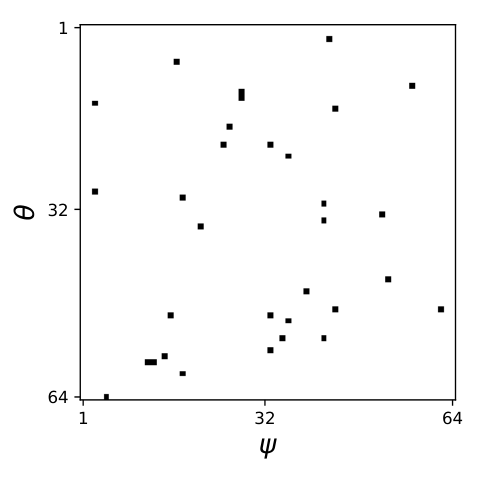
Once the posterior has converged sufficiently as described, we compute the inner 68th percentile range of the posterior, and locate the subset of training points within that range. The usage of the inner 68th percentile is a heuristic based on the amount of probability mass contained within for a normal distribution. We then test the sensitivity of the GP model predictions to each of the points in . We do this through “leave-one-out” validation. By this, we simply mean that the GP sensitivity to training point is computed by omitting from , re-computing a new GP surrogate from that down-sampled training set, and computing the -norm of the error between the new cost matrix predictions and the original. Once we have located that training point with the highest sensitivity, we add new training points in the vicinity of it, sampled at random from a Gaussian distribution centered at that point (these are denoted in Fig. 1). We then compute a new surrogate with this augmented training set, and continue with MOCU as before.
4 Examples and Results
We now proceed to apply surrogate-approximated MOCU to some example problems, in order to assess its performance in locating the optimal policy . To this end, we compute results for each example problem once using an adaptively refined surrogate, a second time using a static/non-refined surrogate, and a third time using full MOCU with no surrogates. We then compare how successful each method was in correctly locating the optimal policy. We also address other related topics, such as the rate of convergence of the uncertainty class distribution and how that is affected by the approximation scheme, and the qualitative properties of the method we use for computing sensitivity and adaptive refinement. In our examples, we show how our approximate MOCU methods may be used in a multifidelity setting, and how they may be applied to the design and control of physical systems.
4.1 Single Model Cost Function
Our goal here is to demonstrate our method on a fabricated cost function:
| (6) | ||||


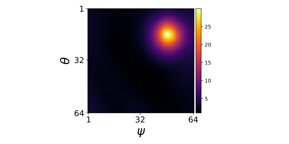
Fig. 2a displays a heatmap of this function for . We purposefully construct this cost function to have a long “ridge” of local minima, along with a relatively isolated global minimum. The reason for this is to introduce topography that might be missed by a surrogate constructed from too sparse of a data sampling. Given that coincides with the region around the global minimum, a relatively high degree of resolution in is needed to accurately predict the optimal strategy. We wish to explore how the isolated global minimum necessitates our adaptive sampling and refinement strategy when using a surrogate constructed from sparse data.
Regarding experimental design, we assume the following possible experiment space:
| (7) | ||||
One of the first issues that should be investigated is how our adaptive sampling criterion tends to perform on this problem. Fig. 2c shows the sensitivity computed with our leave-one-out strategy, averaged over 64 Monte Carlo realizations. For comparison, Fig. 2b shows the magnitude of the gradient of the cost function, approximated by finite-differencing GP surrogates and averaging over 64 Monte Carlo realizations. It is interesting that these results seem to indicate that even locally flat regions (e.g., very close to the global minimum) yield high sensitivity using the leave-one-out strategy. We believe this is due to sparse sampling: if, for instance, you only have one training point near the global minimum, removing that training point will strongly affect the surrogate, even though the local gradient is mild. For this reason, we might speculate that the leave-one-out strategy might provide a better measure of local “importance” than a gradient calculation when the important topography of the cost function in question involves isolated minima.
Fig. 3 shows an example of a surrogate that has been produced through adaptive refinement for this problem. We observe good selective refinement near the global minimum as desired. Fig. 4 shows an example of the OED results that are obtained using MOCU with adaptive surrogate construction for this problem. Initially, there is high entropy in the uncertainty class distribution, and the cost function is approximated with a coarse surrogate, so the computed policy is far from the optimal one. Eventually, once enough experiments have been conducted, the distribution over the uncertainty class collapses close to the correct value, and this triggers an adaptive refinement in the regions near . This results in training samples being added near the global minimum, which in turn results in a much closer approximation of the optimal policy.
Of course, the results shown in Fig. 3 and Fig. 4 are just one example. Because random sampling is involved in both constructing the initial surrogate and refining it, we need to conduct multiple independent Monte Carlo realizations to marginalize these effects out. Further, we need to do this for both the adaptive and non-adaptive schemes in order to confirm that the adaptive scheme actually provides some benefit. To highlight the effects of adaptivity, we also ensure that the total number of sample points used in the adaptive case never exceeds the total number used in the non-adaptive case. Thus, we use training points for each non-adaptive run; in the adaptive case, we construct the initial surrogate with training points and allow the option of adaptively refining twice with 8 points each time (for a total no higher than ).
Fig. 5 displays the evolution of with experiment for both the adaptive and non-adaptive cases and for full MOCU (i.e., MOCU conducted with access to the full cost function), averaged over 128 Monte Carlo realizations per method. We observe that, on average, all three methods give roughly the same convergence properties in . This suggests that in the MOCU method, epistemic uncertainty in is reduced at a rate that only weakly depends on the accuracy of the computed cost function . This may be a somewhat surprising observation, but it is one of the foundational insights to our approach. If indeed we will have to “wait” until a certain amount of experiments have been conducted before we have a good estimate of – and if this process is relatively unaffected by the use of an approximate – then it should be possible to use a cheaply-constructed surrogate for the cost function, and adaptively refine it only once we have conducted enough experiments.
Notwithstanding similarities in the evolution of among all methods, we do observe significant differences in the optimal policy calculation. Fig. 6 displays results related to the optimal policy recommendation. In this figure, we compute the average of the over the 128 Monte Carlo realizations at each experiment. We see that full MOCU obviously has the highest performance in locating the correct optimal policy (because it has access to the full cost function ). The rate at which it converges roughly mirrors the convergence of . This agrees with intuition in that the performance of full MOCU is limited by the rate at which one can reduce epistemic uncertainty through successive experiments. Regarding the two approximate schemes, we see that the adaptive method tends to outperform the non-adaptive one after a sufficient number of experiments have been performed (in this case, about 100). This is because the distribution of the uncertainty class has, on average, converged sufficiently by around 100 experiments that the adaptive refinement is triggered.
The comparison between full MOCU and the approximate schemes is interesting from a practical perspective, and the results suggest a trade-off between time spent evaluating the cost matrix and doing experiments. On one hand, each of the adaptive realizations used between and data points (i.e., the number of points in used to construct the surrogate), whereas a full MOCU realization required evaluations of the cost function. On the other hand, we see from Fig. 6 that full MOCU requires roughly an order of magnitude fewer experiments to achieve the same level of accuracy as adaptive MOCU required after 256 experiments. Even though the evolution of the uncertainty class distribution is almost identical for the two methods, full MOCU has access to the entire cost matrix and thus is more robust against larger amounts of uncertainty. The choice of whether to use our adaptive, surrogate-aided method over full MOCU will depend on how costly experiments are relative to evaluations of the cost matrix. If the cost matrix is very expensive to evaluate (e.g., a multiscale physics code) and experiments are inexpensive (e.g., there is a pre-existing repository of collected historical data and measurements), then one should consider using our approximate methods. If instead experiments are prohibitively expensive (e.g., a new exotic material must be fabricated and tested in a laboratory setting to yield a single measurement), then one should consider using regular, full MOCU.



4.2 Multiple Model Cost Function
Here, we extend the example from the previous section to a setting where there are two cost functions: one that computes an approximation of , and another that computes exactly. The motivation for introducing this is the problem of multifidelity models [9]. It is often the case that there are multiple computer models that all predict the same quantity-of-interest, but do so with computational expense inversely proportional to accuracy. In such a setting, we might wonder whether we could use the “cheap” approximate model to construct the initial surrogate, and then use samples from the “expensive” accurate model to refine the surrogate.
Fig. 7 displays the cheap/inaccurate and expensive/accurate cost functions used in this example. As can be seen, it is impossible to distinguish between the isolated minimum and the ridge minima on the basis of cost computed by the cheap model. It is therefore impossible for MOCU to compute the correct policy based on samples from the cheap model only; selective refinement from the expensive model is needed in the vicinity of the global minimum.
Fig. 8 reports Monte Carlo results for this case, using both adaptive and non-adaptive sampling and full MOCU. Note that both full MOCU and the non-adaptive surrogate-aided methods are done with respect to the expensive model only, so the results for those two cases are the same as in Fig. 6. Given the nature of this problem, we are mostly interested in how the adaptive algorithm compares with its non-adaptive counterpart. As has been noted, in the non-adaptive case, all training samples were drawn from the expensive model; in contrast, most samples for the adaptive case were drawn from the cheap model, with only a minority selectively drawn from the expensive model. And, as before, the total number of training samples for the adaptive case never exceeds the number used for the non-adaptive one (though it could be less). Even with these disadvantages, we observe that there is still statistically significant improvement in the optimal policy calculation using the adaptive method, which begins to become apparent after about 128 experiments.


4.3 Application: Coupled Spring-Mass-Damper Design
Here, we take a first step towards applying our methods to the design and control of physical systems. The problem setting will be a controls problem for a linear system. Specifically, we consider the following coupled spring-mass-damper system:
| (8) | ||||
We can recast this in first order form, along with an output QOI and control signal:
| (9) | ||||
In Eqn. 9, denote the displacements from equilibrium of the -springs, and denotes the 1-D velocities of these springs. In this problem, we let and , i.e. our input signal is a force that affects the first mass in the chain, and we are measuring the average spring displacement across the entire chain.
Our goal is to find the input sinusoidal signal that maximizes our output amplitude. This occurs at a resonant frequency of our system. For fixed system parameters, we can compute this from examination of the Bode magnitude plot of the transfer function from to , where and are the Laplace transforms of and . It is well-known that this transfer function – which we will denote as – can be computed as , where are the state-space matrices in Eqn. 9.
In our problem, we allow for uncertainty in the spring coefficients, and we wish to compute that sinusoidal forcing frequency that best maximizes the output amplitude, on average across this uncertainty. We note that one could use methods from optimal/robust control to solve this problem, instead of MOCU. Our goal in introducing this problem is simply to demonstrate our methods on a minimally-complex physical system.
Fig. 9a plots the Bode magnitude plot for the system with , in the range . We can clearly see the presence of a dominant resonant frequency as well as a secondary resonant frequency in this range. In this problem, we consider springs. We set and . We set the spring frequencies to , where is drawn from a uniform distribution: . Thus, our uncertainty class corresponds to increasingly stiff systems (up to the white noise produced by ). We also constrain the minimum allowable value of to 0.1. We take . The action set sets the forcing frequency of the input sinusoid: , where is a log-space mapping to the range . Fig. 9b displays an example ground-true cost function for this problem. Further, we set the true value of the uncertain parameter to be . We compute our cost function as ; that is, we compute the cost for a specific pair as the deviation in from the -specific maximum in . We note that this is a move one cannot make in a truly adaptive application (because it assumes one can calculate the maximum over for each ), but we simply do it here for convenience. In practice, one could circumvent this issue by instead considering an arbitrary reference point, for some , though that choice should not substantially affect the results for this problem.

We apply the same three MOCU methods to this problem as in the previous examples (i.e., non-adaptive and adaptive MOCU, with a surrogate for the cost function, and full MOCU). Note that in this problem, all surrogates (adaptive and non-adaptive) are initially constructed with 32 training points, and the adaptive surrogates are allowed two possible refinements of 8 points (for a total of 32 to 48 training points). Fig. 11 displays an example run of adaptively refined, surrogate-approximated MOCU for this problem, and Fig. 10 displays the statistical comparisons of the performance of full and approximate MOCU schemes. In comparing the two approximate methods, we find a predictable ranking: the adaptive method more accurately estimates the optimal policy with higher probability than the non-adaptive method. Regarding the full MOCU results, we observe the same trade-off that we noted previously: full MOCU can attain the same level of statistical accuracy as surrogate-approximated MOCU (or better), but with fewer needed experiments. As before, the decision of whether to use full MOCU or surrogate-approximated MOCU will depend on the relative cost of computation versus experimentation.
5 Conclusions
The goal of this research was to propose a new strategy for approximate OED for resource-constrained problems. Our motivation was to make OED (via MOCU) tractable for settings where the computational load needed to evaluate the design cost over the full set is prohibitively large. This could occur either because a single evaluation of is expensive for all pairs, or because the joint set is of large size, or both. Thus, our focus was on reducing the computationally-intensive stages of MOCU. To do this, we introduced the idea of using a surrogate model to approximate the cost function . This surrogate is built initially from sparsely-sampled data pairs drawn from , and it is refined adaptively as more information is gathered about the uncertainty class via the data-conditioned posterior . We applied this method to several example problems and examined its performance relative to a static, unrefined surrogate and full MOCU. We conclude that the adaptive refinement generally improves the performance of surrogate-driven approximate MOCU, but that the decision on whether to use full MOCU versus our approximate methods depends on the relative expense of evaluating the design cost versus doing an experiment, on the feasibility of doing full MOCU, and on the desired level of accuracy in optimal policy recommendations.
There are several avenues of further research that should be investigated in the future. One is practical: the approximation methods we have discussed should be applied to complex, “real-world” design problems. Another is theoretical: our methods are most useful in the case that experiments are inexpensive relative to compute-time. It would be useful to develop an extension that accounts for the relative expense of experiments and computations, and suggests a strategy that is weighted to account for this. For example, perhaps the number of initial training points and the number of adaptive refinements could be selected according to this criterion. One could also investigate how performance varies with different methods for adaptive selection (other than leave-one-out) and how the hyperparameters for our scheme might be tuned.
Funding Sources
This work was supported by the U.S. Department of Energy, Office of Science, Office of Advanced Scientific Computing Research, Mathematical Multifaceted Integrated Capability Centers program under Award Q1 DE-SC0019393.
Acknowledgments
We wish to thank Edward Dougherty, Byung-Jun Yoon and Nathan Urban for their helpful and insightful discussions on MOCU.
References
- [1] S. Boluki, X. Qian, and E. R. Dougherty, Experimental design via generalized mean objective cost of uncertainty, IEEE Access, 7 (2018), pp. 2223–2230.
- [2] X. Chen, Q. Lin, and D. Zhou, Optimistic knowledge gradient policy for optimal budget allocation in crowdsourcing, in International conference on machine learning, 2013, pp. 64–72.
- [3] R. Dehghannasiri, B.-J. Yoon, and E. R. Dougherty, Optimal experimental design for gene regulatory networks in the presence of uncertainty, IEEE/ACM Transactions on Computational Biology and Bioinformatics, 12 (2014), pp. 938–950.
- [4] R. Dehghannasiri, B.-J. Yoon, and E. R. Dougherty, Efficient experimental design for uncertainty reduction in gene regulatory networks, in BMC bioinformatics, vol. 16, Springer, 2015, p. S2.
- [5] P. Frazier, W. Powell, and S. Dayanik, The knowledge-gradient policy for correlated normal beliefs, INFORMS journal on Computing, 21 (2009), pp. 599–613.
- [6] P. I. Frazier, W. B. Powell, and S. Dayanik, A knowledge-gradient policy for sequential information collection, SIAM Journal on Control and Optimization, 47 (2008), pp. 2410–2439.
- [7] R. Ghanem and P. D. Spanos, Polynomial chaos in stochastic finite elements, (1990).
- [8] M. Imani, R. Dehghannasiri, U. M. Braga-Neto, and E. R. Dougherty, Sequential experimental design for optimal structural intervention in gene regulatory networks based on the mean objective cost of uncertainty, Cancer informatics, 17 (2018), p. 1176935118790247.
- [9] B. Peherstorfer, K. Willcox, and M. Gunzburger, Survey of multifidelity methods in uncertainty propagation, inference, and optimization, Siam Review, 60 (2018), pp. 550–591.
- [10] I. O. Ryzhov, W. B. Powell, and P. I. Frazier, The knowledge gradient algorithm for a general class of online learning problems, Operations Research, 60 (2012), pp. 180–195.
- [11] C. K. Williams and C. E. Rasmussen, Gaussian processes for machine learning, vol. 2, MIT press Cambridge, MA, 2006.
- [12] D. Xiu and G. E. Karniadakis, The wiener–askey polynomial chaos for stochastic differential equations, SIAM journal on scientific computing, 24 (2002), pp. 619–644.
- [13] B.-J. Yoon, X. Qian, and E. R. Dougherty, Quantifying the objective cost of uncertainty in complex dynamical systems, IEEE Transactions on Signal Processing, 61 (2013), pp. 2256–2266.
- [14] B.-J. Yoon, X. Qian, and E. R. Dougherty, Quantifying the multi-objective cost of uncertainty, arXiv preprint arXiv:2010.04653, (2020).