HRI-RECAPP-2020-10
A relatively light, highly bino-like dark matter in the -symmetric NMSSM and recent LHC searches
Abstract
A highly bino-like Dark Matter (DM), which is the Lightest Supersymmetric Particle (LSP), could be motivated by the stringent upper bounds on the DM direct detection rates. This is especially so when its mass is around or below 100 GeV for which such a bound tends to get most severe. Requiring not so large a higgsino mass parameter, that would render the scenario reasonably ‘natural’, prompts such a bino-like state to be relatively light. In the Minimal Supersymmetric Standard Model (MSSM), in the absence of comparably light scalars, such an excitation, if it has to be a thermal relic, is unable to meet the stringent experimental upper bound on its abundance unless its self-annihilation hits a funnel involving either the -boson or the Standard Model (SM)-like Higgs boson. We demonstrate that, in such a realistic situation, a highly bino-like DM of the popular -symmetric Next-to-Minimal Supersymmetric Standard Model (NMSSM) is viable over an extended range of its mass, from our targeted maximum in the vicinity of the mass of the top quark down to about 30 GeV. This is facilitated by the presence of comparably light singlet-like states that could serve as funnel (scalars) and/or coannihilating (singlino) states even as the bino-like LSP receives a minimal (but optimal) tempering triggered by suitably light higgsino states that, in the first place, evade stringent lower bounds on their masses that can be derived from the Large Hadron Collider (LHC) experiments only in the presence of a lighter singlino-like state. An involved set of blind spot conditions is derived for the DM direct detection rates by considering for the very first time the augmented system of neutralinos comprising of the bino, the higgsinos and the singlino which highlights the important roles played by the NMSSM parameters ‘’ and in delivering a richer phenomenology.
Keywords
Supersymmetry Phenomenology1 Introduction
It is well-known in the context of the Minimal Supersymmetric extension of the Standard Model (MSSM) that a pure bino () neutralino as the Lightest Supersymmetric Particle (LSP; ) and a Weakly Interacting Massive Particle (WIMP) could be a viable cold Dark Matter (DM) candidate, which is a thermal relic, under two specific situations: (i) if it is lighter than GeV and some sfermions (in particular, the right-handed sleptons with large hypercharge coupling; such light squarks being ruled out long back) are not much heavier than 100 GeV such that the so-called bulk (-channel) annihilation of a pair of DM states mediated by such sfermions are optimally efficient ArkaniHamed:2006mb; Pierce:2013rda; Fukushima:2014yia; Baum:2020gjj and/or (ii) if there is an efficient coannihilation of such a DM state with slepton(s) () with GeV when the sleptons are degenerate Chakraborty:2019wav; Ellis:1999mm. However, requiring such a pure bino DM (the lightest neutralino, ) to be relatively light, i.e., GeV, both the possibilities are found to be practically ruled out by the Large Hadron Collider (LHC) experiments Aad:2019vnb; Aad:2019qnd save for the cases with light staus with comparable mass Aad:2019byo. Such a situation, keeping up further with the ever-improving lower bounds on the sparticle masses, has prompted studies where sleptons are assumed to be rather heavy Huang:2017kdh; Badziak:2017the; vanBeekveld:2016hbo; Abdughani:2017dqs. Thus, in the framework of the MSSM, only a tempered bino-dominated LSP, with optimal admixtures of higgsinos Feng:2000gh; Baer:2005bu and/or wino Masiero:2004ft; Baer:2005zc; Baer:2005jq; BirkedalHansen:2001is; BirkedalHansen:2002am, fits the bill so far as compliance with the experimentally observed upper bound on the DM relic abundance Ade:2015xua; Aghanim:2018eyx is concerned which may be ensured in the presence of resonant self-annihilations (funnels) or efficient coannihilation of the DM particles.
On the other hand, stringent and improved upper bounds on spin-independent (SI) Aprile:2018dbl and spin-dependent (SD) Aprile:2019dbj; Amole:2019fdf DM-nucleus (elastic) scattering cross sections that are routinely arriving from various DM Direct Detection (DMDD) experiments could genuinely motivate a nearly pure bino DM. In fact, such bounds coming from the SI experiments tend to be the most stringent ones when the DM mass is relatively low, around or below 100 GeV Aprile:2018dbl. This could prompt one to suspect a nearly pure bino-like DM hiding in this mass-range. It may further be noted that the excess of -ray emanating from the galactic center as observed by an indirect DM-detection experiment like the Fermi-LAT experiment TheFermi-LAT:2017vmf; Fermi-LAT:2016uux can also be explained in terms of a (relatively light) bino-dominated DM Agrawal:2014oha; Freese:2015ysa; Butter:2016tjc; Achterberg:2017emt.
In the absence of optimally light sleptons, a scenario that has been discussed in a preceding paragraph, the only ways such a highly bino-like DM of the MSSM could comply with the upper bound on its relic abundance are the following: (i) presence of an efficient -channel mutual annihilation funnel, e.g., in the form of a resonant - or a Higgs boson with or , respectively and/or (ii) possibility of coannihilation of the DM neutralino with other electroweakino(s) (the ewinos, i.e., the charginos and the neutralinos) close in mass to the DM state. Furthermore, note that for such a light DM, their otherwise prolific annihilations to a pair and to a pair can both be closed. Compliance with the reported upper bound on its relic abundance thus gets even more challenging.
In any case, in the framework of the MSSM, an efficient enough resonant (funnel) annihilation or a coannihilation process mentioned above necessarily requires some minimal higgsino and/or wino admixture in the otherwise bino-like LSP DM. Note that for funnels involving -boson and the SM-like Higgs boson (), the mass of the annihilating LSP gets almost discretely fixed to either or , respectively. Given current lower bounds on the masses of the heavier MSSM Higgs states ( GeV) Aaboud:2017sjh; Sirunyan:2018zut; Bahl:2018zmf; Aad:2020zxo, those cannot provide funnels for self-annihilation of the LSP DM with mass GeV which is in our focus. On top of that, bounds on SD rates put a stringent bound on the higgsino mass parameter ‘’ ( GeV) which in turn rules out a possible higgsino-like Next-to-LSP (NLSP) having a mass lighter than that Carena:2018nlf. In addition, recent LHC studies Aad:2019qnd; Aaboud:2017leg also appear to put a bound GeV on lighter, nearly degenerate ewinos. These together stand in the way for an LSP with mass GeV coannihilating with a close by ewino state Calibbi:2014lga.
The situation is different in a crucial way, in the Next-to-MSSM (NMSSM) Ellwanger:2009dp, a popular extension of the MSSM. In the NMSSM, the so-called -term () in the superpotential is replaced by a term , where is a chiral superfield and a singlet under the Standard Model (SM) gauge group and ‘’ is a dimensionless coupling much akin to a Yukawa coupling. The presence of gives rise to a singlet scalar field ‘’. An effective ‘-term’ () is generated dynamically when ‘’ acquires a vacuum expectation value (vev) such that thus offering a possible solution to the infamous -problem Kim:1983dt that plagues the MSSM. The NMSSM Higgs sector possesses two extra singlet scalar states of -even () and -odd () varieties when compared to the MSSM. In addition, a singlet Majorana fermion, the ‘singlino’, augments the MSSM neutralino sector.
Such a spectrum is known to influence both DM and collider phenomenology in a nontrivial way, in particular, in a -invariant version of the NMSSM with its free (input) parameters being arbitrary at the weak scale (the so-called phenomenological NMSSM or the pNMSSM). Scenarios with light higgsinos and a singlino, in which either of them could turn out to be the LSP (DM), and accompanied by one or more light singlet-like scalars, have attracted much attention since the early days of the NMSSM scenario. This has surely been driven by the existence of nontrivial couplings among the singlet-like states (the singlino and the singlet scalars) and the doublet-like ones (the MSSM-like Higgs bosons and the higgsinos) that characterize the NMSSM.
In comparison, dedicated, general studies on a possible bino-dominated DM in the NMSSM are lacking. This is presumably since the NMSSM does not suggest any direct tree-level coupling among the bino and the new singlet states that it offers thus leaving the pertinent setup, to a good extent, appearing like one with only the bino and the higgsinos (and the wino) of the MSSM Beskidt:2017xsd. However, for a highly bino-like LSP DM, which is in the focus of the present work, the much important phenomenon of DM annihilation could find a crucial, additional boost in the presence of possibly light singlet-like scalar states Belanger:2005kh; Gunion:2005rw (in particular, even lighter than the -boson) which might act as funnels over an extended range of DM masses, even below . Some later studies Das:2010ww; Vasquez:2010ru; Cumberbatch:2011jp; Han:2014nba concentrated on a light bino-like DM ( GeV, down to a few hundreds of MeV) that funnels through such light scalar(s) and were mostly motivated by the then recent reported excesses at experiments like DAMA, CoGeNT and CDMS-II and the exclusion limits from XENON and CDMS-Si experiments which all seemed to be compatible with such excesses. Furthermore, the mentioned -ray excess as observed by the Fermi-LAT experiment also seems to fit better with a not so heavy bino-like DM of the NMSSM when compared to the MSSM, in the presence of light singlet scalars Cheung:2014lqa; Guo:2014gra; Gherghetta:2015ysa; Bi:2015qva; Cao:2015loa; Shang:2018dja. Phenomenological studies of efficient search-strategies of such light scalars (irrespective of the nature of the LSP) have remained to be an active enterprise Dermisek:2005ar; Christensen:2013dra; Cerdeno:2013qta; Cao:2013gba; King:2014xwa; Dutta:2014hma; Bomark:2015fga; Ellwanger:2015uaz; Conte:2016zjp; Guchait:2016pes; Baum:2017gbj; Guchait:2017ztk; Ellwanger:2017skc; Baum:2019uzg; Barducci:2019xkq; Guchait:2020wqn while their actual searches constitute a dedicated and a vibrant programme at the LHC Aaboud:2018fvk; Aaboud:2018gmx; Aaboud:2018iil; Aaboud:2018esj; Aad:2020rtv; Sirunyan:2018mbx; Sirunyan:2018mot; Sirunyan:2020eum.
During recent years, the phenomenology of a bino-dominated neutralino DM in the pNMSSM has been discussed as parts of some general studies, in different contexts in refs. Baum:2017enm; Cao:2018rix; Domingo:2018ykx. For example, the analysis in ref. Baum:2017enm focuses on the region of parameter space that does not bank on large radiative corrections to find the mass of the SM Higgs boson in the proximity of its observed value of 125 GeV (and hence can be called a ‘natural’ scenario) and, at the same time, the Higgs sector is attributed with the so-called ‘alignment-without-decoupling’ Carena:2015moc; Baum:2017gbj; Baum:2020vfl. Compliance with these two conditions together, for the doublet Higgs states, requires and . The study rules out a bino-like DM lighter than the top quark. Ref. Cao:2018rix, on the other hand, allows for relatively light sfermions that help achieve the right relic abundance via their coannihilation with the neutralino DM. The work infers that a bino-like DM in a ‘natural’ pNMSSM setup is strongly disfavored by results from various DM and the LHC experiments. Ref. Domingo:2018ykx instead performs a study with the then latest LHC results (with expressly less prejudice towards the DM-related issues) to shed light on the fate of a bino-dominated DM within the pNMSSM where the wino- and the higgsino-like states are mostly on the lighter side ( GeV) while the singlino-like one could be as light as GeV. Thus, in that study, all such states could play the role of the NLSP and the LSP can have significant wino and higgsino admixtures.
In this backdrop, in the present work, we study in detail the viability of a highly bino-like DM (with bino content %) of the pNMSSM with mass below GeV (and, in particular, below GeV) vis-a-vis the theoretical and the current experimental constraints. The wino is taken to be much heavier.11 1 A heavy wino straightaway aids compliance with the stringent lower bounds on the masses of the wino-like states as reported by the LHC experiments. Furthermore, this precludes their presence in the cascades of lighter ewinos thus rendering the scenario much less cluttered for our present analysis of a bino-higgsino-singlino system. Thus, we allow for up to 5% tempering (a somewhat ‘minimal’ tempering) of the bino-like LSP DM by the higgsinos and the singlino. We then open ourselves up to a broader region of the NMSSM parameter space, mainly by allowing for smaller values of ‘’ and a larger range of , when compared to ref. Baum:2017enm. Furthermore, we consider the sleptons to be much heavier when compared to ref. Cao:2018rix such that bulk annihilation and coannihilation of the DM involving sleptons can no more be instrumental. The squarks and, in particular, the top squarks are assumed to be rather heavy (beyond the reach of the LHC). The latter choice might result in some compromise on ‘naturalness’ (or ‘finetuning’) Ellis:1986yg; Barbieri:1987fn. The situation could be ameliorated by restricting to smaller values ( GeV) as has been advocated in the recent past Baer:2012up; Baer:2013ava; Mustafayev:2014lqa; Baer:2015rja. This opens up the interesting possibility of relatively light higgsinos Jeong:2014xaa just heavier than a singlino-like NLSP, the rich phenomenology of which we would discuss in detail. An MSSM-like scenario with a lighter higgsino-like NLSP (while the LSP is still bino-like) is also viable and we would briefly comment on it in the pNMSSM context.
However, a relatively small is restricted by both DMDD experiments Carena:2018nlf and from the LHC constraints on the invisible decay width of Arbey:2012na.22 2 Naively, since bino-higgsino mixing is driven by the gauge coupling , a bino LSP could allow a somewhat lower value of without getting into conflict with these constraints when compared to the singlino LSP whose mixing with higgsinos is governed by ‘’ which is generally larger than in the phenomenologically interesting region of the parameter space. On top of that, GeV seems to be getting into a soaring tension with the null results from the direct searches of ewinos at the LHC in the modes followed by their exclusive decays to SM gauge and Higgs bosons Sirunyan:2017lae; Sirunyan:2018ubx; Aaboud:2018jiw; Aaboud:2018sua; Aaboud:2018ngk; Aad:2019vnb; Sirunyan:2019iwo; Aad:2019vvf; Aad:2019vvi; Aad:2020qnn; ATLAS:2020ckz, viz.,
| (1) | |||||
In the MSSM context, some recent studies Calibbi:2014lga; Chakraborti:2014gea; Chakraborti:2015mra; Athron:2018vxy; Datta:2018lup have taken a critical look into the robustness of such constraints when these states are higgsino-like. Their production rates at the LHC are known to be smaller than the wino-like states of the same mass. This would result in a commensurate degradation of the experimental reach for such states. On top of that, a further degradation in sensitivity is unavoidable if the cascades of such states follow patterns that are different from the simplistic ones assumed by the LHC experiments. This is indeed possible in the NMSSM. We thus focus on the region of the parameter space where the concerned ewinos undergo cascades that involve NMSSM excitations (e.g., the singlet scalars or the singlino) that either compete with or dominate over the MSSM-like ones (involving the -boson and ). These then result in relaxed bounds on the masses of such higgsino-like states () Ellwanger:2018zxt; Domingo:2018ykx; Abdallah:2019znp thus making a smaller still viable.
As we will see, the interplay of DM and collider phenomenology for such a DM state is a highly involved phenomenon. Contrary to an expectation naively guided by what happens in the MSSM, the pNMSSM scenario indeed allows for a highly bino-like DM over a broad range of its mass below GeV and over a significant region of the NMSSM parameter space, even when the sfermions are decoupled. In the process, a crucial role in the DM sector is played by larger values of (). On the one hand, this enhances the interaction between a singlet scalar, and/or (predominantly, ) and a bottom quark pair thus facilitating DM annihilation over an extended range of its mass dictated by the mass of the singlet scalar state, i.e., . On the other hand, as we will see, for smaller DM masses only such larger values of could optimally tame the SI scattering rate of the DM by arranging for a so-called ‘blind spot’ in the collective contribution of -even scalars to the same. The other crucial parameter is ‘’. A moderate to large value of ‘’ () is found to play a deciding role in relaxing the LHC bounds on optimally in the presence of a singlino-like NLSP so that a ‘minimal’ but an adequate tempering of a bino LSP with higgsino (and hence singlino) admixture stands feasible down to smaller DM masses.
The paper is organized as follows. In section 2 we outline the theoretical setup by summarizing the salient features of the NMSSM superpotential and its scalar and ewino sectors. To set the stage, the interplay of the scalars and the ewinos, in terms of correlations among their masses and interactions, is then discussed in necessary details, with a bino-like LSP in mind. Section 3 presents the main results of this work by referring to the phenomenology of DM relic abundance, its Direct Detection (DD) rates and some interesting collider aspects of such a scenario. Their collective implications for the future DMDD and the LHC experiments are also indicated. We present a few benchmark scenarios that capture the salient aspects of the involved phenomenology. Further, a brief observation is made on the issue of ‘naturalness’ in the light of the findings of this paper. In section 4 we conclude. A three-part appendix is presented at the end by (i) including the general form of the scalar-neutralino-neutralino interactions in a convenient basis and to be exploited later, (ii) presenting for the very first time relevant results pertaining to the SI and the SD blind spots calculated in the bino-higgsino-singlino basis and finally (iii) discussing -dependence of the relevant ewino partial widths in terms of the involved couplings that would help in understanding the deeper mechanism of how a small could evade pertinent LHC bounds.
2 The theoretical scenario
The superpotential of the -symmetric NMSSM is given by Ellwanger:2009dp
| (2) |
where is the MSSM superpotential without the higgsino mass term (the so-called -term), are the Higgs doublet superfields of the MSSM while is the gauge singlet superfield of the NMSSM. ‘’ and ‘’ are dimensionless coupling constants for the interaction among the doublet and the singlet fields and the self-interaction of the singlet field, respectively. As the singlet scalar field, ‘’ develops a vacuum expectation value (vev) , the second term in eq. (2) gives rise to an effective -term given by thus offering a solution to the baffling -problem Kim:1983dt. The corresponding soft supersymmetry (SUSY)-breaking Lagrangian is given by
| (3) |
where the first term on the right-hand side gives the soft part of the MSSM Lagrangian but for a vanishing soft term () of the MSSM containing the higgsino mass parameter ‘’ while stands for the soft SUSY-breaking mass of the singlet scalar field, ‘’ and and are the trilinear soft terms of the NMSSM with the dimensions of mass. The singlet superfield also yields a fermionic partner known as the singlino. Together, these constitute the defining aspects of the scalar (Higgs) and the chargino/neutralino (ewino) sectors of the NMSSM that directly concern the present work. Hence we briefly discuss the structure and the salient features of these two sectors in the subsequent subsections.
2.1 The scalar (Higgs) sector
The Lagrangian of eq. (3) contains the following soft Lagrangian for the NMSSM Higgs sector that now includes soft masses and couplings specific to the NMSSM, over and above the relevant MSSM terms:
| (4) |
Perturbative calculations would involve expansion of the Lagrangian about the real vev’s of the neutral Higgs fields (, ) and the neutral gauge-singlet scalar field (), i.e., , and . Thus,
| (5) |
where ‘’ and ‘’ stand for the -even and the -odd states. The symmetric squared mass matrix for the -even scalars in the basis is given by Ellwanger:2009dp
| (6) |
where , , and are the and gauge couplings, respectively, and , such that GeV)2 and . The -even (scalar, ) mass eigenstates are then given by
| (7) |
where the matrix ‘’ diagonalizes .
For the -even scalars, it is, however, more convenient to work in a rotated basis () Miller:2003ay; Badziak:2015exr where , and . This is since now mimics the SM Higgs (heavy MSSM (doublet)-like -even Higgs) field. The physical -even scalar states are then denoted by
| (8) |
where is the matrix that diagonalizes the mass-squared matrix for the -even scalars in the rotated basis. To be more specific, stands for the admixture of the ‘’-th scalar state in the ‘’-th physical state. The symmetric squared mass matrix for the -odd scalars in the basis is given by Ellwanger:2009dp
| (9) |
For , a similar rotation, as used in the -even case, of the doublet basis states and would project out the massless Nambu-Goldstone mode that can be dropped. The orthogonal state is identified as the MSSM (doublet)-like -odd (pseudoscalar) Higgs boson and in the basis the mass-squared matrix for the -odd scalar is reduced to
| (10) |
where, akin to that in the MSSM, . The -odd (pseudoscalar, ) mass eigenstates are given by
| (11) |
where the matrix ‘’ diagonalizes . The elements of the matrix ‘’ and the matrix ‘’ that diagonalizes are related by Ellwanger:2009dp
| (12) |
The -odd mass eigenstates in terms of the basis are then given by
| (13) |
At tree-level, modulo possible mixing with the doublet states and (the so-called singlet-doublet mixing), the squared mass of the singlet-like -even physical state is given by the (3,3) component of , i.e.,
| (14) |
Furthermore, while the mass of the heavier of the two MSSM (doublet)-like -even neutral physical states, , is given by (), the squared mass of the lighter one mimicking , at one-loop level, is given by Ellwanger:2011sk
| (15) |
In the above expression, the first and the second terms stand for the tree-level MSSM and NMSSM contributions, respectively, while stems from a possible singlet-doublet mixing and, in the weak mixing limit (as is now favored by the LHC data), is given by Ellwanger:2011sk
| (16) |
where and . The term gives the MSSM-like radiative corrections to of which the dominant one at one-loop level, with the top quark and the top squarks (stops) in the loops, is given by Haber:1996fp; Djouadi:2005gj
| (17) |
where stands for the mass of the SM top quark, , being the mass of the lighter (heavier) physical top squark state and , being the soft trilinear coupling for the top sector. On the other hand, the squared mass of the singlet -odd scalar, up to some mixing with its doublet cousin, is given by
| (18) |
Eqs. (14), (15) and (18) indicate nontrivial dependencies of the masses of the singlet scalars and the SM-like Higgs boson on various input parameters of the -symmetric pNMSSM. For example, as is well-known, could be either heavier or lighter than and the mass of the latter is not always strongly correlated with the mass of its -odd counterpart, , although both are singlet states having a common origin. As we will find, such correlations (or, for that matter, their absence) could crucially govern their collective phenomenology.
2.2 The ewino sector
As in the MSSM, the ewino sector of the NMSSM is comprised of the neutralino and the chargino sectors with the exception that the former is now augmented with a singlino () state, the singlet fermionic degree of freedom that owes its origin to the gauge-singlet superfield appearing in the NMSSM superpotential indicated in eq. (2). As a result, the symmetric neutralino mass matrix has got a dimensionality of and, in the basis , is given by Ellwanger:2009dp
| (19) |
where and are the soft SUSY-breaking masses for the and the gauginos, i.e., the bino and the wino, respectively, while the same for the singlino, appearing in the (5,5) element, is given by . The neutralino mass-eigenstates (, , in order of increasing mass as ‘’ increases), in terms of the weak eigenstates (, with ), are given by
| (20) |
where ‘’ is the matrix that diagonalizes the neutralino mass-matrix in eq. (19).33 3 We would finally work with a neutralino system where the wino is decoupled. For the resulting system, various useful relations among ’s are given explicitly in appendix B.
On the other hand, the () chargino mass matrix of the NMSSM is same as that of the MSSM but for and, in the bases and , is given by Ellwanger:2009dp
| (21) |
The asymmetric matrix can be diagonalized by two () unitary matrices ‘’ and ‘’:
| (22) |
In this work, we focus on a scenario where the LSP DM is a highly bino-like neutralino. As noted in the Introduction, to make sure that our setup remains reasonably ‘natural’, we focus on relatively low values of , subject to its current lower bounds from the experiments. A priori, this yields two relatively light higgsino-like neutralinos along with a higgsino-like lighter chargino with masses . Also, we would assume a decoupled wino, i.e., a large . This would keep the analysis simpler without having to forego any of its major features by prohibiting wino(s) in the cascades of heavier ewinos and, at the same time, by aiding compliance with stringent bounds on the former by rendering their direct production rate small enough at the LHC.44 4 The combined cross section for the associated production of wino-like charginos and a wino-like neutralino at the LHC energies is roughly twice as large the combined one for higgsino-like charginos and higgsino-like neutralinos of which there are two nearly degenerate states Ellwanger:2018zxt.
The NMSSM-specific effects in the ewino sector get to be rather interesting when the soft singlino mass becomes comparable to both and . It may be gleaned from eq. (19) that the mixings of the singlino with the higgsinos are governed directly by ‘’ while its mixing with the bino is absent. At the lowest order, such a mixing only occurs through the higgsino portal, though the same can get enhanced for . Furthermore, depending on whether or , the NLSP would be singlino- or higgsino-dominated. Note that, in the latter case, the neutralino sector reduces to a typical bino-higgsino system of the MSSM when the singlino also gets decoupled. In any case, the actual masses and contents of various neutralinos depend much on the extent of mixing among various states and could be critically important for both DM and collider phenomenologies.
The setup under consideration thus has one light chargino which is higgsino-like and four relatively light neutralinos with the lightest one of them (the LSP) being bino-like while the others are singlino- and higgsino-like. If the higgsino-like neutralinos are lighter than the singlino-like one (while the wino is decoupled), phenomenology at the collider (LHC) would mostly resemble an MSSM scenario with a higgsino-like NLSP except under a situation when the mass-split between the higgsinos and the LSP is rather small Dutta:2014hma. However, the phenomenology of the DM sector might still be somewhat sensitive to a not so heavy singlino-like state given even a small admixture that it could lend to the bino-like LSP neutralino. On the other hand, a singlino-like NLSP might affect the collider phenomenology as well since higgsinos, which could be copiously produced at the colliders, can now cascade to the former. This implies that the stringent lower bounds on the masses of such ewinos that could be placed by different LHC analyses within the framework of simplified SUSY scenarios might get significantly relaxed thus warranting thorough reanalyses that admit such possibilities.
2.3 The interplay of the scalars and the ewinos
The interplay of the relatively light scalars and the ewinos is known to be central to the DM and the collider phenomenologies alike in the -symmetric pNMSSM scenario. In ref. Abdallah:2019znp we highlighted some of the crucial aspects of such an interplay in the context of a scenario with a singlino-dominated LSP. The study presented here has an unmistakable parallel to that but with a flipped mass-hierarchy between the singlino- and the bino-like states. Nonetheless, there are crucial quantitative differences which may not be unexpected.
As is common to a scenario with a single SUSY DM candidate, the one under consideration is also plagued with a tension between the observed values of relic abundance and the upper bound on the DMDD cross section. Similar to what happens in the MSSM, a pair of pure bino LSPs cannot funnel via - or the Higgs boson as those do not couple to the latter two states. Furthermore, its efficient coannihilations with a sfermion and/or an ewino are also not possible if we assume the latter ones to be much heavier than the LSP. Thus, for a light enough bino-like LSP (say GeV), the only way it could become a viable DM candidate is if it acquires some higgsino admixture and if or .55 5 The -funnel region in the MSSM, in general, is nearing complete exclusion due to various recent experimental constraints on the DM sector and those coming from searches for the ewinos at the LHC Pozzo:2018anw; Barman:2020zpz. This is true in the NMSSM as well but now with a further possibility that the SM-like Higgs funnel could get efficient if, in addition, there is some singlino admixture in the LSP. Notably, there could be additional funnels available thanks to relatively light singlet-like scalars of the NMSSM which can be either heavier than or lighter than the -boson or could even have a mass in between and . However, the tension shows up in the form that if efficient scalar (Higgs) funnels are to be banked on for compliance with the observed DM relic abundance, the SI cross section tends to breach the upper bound on it. This is since the same interactions (--) govern these two phenomena. On the other hand, a similar problem arises with the SD cross section when the -funnel is in action both of which are governed by the -- couplings.
Ramifications of such a scenario at the collider experiments primarily depend on the altered branching ratios of the heavier ewinos to the lighter ones (that include the LSP) in the presence of light singlet-like scalars and/or a singlino-like neutralino. As pointed out in the Introduction, a multitude of LHC constraints in the form of bounds on the masses of the ewinos, derived assuming so-called ‘simplified models’ within the framework of the phenomenological MSSM (pMSSM), could now get significantly relaxed. In particular, such relaxations for the higgsino-like ewinos could open up the parameter space with relatively low values of and hence with improved ‘naturalness’. In our present scenario in which all sparticles but for the bino- and the singlino-dominated neutralinos, the higgsino-dominated neutralinos and chargino and the low-lying doublet- and singlet-like scalars (both of -even and -odd variants) are taken to be too massive and hence decoupled, the relevant decay branching ratios are mostly governed by the interactions of the heavier neutralinos to their lighter cousins and the scalar states (--) and the -boson (--). These are the very same interactions that we have discussed in the previous paragraph in the context of DM phenomenology. Furthermore, interactions involving the lighter chargino, the neutralinos lighter than the same and the -boson, --, could also be rather instrumental. In fact, situations exist when the lighter chargino, whose decay branching ratio to the -boson and the LSP is usually considered to be 100% by the LHC experiments, could have a reasonable branching ratio to a neutralino other than the LSP and a -boson. This could potentially relax the published experimental bounds further.
Clearly, the following few issues would primarily set the contour of the interplay between the scalar (Higgs) and the ewino sectors in the current context: (i) masses of the singlet-like scalars, (ii) the same masses and the observed masses of the -boson and the SM-like Higgs boson in relation to those of the bino-like LSP and the other ewinos, (iii) mass-splittings among the ewinos themselves including the LSP and (iv) compositions of the LSP and the other ewinos. All of these have intricate dependencies on various input parameters of the pNMSSM. In the subsequent subsections, we highlight the mass-correlations that exist among the singlet-like states and the interactions among the scalars, the ewinos (that include both singlet and doublet states) and the SM gauge boson.
2.3.1 Correlations among masses of the scalars and the ewinos
Correlations among masses of the Higgs-like states and the neutralinos (higgsino- and singlino-like) have recently been studied in some detail in ref. Baum:2019uzg in the so-called alignment (without decoupling) limit Carena:2015moc; Baum:2017gbj; Baum:2020vfl which allows for relatively light non-SM Higgs states (-even/odd, singlet/doublet), i.e., with masses TeV and hence are likely to be within the reach of the LHC. However, the said work studies such correlations in a ‘natural’ setup for which MSSM-like radiative corrections to the SM-like Higgs mass have to be, at best, moderate while the tree-level NMSSM contribution () to the same is maximized by choosing relatively large values of ‘’ () and by restraining to low values (). In contrast, as pointed out in the Introduction, we open our scans to regions with smaller values of ‘’ as well. Furthermore, we look for relatively light singlet-like scalar states ( GeV) while the non-SM doublet scalars (MSSM-like heavier Higgs states) are taken to be indeed heavy ( TeV) and hence decoupled. These requirements, in contrast to the scenario discussed in ref. Baum:2019uzg, would render the mass-correlation among the corresponding heavy and light eigenstates relatively milder. Under the circumstances, the correlations among the masses of the light singlet states (scalars and the singlino) assume importance and worth a closer look.
The masses of the -even singlet and the doublet (SM Higgs boson) and that of the -odd singlet scalars as described by eqs. (14), (15) and (18) along with the mass of the singlino appearing as the (5,5) element of the neutralino mass matrix of eq. (19) present us with a rich set of observables whose values are intricately correlated. Such correlations have an important bearing on the phenomenology and their understanding is paramount for its systematic study. Generally, there are two crucial implications of such correlations. First, the masses of these singlet-like scalars and the singlino-dominated state control the DM physics in a rather involved manner by influencing both DM relic abundance and DMDD rates. Second, the mass-hierarchy among these states would dictate their decay patterns and hence what to expect at a collider like the LHC.
As can be seen from eqs. (14) and (18), the masses of the singlet-like scalars, at the lowest order, have rather involved dependencies on as many as six input parameters like , , , , and while masses of the neutralinos have relatively simpler (well-known) dependencies on the first four of them plus that on the two soft masses and . Thus, it is not quite unexpected that the masses of the singlet scalars and the singlino would be correlated. In fact, in the so-called decoupling limit with or for a sizable and small ‘’, ‘’ and for which mixing among the singlet and doublet scalars can be ignored, the following sum-rule holds Das:2012rr; Ellwanger:2018zxt:
| (23) |
where () is the mass of the singlet-like -even (odd) scalar excitation.
Scatter plots in figure 1 present the correlations among the masses of the singlet-like -even and -odd scalars and the singlino-like neutralino (left panel) and illustrate to what extent these masses conform to the sum-rule presented in eq. (23) (right panel). These result from a scan, using the package NMSSMTools-v5.4.1 Ellwanger:2004xm; Ellwanger:2005dv; Das:2011dg, over various pNMSSM parameters the ranges of which are indicated in table 1.


It can be found from the left plot of figure 1 that for larger values of , . This (up to some higher order corrections as incorporated in NMSSMTools), already follows from the lowest order expression of in eq. (14) given that the magnitude of (in the second term) never gets large in our scan ( GeV) and that the first term being proportional to (as ) may be ignored when ‘’ is on the smaller side. Also, for any given value of there is a maximum possible value of determined by the largest value of in use as mentioned above. In fact, the maximum attainable gets to be increasingly smaller when compared to the corresponding value of . This can be understood from eq. (18) when ‘’ is small (note that this is the limit in which the sum-rule of eq. (23) is obtained), for which the first term in the same could be ignored and hence . We have checked that the sharper edge in the distribution (which divides the plot into a dense red region at the bottom and a sparse region in green above) indeed satisfies this relation. In fact, the latter region corresponds to larger ‘’ values.
| Varying parameters | (TeV) | (TeV) | (GeV) | (GeV) | (TeV) | |||
| Ranges | 0.001–0.7 | 0.7 | 1–65 | 10 | 200 | 0–10 |
The situation is, however, different for smaller values of ( GeV) when the first and the third terms in eq. (18), which are initially ignored, could turn out to be comparable in magnitude with the second term. This allows for for such low values of . A little loosely connected patch at the bottom, left corner is the only region populated to a certain extent by points for which where even the singlet-like -odd scalar could be heavier than its -even counterpart. We have checked that this region extends over and . Over this region tends to drop as increases for a given with at smaller (larger) .
One crucial information from this plot is that one can have a light enough while and the singlino-like neutralino could be much heavier. An important implication of such a spectrum is that the DM annihilation could just take advantage of an -funnel which would need only some higgsino admixture in the LSP while the SI cross section does not receive much contribution from a heavy enough . Note that the bottom part of this plot is sparsely populated. This is since over this region which allows for the decay and hence attracts significant constraint from the LHC experiments Aaboud:2018fvk; Aaboud:2018gmx; Aaboud:2018iil; Aaboud:2018esj; Aad:2020rtv; Sirunyan:2018mbx; Sirunyan:2018mot; Sirunyan:2020eum.
The right plot of figure 1 presents the distribution of the scatter points in a plane with the left-hand (right-hand) side of eq. (23) along the abscissa (ordinate) while the palette-color indicates the values of ‘’. That the distribution along the diagonal tends to have a lower magnitude of ‘’ clearly corroborates the sum-rule holding rather robustly in this regime. Again, as expected, one can notice a departure from the sum-rule for larger values of ‘’.
Switching to the MSSM ewino sector, it is noted that the mass of the highly bino-like LSP, which is in the focus of the present work, is practically determined by the chosen value of () except in the region of the pNMSSM parameter space where it might receive appreciable admixture(s) of the singlino and/or higgsino components. Note that unlike in the scenario with a singlino-like LSP DM, for which finding a suitable annihilation funnel involving singlet scalar(s) is restricted by their correlated masses, can be varied independently of the parameters defining the singlet sector of the pNMSSM. This offers an added freedom to a bino-like LSP DM in finding singlet scalar(s) as the funnel state(s). Notwithstanding, the existing mass-correlation in the singlet sector could still be phenomenologically important when the singlino happens to be the NLSP. Furthermore, the absolute values of the masses of the two higgsino-like neutralinos would mostly be except in situations when these have non-negligible mixings with the singlino, in which case the mass of the singlino-like neutralino would also depart from the value it takes as a pure state, i.e., . In any case, the lighter chargino would always be an almost pure higgsino state given that we set at a much larger value (2.5 TeV). Thus, the heavier chargino and one of the heaviest neutralinos would be wino-like and would decouple. This renders the scenario crucially simpler thus allowing for a systematic, analytical study without having to compromise any of its major features.
It should be noted here that in a scenario with a higgsino-like NLSP, masses of two such nearly degenerate neutralinos have to comply with stringent bounds that can be derived from the LHC experiments. Otherwise, the phenomenology of the pNMSSM ewino sector would resemble that of the MSSM (but for the presence of possibly light singlet-like scalars) when the singlino-like state is much heavier. However, in a scenario with a singlino-like NLSP, the NLSP itself would not attract such bounds and hence can be much lighter. In addition, its presence could potentially relax the existing mass-bounds on the heavier higgsino-like ewinos Ellwanger:2018zxt; Abdallah:2019znp. For, the latter might now cascade to new final states by decaying first to the NLSP neutralino thus weakening the experimental sensitivities to those final states from which the bounds have been actually extracted.
2.3.2 Interactions among the scalars, the SM gauge bosons and the ewinos
Much of phenomenology, both in the DM sector and in the collider front, is dictated by how the ewinos, some of which may well be relatively light, interact with the relatively light scalar (Higgs) states and the SM gauge bosons. Observed relic abundance requires an efficient enough DM annihilation. The presence of a suitable funnel-state in the form of the above scalar excitations and/or the -boson may not prove sufficient unless the involved interactions have the required minimal strengths. However, the same interactions often control the DM-nucleus scattering cross sections that are experimentally highly constrained by the DMDD experiments. The tension is quite generic for scenarios with a single DM candidate. On the other hand, collider phenomenology involving these ewinos depends crucially on their mass-hierarchies, as highlighted in section 2.3.1, provided involved interactions remain favorable.
As compared to the MSSM, in the NMSSM the interactions of neutralinos with scalar (Higgs) states ( and ) are additionally dictated by terms proportional to ‘’ and ‘’ in the superpotential of eq. (2). Thus, in the weak basis, while the gaugino-higgsino-doublet Higgs interactions are the same as in the MSSM, a higgsino now have a -driven interaction with the singlino and a doublet Higgs boson or with another higgsino and a singlet scalar state. The generic coupling of the -even and -odd scalars, , with an arbitrary pair of neutralinos and , can be cast in the following compact form by using eqs. (35) and (36) Ellwanger:2009dp:
| (24) | |||||
where the matrix elements with and are as defined in eqs. (7) and (13) for the -even and -odd sectors, respectively and for . More useful forms of this compact expression, in terms of convenient basis states for the -even and -odd scalars as discussed in section 2.1, are provided in eqs. (37) and (38). Given that reference to eq. (24) (or, for that matter, to eqs. (37) and (38)) in our subsequent discussions would be unavoidable, a little description of the same would be in order. In table 2 we present such a schematic description.
| Terms (eq. (24)) | Interaction | Explicit | Role(s) played |
| (ordered) | states | dependencies | (for a bino-dominated LSP DM) |
| Moderate (important) for for | |||
| DM annihilation (==1) via scalar funnels | |||
| 1. | and DM scattering (==1) off nuclei. | ||
| May assist DM coannihilation (=1 | |||
| 2. | with =2) and neutralino cascade decays | ||
| () for - or -like NLSP. Important if | |||
| 3. | , and are optimally close by. | ||
| The third coupling is the most crucial one | |||
| for the -funnel. | |||
| Instrumental for assisted coannihilation | |||
| 4. | involving the singlino-like NLSPs | ||
| and the -funnel. | |||
| 5. | Generally dominant, in particular when | ||
| 6. | (MSSM-like) | and are close by and . | |
| 7. | Same as above but for & . | ||
| 8. | (MSSM-like) | Dropped in this work ( made very heavy). |
It should, however, be noted that while the explicit dependencies of different components of the coupling on various parameters, as indicated in table 2, are already obvious from eq. (24), the very same parameters (along with some others) also play important roles in determining admixtures of various participating interaction states within the involved neutralinos and the scalars. This way, the actual dependencies of the coupling on such parameters are of a rather involved nature carrying much phenomenological implication. These interactions play critical roles in DM annihilation via various scalar funnels thus affecting the relic abundance. The same interactions also control the appearance of the all-important blind spot Cheung:2012qy; Cheung:2014lqa; Badziak:2015exr; Badziak:2016qwg; Badziak:2017uto; Cao:2018rix and determine the SI cross section. The other generic interaction which is important for our study is that among a pair of neutralinos and the -boson. In contrast to gauge interactions of a doublet-like Higgs state with a pair of neutralinos where the former only sees the gaugino admixture in one neutralino and the higgsino admixture in the other (entries 5 to 8 in table 2), the interaction of the -boson with such a pair is only sensitive to the higgsino admixtures in both the neutralinos and is given by
| (25) |
where is the weak mixing (Weinberg) angle. Thus, for a LSP pair, i.e., for ==1, the strength of the interaction goes as . This interaction dictates the cross section for DM annihilation via -funnel as well as that for DM-nucleon scattering in the SD case where it could as well hit a blind spot when . This happens trivially for both in the MSSM and in the NMSSM. In addition, in the NMSSM such a situation can arise for a bino-like LSP in the presence of a comparably light singlino-like state (see eq. (B)). On the other hand, for eqs. (24) and (25) control the rate of coannihilation of the LSP neutralino with the NLSP neutralino ( with ). These also control some of the crucial cascade decays of the heavier neutralinos to their lighter cousins along with scalars or the -boson. Similarly, the interaction of -boson with a chargino and a neutralino is given in eq. (87). In the present work, this interaction controls decays of the lighter chargino to any neutralino lighter than it and a -boson. As pointed out in the Introduction, these decays could potentially render the simplistic assumption made by the recent LHC analyses on the branching ratio of the lighter chargino invalid which, in turn, is expected to result in relaxation of the mass-bounds on the ewinos derived thereof.
It is thus clear that the interactions that are instrumental for the DM phenomenology depend crucially on the higgsino and the singlino admixtures of the LSP which is taken to be bino-like in our present study. As we will see later, these admixtures also affect phenomenology at the colliders in a nontrivial manner. It is further noted that such admixtures have rather intricate variations over the NMSSM parameter space. It follows from eq. (19) that variations with and ‘’ might be of particular importance. In addition, the signs on various mass parameters appearing in eq. (19) also have crucial bearings on these admixtures.
In figure 2 we present such variations in the – plane by keeping ( GeV), ( GeV) and ( GeV) fixed. These fixed magnitudes are broadly representative of the phenomenologically interesting part of the parameter space we study in this work. Although these parameters could take arbitrary signs, it is found that due to the presence of a freedom in redefining the corresponding fields, only two such signs are physical.66 6 A similar observation is made albeit in the MSSM context in ref. Cheung:2012qy. This can now be clearly seen from eqs. (52), (B) and (72). Thus, we could fix the sign on one of these mass parameters (say, ) while considering possible sign-combinations (four of them) for the rest two. The top row shows the variations of the singlino admixture () while the middle row does so for the higgsino admixture () in the LSP that has at least 50% bino admixture, for various combinations of relative sign between and . In the bottom row we present similar variations of the quantity , the coupling factor that controls the annihilation of the LSP via the -funnel and the SD cross section. Following are a few important observations to make.


- •
In the top row, the singlino component in the LSP increases with increasing and ‘’ when is positive, irrespective of the sign on (see the first and the third plots). In contrast, for negative (see the second and the fourth plots), increasing might decrease the singlino component in the LSP to some extent, in particular, for larger ‘’ values. In the middle row, the higgsino admixture is found to have very different patterns of variation for the four sign-combinations. In particular, note that for relative signs between the mass parameters (the middle two plots) the higgsino content in the LSP could drop as ‘’ grows unlike in the cases with no relative signs between the said mass parameters.
- •
When variations of (top row) and (middle row) are compared, one can find the corresponding ones to be rather similar when there is no relative sign between and (see the first and the fourth plots in the corresponding rows).
- •
For a given hierarchy of input mass parameters (as is the case here), there can be drastic differences in the characteristic ranges over which the admixtures could vary for different relative signs among these parameters. These absolute magnitudes of the admixtures are no less crucial for both DM and collider phenomenology when compared to their patterns of variations over the parameter space.
- •
Plots in the bottom row have a generic feature in yielding small to vanishing values of for irrespective of the value of ‘’. This is prominent in the third and the fourth plots from this row. Another generic feature is the vanishing values of this quantity at a relatively large value of ‘’, this time, being virtually independent of and is favored for and having the same sign. Both these situations can be understood by studying eq. (B). The value of ‘’ for which such a vanishing of the quantity occurs depends on the extent of bino-singlino mixing. The larger this mixing is, i.e., the smaller the split between and is, the smaller the value of ‘’ that suffices. Furthermore, on both sides of this ‘’ value, increases with varying ‘’.
The hierarchy among the three mass parameters , and also have an interesting bearing on the admixtures of various components (gaugino, singlino and higgsino) in a given neutralino including those in the LSP. The differences in magnitudes among these mass parameters , and control the said admixtures. For the present study, it is useful to have an understanding of how various components in an otherwise bino-dominated LSP vary when, for a fixed smaller value of and a fixed , approaches . As illustrated in figure 2, the nature of these variations could well depend on the chosen values of ‘’, and the relative signs among the three mass parameters.


In figure 3 we present the variations of the various admixtures like bino, higgsino and singlino in the LSP as functions of which can have a flipped sign and for fixed values of (= 50 GeV), (= 350 GeV), ‘’ (= 0.5) and for two fixed values of (= 5, 40). Given the large value of that we choose (2.5 TeV), the wino admixture in the LSP, for the chosen inputs, has to be negligible and hence ignored. Discontinuities in the curves showing variations of bino and singlino admixtures mark the point when the singlino-like LSP with a negative mass-eigenvalue abruptly turns into a bino-dominated LSP with a positive eigenvalue. The important point to note here is that just about such transition points, the LSP (bino-like) and the NLSP (singlino-like) are rather close in mass while, unlike in normal circumstances, still largely remaining to be pure states. We exploit its phenomenological implication in section 3.1. We have also checked variations of these elements for a flipped sign on and for smaller values of ‘’. We find that, in these cases, their salient features remain unaltered while the cross-over points could get shifted and/or individual variations could become sharper/flatter as varies.


In figure 4 we illustrate the simultaneous variations of the singlino admixture in an LSP with at least 50% bino admixture (, along the abscissa), the higgsino admixture in the same (; solid lines) and the difference of individual higgsino admixtures (; broken lines), both along the ordinate as is varied (range shown in the adjacent palettes). This is done for various combinations of signs on and and for two different values of (= 5, 40) while and are kept fixed at 50 GeV and +350 GeV, respectively. In order to vary , is varied from 400 GeV down to a value close to the fixed value of , i.e., 50 GeV such that the LSP always remains bino-dominated (%). Plots in the upper (lower) panel correspond to . In a given panel, plots from left to right represent cases where signs on and appear in the following combinations: , , and . Note that always increases with decreasing for all the cases. This can be gleaned from eq. (52).
As can be found from the left- and the rightmost plots in the upper panel of figure 4, both and increase as drops. In all other cases both and either decrease or remain mostly unaffected (except for the second plot in the upper panel in which grows for ) as decreases, while in all these cases still keeps growing. Also, in general, does not seem to play any dominant role. Furthermore, scales of variations in these quantities are larger for as compared to . It may further be noted that, irrespective of the magnitude of ‘’, the variations involve smaller values of the plotted quantities when there is a relative sign between and (the two plots in the middle of each panel).
Also noteworthy is the fact that the quantity could become vanishingly small and can undergo a flip in its sign as drops, when and have the same sign and when , i.e., larger ‘’ (see appendix B). This phenomenon is indicated by the inflections in the bottom pair of curves in the extreme left and right plots of the upper panel. Given that the -boson coupling to a pair of LSPs is proportional to , a blind spot in the same occurs in the vicinity of such inflection points thus, at the same time, critically affecting the annihilation of the LSPs via -funnel and the rate of their SD scattering off the nuclei. The rightmost plot in the upper panel reveals that the higgsino admixture in the LSP can go up to about 5% for the given set of input parameters when the singlino admixture reaches %. On the contrary, when and have a relative sign between them (the two plots in the middle of the top panel), the combined admixture of singlino and higgsinos in the LSP does not exceed % and hence the LSP remains highly bino-like.
3 Results
In this section, we discuss the prospects of a relatively light ( GeV) highly bino-like LSP by referring to its implications for (i) the DM relic abundance, (ii) the DMDD rates (both SI and SD cases) and that for (iii) the LHC.
Results presented in this section draw heavily on what are discussed in section 2. These comply with a multitude of crucial constraints implemented in NMSSMTools-v5.4.1. The constraints include the theoretical ones like the requirements of non-tachyonic particle spectrum, absence of an unphysical global minimum and that of Landau poles in various Yukawa-type couplings like ‘’, ’, and and the experimental ones from the flavor sector and those coming from collider experiments like the LEP, Tevatron and the LHC. In addition, up-to-date constraints pertaining to the observed Higgs sector are checked via dedicated packages like HiggsBounds-v5.4.0 Bechtle:2008jh; Bechtle:2013wla; Bechtle:2020pkv and HiggsSignals-v2.3.0 Bechtle:2013xfa; Bechtle:2014ewa and the mass of the SM-like Higgs boson is considered within the range to account for the uncertainties in its theoretical estimates. However, with the mass of the smuons (and, in general, of all the sfermions) set to be in the multi-TeV domain, we do not attempt to reproduce the purported discrepancy between the theoretically predicted and the experimentally measured values of muon anomalous magnetic moment (muon ), pending a forthcoming, much improved experimental number (and the same for its theoretical counterpart) which might put the uncertainty finally at rest.
In the DM sector, our results are confronted by the observations at the Planck experiment Ade:2015xua; Aghanim:2018eyx on the DM relic abundance. We ensure strict compliance with the Planck-reported upper bound on the same, i.e., we consider (to avoid overclosure of the Universe). On the other side, we do not confine ourselves to its reported lower bound (0.107) and allow to go below the same. We, however, choose to remain agnostic on what exactly accounts for the remaining part of the invisible relic in such an under-abundant DM regime. We also seek compliance with the constraints on the DM-nucleus (elastic) scattering cross sections obtained from the SI and the SD DD experiments Aprile:2018dbl; Aprile:2019dbj; Amole:2019fdf. The latest bounds on the SI cross sections Aprile:2018dbl are already incorporated in NMSSTools-v5.4.1 while the same on the SD DM-neutron Aprile:2019dbj and the SD DM-proton Amole:2019fdf cross sections are not. Hence we impose them by hand in our analysis. For all the above-mentioned DM observables, their values are obtained from a dedicated package like micrOMEGAs-v4.3 Belanger:2006is; Belanger:2008sj; Barducci:2016pcb as adapted in NMSSMTools-v5.4.1. As customary, we allow for scaling of the SI and the SD cross sections by the actual DM relic abundance; but only when the latter is in the Planck-allowed () band, i.e., when . However, in a conservative approach, we do not scale these cross sections when the relic abundance turns out to be below the said band, i.e., no point appears in our scan that would have an SI and/or SD rate(s) below their respective bounds just because of such a downward scaling of these rates for points yielding DM relic abundance below the Planck-allowed band.77 7 Since such a downward scaling of the DD rates would pick up new points from our scan that now comply with the DD constraints, viable new possibilities, viz., new mixing patterns among the ewinos might show up.
The present study is based on a random scan of the -symmetric pNMSSM parameter space using NMSSMTools where the scan is parallelized via T3PS Maurer:2015gva with points generated. Unless otherwise mentioned, we subject this set of points to the constraints discussed above, all at a time. In particular, with all other constraints in force, a relaxed constraint requiring only an upper bound on () results in allowed points while demanding to be strictly within the Planck-reported band brings the number of allowed points down to .
3.1 Relic abundance
To meet the Planck constraints on the DM relic abundance, i.e., (at level) Ade:2015xua; Aghanim:2018eyx a pair of bino-like LSPs has to primarily annihilate resonantly in our scenario. Towards this, in addition to the usual annihilation funnels involving the -boson and the Higgs bosons that are already present in the MSSM, the bino-like DM would now have access to funnels via the singlet-like scalars, and , of the NMSSM. Furthermore, the bino-like DM neutralino might coannihilate with the NLSP neutralino which is singlino-dominated Baum:2017enm with some higgsino admixtures. In practice, given that the LHC searches now have placed stringent lower bounds on the masses of the heavier MSSM-like Higgs bosons ( GeV Aaboud:2017sjh; Sirunyan:2018zut; Bahl:2018zmf; Aad:2020zxo), these could hardly provide efficient DM annihilation funnels for GeV that we are interested in. Further, its coannihilations with sfermions are also ruled out as we assume the latter to be rather heavy ( TeV).
It should be noted that even in the presence of these new agents (the singlet scalars and the singlino) that aid DM-annihilation, one key requirement remains to be there as it does in the MSSM case, i.e., a pure bino DM, as such, cannot exploit them and it takes a certain amount of admixtures of the higgsinos and/or the singlino as can be seen from eq. (24) (or equivalently, from eqs. (37) and (38)) and eq. (25) for the purpose. While funneling through -boson or necessarily requires some higgsino admixture in the otherwise bino-dominated LSP, the superpotential in eq. (2) already points to the fact that exclusive admixtures of either higgsinos (-dependent interaction) or the singlino (-dependent interaction) would do if a pair of LSPs were to funnel via singlet-like scalars of the NMSSM. In the latter case, however, the LSP has to have a significant singlino admixture which would require to be on the smaller side thus requiring a smaller ‘’. Clearly, this would pull down the coupling itself. Hence, practically, it is not possible to enhance the strength of this interaction indefinitely.
Since most of the interactions of the LSP DM that facilitate their annihilation thereby offering an acceptable relic abundance also tend to increase their DD (SI or SD) rates, the observed upper bounds on the latter bring forth the well-known tension between the two. In the NMSSM, there is one exception to this when the light singlet-like pseudoscalar, , works as an efficient annihilation funnel. This is since could contribute only to the SD rate for which the same is velocity (-wave) suppressed while it could still provide an efficient DM annihilation funnel which proceeds in -wave Freytsis:2010ne; Boehm:2014hva; Kumar:2013iva; Escudero:2016gzx. An important set of issues concerning a bino-like LSP DM in the present scenario, when seen through the lens of relic abundance, are
- •
how efficient various funnels are for self-annihilating highly bino-like LSP DM,
- •
how plausible its coannihilation with a neutralino NLSP is,
- •
what kind of (minimal) admixtures of higgsinos and singlino in such a bino-like DM are viable in relation to its mass and
- •
how the masses and the compositions of the other relatively light neutralinos (higgsino- or singlino-like) turn out to be.

In figure 5 we illustrate these issues by allowing for a relaxed range of relic abundance with only an upper bound on (). This shows the presence of three prominent funnel regimes of which the vertical bands stand for the ones involving the SM -boson (left) and (right) while the inclined band represents funnel annihilation overwhelmingly attributed to and which proceeds in -wave. Over this band . In contrast, the -funnel is -wave suppressed and hence is generally not as efficient. Compliance in the scantly populated regions in the lower right part of the plot is aided mostly by the bino-like DM coannihilating with the singlino-like NLSP.
Note that the diagonal and the vertical bands in figure 5 intersect thus implying the possibility of two simultaneous funnels for a given DM mass: (i) along with the -boson and (ii) along with . A priori, these give rise to the possibility of interference between processes with nearly resonant funnel-states as propagators. In the first case, the dominant interference is between the purely -wave amplitude of the -mediated diagram with the longitudinal polarization (the Goldstone mode) of the -boson Baum:2017enm. It is noted that due to a comparatively larger total decay width of the -boson ( GeV), the -funnel could kick in even when is not exactly on the -pole. Hence there is a somewhat enhanced scope of interference between and -mediated processes with . Such interference could occasionally be important. In contrast, no such interference is possible in the second case since the processes involve different partial waves Baum:2017enm.
Furthermore, for the range of bino-like DM mass under consideration ( GeV), it is impossible to find it coannihilating with a higgsino-like state with its mass close-by since both DD and the LHC experiments have put stringent lower bound on the mass of the latter, as mentioned earlier. On top of that, since both sfermions and the wino are assumed to be much heavier, a coannihilating state (NLSP) can thus only be singlino-like. However, with such proximity of their masses, the LSP and the NLSP neutralinos would tend to have significant admixtures of bino and singlino states. This could potentially jeopardize compliance with the experimental bounds on the DMDD rates. We find that avoiding a significant mixing but still allowing for the required proximity of these masses could be arranged when and have a relative sign between them. This can be seen in the plots of figure 3 in the regions with discontinuities in the curves over which bino-singlino mixing remains negligible in spite of these states being nearly mass-degenerate. Our scan reveals that an efficient enough LSP-NLSP coannihilation is possible when the NLSP mass is within 15% of the mass of the LSP.
We further observe that in such a coannihilation regime the so-called ‘assisted coannihilation’ Ellwanger:2009dp might become the key mechanism. This is a situation when the LSP and the NLSP have to be in a thermal equilibrium with comparable populations and the two equilibrium processes , where ‘’ and ‘’ are the SM quarks or leptons, and happen to have competing overall rates thus simultaneously diluting the abundances of both the LSP and the NLSP (the essence of coannihilation) leading to a reconciliation of the observed relic abundance. With the NLSP being singlino-like, the latter process might be rather efficient in the presence of a singlet-like (pseudo)scalar with its mass close to and for a large enough ‘’ (see eq. (24)). Thus, assisted coannihilation could overwhelm (by contributing up to a level of 90%) the conventional one.
It may further be noted from the plots in figure 5 that an LSP DM mass below GeV (more precisely, ) is barely viable. This is since such an LSP invariably requires light scalar(s) with mass(es) below to funnel through which attracts stringent constraints from the studies of decays of the SM Higgs boson at the LHC Aaboud:2018fvk; Aaboud:2018gmx; Aaboud:2018iil; Aaboud:2018esj; Aad:2020rtv; Sirunyan:2018mbx; Sirunyan:2018mot; Sirunyan:2020eum, unless these scalars get to be nearly pure singlet states. While the issue is a generic one irrespective of the nature of the LSP, a bino-like LSP is affected exclusively because of the feebleness of its coupling to such singlet states. In contrast, a singlino-dominated LSP of a similar mass could more readily funnel through a singlet-like scalar in a region of parameter space with moderately large ‘’.


In figure 6 we present the corresponding admixtures an otherwise bino-like LSP DM could have while conforming to the experimental constraints discussed earlier including those on the DD rates. The allowed points are shown in the plane of higgsino () and singlino () admixtures in the LSP. For the plot on the left, the palette indicates the bino admixture () while for the one on the right it presents the magnitude of ‘’. From the left plot it is seen that for a viable bino-like LSP with a mass not exceeding 200 GeV, its bino-content cannot go below 95% while its maximum higgsino and singlino contents could reach and , respectively. The right plot shows that the singlino admixture in the LSP is virtually absent for small values of ‘’ and it reaches up to 1% for larger ‘’ values while the higgsino admixture can be up to 5% irrespective of the value of ‘’. It may also be noted that the higgsino admixture in the LSP never vanishes. This is since there is always a -independent mixing in the bino-higgsino sector which is driven by the gauge coupling, .
3.2 Direct detection cross sections
Upper bounds on the cross sections of DM particles scattering elastically off the nucleus in DD experiments have emerged to be increasingly constraining over the last few years. However, as pointed out earlier, when compared to their drastic implications for the MSSM, a definite edge is enjoyed by the NMSSM. This is due to the presence of a (possibly light) singlet-like pseudoscalar in the NMSSM spectrum which could provide an efficient funnel for DM annihilation to find the relic abundance in the right ballpark while contributing at best feebly to the DD processes. In this subsection, we discuss the processes/mechanisms that control SI and SD scattering of a highly non-relativistic bino-like LSP DM and the constraints these attract for the NMSSM from the respective experiments that currently provide us with the most stringent of the bounds Aprile:2018dbl; Aprile:2019dbj; Amole:2019fdf. To be more specific, at 90% confidence level,
- •
SI DM-nucleon elastic scattering cross section (for DM mass above 6 GeV) receives the most stringent upper bound of at a DM mass of 30 GeV from the XENON1T experiment Aprile:2018dbl,
- •
SD DM-neutron elastic scattering cross section (for DM mass above 6 GeV) finds the most stringent upper bound of at a DM mass of 30 GeV, again from the XENON1T experiment Aprile:2019dbj. The same for the DM-proton scattering (for DM mass above 3 GeV) comes from the PICO-60 experiment and is for a DM mass of 25 GeV Amole:2019fdf.
In the subsequent subsections, we address the salient aspects of the SI and the SD scattering processes in reference to a highly bino-like LSP DM with mass below around 200 GeV.
3.2.1 The SI scattering cross section
With the squarks assumed to be rather heavy, the SI scattering of the DM off the detector nucleus predominantly proceeds in the -channel mediated by the three -even scalars of the NMSSM scenario, and . These states interact with a LSP-pair at one vertex and with a pair of nucleons at the other. The former interaction is given by eq. (24) while the latter, for the -th scalar, is given by Badziak:2015exr
| (26) |
where is the mass of the nucleon, are the combinations of various nucleon form factors appropriate for the nucleon ‘’ as presented in refs. Belanger:2013oya; Badziak:2016qwg. It should be noted here that the coupling of the singlet-like -even Higgs boson with the nucleon pair () is suppressed due to small doublet admixture in the former. In any case, the individual and the collective contributions of the above couplings to the SI rate are known to be rather intricate and vary across the parameter space. The SI DM-nucleon scattering in the -channel involves rather heavy squarks as mediators and hence could be safely ignored. The SI cross section is then given by Cao:2018rix
| (27) |
where is the reduced mass of the DM-nucleon system. The reader is referred to appendix B for a detailed discussion of the involved couplings and relevant expressions that are presented in a more convenient basis.
In the discussion of the DD rates, of crucial importance is the nature of the LSP DM. For a pair of highly bino-like LSPs which is in the focus of the present work, their interactions to the Higgs-like scalar states depend much on the amount of higgsino and/or singlino admixtures the LSP contains. These can be read out from table 2. The relevant interactions determining the SI rate are as follows.
- •
The doublet(-like) Higgs bosons ( and ‘’) couple to the bino and the higgsino (hence suppressed by ) admixtures from the respective LSP states with the gauge strength .
- •
The NMSSM-specific interactions of and ‘’ to the higgsino and the singlino components of the bino-like LSP are driven by ‘’. Their couplings to the higgsino components are suppressed by as expected while the same to the singlino component also have a similar dependence, other parameters remaining unaltered.
- •
The interaction of the -even singlet(-like) scalar () with a pair of LSPs is driven by ‘’ and involves their higgsino content only (thus, suppressed by ).
As discussed in section 3.1, while a pair of pure bino LSPs is unable to annihilate mutually through available funnels and hence would leave a large DM relic abundance, any admixture of active components in the form of higgsino and/or singlino admixtures in such an LSP that would allow them to annihilate optimally must also ensure that their scattering cross sections off the nucleons in DD experiments to be sufficiently low to comply with the constraints on the SI Aprile:2018dbl and SD Aprile:2019dbj; Amole:2019fdf rates. Such compliance is aided by the presence of a blind spot Cheung:2012qy; Huang:2014xua; Cheung:2014lqa; Badziak:2015exr; Badziak:2016qwg; Badziak:2017uto; Cao:2018rix in the DD processes. For the SI process, such a blind spot occurs when (i) the -- coupling gets to be vanishingly small (the so-called ‘coupling blind spot’) and (ii) there are destructive interferences among processes mediated by the -even scalars. For the first time, we derive the conditions for these SI blind spots for the complete bino-higgsino-singlino system. These are presented in appendix B (see eqs. (60) and (B)).
In the top panel of figure 7 we demonstrate, using allowed points from our scan, how the SI DM-neutron scattering cross section 88 8 For easier comparison of results obtained from various SI DD experiments that employ different target elements carrying nuclei with characteristic numbers of protons and neutrons (nucleons), the experiments report their bounds on the coherent DM-nucleus scattering rates in terms of the same on the DM-nucleon scattering rates Feng:2014uja for which protons and neutrons are taken on equal footing, as far as their couplings to the DM particle are concerned. In particular, the latter is a very good assumption for the neutralino DM Tovey:2000mm. Nonetheless, NMSSMTools computes (via micrOMEGAs) the SI scattering rates for the DM-proton and the DM-neutron scatterings employing the most updated sets of appropriate nuclear form factors. However, the resulting difference between the two numbers is not significant. We choose the DM-neutron scattering rate for our presentations. varies as a function of the coupling as presented in eq. (58). The said equation can be written down in terms of various input parameters by appropriate substitutions of the elements ’s as follows:
| (28) |
The derivation and the details of eq. (28) are presented for the bino-higgsino-singlino system in appendix B (see eq. (59)). The condition for the coupling blind spot resulting from a vanishing follows and is given by (see appendix B)
| (29) |
For the same set of points, the plots in the bottom panel of figure 7 illustrate the variations of the SI cross section due to with an approximate (left) and with the exact (right) blind spot constructs extracted from the left-hand side of eq. (29). For both panels, palette-colors represent the variation of ‘’. It is clear from the plots in the upper panel that a falling could cause the SI cross section nosedive below the most stringent upper bound on the same. Plots in the lower panel just illustrate the same physics effect in terms of the blind spot constructs.


The plot on top, left (top, right) of figure 7 shows the variation of SI scattering cross section due to -mediated process only (due to all three -even scalar-mediated processes, i.e., the total SI cross section) as a function of . The former shows how big could get () and how a decreasing could bring down the SI cross section below the most conservative upper bound on the same, eventually breaching the so-called ‘neutrino floor’ () Billard:2013qya, even before it vanishes. In the latter plot, points appearing above the wings of the underlying structure (as depicted in the left plot) are driven by relatively large -induced contribution which could involve either a constructive or a destructive interference with the -induced process. On the other hand, points below the wings definitely result from destructive interference among the three scalar-mediated processes of which, as we will see soon, the dominant ones being between the processes mediated by and ‘’ followed by the one between and . Processes mediated by and ‘’ hardly reveal any appreciable interference effect for the range of SI cross section above the neutrino floor given their individual strengths are distinctly apart. It may further be noted that blind spots with origins in destructive interference(s) that aid compliance with stringent upper bounds on the SI cross section tend to be associated with smaller (larger) values of for larger (smaller) values of when the -funnel is in action. This may not be surprising since the size of dictates how efficient the -funnel is for DM annihilation once it is kinematically viable. In that sense, the presence of interference blind spots may offer more leg-room by allowing or higher annihilation cross sections via -funnel without getting into conflict with the upper bounds on the SI rate.
It is seen from eq. (29) that the MSSM coupling blind spot condition (for ), i.e., , can be retrieved for . The left plot in the bottom panel corroborates this fact where the dip around (i.e., when there is a relative sign between and ) indeed happens for small values of ‘’ (in purple). In addition, there is a dip for positive values of the blind spot construct (i.e., for the same sign on and ) as well which occurs for larger values of ‘’ (in yellow). This is clearly an NMSSM effect caused by tempering of the bino-like LSP by a nearby singlino state when ‘’ is large. Also, note that when there is a narrow slit in the upper part of the plot which is not populated at all. This is expected Baum:2017enm as has to be very large over this region such that effectively no higgsino admixture in the bino-like LSP is possible which prohibits efficient annihilation/coannihilation of the LSP DM to comply with the Planck-observed upper bound on the DM relic abundance.
The right plot in the bottom panel has got the full blind spot construct of the NMSSM of eq. (29) along the horizontal axis. The third term on the left side of eq. (29) is usually subdominant (see appendix B). As expected, the SI rate is now dipping only around as the blind spot condition of eq. (29) dictates so for all values of ‘’, including the points appearing in the yellow-colored dip for same-sign and , as found in the plot on its left. It is further noted that for the points appearing in this dip ‘’ has to be negative such that the NMSSM blind spot condition of eq. (29) holds (see discussions in the context of eq. (61)). In the inset, we highlight the regions which associate three different funnel processes (induced by -boson, and ) that control the DM relic abundance. Note that when the -funnel is responsible for an efficient DM annihilation, the SI rate (attributable to ) cannot get smaller than a certain value.
At this point, a brief discussion on the relative contributions of ‘’ and to the SI cross section is in order. The former, being from a doublet, has a much stronger coupling to the nucleons when compared to the latter. Thus, ‘’ may happen to contribute to the SI rate somewhat significantly even when it has a multi-TeV mass, including interfering with the process mediated by . On the other hand, needs to be much lighter () to contribute or to compete. In that case the sum-rule of eq. (23) implies to be on the smaller side thus enhancing the possibility of a more involved bino-higgsino-singlino system.
Figure 8 presents scattered points that pass all experimental constraints and illustrates the following: (i) individual contributions to the SI DM-neutron scattering cross section from various scalars (top, left)99 9 Extracting the individual rates requires some tweaking in NMSSMTools., (ii) the total SI DM-neutron cross section in relation to the two dominant individual ones (top, right), (iii) the same compared to the incoherent sum of the individual cross sections thus showcasing the points resulting from constructive/destructive interference (bottom, left) and (iv) how such points are distributed in the – plane and juxtaposing them with the recent bounds from the XENON1T experiment and with the expected ones from various future experiments, accompanied by the associated magnitude of ‘’ (bottom, right).


The top, left plot of figure 8 clearly shows that, as discussed earlier, the cross section for the process mediated by ‘’ can get to be of a similar order of magnitude () as for the -induced one and could even exceed (the region below the diagonal) the latter. The palette shows that the rate for the process mediated by hardly exceeds (actually goes down much below which is indicated by black color) and hence mostly gets overshadowed by the other two processes when the overall rate is within the range of sensitivity of the concerned experiment(s). The thick horizontal band that extends from left to right of this plot comprises of points for which the -funnel is active. As discussed earlier, this is the reason behind why the contribution to the SI rate cannot get smaller than a certain magnitude (). The other horizontal band below that mainly contains points having an active -funnel. The same is true along the lower part of the vertical band (in black). Points that are scattered about the diagonal line in the lower part of the plot have situations where the - or the -mediated funnel is at work. On the other hand, the band with sparse points (in purple) above the one with -funnel on the right side of the plot has predominantly as the funnel state.
The plot on the top, right of figure 8 is the same as that on its left but for having the total SI rate indicated by the palette-color. Clearly, as expected from the top, left plot, the total SI rate is dominated by contributions from the process mediated by over most parts of the displayed region. However, close to the diagonal, where the individual rates due to and ‘’ are of comparable magnitudes, the appearance of dark (purple and black) points indicates a sharp drop of total SI cross section when compared to the said two individual rates. These points result from the occurrence of blind spots due to destructive interference between processes mediated and ‘’. For such points, this plot also gives us a rough impression of the severity of the destructive interference by comparing the total cross section with the individual ones that are of similar magnitudes.
The plot on the bottom, left of figure 8 summarizes how frequently such a destructive interference occurs. With the incoherent sum of SI contributions from all three -even Higgs bosons and the total (coherent sum) presented along the abscissa and the ordinate, respectively, points above (below) the red bold line stand for those for which an overall constructive (destructive) interference has taken place between the three individual processes among which two processes driven by the doublet-like Higgs bosons are dominant.
The bottom, right plot of figure 8 presents our results in the conventional plane of – with ‘’ in the palette. The left (right) vertical funnel strip is attributed to the -boson (). The scattered points mostly have as the funneling state while some such points might also comply with the constraints on relic abundance by means of DM coannihilation. It is clearly seen that an efficient - or -funnel could be present for low values of ‘’ while an optimally efficient -funnel almost always requires larger ‘’ values. Note that the dwarfness of the -funnel strip indicates that for this funnel to work, the associated SI rate has to be bounded from below. The projected sensitivities of various future experiments like the DarkSide G2 Aalseth:2015mba, the LZ Aalseth:2015mba; Akerib:2018lyp and the XENONnT (20 tonne-year) Aprile:2015uzo; Aprile:2020vtw along with the neutrino floor Billard:2013qya are indicated in the plot. Only a handful of points is found to sink below the neutrino floor, some of which are due to severe destructive interference between processes with large individual contributions.
3.2.2 The SD scattering cross section
The SD scattering process also proceeds in the -channel but, for all practical purposes, is mediated only by the SM -boson, in the scenario under study. An adequate suppression of its cross section and hence its compliance with the reported upper bounds on its rates Aprile:2019dbj; Amole:2019fdf can solely be achieved when a blind spot is hit in the -- coupling itself. Again, derivation of the relevant blind spot condition is presented for the first time in the context of a bino-higgsino-singlino system in appendix B (see eq. (B)).

Figure 9 is the same as the bottom, right plot of figure 8 but for the SD DM-neutron scattering cross section () now being plotted along the ordinate. In sharp contrast to the former plot, here one finds the strip on the left hosting points for which -funnel aided DM annihilation is at work has a minimum with a much larger value of SD cross section than that for the -driven one right next to it. The line of reasoning is the same as in the former case although the requirement is now just the opposite, i.e., here the strength of the -- coupling has to be larger than a minimum for an efficient DM annihilation which, in turn, results in a -mediated SD rate bounded from below. This directly corresponds to an upper bound on which is GeV for this case. On the other hand, we find that the experimental upper bounds on the SD rates, under no circumstances, allow for GeV Carena:2018nlf while on the -funnel the lower bound on turns out to be GeV. Such a sensitivity originates in the dependence of the involved -- coupling (see appendix B).1010 10 Given that the -- coupling also goes as , an upper bound on of roughly 600 GeV is obtained to have the -funnel to be efficient enough. It may be noted that this bound has to be stronger than the one coming from the constraint on the SI rate since the latter involves Higgs-- interactions whose dominant parts go as and hence, on the SM-like Higgs funnel, the upper bound on DM relic abundance could get satisfied even for TeV. The horizontal streaks seem to have their origins in the pattern that is already present in the reported upper bounds on the yields in some specific final states as a function of the ewino mass, as obtained by an LHC experiment Sirunyan:2018ubx in its analysis of a search for the lighter ewinos. Such a pattern is likely to have emerged from the combining of searches in those final states (as each of them has a different experimental sensitivity private communication) and has been extracted from ref. Sirunyan:2018ubx and is implemented in NMSSMTools Ellwanger:2018zxt.
Projected sensitivities of various future experiments Aprile:2020vtw; Akerib:2018lyp; Aalseth:2015mba; Aalbers:2016jon to the SD rates are also illustrated in figure 9. It can be seen that only the DARWIN experiment Aalbers:2016jon is expected to probe the entire range of thus being sensitive to even the region of parameter space where the SI rate dips below the neutrino floor.
3.3 The role of
It turns out that the value of plays an important role in the phenomenology of a bino-dominated LSP DM. It is noteworthy that a small could enhance the -dependent tree-level contribution to (see eq. (15)) thus ensuring a smaller (see eq. (17)) suffices to render in its observed range. Given that a smaller implies lighter stop(s), NMSSM scenarios with small might emerge as highly ‘natural’ and hence have inspired some serious studies in the recent years King:2012is; King:2012tr; Beuria:2015mta; Beuria:2016mur; Baum:2017enm. In particular, ref. Baum:2017enm discusses the phenomenology of a bino-dominated DM in such a setup, in some detail.
A salient observation made in ref. Baum:2017enm is that such a DM candidate could hardly have a mass below that of the top quark primarily since it leads to an unacceptably large SI rate. We thoroughly agree with that observation within the scenario it addressed. This is something not quite unexpected since the observation concerns a reasonably large value of . If one refers to the dominant component of the blind spot condition, i.e. , this evidently requires an equally large and hence a smaller value of for the blind spot to work (with a mandatory relative sign between and ) leading to an acceptably small SI rate. Thus, from this perspective, a possible way to reach out to lower values of (thus, a smaller value of ) would be to allow for larger values of . In being able to go down sufficiently in could also open up hitherto inaccessible funnels in the form of and the -boson boosting the possibility of an efficient annihilation of the LSP DM.
However, allowing for larger values of would compel one to consider heavier doublet-like Higgs bosons, i.e., ‘’ and ‘’ to comply with the latest LHC bounds Aad:2020zxo as their decays into canonical (MSSM-like) final states, i.e., and , are known to dominate King:2014xwa at large . This would then drive us away from the scenario of alignment without decoupling adopted in ref. Baum:2017enm. A heavy ‘’ might also help comply with the stringent upper bound on the SI rate. Thus, we open up the parameter space to larger values of () and systematically study its effect. Simultaneously, we also choose to expose our study to smaller values of ‘’ and larger values of , all of which are indicated in table 1.
We now take a closer look into the role played by in achieving a small SI cross section. Towards this, we use the general NMSSM blind spot construct involving and ‘’ in the bino-higgsino-singlino system as deduced in eq. (B) and define its left-hand side as
| (30) | |||||
where the first four terms arise from the -- interaction (see eq. (59)) of which the first two terms are -driven and the last two terms are -driven and singlino-tempered. Terms in the line that follows originate in -- interaction (see eq. (64)) and are suppressed by . There also, the -driven terms have the NMSSM origin while the ones proportional to unity have pure MSSM root. Obviously, the smaller the value of is, the smaller would be the SI rate.

In figure 10 we illustrate the variation of as a function of for our scanned points which pass all relevant constraints. Associated ‘’ values are indicated by the palette. It appears from this figure that smaller values of and hence smaller SI rates are found predominantly for . The figure reveals three clear regions: two well-defined purple bands (i.e., having small ‘’) in which mostly - and -funnels are active. ‘’ being on the smaller side, funneling via is not so favored over these regions. Thus, such regions with small ‘’ values, for large and/or small , to a very good extent, are describable via
| (31) |
On the other hand, the third is a broad region of scattered points mostly with . This reveals a predominance of points that associate larger (smaller) ‘’ values with smaller (larger) values of . Over this region, an efficient DM annihilation is achieved through either of -, - and -funnels or (to a much lesser extent) via coannihilation with a singlino-dominated NLSP. Note that all these regions (irrespective of values of ‘’, and ) find their explanations in terms of the more general blind spot construct of eq. (30). We now take a brief, closer look into the workings of these regions.
For the lower (left) purple band, . Having already small values of ‘’, for a sufficiently large , one finds (see eq. (31)) which is just a measure of the -- interaction strength. From our discussion under section 3.2, this has to be bounded from below when the -funnel is in action. This is reflected in the abrupt (spiky) termination of a part of the vertical strand in the lower (left) purple band (for and ) where, given , a possible cancellation between the terms and weakens the -- interaction. In fact, in such a case, it becomes increasingly difficult for the -funnel to be efficient enough once ‘’ gets smaller () with a growing ().
On the other hand, this band hits the blind spot () for somewhere around 20 when the -funnel is in action. As discussed in section 3.2 in the context of figure 9, while on -funnel, the lower (330 GeV) and the upper (450 GeV) bounds on arise from the constraints on SD rates and the upper bound on the observed relic abundance, respectively. Simple algebra then reveals, for and 330 GeV 450 GeV, cancellation between the said two terms requires around 20. Also, for a given , the larger is, the larger would be the value of to comply with the upper bound on the SI rate.
The upper purple band appears for which, though known to be not able to hit a blind spot for an effective bino-higgsino LSP system, does nonetheless exhibit a decreasing trend in as increases. Closer inspections reveal two overlapping bands that arise when and carry signs that are either both positive or both negative. Note that possible mechanisms that yield a small enough for larger values of ‘’ are quite intricate and are encoded in eq. (30) (see also appendix B).
In any case, it is clear from this plot that is a pretty general requirement if a relatively light bino-like DM has to be viable. It may further be noted here that for , DM annihilation via -funnel into a pair of ‘’ quarks could find a welcome boost at large for which the coupling strength is enhanced Ellwanger:2009dp.
3.4 Implications of direct searches for the ewinos at the LHC
As pointed out in the Introduction, the most sensitive of the direct searches of relatively light ewinos at the LHC involve multi-lepton plus multi-jet final states, in particular, the rather clean final state with three leptons arising in the direct production of cascading in the -mode (see eq. (1)) to (where both and bosons decay leptonically) Sirunyan:2017lae; Sirunyan:2018ubx; Aaboud:2018jiw; Aaboud:2018sua; Aad:2019vvi; ATLAS:2020ckz or to a state with - (where decays hadronically) Sirunyan:2017lae; Sirunyan:2018ubx; Aaboud:2018jiw; Aaboud:2018sua. Assuming wino-like and and a bino-like LSP, the most stringent lower bound on obtained till date in the -mode is 650 GeV Sirunyan:2018ubx for a vanishing .
Of recent, there have been LHC analyses which further consider wino-like and cascading not only in the -mode Sirunyan:2017lae; Sirunyan:2018ubx; Aaboud:2018ngk; Sirunyan:2019iwo; Aad:2019vvf; Aad:2020qnn; ATLAS:2020ckz as indicated in eq. (1) but also in a representative ‘mixed’ mode where decays 50% of the times to each of the -boson and Sirunyan:2018ubx, i.e., in a mixed ( and ) mode. It is interesting to note that, in the -mode, by analyzing the final state -, where -jets originate in the decay of , a corresponding bound as stringent as GeV is obtained Aad:2019vvf while in the ‘mixed’ mode a somewhat lower bound of 535 GeV has been reported Sirunyan:2018ubx.
We recollect from the Introduction that these severe bounds on the lighter ewinos could get relaxed in our present pNMSSM scenario due to the following reasons.
- •
Higgsino-like lighter ewinos that we consider in this work have production cross sections considerably smaller than those for the wino-like ones (of the same mass) that the experiments consider. Note that such a reduction does not get compensated in the presence of two higgsino-like near-degenerate neutralinos (), accompanied by a higgsino-like chargino (), and the combined cross section for hardly exceeds half the value of that for . In fact, this is still true even when we include a singlino-like NLSP () which is lighter than two nearly degenerate higgsino-like neutralinos () thus referring to the production processes . This is since the production cross section for the individual process is itself small as is singlino-dominated. A smaller combined cross section leads to a smaller sensitivity to experimental data. Hence one may expect relaxed lower bounds on the masses of these ewinos.
- •
Bounds obtained by analyzing multi-lepton final states via the -mode assume both BR[] and BR[] to be 100%. In our NMSSM scenario, in the presence of a singlino-like NLSP neutralino, , the higgsino-like could, in addition, undergo the decay . Furthermore, since there could be light singlet-like scalars hanging around, the two higgsino-like neutralinos, could further undergo decays like while , arising in both and decays, could decay 100% of the times to . Given that such light and decay dominantly in non-leptonic modes, their appearance would surely deplete multi-lepton events thus eroding the lower bounds on the ewino masses reported by the LHC experiments.
- •
Bounds obtained via the -mode, though have recently emerged to be the most sensitive thus offering the strongest ever bound on the masses of the wino-like and , necessarily involve a pair of -jets Aad:2019vvf; Aaboud:2018ngk or a pair of photons Aaboud:2018ngk whose invariant masses are consistent with . Thus, in our scenario, such bounds would apply only if itself appears in the cascades of heavier neutralinos and/or the masses of the participating singlet-like scalars fall into a window about .1111 11 The most sensitive decay mode of is found to be the mode and the invariant mass-window for a -jet pair employed by the experiments is Aad:2019vvf. Hence regions of the parameter space having suppressed branching ratios of the heavier neutralinos to could evade the experimental bounds.
3.4.1 Decays of
Observations made above prompt us to study the pattern of branching ratios of the heavier neutralinos and the lighter chargino over the otherwise allowed region of the pNMSSM parameter space. Two phenomenologically relevant situations may arise depending on the relative magnitudes of and : one where a higgsino-like neutralino is the NLSP () and in the other case, the role of the NLSP is played by the singlino-like one ().

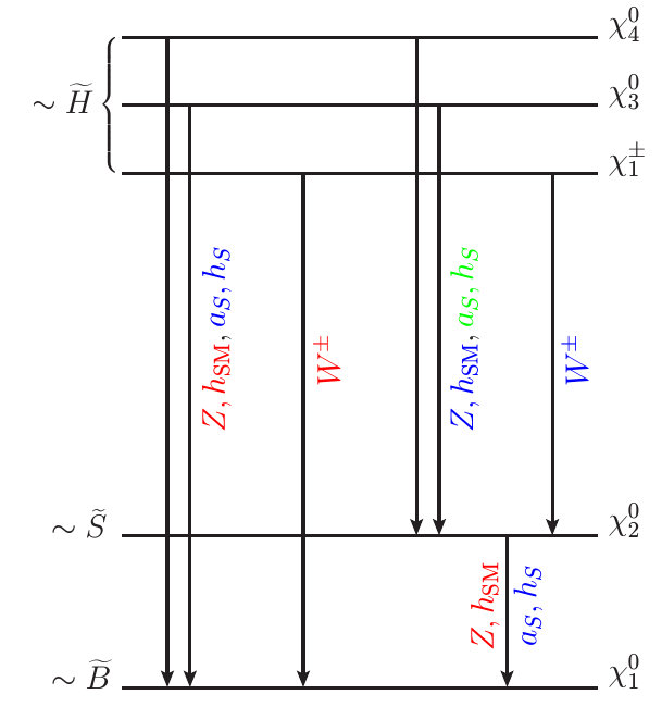


In the top panel of figure 11 we illustrate these two possible hierarchies of the neutralinos and the lighter chargino via a pair of level diagrams Potter:2015wsa; Abdallah:2019znp that also indicate for the respective scenarios the viable two-body decays of various ewinos. In the bottom panel of figure 11 a triplet of ternary scatter plots presents various two-body branching ratios of the heavier neutralinos, (left), (middle) and (right), respectively, along the three sides of the triangles and the associated magnitude of the singlino content () of the NLSP through the palette. These branching ratios are normalized over three suitably clubbed decay modes shown along the three axes of the equilateral triangles. These modes are classified as the ones containing the -boson, the scalars (Higgs bosons), the -boson and . Parameter points yielding significant three-body branching ratios for these states are not so common in our scenario and hence are ignored. Thus, a transition from red to blue stands for a higgsino-dominated NLSP turning into a singlino-dominated one. Our focus would be on the regions where either the singlet-like scalars ( and/or ) and/or appear in the neutralino cascades. These would lead to enhanced lepton and/or jet activity in the final state arising from associated production of the lighter chargino and the neutralinos which, in turn, would help evade the existing stringent lower bounds on their masses.1212 12 In addition to various pertinent constraints from low energy experiments, the same from the LHC analyses of the observed SM-like Higgs boson and the ones from various DM experiments, NMSSMTools also incorporates a simple-minded recast Ellwanger:2018zxt of an LHC trilepton analysis Sirunyan:2018ubx to constrain masses of higgsino-like, degenerate and . The scenarios we discuss in the present work have a third (or even a fourth) neutralino of a comparable mass and, in contrast to what is considered in ref. Ellwanger:2018zxt, the heavier neutralinos among them could decay to a lighter one in addition to their decays to the LSP. Furthermore, in such scenarios, even the lighter chargino could decay to the NLSP neutralino, a mode that has not been considered in ref. Ellwanger:2018zxt but could easily erode the bounds derived there. Interestingly, for our present analysis, the strongest lower bound on the masses of such relatively light higgsino-like states seem to originate from the reported upper bounds on the SD cross section and is in the ballpark of 270 GeV (see section 3.2).
The left plot in the bottom panel of figure 11 reveals that the branching ratios of are predominantly shared between final states with -boson and while the same for the final states with and are mostly restricted to the 10% level. As we graze along the horizontal axis from right to left, the gradual change in color (from red to blue) indicates increasing singlino-content in while branching to increases mostly at the cost of the same to -boson. Such a change in the composition of is induced by an increasing with respect to . This strips the higgsino components off both and the LSP thus resulting in their weakened coupling to -boson and hence a dwindling BR[]. Note that this is also accompanied by an increase in the coveted branching of to singlet scalars which could routinely reach the 50% level and might occasionally exceed even 80% as indicated by the blue scattered points in the upper half of the triangle.
The middle plot in the bottom panel of figure 11 sheds light on various branching ratios of which is always higgsino-like in our scenario unlike or , both of which can be singlino-like as well. The situation is necessarily different from the previous case since can undergo a richer set of cascades involving both and . This calls for a phenomenologically appropriate clubbing of the final states (which has to be different from the case of decay) leading to an appropriate set of observables as presented along the three axes of this ternary plot. The combined quantity referring to decays to the -boson and along with the LSP, plotted along the base axis, can be termed as the ‘canonical branching ratio’ of , given that these are the decay modes extensively studied by the LHC experiments, yielding stringent lower bounds on the masses of the ewinos. The left axis replaces the LSP by as a ‘non-canonical’ state whose further decay (see the left plot) would supply additional leptons and/or jets (possibly, including -jets) to the overall final state when compared to the ones to which the LHC studies are restricted. The right axis presents branching to states which, on top of , exclusively contain the singlet scalars. With these, obviously, cascades that follow would result in events that would fall drastically away from the signal regions considered by the LHC experiments in their dedicated hunt for ewinos which have always looked for the -boson or in the cascades.
Note that when is higgsino-like and nearly degenerate with , the only kinematically possible two-body decays that it can undergo are with a combined branching ratio equaling unity. Such a situation shows up as a small red region at the extreme right corner of the triangle. Any mass-split between and that allows the former to cascade to the latter requires the former to be higgsino-like (along with a higgsino-like ) and the latter to be singlino-like with . This is why the rest of the region shows up in a bluish color indicating a singlino-rich .
The decay branching ratios of a higgsino-like exhibits a behavior antipodal to which is also higgsino-like, i.e., the behavior of BR[] relative to BR[] is just the opposite to what it is for BR[] relative to BR[]. In other words, the pairs of dominant branching ratios (i) BR[] and BR[] and (ii) BR[] and BR[] behave in similar ways. A similar observation is made in ref. Calibbi:2014lga in a scenario with a bino-like LSP in the MSSM.
An altogether different situation may arise if is singlino-like and is heavier than the three nearly mass-degenerate higgsino-like states, and . This is when the decay might open up, and even could dominate, as shown in the rightmost plot of the bottom panel of figure 11. The blue line overlaid on the base axis clearly represents the spectra where is highly singlino-dominated (see palette) and hence are higgsino-like. An increase in (with respect to ) is signalled by a gradual change in color (from blue to red) as one goes up along the right axis indicating a growing singlino-content in (or, equivalently, an increasing higgsino admixture in the NLSP) and an accompanying increase in BR[]. Phenomenologically, however, such a possibility is not expected to have much impact given that it refers to a relatively heavy singlino-like state whose production at the LHC would be reasonably suppressed in the first place.
3.4.2 Combined canonical branching ratios of and
In view of the above discussion, one way to anticipate the relative extent of relaxation that the existing bounds on ewino masses could undergo is to take note of the extent of depletion in the combined canonical branching ratio of the neutralinos defined as
| (32) |
In addition, as pointed out in section 3.4, the reduction in the canonical branching ratio of into , as the new decay opens up, would also affect yields in various important final states. What finally would matter is how small the product of the canonical branching ratios of the neutralinos and the lighter chargino gets to be.
The lower is, the higher are the possibility and the extent of relaxation. In the left plot of figure 12 we illustrate how varies as a function of with the magnitude of associated being indicated by the palette-color. It reveals that can range between 3 (i.e., the maximum, when all three of decay only to ) and when other decay modes of these states (into lighter neutralinos and/or singlet-like scalars) become both accessible and favored. Salient features of this plot can be briefly described as follows in terms of regions with a higgsino-like or a singlino-like NLSP.


- •
For points with a higgsino-like NLSP (i.e., with roughly degenerate ), retains its defined maximum value of 3 for . This happens if for the singlino-like , BR which occurs when its decays to are kinematically prohibited as indicated by the varying color implying increasing (hence increasing ) as increases. This is since is mostly guaranteed in our scenario given the assured mass-splitting(s) between the higgsino-like states and the LSP (i.e., and GeV). This is broadly vindicated by the purple horizontal band with value of , extending over the range . This also implies that (and hence ) remains small over this range thus opening up the decays (which are coupling-wise favored when compared to the decay to a bino-like LSP) and to take over completely. These ensure a nearly vanishing contribution to . It is thus clear from this figure that in scenarios with a higgsino-like NLSP, can rarely get below the value of 2 (when there happens to be some appreciable branching of the higgsino-like neutralinos to singlet-like scalars).
- •
In scenarios with a singlino-like NLSP, , with being higgsino-like, it is seen that the maximum value of 3 is reached over the range . This happens when the splitting between and is not enough for the decay of the former to the latter to occur and hence each of and may undergo the decays with % branching ratio, while the same for the decay tends to touch 100%. At even smaller GeV, the decay gets closed even for the minimum allowed value of GeV in our scenario. Here, a maximum value of is attained when both of decay 100% of the times to . Conversely, touches its lowest value when the sum of these two contributions touches its minimum () as a result of an enhanced BR while mostly decaying to . It may be noted that an intermediate range of between and 2 does also exist for GeV.
In the right plot of figure 12 we present the variation of the canonical branching ratio of the lighter chargino, i.e., BR[], as a function of with the magnitude of the associated being indicated by the palette-color. This branching ratio is 100% when the mass-split between and is less than . Note that this always happens for a higgsino-like NLSP which has to be nearly degenerate with a chargino of similar nature. In contrast, a singlino-like NLSP with decreasing mass (increasing mass-split with the chargino) could bring down this canonical branching ratio even below 20%, as is seen in this plot.
To summarize, we find that in a scenario with higgsino-like NLSP, there may only be very limited scope to evade recent lower bounds from the LHC on the masses of such near-degenerate ewinos. For, these higgsino-like heavier neutralinos (, with being the NLSP) would mostly decay to assuming which the said bounds are derived in the very first place. Furthermore, a singlino-like is not expected to play any role in the present context. For, in the first place, its production rate would be suppressed not only due to its large singlino-content but also since it has to be reasonably massive to possess appreciable branchings in the non-canonical modes, i.e., .
In contrast, a scenario with a singlino-like NLSP with heavier higgsino-like neutralinos () would have a much healthier prospect of evading such bounds. This is since a singlino-like NLSP can get much lighter when compared to the higgsino-like states without getting into conflict with the experimental findings. This paves the way for relatively light higgsino-like with large enough production cross sections and big enough splits with the singlino-like NLSP to which they can decay to and hence could act to erode the experimental lower bounds on the ewino masses.

The partial decay widths of the heavier higgsino-like neutralinos/lighter chargino to the singlino-like NLSP also depend on the admixture of higgsinos in the latter state. This mixing depends primarily on two quantities: ‘’ and the mass-split, . In figure 13 we present how the higgsino admixture () in an otherwise singlino-dominated NLSP () varies as a simultaneous function of (along the horizontal axis) and ‘’ (in the palette). It is clearly seen that for a given , the higgsino admixture in the NLSP increases with increasing ‘’. This is also apparent from eqs. (79) and (80) where ‘’ refers to the singlino-dominated neutralino state. It can also be gleaned from this figure that the said admixture drops with increasing when ‘’ is held fixed.
3.4.3 Effect of ‘’ on combined non-canonical branching ratios of and
The weakened canonical branching ratios for and find explanations in the magnitudes of various non-canonical branching ratios for these states that include final states containing the singlino-dominated (NLSP) and the singlet scalars, and . Thus, the (combined) non-canonical branching ratios for these neutralino states, i.e., ] and the non-canonical branching ratio for the lighter chargino, BR[] become measures of to what extent the canonical decay modes of these heavier ewinos to (steadfastly assumed by the LHC experiments to be 100%) are starved that lead to the weakening of the experimental bounds on their masses.
The above-mentioned non-canonical branching ratios crucially depend on the value of ‘’. ‘’ not only drives the higgsino-singlino-Higgs boson (scalar) interaction involved in the decay , but also controls the mixing in the higgsino-singlino sector that affects the involved couplings in a crucial way. On the other hand, the -dependence of the -boson coupling to the neutralino states only appears through the latter (mixing). Further, the said mixing is a function of which is already discussed in section 3.4.2 (see figure 13). The actual forms of the dependencies of the squared effective couplings and (that enter the calculations of the partial decay widths of ) on ‘’ and are rather subtle, given that the latter also controls the available phase space for the decays. The expressions for these couplings are presented in eqs. (82) and (C), respectively, for a higgsino-singlino system.


The variations of these couplings, for () as the singlino-like (higgsino-like) state(s), with ‘’ are presented in figure 14 for various values of and for and GeV. Note that these plots are obtained using relations (82) and (C) which are derived considering only the higgsino-singlino sub-system but still referring to the actual neutralino eigenstates () they roughly correspond to while is all the way bino-like. As noted earlier, a varying alters which, in turn, affects the couplings. Note that these couplings also have implicit dependencies on ‘’ via neutralino mass eigenvalues. It happens to be that for the higgsino-singlino system under consideration and for the concerned range of ‘’, for all the cases shown in figure 14, the squared effective couplings, for a fixed , i.e., a fixed , increase with increasing ‘’. Furthermore, as can be gleaned from these plots, the sign on has a nontrivial impact.
On the other hand, the interaction among the higgsino-dominated chargino (), the singlino-dominated neutralino () and the -boson is given by eq. (87) which tells us that the same grows with increasing higgsino admixture in the otherwise singlino-dominated state. As we have already seen (see section 3.4.2; figure 13), this happens when ‘’ increases for a fixed mass-split between the singlino- and the higgsino-like states. As we will see soon, this phenomenon would directly influence the decay .
The partial widths for the decays receive contributions from both - (for the -- case) and -driven (for the -- case) interactions. However, in the interesting situation where the singlino-like NLSP () is not so heavy, ‘’ has to be on the smaller side. On the other hand, the dominant decay modes of to turn out to be the ones involving the -boson and while those with remaining subdominant.


The left and the right plots of figure 15 illustrate the variations of the key (combined) branching ratios BR[] and that of BR[], as functions of ‘’ (now, along the horizontal axis) and the mass-splits and , respectively, which are the actual measures of the available phase space for the decays in context and are roughly synonymous to when the higgsino-singlino mixing is not large. The (combined) branching ratio BR[] behaves in a way similar to BR[] thanks to the antipodal behavior of and , as pointed out earlier.
The contours of uniform colors roughly illustrate the variations of the branching ratios with ‘’ for various fixed ranges of the involved mass-splits. On the other hand, variations of colors for fixed values of ‘’, demonstrate the effect of varying mass-split, i.e., of changing phase space volume for the concerned decay process(es). The overall profiles are the results of the combined effects of these two on the respective branching ratios. These can be traced back to the profiles of the corresponding partial widths in each case which, in turn, are found to be the outcomes of nontrivial dependence of the involved interaction strengths on ‘’, as have been pointed out in the contexts of figures 13 and 14. To summarize, larger values of ‘’ lead to large non-canonical branching ratios, albeit in a subtle way.
In the next subsection, we will present a few benchmark points with relatively light higgsino-dominated neutralinos and a chargino in such a pNMSSM scenario thanks to the enhanced non-canonical decay branching ratios of these states that help evade the recent stringent lower bounds on their masses from the LHC experiments.
3.5 Benchmark scenarios
In this section, we discuss a few benchmark scenarios that satisfy all pertinent constraints from various low energy experiments, the bounds obtained from the LHC experiments on the observed Higgs sector and the experimental constraints on various DM observables like the relic abundance and the SI and the SD rates. On top of these, though generically found to be less constraining for the scenario under study, we now also take into account the constraints obtained from experiments dedicated to indirect detection of the DM, viz., the Fermi-LAT Fermi-LAT:2016uux and the AMS-02 Aguilar:2013qda; Accardo:2014lma and subsequently discussed in refs. Ibarra:2013zia; Giesen:2015ufa thanks to late time small values of thermally averaged for the DM particles . Furthermore, we take advantage of the relaxed lower bounds on the masses of higgsino-like ewinos resulting from a preliminary recast of a relevant LHC analysis Sirunyan:2018ubx as incorporated in NMSSMTools. The benchmark scenarios presented in table 3 broadly belong to the allowed set from our random scan of the parameter space. However, these scenarios possess optimized values of branching ratios for various decay modes of the ewinos. These not only help evade the experimental bounds presented in ref. Sirunyan:2018ubx under a recast (as mentioned above) for our scenario but are also expected to remain instrumental against recent diversified analyses Aaboud:2018jiw; Aaboud:2018sua; Aaboud:2018ngk; Aad:2019vnb; Sirunyan:2019iwo; Aad:2019vvf; Aad:2019vvi; Aad:2020qnn; ATLAS:2020ckz (and improved bounds thereof) when those are eventually subjected to recasts.
The benchmark scenarios presented in table 3 broadly belong to the allowed set from our random scan of the parameter space. However, these scenarios possess optimized values of branching ratios for various decay modes of the ewinos. These not only help evade the experimental bounds presented in ref. Sirunyan:2018ubx under a recast (as mentioned above) for our scenario but are also expected to remain instrumental against recent diversified analyses Aaboud:2018jiw; Aaboud:2018sua; Aaboud:2018ngk; Aad:2019vnb; Sirunyan:2019iwo; Aad:2019vvf; Aad:2019vvi; Aad:2020qnn; ATLAS:2020ckz (and improved bounds thereof) when those are eventually subjected to recasts.
| Input parameters | Singlet (pseudo)scalar funnel | -boson funnel | SM-like Higgs funnel | Coannihilation regime | |||
| BP1 | BP2 | BP3 | BP4 | BP5 | BP6 | BP7 | |
| 0.608 | 0.265 | 0.563 | 0.267 | 0.644 | 0.230 | 0.641 | |
| 0.093 | 0.030 | 0.142 | |||||
| 19.72 | 15.34 | 26.23 | 17.64 | 28.43 | 23.76 | 9.160 | |
| (TeV) | 2.739 | 4.731 | 9.476 | 3.916 | 4.703 | 8.926 | 6.407 |
| (TeV) | 8.219 | 5.653 | 7.083 | 9.961 | 9.705 | ||
| (GeV) | 46.83 | 38.42 | 42.16 | 0.423 | 2.647 | ||
| (GeV) | 381.9 | 350.8 | 381.2 | 352.3 | 396.2 | ||
| (GeV) | 37.21 | 43.14 | 169.4 | ||||
| Observables | |||||||
| (GeV) | 37.023 | 30.756 | 43.268 | 43.063 | 57.953 | 60.688 | 167.46 |
| (GeV) | 126.88 | 112.84 | 122.97 | 87.193 | 143.82 | 108.81 | 170.74 |
| (GeV) | 406.68 | 366.96 | 399.43 | 399.21 | 382.17 | 412.95 | 415.43 |
| (GeV) | 421.21 | 372.04 | 408.03 | 401.15 | 392.24 | 417.23 | 424.45 |
| (GeV) | 395.58 | 363.37 | 388.34 | 394.76 | 365.39 | 410.43 | 400.98 |
| (GeV) | 123.92 | 117.14 | 125.96 | 101.11 | 123.18 | 118.38 | 126.32 |
| (GeV) | 185.97 | 123.40 | 179.36 | 123.74 | 204.37 | 127.85 | 192.30 |
| (GeV) | 77.641 | 64.429 | 31.354 | 30.024 | 36.575 | 25.825 | 160.72 |
| , | |||||||
| , | |||||||
| , | |||||||
| , | |||||||
| , | |||||||
| 0.115 | 0.117 | 0.113 | 0.126 | 0.116 | 0.115 | 0.124 | |
| (cm2) | |||||||
| (cm2) | |||||||
| BR[] | 0.16 | 0.49 | 0.18 | 0.47 | 0.16 | 0.56 | 0.13 |
| BR[] | 0.84 | 0.51 | 0.82 | 0.53 | 0.84 | 0.44 | 0.87 |
| BR[] | 1.00 | 1.00 | 1.00 | 1.00 | 1.00 | 1.00 | 0.00 |
| BR[] | 0.00 | 0.00 | 0.00 | 0.00 | 0.00 | 0.00 | 0.91 |
| BR[] | 0.09 | 0.31 | 0.11 | 0.25 | 0.09 | 0.40 | 0.05 |
| BR[] | 0.66 | 0.41 | 0.58 | 0.22 | 0.64 | 0.31 | 0.65 |
| BR[] | 0.06 | 0.01 | 0.07 | 0.00 | 0.06 | 0.01 | 0.08 |
| BR[] | 0.14 | 0.00 | 0.18 | 0.00 | 0.12 | 0.00 | 0.14 |
| BR[] | 0.00 | 0.18 | 0.00 | 0.21 | 0.00 | 0.17 | 0.01 |
| BR[] | 0.01 | 0.09 | 0.00 | 0.31 | 0.00 | 0.11 | 0.00 |
| BR[] | 0.00 | 0.00 | 0.00 | 0.01 | 0.00 | 0.00 | 0.00 |
| BR[] | 0.04 | 0.01 | 0.06 | 0.00 | 0.09 | 0.00 | 0.08 |
| BR[] | 0.09 | 0.23 | 0.09 | 0.26 | 0.08 | 0.20 | 0.10 |
| BR[] | 0.22 | 0.15 | 0.27 | 0.34 | 0.21 | 0.16 | 0.24 |
| BR[] | 0.06 | 0.01 | 0.08 | 0.00 | 0.06 | 0.01 | 0.02 |
| BR[] | 0.57 | 0.01 | 0.54 | 0.00 | 0.62 | 0.01 | 0.61 |
| BR[] | 0.00 | 0.25 | 0.00 | 0.24 | 0.00 | 0.35 | 0.00 |
| BR[] | 0.04 | 0.33 | 0.00 | 0.16 | 0.01 | 0.26 | 0.02 |
| BR[] | 0.01 | 0.00 | 0.01 | 0.00 | 0.01 | 0.00 | 0.00 |
| BR[] | 0.01 | 0.00 | 0.01 | 0.01 | 0.01 | 0.00 | 0.00 |
| (see eq. (32)) | 0.15 (0.15) | 0.49 (0.48) | 0.18 (0.17) | 0.46 (0.50) | 0.15 (0.14) | 0.57 (0.55) | 0.13 (0.12) |
| 0.048 | 0.475 | 0.063 | 0.451 | 0.046 | 0.627 | 0.033 | |
| (fb) Ellwanger:2018zxt | 0.88 | 12.44 | 1.27 | 8.40 | 1.10 | 10.19 | 0.55 |
| (fb) Sirunyan:2018ubx; Ellwanger:2018zxt | 33.02 | 39.81 | 32.02 | 32.15 | 43.40 | 27.93 | 46.70 |
Note that even in a favorable situation with such a tailored set of branching ratios of the lighter chargino and the relevant neutralinos, it is not that straightforward to derive the relaxed lower bounds on their masses. The best one can do in the present scope is to take a conservative approach, i.e., to look out for degraded branching ratios of the neutralinos to the -boson and (in favor of decays to lighter singlet scalar(s) and/or to a lighter neutralino other than the LSP thus yielding a smaller ) and the same for the lighter chargino decaying to (in favor of ).
As far as the LHC analyses that lead to the reported mass-bounds on the ewinos are concerned, what essentially matters are the magnitudes of the production cross sections of the pertinent ewino pairs times their effective branching ratios that lead to final states of interest. Fortunately, from a previous study Abdallah:2019znp based on a rigorous CheckMATE Dercks:2016npn analysis, we are aware of their ballpark critical values in reference to an LHC analysis on final state (arising from the -mode) carried out in ref. Sirunyan:2017lae. Given that there have been steady improvements in the lower bounds on the masses of these ewinos since then (not only via the -mode but also through the -mode leading to final states with -jets, as mentioned earlier) while the concerned analyses are still to be implemented in a recast package like CheckMATE, we exercise an extra bit of caution by choosing these key branching ratios rather conservatively. It is worthwhile to note that, towards this, achieving a rather suppressed BR[] is likely to play a crucial role, besides having smaller , in relaxing the reported lower bounds on the masses of the ewinos. This is since such an arrangement renders final states with larger jet-multiplicity more frequent by depleting the ones (with multi-leptons) to which the current bounds owe the most. From the discussions in section 3.4 it has already become clear that suppression of the above key branching ratios is characteristically achieved only in scenarios with a singlino-like NLSP. Hence all the benchmark scenarios we present in table 3 have the singlino-like state as the NLSP.
Four broad classes of benchmark scenarios are presented based on the mode of annihilation of the highly bino-like DM. These include funnels involving (i) singlet (pseudo)scalar, (ii) -boson, (iii) and (iv) coannihilation with a singlino-like NLSP neutralino. Scenarios presented in each of the first three classes are further subdivided into two categories, one having and the other having as . For the coannihilation class, we present only one scenario in which .
Various relevant branching ratios of are listed for each of these benchmark scenarios. Note that BR for all the benchmark scenarios except for the last one in which DM coannihilation is in action and BR is dominant. On the other hand, the magnitudes of the individual branching ratios for the states , as shown in table 3, are checked to be pretty representative of our full set of allowed scanned data. As always has non-canonical decays for our BPs, to aid tractability at the numerical level, we downgrade the general definition of the combined (canonical) branching ratio presented earlier in section 3.4.2 (which included as well) to contain the canonical branching ratios of only, i.e., . In table 3, the branching ratios that contribute to are underlined. One can find that is on the smaller side being between for scenarios with larger (i.e., for BP1, BP3, BP5 and BP7) and are between for scenarios in which ‘’ () is somewhat smaller (i.e., for BP2, BP4 and BP6). This is since the interactions -- are found to grow with ‘’.1313 13 The forms of these interactions are derived in appendix C. Expressions of the respective decay widths are presented in ref. Choi:2004zx. This is already discussed in section 3.4.3 in reference to the left plot of figure 15.
Note that the phenomena described above already indicate a significant weakening of the canonical branching ratios of the neutralinos. On top of these, a reduced decay branching ratio BR[] (which again is seen to vary over a range similar to what mentioned above for , the reasons being very similar as well; see the right plot of figure 15) ends up in suppressing the yields in the canonical final states down to of their values assumed by the LHC experiments. Add to this the smaller production cross section (smaller by 50%–60%) of higgsino-like when compared to that of wino-like assumed by the LHC experiments. Thus, such a situation, a priori, has the potential to cause significant relaxation of the lower bounds on the masses of the ewinos as reported by the LHC analyses. Hence dedicated recast analyses are called for waadsr.
Note that BP7 representing the coannihilation regime has a (bino-like) LSP mass on a somewhat heavier ( GeV) than what is considered for all the other scenarios. The reasons are the following. Given that is a necessary requirement for finding an efficient coannihilation, all of and have competing decays to both and , accompanied by , , singlet scalars and , respectively. In addition, BR[] could now get to be significant where the photon is expected to be too soft to be detected Domingo:2018ykx. Hence the cascades of and via might lead to similar final states as when these states decay directly to the LSP. Thus, virtually, a large effective branching ratio to the LSP for these states could be envisaged. Hence stringent experimental lower bounds on their masses better not be ignored in such a situation. Note that the chosen value of ( GeV) still appears to be allowed (i.e., GeV) by the latest experimental analyses Sirunyan:2018ubx; Aad:2019vvf; Aad:2019vvi for the accompanying values of ( GeV).1414 14 Note, however, that this value of is smaller than our targeted maximum of 200 GeV (in particular, smaller than the top quark mass, though not far from it) and the restriction is predominantly of LHC origin. It may also be noted that GeV still passes some recent constraints incorporated in the package NMSSMTools. We choose to adopt a conservative line in this matter.
In the last but one row of table 3 we present, for all the benchmark points, the resultant values of cross section times the effective branching ratio, , from the processes which eventually lead to the trilepton final state, as obtained from NMSSMTools. Note that the production process would not be contributing to this trilepton final state and this can be understood from the possible decay modes of shown in table 3. These numbers are compared with the corresponding maximum values for this quantity that are allowed by the experiment Sirunyan:2018ubx and as extracted with the help of NMSSMTools following ref. Ellwanger:2018zxt. Largely, it is clear that the smaller the effective branching ratio is, the smaller is when compared to its corresponding experimental upper limit. This, in turn, demonstrates how easily such higgsino-like and with masses in the range 350 GeV– 400 GeV could have been missed by the LHC experiments when searched for in one of the most sensitive of the final states like the one with three leptons while the reported experimental lower bound on these masses from the analysis of such a final state is in the ballpark of 500 GeV Sirunyan:2018ubx. Also, the differences between the corresponding numbers in the last two rows of table 3 are indicative of a significant room for even lighter such states surviving the experimental constraints, under the circumstance.
3.6 The issue of naturalness
In this section, we briefly comment on how ‘natural’ the scenario under consideration could get to be. The well-known finetuning measure following Ellis Ellis:1986yg and Barbieri and Giudice (BG) Barbieri:1987fn is adopted which exploits the relationship between (or the weak scale) and the fundamental SUSY parameters given by
| (33) |
where are the soft masses at the weak scale for the two doublet Higgs fields, and stand for the radiative corrections to the respective masses while ‘’ is the SUSY conserving higgsino mass parameter of the MSSM. The equality tells one that unless for large cancellations (i.e., large finetuning and hence less ‘natural’), the measured value of can be obtained only if all the terms are not too different in magnitude from itself. Note that, in the first place, it has been a puzzle (known as the ‘-problem’) within the framework of the MSSM as to why a SUSY conserving parameter would at all acquire such a weak-scale value, to which the NMSSM provides a dynamical solution where . In any case, the finetuning measure itself is given by
| (34) |
where denotes the set of Lagrangian parameters that enter eq. (33).

In our analysis, the value of is obtained from NMSSMTools for each of the scanned points in the NMSSM parameter space. In figure 16 we illustrate how is distributed for the points allowed by all experimental data (as described in earlier sections) as a function of the LSP DM mass (along the horizontal axis) and the magnitude of (indicated in the palette). Note that could reach a value as low as 30 (the conventional benchmark maximum for a ‘natural’ SUSY scenario) or even lower. This is achieved notwithstanding our consideration of rather heavy top squarks and the gluino ( TeV, which are the primary spoilers of ‘naturalness’ through the terms in eq. (33) thanks to rather low values of that are found to be still viable. Nonetheless, we have checked explicitly that scenarios with top squarks and gluino as light as 2.5 TeV are seamlessly compatible with the broader physics situations we focus on in this work while being able to pull down to a value of 20 or even less thus rendering the scenarios highly natural.
4 Conclusions
A highly bino-like DM can be motivated from an ever diminishing upper bound on the DMDD cross sections. However, in the absence of comparably light sfermions and/or ewinos (as being hinted by experiments), a relatively light ( GeV) LSP DM of such a kind has to look out for annihilation funnels induced by the SM -boson, the observed SM-like Higgs boson and various other light scalars of a SUSY scenario that are yet to be ruled out experimentally. This inevitably requires the bino-like DM to have some minimal tempering with higgsinos, be it in the MSSM or in the pNMSSM, that does not spoil compliance with the DD constraints. Note that, with decoupled sfermions, the pure bino limit of a bino-dominated DM in a bino-higgsino(-singlino) system does not exist in the same sense as the pure higgsino limit for a higgsino-dominated DM in a higgsino-bino system does with its mass around 1.1 TeV.
In the MSSM, such a tempering by higgsinos could allow for an efficient enough mutual annihilation of the highly bino-like DM states (lighter than 200 GeV) only via the well-known - and -funnels (with either or ) thus ensuring compliance with the experimental upper bound on DM relic abundance. However, stringent lower bounds on that can be derived from recent direct searches for the light ewinos at the LHC might have started posing some reasonable threat to the viability of such a light bino-dominated DM candidate, especially when it annihilates via -funnel.
In this work, we have demonstrated that the flexibility and the resulting richness of the ewino and the scalar spectrum of the pNMSSM, in tandem, could mitigate the situation and allow for a relatively light (below about 200 GeV, or more particularly, even below 100 GeV), highly bino-like neutralino DM (with more than 95% bino-content). Going beyond the MSSM, on the one hand, this scenario is known to offer additional DM annihilation funnels in the form of relatively light singlet-like scalars () over a significant region of the pNMSSM parameter space thus allowing for a continuous range of the LSP mass which can have the right relic for suitable masses of , i.e., or . A minimal tempering of a pure bino LSP is nonetheless necessary. For moderate to large values of ‘’, not so heavy higgsino-like states and a singlino-like NLSP could induce such tempering which in our case is shared between the higgsinos (up to 5%) and the singlino (up to 1%).
The singlino-like NLSP plays a crucial role in the present study in at least three ways.
- •
First, in a favorable region of the pNMSSM parameter space, the singlino-like NLSP could serve as a viable coannihilating state for a highly bino-like LSP DM with mass below 200 GeV (and which is unable to funnel) thus ensuring DM abundance in the right ballpark over an extended range of the DM mass. Note that recent LHC searches for ewinos, even after their proper recast, are unlikely to allow higgsino-like such states with mass GeV. On top of that, the latest upper bounds on the SD rates are found to put a stringent restriction on ( GeV). Hence such higgsino-like states would be unable to play the role of coannihilating agents for the DM in the said mass range. The wino and the sfermions being considered to be rather heavy in this study, the singlino emerges as the only viable coannihilating state. In principle, the DM wash out process in the early Universe could receive simultaneous contributions from both a funnel-annihilation and a coannihilation process when .
- •
Second, the tempering of the DM by a light singlino-like state provides new mechanisms in moderating the -- and -- couplings in such ways that the SI and the SD rates, respectively, could be tamed to comply with their experimentally allowed values away from the well-known MSSM blind spot regimes.
In particular, in a light bino-higgsino system, for which the MSSM (gauge) coupling blind spot condition, relevant to the SI rate, could be satisfied only when there is a relative sign between and , now can have a suppressed overall -- interaction even when these latter parameters have the same sign. In such a situation, the enhanced gauge coupling contribution (, for -- interaction) to this effective interaction strength could get canceled in the bino-higgsino-singlino system by the -dependent -- interaction, for moderate to large ‘’ and .
On the other hand, the SD rate governed by the -- interaction strength () and which is suppressed in the MSSM when is small (vanishing in the limit ), could now have new compensating terms in its expression in the presence of a light singlino-like state. These can then play their roles in suppressing the relevant coupling even for larger values, again for a moderate to large value of ‘’.
- •
Finally, the presence of such a light singlino-like NLSP, when accompanied by light singlet scalars of the scenario, could significantly alter the simplistic decay patterns (as assumed by the LHC experiments) of the immediately heavier ewinos which, in our case, are higgsino-like. This is particularly true for moderate to large values of ‘’. An already degraded lower bound on the masses of such higgsino-like states, derived via recast of the relevant LHC analyses which instead assume wino-like such states but still based on the same simple decay pattern as the latter, would then be further eroded. Hence a much smaller value of than what is currently expected can still be allowed thus keeping open the feasibility of a more ‘natural’ scenario.
We demonstrated with examples how in various different scenarios such a spectrum could erode yields in the and - final states, the ones that traditionally appear as much cleaner and hence possess with high sensitivities to the LHC experiments.
It is further demonstrated that the viability of a highly bino-like neutralino DM with a mass around 100 GeV (or less) depends much upon the magnitude of and, as can be expected, the smaller we go in the mass of this DM neutralino, for a fixed value of , the larger the value of we require to keep a check on its SI scattering rates which are highly constrained from experiments. Furthermore, for the DM mass below the top quark mass, larger values of could also crucially aid DM annihilation to via the singlet-like pseudoscalar () funnel as the involved coupling strength increases with .
All these features are backed by analytical results that we obtained for the first time in the framework of a bino-higgsino-singlino system and are presented in a three-part appendix. We also observe that the phenomenology of such a scenario but with a higgsino-like NLSP almost mimics an MSSM scenario with a similar spectrum.
In conclusion, it should be stressed that recent and upcoming analyses from the LHC experiments would shed important light on the viability of such a relatively light, highly bino-like DM in the framework of pNMSSM by keeping track of the lower bound on that these could extract. Under the current circumstances, this would involve a rather dedicated recast of the relevant LHC analyses involving not only the lepton-rich final states which are traditionally known to be rather sensitive to such new physics scenarios but also the ones with the bottom quarks, the taus and the photons in the final state which arise in the cascades of the ewinos involving Higgs(-like) scalars and can occasionally be boosted as well. Nonetheless, the results obtained by us in a recent work using a limited recast and employed in this work already indicate that there is still much room left in the bottom as far as a lower bound on of the pNMSSM is concerned which can still be consistent with most other relevant constraints including those from the DM experiments and could render the scenario rather ‘natural’. However, it is the experimental constraint on the SD rate that puts the most stringent lower bound on in the current scenario.
On the other hand, we find that the future DARWIN experiment would be able to probe the entire volume of the pNMSSM parameter space of such a scenario that gives rise to a highly bino-like LSP DM by studying the DM-nucleon SD scattering even when the DM-nucleon SI scattering cross section sinks below the neutrino floor.
Results presented in this work follow from a conservative approach of not incorporating a downward scaling of the DD rates when the DM relic abundance falls below its 2 lower bound. However, when incorporated, such a scaling could open up new allowed regions of the parameter space by pulling down the DD rates below their respective upper bounds that assume the DM abundance to be equal to the central value obtained by the Planck collaboration. This, in turn, could allow for some increased level of mixings of the higgsino and the singlino states in an otherwise bino-dominated LSP DM. The analytical results presented for the first time in this work by considering a coupled system of these three ewino states would aid a better understanding of phenomena that involve these states in a nontrivial way.
Acknowledgements.
WA and SR are supported by the funding available from the Department of Atomic Energy (DAE), Government of India for the Regional Centre for Accelerator-based Particle Physics (RECAPP) at Harish-Chandra Research Institute (HRI). WA also acknowledges support from the XII Plan Neutrino Project funded by the DAE at HRI. The authors thank U. Ellwanger, C. Hugonie and T. Stefaniak for useful discussions. They acknowledge the use of the High Performance Scientific Computing facility and RECAPP’s Cluster Computing facility at HRI and would like to thank Rajeev Kumar and Ravindra Yadav for their technical help at these facilities.Appendices
Appendix A Scalar-neutralino-neutralino interactions
Neutralino-neutralino-scalar interactions are given in their general forms in ref. Ellwanger:2009dp. For the -even scalars () these are given by
| (35) | |||||
where and the ‘’ matrix diagonalizes the mass-squared matrix of eq. (6). For the -odd scalars () the corresponding expression is
| (36) | |||||
where matrix ‘’ diagonalizes the mass-squared matrix of eq. (9).
In a more convenient basis (of eq. (8)) for the -even scalars, and for the corresponding scalar states , eq. (35) reduces to
| (37) | |||||
On the other hand, for the -odd scalars, , interacting with a pair of neutralinos, and , eq. (36), in terms of diagonalization matrix of eq. (10), is given by,
| (38) | |||||
In the present study, we consider a bino-like neutralino LSP and a rather heavy wino which is effectively decoupled. Consequently, wino admixtures in the lighter neutralino states can be ignored.
Appendix B The bino-higgsino-singlino system and the SI and the SD blind spots
For a decoupled wino, the , symmetric neutralino mass-matrix of eq. (19) effectively reduces to a matrix in the basis , comprising of the bino, the higgsinos and the singlino, and is given by
| (39) |
In the absence of -violation, symmetric matrix can be diagonalized by an orthogonal matrix ‘’, i.e.,
| (40) |
Sticking all through to the conventions/assignments of eq. (19) but for dropping the wino, the neutralino mass-eigenstates are again represented by
| (41) |
with while . Expressions for the elements and the physical mass of the -neutralino () can be obtained by using
| (42) |
and exploiting the orthogonality of the matrix ‘’, i.e.,
| (43) |
This leads to the following set of equations:
| (44) | |||||
| (45) | |||||
| (46) | |||||
| (47) |
By adopting the approach of ref. ElKheishen:1992yv we divide the above four equations by (assuming ) and pick up a suitable set of three eqs. (45), (46) and (47). We thus find the following relation between the bino () and the singlino () admixtures in the -th neutralino and the similar ones for the two higgsino admixtures ( and ) to the same singlino admixture:
| (48) | |||||
| (49) | |||||
| (50) |
By using the unitarity condition (for the system)
| (51) |
expressions for the elements can be obtained, e.g.,
| (52) |
where
| (53) |
and
| (54) | |||||
Meanwhile, in the effective MSSM (decoupling) limit, i.e., and Ellwanger:2009dp (and ), one recovers the bino-higgsino system of the MSSM. Thus, the expression in eq. (54) reduces to
and this, when plugged in into eq. (52), results in . Furthermore, in this limit, from eqs. (48), (49) and (50), one can find
| (55) |
| (56) |
Eqs. (55) and (56) agree with the corresponding expressions for the bino-higgsino system of the MSSM Djouadi:2001kba; Pierce:2013rda.
To find the SI blind spot condition for the bino-higgsino-singlino system we refer to the generic -even scalar-neutralino-neutralino coupling of eq. (37) which, for a pair of LSPs (==1) and by dropping the wino-related term proportional to , reduces to
| (57) | |||||
From eq. (57) and considering that there is no mixing between the singlet and the doublet scalars () and that the mixing between the doublet Higgs states could also be ignored (i.e., and ) for large enough and Badziak:2015exr, the coupling of the SM-like Higgs boson with an LSP pair is given by
| (58) | |||||
Using eqs. (48), (49), (50) and (52), eq. (58) reduces to
| (59) |
A vanishing that results in a (coupling) blind spot for the most dominant () contribution to the SI scattering cross section of the DM (LSP) off the nucleus, as long as and , thus implies
| (60) |
For and the third term of the left-hand side of eq. (60) is suppressed compared to the second term there. This is a situation leading to at best a moderate splitting between the singlino-like NLSP and the bino-like LSP, a setup which is studied in detail in the present work. Under such a circumstance, the coupling blind spot condition can be approximated as
| (61) |
Compliance with eq. (61) under two specific situations may worth a mention. A closer inspection reveals that when and carry the same sign, such compliance requires and to have a relative sign between them which, in turn, implies . Thus, these together amount to a relative sign between and . Such a requirement is indeed vindicated by our numerical scan (see the bottom, right plot of figure 7) when compliance with experimental bound on the SI scattering cross section is demanded. If, instead, and carry a relative sign between them, the situation is a little more involved. ‘’ could take both signs depending on the absolute magnitudes and signs on and the term .
By its sheer appearance, eq. (60) turns out to be the suitable one for describing the blind spot condition for a bino-like LSP in a bino-higgsino-singlino system of neutralinos.1515 15 Note that an equivalent condition could be arrived at by using the set of eqs. (44), (45) and (46) (instead of the set (45), (46) and (47)) which will be suitable for describing the blind spot situation with a singlino-like LSP in such a system. This is clearly demonstrated when one is able to recover the coupling blind spot condition for the bino-higgsino system of the MSSM Huang:2014xua in the decoupling limit, i.e.,
| (62) |
Note that condition (62) has its sole origin in the gauge interaction of a pair of bino-dominated LSPs with the SM-like Higgs boson.
Note that while in the MSSM case of eq. (62) where the blind spot condition can only be satisfied for and carrying a relative sign between them, such a condition given by eq. (61) for the NMSSM could get satisfied for and having the same sign as well. This happens for moderate to large ‘’ and negative ‘’ (as discussed earlier). The former, in turn, tempers the bino-like LSP with some singlino admixture.
To study the blind spot in SI cross section with origin in the interference between the scattering diagrams mediated by and the heavy MSSM-like -even Higgs boson, ‘’, one needs to know the coupling of a pair of LSPs with the latter. The same is found from the general expression for such couplings as given in eq. (57) and by considering 1 and and is given by
| (63) | |||||
As before, substituting eqs. (48), (49), (50) and (52) into eq. (63), one finds
| (64) |
Now, the SI scattering cross section of the DM particle off a nucleon ‘’ (proton () or neutron (), in the nucleus of the detector material) is given by Badziak:2016qwg; Cao:2018rix
| (65) |
where is the reduced mass of the system comprising of the DM and the nucleon. The general expression for the coupling of a -even scalar with a pair of nucleons, of eq. (26), in the basis of eq. (8) is given by Badziak:2015exr
| (66) |
where is the mass of the nucleon, are the combinations of various nucleon form factors appropriate for the nucleon ‘’ as presented in ref. Belanger:2013oya; Badziak:2016qwg.
Substituting eqs. (66), (59) and (64) into eq. (65) and ignoring the contribution from the -even singlet-like Higgs (given the nucleons couple only to the minuscule doublet content within the singlet-like scalar), one finds
| (67) | |||||
where we have made the standard assumption . Since for a bino-dominated LSP and , blind spot for the SI cross section arises when the quantity within the big square bracket on the right-hand side of eq. (67) vanishes. The last term represents the contribution from the heavy -even MSSM-like Higgs boson and is suppressed by its mass. Dividing the entire content further by to cast the resulting condition into a familiar form, the latter appears as
| (68) |
As before, the corresponding blind spot condition pertaining to the bino-higgsino system of the MSSM with a bino-like LSP is retrieved from eq. (B) in the decoupling limit and is given by
| (69) |
For large when can be dropped and , the blind spot condition (69) becomes identical to the one obtained for the MSSM with a bino-like LSP Huang:2014xua; Badziak:2017the, i.e.,
| (70) |
A corresponding blind spot condition for the SD scattering cross section can be obtained for the bino-higgsino-singlino system by considering where, by using eqs. (49), (50) and (52), one can find
An MSSM-like SD blind spot condition is trivially found when whereby vanishes Cheung:2012qy. However, in the NMSSM, it is also possible to find a small SD cross section if the terms within the square bracket of eq. (B) could arrange to cancel each other. Note that the last term is always positive. The second term is positive (negative) if and have the same (opposite) signs. In the first case, the cancellation has to occur between the first term and the sum of the rest two. In the second case, which may not be too natural, the cancellation should take place between the sum of the first two and the last term. It must be noted, that neither nor could become too large compared to the mass of the bino-like LSP if an overall cancellation has to take place in the presence of the first term, i.e., . In figure 4 we encounter such a vanishing of the quantity for certain small splittings between and when both carry the same sign. This may, however, induce a critically large bino-singlino mixing in the LSP which in turn could be disfavored by the constraints on the SI rates. In any case, this is again purely an NMSSM phenomenon showcasing a tempering of the bino-dominated LSP by the singlino which necessarily has to be assisted by the higgsinos. Furthermore, in the limit (i.e., for a highly bino-like LSP), while eq. (67) leads to , eq. (B) results in Carena:2018nlf.
Another much relevant quantity in the current context is which is a measure of the total higgsino admixture in the LSP and which controls scalar (Higgs boson) couplings to a pair of bino-like LSPs. Again, using eqs. (49), (50) and (52), one finds, for the bino-higgsino-singlino system
| (72) | |||||
A little scrutiny reveals that eqs. (52), (53), (54), (B) and (72) are all symmetric under simultaneous flips in signs on each of , and . Hence the quantities , and which the above-mentioned equations describe all exhibit this symmetry. We have pointed this out in our discussions on figures 2, 3 and 4 in section 2.3.2.
Before we end this section of the appendix it is worth taking a look at how the higgsino-singlino system of the NMSSM follows from the set of relations derived for the bino-higgsino-singlino system. Towards this, dividing eqs. (44), (45), (46) and (47) by (assuming ) but this time picking up the three eqs. (44), (45) and (46) as the ones appropriate for the purpose in hand, one can find the following relations among ’s:
| (73) | |||||
| (74) | |||||
| (75) |
Using eqs. (73), (74) and (75) one can now retrieve the following set of familiar Badziak:2015exr relations for the higgsino-singlino system for decoupled (thus, ) and :
| (76) | |||
| (77) |
This reduced system would suffice for our presentation of appendix C where we discuss the -dependence of various partial widths of heavier higgsino-like neutralinos decaying to a singlino-like NLSP through the relevant ewino couplings.
Appendix C -dependence of the relevant ewino partial decay widths
Following section 3.4, it is sufficient to study the partial widths of two types of decays of heavier higgsino-like neutralinos to a singlino-like NLSP: and the same for the lighter higgsino-like chargino decaying to the NLSP: . The dependencies of these partial widths on ‘’ are of crucial importance. Again, it suffices to consider such a dependence only through the involved couplings since the same through the phase space measures (i.e., the involved mass-splits) is generally subdominant unless at the boundaries. Thus, with only higgsinos and singlino involved, it would be sufficient to restrict ourselves to a higgsino-singlino system discussed at the end of appendix B.
The decay width of a neutralino () to another neutralino () and a -boson is given by
| (78) |
By using eqs. (76), (77) and the involved unitarity condition (, for the higgsino-singlino system), individual elements on the right-hand side of eq. (78) can be expressed as
| (79) | |||||
| (80) |
along with
| (81) |
Clearly, , and are explicit functions of ‘’. These also have some implicit dependence on ‘’ via the neutralino mass, . It can be checked from eqs. (79), (80) and (81) that when implying the -th neutralino is a pure higgsino, both and equal to 1/2 while . With increasing ‘’, higgsino component in the otherwise singlino-dominated neutralino increases at the expense of the higgsino content of the higgsino-dominated state(s).
Substituting the expressions for the elements in eqs. (79) and (80) into the right-hand side of eq. (78), we find
| (82) |
For our discussion, and is taken to be higgsino(singlino)-like such that and when the terms can be ignored. In this limit, expression (82) reduces to
| (83) |
Expression (83) reveals that the coupling of such a pair of neutralinos to the -boson increases with increasing ‘’ when the participating masses could be held fixed. On the other hand, the variation of this coupling with is more subtle and depends upon relative signs among the mass parameters.
Similarly, the decay width of a neutralino () to another neutralino () and the SM-like Higgs boson is given by
| (84) |
Again, substituting the expressions for the elements in eqs. (79), (80) and (81) into the right-hand side of eq. (84), we find
Using similar approximations as has been done after eq. (82), eq. (C) simplifies to
| (86) |
Again, just like in the case of , here also one finds increases with increasing ‘’ under similar circumstances.
Finally, the partial decay width of a chargino to a lighter neutralino and a -boson would also go as the involved coupling-squared and is given by
| (87) | |||||
With a decoupled wino that we consider, the lighter chargino is higgsino-like. Thus, the wino components in the same, while the higgsino admixtures . As before, . Thus, will depend on the two higgsino components, and of the only neutralino state taking part in the interaction. Again, it is straightforward to expect from expressions (79) and (80) that this coupling also increases with ‘’ when the -th state is singlino-dominated to start with.
References
- (1) N. Arkani-Hamed, A. Delgado and G. F. Giudice, Nucl. Phys. B 741 (2006), 108-130 doi:10.1016/j.nuclphysb.2006.02.010 [arXiv:hep-ph/0601041 [hep-ph]].
- (2) A. Pierce, N. R. Shah and K. Freese, [arXiv:1309.7351 [hep-ph]].
- (3) K. Fukushima, C. Kelso, J. Kumar, P. Sandick and T. Yamamoto, Phys. Rev. D 90 (2014) no.9, 095007 doi:10.1103/PhysRevD.90.095007 [arXiv:1406.4903 [hep-ph]].
- (4) S. Baum, P. Sandick and P. Stengel, Phys. Rev. D 102 (2020) no.1, 015026 doi:10.1103/PhysRevD.102.015026 [arXiv:2004.02834 [hep-ph]].
- (5) S. Chakraborty and T. S. Roy, Phys. Rev. D 100 (2019) no.3, 035020 doi:10.1103/PhysRevD.100.035020 [arXiv:1904.10144 [hep-ph]].
- (6) J. R. Ellis, T. Falk, K. A. Olive and M. Srednicki, Astropart. Phys. 13 (2000), 181-213 [erratum: Astropart. Phys. 15 (2001), 413-414] doi:10.1016/S0927-6505(99)00104-8 [arXiv:hep-ph/9905481 [hep-ph]].
- (7) G. Aad et al. [ATLAS], Eur. Phys. J. C 80 (2020) no.2, 123 doi:10.1140/epjc/s10052-019-7594-6 [arXiv:1908.08215 [hep-ex]].
- (8) G. Aad et al. [ATLAS], Phys. Rev. D 101 (2020) no.5, 052005 doi:10.1103/PhysRevD.101.052005 [arXiv:1911.12606 [hep-ex]].
- (9) G. Aad et al. [ATLAS], Phys. Rev. D 101 (2020) no.3, 032009 doi:10.1103/PhysRevD.101.032009 [arXiv:1911.06660 [hep-ex]].
- (10) P. Huang, R. A. Roglans, D. D. Spiegel, Y. Sun and C. E. M. Wagner, Phys. Rev. D 95 (2017) no.9, 095021 doi:10.1103/PhysRevD.95.095021 [arXiv:1701.02737 [hep-ph]].
- (11) M. Badziak, M. Olechowski and P. Szczerbiak, Phys. Lett. B 770 (2017), 226-235 doi:10.1016/j.physletb.2017.04.059 [arXiv:1701.05869 [hep-ph]].
- (12) M. van Beekveld, W. Beenakker, S. Caron and R. Ruiz de Austri, JHEP 04 (2016), 154 doi:10.1007/JHEP04(2016)154 [arXiv:1602.00590 [hep-ph]].
- (13) M. Abdughani, L. Wu and J. M. Yang, Eur. Phys. J. C 78 (2018) no.1, 4 doi:10.1140/epjc/s10052-017-5485-2 [arXiv:1705.09164 [hep-ph]].
- (14) J. L. Feng, K. T. Matchev and F. Wilczek, Phys. Lett. B 482 (2000), 388-399 doi:10.1016/S0370-2693(00)00512-8 [arXiv:hep-ph/0004043 [hep-ph]].
- (15) H. Baer, A. Mustafayev, S. Profumo, A. Belyaev and X. Tata, JHEP 07 (2005), 065 doi:10.1088/1126-6708/2005/07/065 [arXiv:hep-ph/0504001 [hep-ph]].
- (16) A. Masiero, S. Profumo and P. Ullio, Nucl. Phys. B 712 (2005), 86-114 doi:10.1016/j.nuclphysb.2005.01.028 [arXiv:hep-ph/0412058 [hep-ph]].
- (17) H. Baer, A. Mustafayev, E. K. Park and S. Profumo, JHEP 07 (2005), 046 doi:10.1088/1126-6708/2005/07/046 [arXiv:hep-ph/0505227 [hep-ph]].
- (18) H. Baer, T. Krupovnickas, A. Mustafayev, E. K. Park, S. Profumo and X. Tata, JHEP 12 (2005), 011 doi:10.1088/1126-6708/2005/12/011 [arXiv:hep-ph/0511034 [hep-ph]].
- (19) A. Birkedal-Hansen and B. D. Nelson, Phys. Rev. D 64 (2001), 015008 doi:10.1103/PhysRevD.64.015008 [arXiv:hep-ph/0102075 [hep-ph]].
- (20) A. Birkedal-Hansen and B. D. Nelson, Phys. Rev. D 67 (2003), 095006 doi:10.1103/PhysRevD.67.095006 [arXiv:hep-ph/0211071 [hep-ph]].
- (21) P. A. R. Ade et al. [Planck], Astron. Astrophys. 594 (2016), A13 doi:10.1051/0004-6361/201525830 [arXiv:1502.01589 [astro-ph.CO]].
- (22) N. Aghanim et al. [Planck], Astron. Astrophys. 641 (2020), A6 doi:10.1051/0004-6361/201833910 [arXiv:1807.06209 [astro-ph.CO]].
- (23) E. Aprile et al. [XENON], Phys. Rev. Lett. 121 (2018) no.11, 111302 doi:10.1103/PhysRevLett.121.111302 [arXiv:1805.12562 [astro-ph.CO]].
- (24) E. Aprile et al. [XENON], Phys. Rev. Lett. 122 (2019) no.14, 141301 doi:10.1103/PhysRevLett.122.141301 [arXiv:1902.03234 [astro-ph.CO]].
- (25) C. Amole et al. [PICO], Phys. Rev. D 100 (2019) no.2, 022001 doi:10.1103/PhysRevD.100.022001 [arXiv:1902.04031 [astro-ph.CO]].
- (26) M. Ackermann et al. [Fermi-LAT], Astrophys. J. 840 (2017) no.1, 43 doi:10.3847/1538-4357/aa6cab [arXiv:1704.03910 [astro-ph.HE]].
- (27) A. Albert et al. [Fermi-LAT and DES], Astrophys. J. 834 (2017) no.2, 110 doi:10.3847/1538-4357/834/2/110 [arXiv:1611.03184 [astro-ph.HE]].
- (28) P. Agrawal, B. Batell, P. J. Fox and R. Harnik, JCAP 05 (2015), 011 doi:10.1088/1475-7516/2015/05/011 [arXiv:1411.2592 [hep-ph]].
- (29) K. Freese, A. Lopez, N. R. Shah and B. Shakya, JHEP 04 (2016), 059 doi:10.1007/JHEP04(2016)059 [arXiv:1509.05076 [hep-ph]].
- (30) A. Butter, S. Murgia, T. Plehn and T. M. P. Tait, Phys. Rev. D 96 (2017) no.3, 035036 doi:10.1103/PhysRevD.96.035036 [arXiv:1612.07115 [hep-ph]].
- (31) A. Achterberg, M. van Beekveld, S. Caron, G. A. Gómez-Vargas, L. Hendriks and R. Ruiz de Austri, JCAP 12 (2017), 040 doi:10.1088/1475-7516/2017/12/040 [arXiv:1709.10429 [hep-ph]].
- (32) M. Aaboud et al. [ATLAS], JHEP 01 (2018), 055 doi:10.1007/JHEP01(2018)055 [arXiv:1709.07242 [hep-ex]].
- (33) A. M. Sirunyan et al. [CMS], JHEP 09 (2018), 007 doi:10.1007/JHEP09(2018)007 [arXiv:1803.06553 [hep-ex]].
- (34) E. Bagnaschi, H. Bahl, E. Fuchs, T. Hahn, S. Heinemeyer, S. Liebler, S. Patel, P. Slavich, T. Stefaniak and C. E. M. Wagner, et al. Eur. Phys. J. C 79 (2019) no.7, 617 doi:10.1140/epjc/s10052-019-7114-8 [arXiv:1808.07542 [hep-ph]].
- (35) G. Aad et al. [ATLAS], Phys. Rev. Lett. 125 (2020) no.5, 051801 doi:10.1103/PhysRevLett.125.051801 [arXiv:2002.12223 [hep-ex]].
- (36) M. Carena, J. Osborne, N. R. Shah and C. E. M. Wagner, Phys. Rev. D 98 (2018) no.11, 115010 doi:10.1103/PhysRevD.98.115010 [arXiv:1809.11082 [hep-ph]].
- (37) M. Aaboud et al. [ATLAS], Phys. Rev. D 97 (2018) no.5, 052010 doi:10.1103/PhysRevD.97.052010 [arXiv:1712.08119 [hep-ex]].
- (38) L. Calibbi, J. M. Lindert, T. Ota and Y. Takanishi, JHEP 11 (2014), 106 doi:10.1007/JHEP11(2014)106 [arXiv:1410.5730 [hep-ph]].
- (39) U. Ellwanger, C. Hugonie and A. M. Teixeira, Phys. Rept. 496 (2010), 1-77 doi:10.1016/j.physrep.2010.07.001 [arXiv:0910.1785 [hep-ph]].
- (40) J. E. Kim and H. P. Nilles, Phys. Lett. B 138 (1984), 150-154 doi:10.1016/0370-2693(84)91890-2
- (41) C. Beskidt, W. de Boer, D. I. Kazakov and S. Wayand, Phys. Lett. B 771 (2017), 611-618 doi:10.1016/j.physletb.2017.06.016 [arXiv:1703.01255 [hep-ph]].
- (42) G. Belanger, F. Boudjema, C. Hugonie, A. Pukhov and A. Semenov, JCAP 09 (2005), 001 doi:10.1088/1475-7516/2005/09/001 [arXiv:hep-ph/0505142 [hep-ph]].
- (43) J. F. Gunion, D. Hooper and B. McElrath, Phys. Rev. D 73 (2006), 015011 doi:10.1103/PhysRevD.73.015011 [arXiv:hep-ph/0509024 [hep-ph]].
- (44) D. Das and U. Ellwanger, JHEP 09 (2010), 085 doi:10.1007/JHEP09(2010)085 [arXiv:1007.1151 [hep-ph]].
- (45) D. Albornoz Vasquez, G. Belanger, C. Boehm, A. Pukhov and J. Silk, Phys. Rev. D 82 (2010), 115027 doi:10.1103/PhysRevD.82.115027 [arXiv:1009.4380 [hep-ph]].
- (46) D. T. Cumberbatch, D. E. Lopez-Fogliani, L. Roszkowski, R. Ruiz de Austri and Y. L. S. Tsai, [arXiv:1107.1604 [astro-ph.CO]].
- (47) T. Han, Z. Liu and S. Su, JHEP 08 (2014), 093 doi:10.1007/JHEP08(2014)093 [arXiv:1406.1181 [hep-ph]].
- (48) C. Cheung, M. Papucci, D. Sanford, N. R. Shah and K. M. Zurek, Phys. Rev. D 90 (2014) no.7, 075011 doi:10.1103/PhysRevD.90.075011 [arXiv:1406.6372 [hep-ph]].
- (49) J. Guo, J. Li, T. Li and A. G. Williams, Phys. Rev. D 91 (2015) no.9, 095003 doi:10.1103/PhysRevD.91.095003 [arXiv:1409.7864 [hep-ph]].
- (50) T. Gherghetta, B. von Harling, A. D. Medina, M. A. Schmidt and T. Trott, Phys. Rev. D 91 (2015), 105004 doi:10.1103/PhysRevD.91.105004 [arXiv:1502.07173 [hep-ph]].
- (51) X. J. Bi, L. Bian, W. Huang, J. Shu and P. F. Yin, Phys. Rev. D 92 (2015), 023507 doi:10.1103/PhysRevD.92.023507 [arXiv:1503.03749 [hep-ph]].
- (52) J. Cao, L. Shang, P. Wu, J. M. Yang and Y. Zhang, JHEP 10 (2015), 030 doi:10.1007/JHEP10(2015)030 [arXiv:1506.06471 [hep-ph]].
- (53) L. Shang, Y. He, J. Lian and Y. Pan, Eur. Phys. J. C 78 (2018) no.5, 390 doi:10.1140/epjc/s10052-018-5827-8 [arXiv:1804.08797 [hep-ph]].
- (54) R. Dermisek and J. F. Gunion, Phys. Rev. Lett. 95 (2005), 041801 doi:10.1103/PhysRevLett.95.041801 [arXiv:hep-ph/0502105 [hep-ph]].
- (55) N. D. Christensen, T. Han, Z. Liu and S. Su, JHEP 08 (2013), 019 doi:10.1007/JHEP08(2013)019 [arXiv:1303.2113 [hep-ph]].
- (56) D. G. Cerdeño, P. Ghosh, C. B. Park and M. Peiró, JHEP 02 (2014), 048 doi:10.1007/JHEP02(2014)048 [arXiv:1307.7601 [hep-ph]].
- (57) J. Cao, F. Ding, C. Han, J. M. Yang and J. Zhu, JHEP 11 (2013), 018 doi:10.1007/JHEP11(2013)018 [arXiv:1309.4939 [hep-ph]].
- (58) S. F. King, M. Mühlleitner, R. Nevzorov and K. Walz, Phys. Rev. D 90 (2014) no.9, 095014 doi:10.1103/PhysRevD.90.095014 [arXiv:1408.1120 [hep-ph]].
- (59) B. Dutta, Y. Gao and B. Shakya, Phys. Rev. D 91 (2015) no.3, 035016 doi:10.1103/PhysRevD.91.035016 [arXiv:1412.2774 [hep-ph]].
- (60) N. E. Bomark, S. Moretti and L. Roszkowski, J. Phys. G 43 (2016) no.10, 105003 doi:10.1088/0954-3899/43/10/105003 [arXiv:1503.04228 [hep-ph]].
- (61) U. Ellwanger and M. Rodriguez-Vazquez, JHEP 02 (2016), 096 doi:10.1007/JHEP02(2016)096 [arXiv:1512.04281 [hep-ph]].
- (62) E. Conte, B. Fuks, J. Guo, J. Li and A. G. Williams, JHEP 05 (2016), 100 doi:10.1007/JHEP05(2016)100 [arXiv:1604.05394 [hep-ph]].
- (63) M. Guchait and J. Kumar, Phys. Rev. D 95 (2017) no.3, 035036 doi:10.1103/PhysRevD.95.035036 [arXiv:1608.05693 [hep-ph]].
- (64) S. Baum, K. Freese, N. R. Shah and B. Shakya, Phys. Rev. D 95 (2017) no.11, 115036 doi:10.1103/PhysRevD.95.115036 [arXiv:1703.07800 [hep-ph]].
- (65) M. Guchait, A. H. Vijay and J. Kumar, JHEP 08 (2017), 122 doi:10.1007/JHEP08(2017)122 [arXiv:1705.06275 [hep-ph]].
- (66) U. Ellwanger and M. Rodriguez-Vazquez, JHEP 11 (2017), 008 doi:10.1007/JHEP11(2017)008 [arXiv:1707.08522 [hep-ph]].
- (67) S. Baum, N. R. Shah and K. Freese, JHEP 04 (2019), 011 doi:10.1007/JHEP04(2019)011 [arXiv:1901.02332 [hep-ph]].
- (68) D. Barducci, K. Mimasu, J. M. No, C. Vernieri and J. Zurita, JHEP 02 (2020), 002 doi:10.1007/JHEP02(2020)002 [arXiv:1910.08574 [hep-ph]].
- (69) M. Guchait and A. Roy, Phys. Rev. D 102 (2020) no.7, 075023 doi:10.1103/PhysRevD.102.075023 [arXiv:2005.05190 [hep-ph]].
- (70) M. Aaboud et al. [ATLAS], JHEP 06 (2018), 166 doi:10.1007/JHEP06(2018)166 [arXiv:1802.03388 [hep-ex]].
- (71) M. Aaboud et al. [ATLAS], Phys. Lett. B 782 (2018), 750-767 doi:10.1016/j.physletb.2018.06.011 [arXiv:1803.11145 [hep-ex]].
- (72) M. Aaboud et al. [ATLAS], JHEP 10 (2018), 031 doi:10.1007/JHEP10(2018)031 [arXiv:1806.07355 [hep-ex]].
- (73) M. Aaboud et al. [ATLAS], Phys. Lett. B 790 (2019), 1-21 doi:10.1016/j.physletb.2018.10.073 [arXiv:1807.00539 [hep-ex]].
- (74) G. Aad et al. [ATLAS], [arXiv:2005.12236 [hep-ex]].
- (75) A. M. Sirunyan et al. [CMS], JHEP 11 (2018), 018 doi:10.1007/JHEP11(2018)018 [arXiv:1805.04865 [hep-ex]].
- (76) A. M. Sirunyan et al. [CMS], Phys. Lett. B 795 (2019), 398-423 doi:10.1016/j.physletb.2019.06.021 [arXiv:1812.06359 [hep-ex]].
- (77) A. M. Sirunyan et al. [CMS], JHEP 08 (2020), 139 doi:10.1007/JHEP08(2020)139 [arXiv:2005.08694 [hep-ex]].
- (78) S. Baum, M. Carena, N. R. Shah and C. E. M. Wagner, JHEP 04 (2018), 069 doi:10.1007/JHEP04(2018)069 [arXiv:1712.09873 [hep-ph]].
- (79) J. Cao, Y. He, L. Shang, Y. Zhang and P. Zhu, Phys. Rev. D 99 (2019) no.7, 075020 doi:10.1103/PhysRevD.99.075020 [arXiv:1810.09143 [hep-ph]].
- (80) F. Domingo, J. S. Kim, V. M. Lozano, P. Martin-Ramiro and R. Ruiz de Austri, Phys. Rev. D 101 (2020) no.7, 075010 doi:10.1103/PhysRevD.101.075010 [arXiv:1812.05186 [hep-ph]].
- (81) M. Carena, H. E. Haber, I. Low, N. R. Shah and C. E. M. Wagner, Phys. Rev. D 93 (2016) no.3, 035013 doi:10.1103/PhysRevD.93.035013 [arXiv:1510.09137 [hep-ph]].
- (82) S. Baum, M. Carena, N. R. Shah, C. E. M. Wagner and Y. Wang, [arXiv:2009.10743 [hep-ph]].
- (83) J. R. Ellis, K. Enqvist, D. V. Nanopoulos and F. Zwirner, Mod. Phys. Lett. A 1 (1986), 57 doi:10.1142/S0217732386000105
- (84) R. Barbieri and G. F. Giudice, Nucl. Phys. B 306 (1988), 63-76 doi:10.1016/0550-3213(88)90171-X
- (85) H. Baer, V. Barger, P. Huang, A. Mustafayev and X. Tata, Phys. Rev. Lett. 109 (2012), 161802 doi:10.1103/PhysRevLett.109.161802 [arXiv:1207.3343 [hep-ph]].
- (86) H. Baer, V. Barger, P. Huang, D. Mickelson, A. Mustafayev and X. Tata, [arXiv:1306.2926 [hep-ph]].
- (87) A. Mustafayev and X. Tata, Indian J. Phys. 88 (2014), 991-1004 doi:10.1007/s12648-014-0504-8 [arXiv:1404.1386 [hep-ph]].
- (88) H. Baer, V. Barger and M. Savoy, Phys. Rev. D 93 (2016) no.3, 035016 doi:10.1103/PhysRevD.93.035016 [arXiv:1509.02929 [hep-ph]].
- (89) K. S. Jeong, Y. Shoji and M. Yamaguchi, JHEP 11 (2014), 148 doi:10.1007/JHEP11(2014)148 [arXiv:1407.0955 [hep-ph]].
- (90) A. Arbey, M. Battaglia and F. Mahmoudi, Eur. Phys. J. C 72 (2012), 2169 doi:10.1140/epjc/s10052-012-2169-9 [arXiv:1205.2557 [hep-ph]].
- (91) A. M. Sirunyan et al. [CMS], JHEP 03 (2018), 160 doi:10.1007/JHEP03(2018)160 [arXiv:1801.03957 [hep-ex]].
- (92) G. Aad et al. [ATLAS], Eur. Phys. J. C 80 (2020) no.8, 691 doi:10.1140/epjc/s10052-020-8050-3 [arXiv:1909.09226 [hep-ex]].
- (93) A. M. Sirunyan et al. [CMS], JHEP 03 (2018), 166 doi:10.1007/JHEP03(2018)166 [arXiv:1709.05406 [hep-ex]].
- (94) M. Aaboud et al. [ATLAS], Eur. Phys. J. C 78 (2018) no.12, 995 doi:10.1140/epjc/s10052-018-6423-7 [arXiv:1803.02762 [hep-ex]].
- (95) M. Aaboud et al. [ATLAS], Phys. Rev. D 98 (2018) no.9, 092012 doi:10.1103/PhysRevD.98.092012 [arXiv:1806.02293 [hep-ex]].
- (96) M. Aaboud et al. [ATLAS], Phys. Rev. D 100 (2019) no.1, 012006 doi:10.1103/PhysRevD.100.012006 [arXiv:1812.09432 [hep-ex]].
- (97) A. M. Sirunyan et al. [CMS], JHEP 11 (2019), 109 doi:10.1007/JHEP11(2019)109 [arXiv:1908.08500 [hep-ex]].
- (98) G. Aad et al. [ATLAS], Phys. Rev. D 101 (2020) no.7, 072001 doi:10.1103/PhysRevD.101.072001 [arXiv:1912.08479 [hep-ex]].
- (99) G. Aad et al. [ATLAS], JHEP 10 (2020), 005 doi:10.1007/JHEP10(2020)005 [arXiv:2004.10894 [hep-ex]].
- (100) [ATLAS], ATLAS-CONF-2020-015.
- (101) M. Chakraborti, U. Chattopadhyay, A. Choudhury, A. Datta and S. Poddar, JHEP 07 (2014), 019 doi:10.1007/JHEP07(2014)019 [arXiv:1404.4841 [hep-ph]].
- (102) M. Chakraborti, U. Chattopadhyay, A. Choudhury, A. Datta and S. Poddar, JHEP 11 (2015), 050 doi:10.1007/JHEP11(2015)050 [arXiv:1507.01395 [hep-ph]].
- (103) P. Athron et al. [GAMBIT], Eur. Phys. J. C 79 (2019) no.5, 395 doi:10.1140/epjc/s10052-019-6837-x [arXiv:1809.02097 [hep-ph]].
- (104) A. Datta and N. Ganguly, JHEP 01 (2019), 103 doi:10.1007/JHEP01(2019)103 [arXiv:1809.05129 [hep-ph]].
- (105) U. Ellwanger and C. Hugonie, Eur. Phys. J. C 78 (2018) no.9, 735 doi:10.1140/epjc/s10052-018-6204-3 [arXiv:1806.09478 [hep-ph]].
- (106) W. Abdallah, A. Chatterjee and A. Datta, JHEP 09 (2019), 095 doi:10.1007/JHEP09(2019)095 [arXiv:1907.06270 [hep-ph]].
- (107) D. J. Miller, R. Nevzorov and P. M. Zerwas, Nucl. Phys. B 681 (2004), 3-30 doi:10.1016/j.nuclphysb.2003.12.021 [arXiv:hep-ph/0304049 [hep-ph]].
- (108) M. Badziak, M. Olechowski and P. Szczerbiak, JHEP 03 (2016), 179 doi:10.1007/JHEP03(2016)179 [arXiv:1512.02472 [hep-ph]].
- (109) U. Ellwanger, Eur. Phys. J. C 71 (2011), 1782 doi:10.1140/epjc/s10052-011-1782-3 [arXiv:1108.0157 [hep-ph]].
- (110) H. E. Haber, R. Hempfling and A. H. Hoang, Z. Phys. C 75 (1997), 539-554 doi:10.1007/s002880050498 [arXiv:hep-ph/9609331 [hep-ph]].
- (111) A. Djouadi, Phys. Rept. 459 (2008), 1-241 doi:10.1016/j.physrep.2007.10.005 [arXiv:hep-ph/0503173 [hep-ph]].
- (112) G. Pozzo and Y. Zhang, Phys. Lett. B 789 (2019), 582-591 doi:10.1016/j.physletb.2018.12.062 [arXiv:1807.01476 [hep-ph]].
- (113) R. Kumar Barman, G. Belanger and R. M. Godbole, [arXiv:2010.11674 [hep-ph]].
- (114) D. Das, U. Ellwanger and A. M. Teixeira, JHEP 04 (2012), 067 doi:10.1007/JHEP04(2012)067 [arXiv:1202.5244 [hep-ph]].
- (115) U. Ellwanger, J. F. Gunion and C. Hugonie, JHEP 02 (2005), 066 doi:10.1088/1126-6708/2005/02/066 [arXiv:hep-ph/0406215 [hep-ph]].
- (116) U. Ellwanger and C. Hugonie, Comput. Phys. Commun. 175 (2006), 290-303 doi:10.1016/j.cpc.2006.04.004 [arXiv:hep-ph/0508022 [hep-ph]].
- (117) D. Das, U. Ellwanger and A. M. Teixeira, Comput. Phys. Commun. 183 (2012), 774-779 doi:10.1016/j.cpc.2011.11.021 [arXiv:1106.5633 [hep-ph]].
- (118) C. Cheung, L. J. Hall, D. Pinner and J. T. Ruderman, JHEP 05 (2013), 100 doi:10.1007/JHEP05(2013)100 [arXiv:1211.4873 [hep-ph]].
- (119) M. Badziak, M. Olechowski and P. Szczerbiak, PoS PLANCK2015 (2015), 130 [arXiv:1601.00768 [hep-ph]].
- (120) M. Badziak, M. Olechowski and P. Szczerbiak, JHEP 07 (2017), 050 doi:10.1007/JHEP07(2017)050 [arXiv:1705.00227 [hep-ph]].
- (121) P. Bechtle, O. Brein, S. Heinemeyer, G. Weiglein and K. E. Williams, Comput. Phys. Commun. 181 (2010), 138-167 doi:10.1016/j.cpc.2009.09.003 [arXiv:0811.4169 [hep-ph]].
- (122) P. Bechtle, O. Brein, S. Heinemeyer, O. Stål, T. Stefaniak, G. Weiglein and K. E. Williams, Eur. Phys. J. C 74 (2014) no.3, 2693 doi:10.1140/epjc/s10052-013-2693-2 [arXiv:1311.0055 [hep-ph]].
- (123) P. Bechtle, D. Dercks, S. Heinemeyer, T. Klingl, T. Stefaniak, G. Weiglein and J. Wittbrodt, [arXiv:2006.06007 [hep-ph]].
- (124) P. Bechtle, S. Heinemeyer, O. Stål, T. Stefaniak and G. Weiglein, Eur. Phys. J. C 74 (2014) no.2, 2711 doi:10.1140/epjc/s10052-013-2711-4 [arXiv:1305.1933 [hep-ph]].
- (125) P. Bechtle, S. Heinemeyer, O. Stål, T. Stefaniak and G. Weiglein, JHEP 11 (2014), 039 doi:10.1007/JHEP11(2014)039 [arXiv:1403.1582 [hep-ph]].
- (126) G. Belanger, F. Boudjema, A. Pukhov and A. Semenov, Comput. Phys. Commun. 176 (2007), 367-382 doi:10.1016/j.cpc.2006.11.008 [arXiv:hep-ph/0607059 [hep-ph]].
- (127) G. Belanger, F. Boudjema, A. Pukhov and A. Semenov, Comput. Phys. Commun. 180 (2009), 747-767 doi:10.1016/j.cpc.2008.11.019 [arXiv:0803.2360 [hep-ph]].
- (128) D. Barducci, G. Belanger, J. Bernon, F. Boudjema, J. Da Silva, S. Kraml, U. Laa and A. Pukhov, Comput. Phys. Commun. 222 (2018), 327-338 doi:10.1016/j.cpc.2017.08.028 [arXiv:1606.03834 [hep-ph]].
- (129) V. Maurer, Comput. Phys. Commun. 198 (2016), 195-215 doi:10.1016/j.cpc.2015.08.032 [arXiv:1503.01073 [cs.MS]].
- (130) M. Freytsis and Z. Ligeti, Phys. Rev. D 83 (2011), 115009 doi:10.1103/PhysRevD.83.115009 [arXiv:1012.5317 [hep-ph]].
- (131) C. Boehm, M. J. Dolan, C. McCabe, M. Spannowsky and C. J. Wallace, JCAP 05 (2014), 009 doi:10.1088/1475-7516/2014/05/009 [arXiv:1401.6458 [hep-ph]].
- (132) J. Kumar and D. Marfatia, Phys. Rev. D 88 (2013) no.1, 014035 doi:10.1103/PhysRevD.88.014035 [arXiv:1305.1611 [hep-ph]].
- (133) M. Escudero, A. Berlin, D. Hooper and M. X. Lin, JCAP 12 (2016), 029 doi:10.1088/1475-7516/2016/12/029 [arXiv:1609.09079 [hep-ph]].
- (134) G. Belanger, F. Boudjema, A. Pukhov and A. Semenov, Comput. Phys. Commun. 185 (2014), 960-985 doi:10.1016/j.cpc.2013.10.016 [arXiv:1305.0237 [hep-ph]].
- (135) P. Huang and C. E. M. Wagner, Phys. Rev. D 90 (2014) no.1, 015018 doi:10.1103/PhysRevD.90.015018 [arXiv:1404.0392 [hep-ph]].
- (136) J. Billard, L. Strigari and E. Figueroa-Feliciano, Phys. Rev. D 89 (2014) no.2, 023524 doi:10.1103/PhysRevD.89.023524 [arXiv:1307.5458 [hep-ph]].
- (137) J. L. Feng, S. Ritz, J. J. Beatty, J. Buckley, D. F. Cowen, P. Cushman, S. Dodelson, C. Galbiati, K. Honscheid and D. Hooper, et al. [arXiv:1401.6085 [hep-ex]].
- (138) D. R. Tovey, R. J. Gaitskell, P. Gondolo, Y. A. Ramachers and L. Roszkowski, Phys. Lett. B 488 (2000), 17-26 doi:10.1016/S0370-2693(00)00846-7 [arXiv:hep-ph/0005041 [hep-ph]].
- (139) C. E. Aalseth, P. Agnes, A. Alton, K. Arisaka, D. M. Asner, H. O. Back, B. Baldin, K. Biery, G. Bonfini and M. Bossa, et al. Adv. High Energy Phys. 2015 (2015), 541362 doi:10.1155/2015/541362
- (140) D. S. Akerib et al. [LUX-ZEPLIN], Phys. Rev. D 101 (2020) no.5, 052002 doi:10.1103/PhysRevD.101.052002 [arXiv:1802.06039 [astro-ph.IM]].
- (141) E. Aprile et al. [XENON], JCAP 04 (2016), 027 doi:10.1088/1475-7516/2016/04/027 [arXiv:1512.07501 [physics.ins-det]].
- (142) E. Aprile et al. [XENON], [arXiv:2007.08796 [physics.ins-det]].
- (143) U. Ellwanger and C. Hugonie, private communication.
- (144) J. Aalbers et al. [DARWIN], JCAP 11 (2016), 017 doi:10.1088/1475-7516/2016/11/017 [arXiv:1606.07001 [astro-ph.IM]].
- (145) S. F. King, M. Muhlleitner and R. Nevzorov, Nucl. Phys. B 860 (2012), 207-244 doi:10.1016/j.nuclphysb.2012.02.010 [arXiv:1201.2671 [hep-ph]].
- (146) S. F. King, M. Mühlleitner, R. Nevzorov and K. Walz, Nucl. Phys. B 870 (2013), 323-352 doi:10.1016/j.nuclphysb.2013.01.020 [arXiv:1211.5074 [hep-ph]].
- (147) J. Beuria, A. Chatterjee, A. Datta and S. K. Rai, JHEP 09 (2015), 073 doi:10.1007/JHEP09(2015)073 [arXiv:1505.00604 [hep-ph]].
- (148) J. Beuria, A. Chatterjee and A. Datta, JHEP 08 (2016), 004 doi:10.1007/JHEP08(2016)004 [arXiv:1603.08463 [hep-ph]].
- (149) C. T. Potter, Eur. Phys. J. C 76 (2016) no.1, 44 doi:10.1140/epjc/s10052-015-3867-x [arXiv:1505.05554 [hep-ph]].
- (150) M. Aguilar et al. [AMS], Phys. Rev. Lett. 110 (2013), 141102 doi:10.1103/PhysRevLett.110.141102
- (151) L. Accardo et al. [AMS], Phys. Rev. Lett. 113 (2014), 121101 doi:10.1103/PhysRevLett.113.121101
- (152) A. Ibarra, A. S. Lamperstorfer and J. Silk, Phys. Rev. D 89 (2014) no.6, 063539 doi:10.1103/PhysRevD.89.063539 [arXiv:1309.2570 [hep-ph]].
- (153) G. Giesen, M. Boudaud, Y. Génolini, V. Poulin, M. Cirelli, P. Salati and P. D. Serpico, JCAP 09 (2015), 023 doi:10.1088/1475-7516/2015/9/023 [arXiv:1504.04276 [astro-ph.HE]].
- (154) D. Dercks, N. Desai, J. S. Kim, K. Rolbiecki, J. Tattersall and T. Weber, Comput. Phys. Commun. 221 (2017), 383-418 doi:10.1016/j.cpc.2017.08.021 [arXiv:1611.09856 [hep-ph]].
- (155) S. Y. Choi, D. J. Miller and P. M. Zerwas, Nucl. Phys. B 711 (2005), 83-111 doi:10.1016/j.nuclphysb.2005.01.006 [arXiv:hep-ph/0407209 [hep-ph]].
- (156) W. Abdallah, A. Datta and S. Roy, work in progress.
- (157) M. M. El Kheishen, A. A. Aboshousha and A. A. Shafik, Phys. Rev. D 45 (1992), 4345-4348 doi:10.1103/PhysRevD.45.4345
- (158) A. Djouadi, M. Drees, P. Fileviez Perez and M. Muhlleitner, Phys. Rev. D 65 (2002), 075016 doi:10.1103/PhysRevD.65.075016 [arXiv:hep-ph/0109283 [hep-ph]].