Sphenix: Smoothed Particle Hydrodynamics for the next generation of galaxy formation simulations
Abstract
Smoothed Particle Hydrodynamics (SPH) is a ubiquitous numerical method for solving the fluid equations, and is prized for its conservation properties, natural adaptivity, and simplicity. We introduce the Sphenix SPH scheme, which was designed with three key goals in mind: to work well with sub-grid physics modules that inject energy, be highly computationally efficient (both in terms of compute and memory), and to be Lagrangian. Sphenix uses a Density-Energy equation of motion, along with variable artificial viscosity and conduction, including limiters designed to work with common sub-grid models of galaxy formation. In particular, we present and test a novel limiter that prevents conduction across shocks, preventing spurious radiative losses in feedback events. Sphenix is shown to solve many difficult test problems for traditional SPH, including fluid mixing and vorticity conservation, and it is shown to produce convergent behaviour in all tests where this is appropriate. Crucially, we use the same parameters within Sphenix for the various switches throughout, to demonstrate the performance of the scheme as it would be used in production simulations. Sphenix is the new default scheme in the Swift cosmological simulation code and is available open-source.
Keywords:
galaxies: formation, galaxies: evolution, methods: N-body simulations, methods: numerical, hydrodynamics1 Introduction
There have been many approaches to solving the equations of motion for a collisional fluid in a cosmological context over the years, from simple first order fixed-grid (Cen 1992) to high-order discontinuous Galerkin schemes solved in an adaptive environment (Guillet et al. 2019). Because Smoothed Particle Hydrodynamics (SPH) strikes the sweet spot between computational cost, stability, and adaptivity, it has been used throughout the astronomical community for nearly five decades.
SPH was originally developed by Lucy 1977 and Gingold & Monaghan 1977, and was used initially to model individual stars, as this problem was well suited to Lagrangian schemes. Shortly after, further applications of the method were deployed for the study of the fragmentation of gas clouds (Wood 1981), and for the formation of planets (Benz 1988).
The practical use of SPH in a cosmological context began with Hernquist & Katz 1989, which provided a novel solution to the large dynamic range of time-steps required to evolve a cosmological fluid, and was cemented by the Gadget-2 code (Springel 2005) that was made public and exploited worldwide to model galaxy formation processes within this context for the first time (Dolag et al. 2004; Ettori et al. 2006; Crain et al. 2007, e.g.). The base SPH model released in Gadget-2, however, was relatively simple, consisting of a fixed artificial viscosity coefficient and scheme based on Monaghan 1992. Improved models existed, such as those presented in Monaghan 1997, but the key that led to the community rallying around Gadget-2 was both its open source nature and scalability, with Gadget-2 able to run on hundreds or thousands of cores.
The popularity of Gadget-2, and similar codes like GASOLINE (Wadsley et al. 2004), along with its relatively simple hydrodynamics model, led to critical works such as Agertz et al. 2007 and Bauer & Springel 2012 that pointed out flaws in their SPH modelling, relative to mesh-based codes of the time. The SPH community as a whole, however, already had solutions to these problems (Price 2008, see e.g.) and many robust solutions were proposed and integrated into cosmological modelling codes. In Heß & Springel 2010, the authors experimented with an extension to Gadget-2 using a Voronoi mesh to reduce errors inherrent in SPH and allow for better results on fluid mixing problems, eventually giving rise to the AREPO moving mesh scheme, allowing for significantly improved accuracy per particle but drastically increasing computational cost (Springel 2010; Weinberger et al. 2020). In this case, the authors have steadily increased their computational cost per particle in an attempt to reduce errors inherrent in their hydrodynamics model as much as practicable.
Other authors took different directions, with the GASOLINE code (Wadsley et al. 2004; Wadsley et al. 2008; Wadsley et al. 2017) choosing to explicitly average pressures within the SPH equation of motion to alleviate the problems of artificial surface tension; the PHANTOM developers (Price 2008; Price 2012; Price et al. 2018) advocating for artificial conduction of energy; and further developments on the Gadget-2 and updated Gadget-3 code by Hopkins 2013 and Hu et al. 2014 based on the work by Saitoh & Makino 2013 using an explicit smoothed pressure scheme to ensure a consistent pressure field over the contact discontinuities that artificial surface tension arises from.
Simultaneously, there was work to reduce the fundamental numerical errors present in SPH taking place by (Cullen & Dehnen 2010; Dehnen & Aly 2012; Read et al. 2010; Read & Hayfield 2012) through the use of improved choices for the SPH kernel, which up until this point was assumed to have little effect on results from SPH simulations. These improved kernels typically have larger ‘wings’, encompassing more neighbours and providing more accurate reconstructions for smoothed quantities. These more accurate reconstructions are particularly important for the construction of accurate gradients, which enter into ‘switches’ that control the strength of the artificial viscosity and conduction terms.
The rise of more complex SPH models occurred alongside a significant jump in the complexity of the corresponding galaxy formation models; such an increase in complexity was required as resolutions increased over time, meaning more physics could be modelled directly. Many astrophysical processes take place on scales smaller than what can be resolved in simulations and are included in these so-called galaxy formation ‘sub-grid’ models. These processes include radiative cooling, which has progressed from a simple one parameter model to element and even ionisation state dependent rates (Wiersma et al. 2009; Ploeckinger & Schaye 2020, see e.g. ); star formation (see e.g. Cen & Ostriker 1992; Schaye & Dalla Vecchia 2008, and references therein); and stellar feedback to model supernovae and element outflows (see e.g. Navarro & White 1993; Springel & Hernquist 2003; Dalla Vecchia & Schaye 2008; Dalla Vecchia & Schaye 2012, and references therein). The coupling of these processes to hydrodynamics is complex and often overlooked; careful treatment of conservation laws and quirks of the chosen variables used to represent the fluid can frequently hide errors in plain sight (Borrow et al. 2020).
The development of the Swift code (Schaller et al. 2016) led to a re-implementation of the sub-grid model used for the EAGLE simulation (Schaye et al. 2015), and a chance to re-consider the Anarchy SPH scheme that was used in the original (Gadget-3 based) code (see Schaller et al. 2015, for details on the scheme). The findings in Oppenheimer et al. 2018 (their Appendix D) and Borrow et al. 2020 meant that a switch away from the original Pressure-Entropy scheme to one based on a smoothed density field was preferred, along with the key design goals outlined below. This work describes the Sphenix11 1 Note that, similar to the popular Gizmo schemes, Sphenix is not an acronym. scheme and demonstrates its performance on many hydrodynamics tests. We note here that Sphenix does not give the best performance-per-particle (in both absolute values of L1 norm (see §5.1 for our definition of the L1 norm) compared to the analytical solution, and in terms of convergence speed) compared to other schemes. The moving mesh AREPO (Springel 2010), finite-volume GIZMO (Hopkins 2015), and corrected scheme presented in Rosswog 2020a will produce improved results. Sphenix however lies in the very low-cost (memory and computation) per particle sweet-spot that traditional SPH schemes occupy, whilst maximising performance with some novel limiters for artificial conduction and viscosity. This makes it an excellent choice for the default SPH scheme in Swift.
The remainder of this paper is organised as follows: in §2 we describe the Swift cosmological simulation code and the time-stepping algorithms present within it. In §3 we describe Sphenix in its entirety. In §4 we describe the artificial conduction limiter used for energetic feedback schemes. Finally, in §5 we show how Sphenix performs on various hydrodynamics problems.
2 The Swift simulation code
The Swift22 2 For the interested reader, the implementation of the Sphenix scheme was developed fully in the open and is available in the Swift repository at http://swiftsim.com (Schaller et al. 2018), including all of the tests and examples shown below. We use version 0.9.0 of the Swift code for the tests in this work. simulation code (Schaller et al. 2016; Schaller et al. 2018) is a hybrid parallel SPH and gravity code, designed to run across multiple compute nodes using MPI, but to utilise threads on each node (rather than the traditional method of using one MPI rank per core). This, along with its task-based parallelism approach, asynchronous communication scheme, and work-splitting domain decomposition system allow for excellent strong- and weak-scaling characteristics (Borrow et al. 2018).
Swift is also designed to be hugely modular, with hydrodynamics schemes, gravity schemes, and sub-grid models able to be easily swapped out. Swift can be configured to use a replica of the Gadget-2 hydrodynamics scheme (Springel & Hernquist 2002), a simplified version of the base PHANTOM scheme (Price et al. 2018), the MFM and MFV schemes described in Hopkins 2015, Sphenix, or a host of other schemes. It can also be configured to use multiple different galaxy formation sub-grid models, including a very basic scheme (constant cooling, no star formation), the EAGLE sub-grid model (Schaye et al. 2015), a ‘Quick Lyman-" model, the GEAR sub-grid model (Revaz & Jablonka 2012), and some further evolutions including cooling tables from Ploeckinger & Schaye 2020. The gravity solver is interchangeable but the one used here, and throughout all Swift simulations, uses the Fast Multipole Method (Greengard & Rokhlin 1987) with an adaptive opening angle, similar to Dehnen 2014.
2.1 Time integration
Swift uses a velocity-verlet scheme to integrate particles through time. This takes their acceleration () from the equation of motion and time-step () and integrates their position forward in time through a Kick-Drift-Kick scheme as follows:
| (1) | ||||
| (2) | ||||
| (3) |
where the first and last equations, updating the velocity, are referred to as the ‘kick’, and the central equation is known as the ‘drift’. The careful observer will note that the ‘drift’ can be split into as many pieces as required allowing for accurate interpolation of the particle position in-between kick steps. This is important in cosmological galaxy formation simulations, where the dynamic range is large. In this case, particles are evolved with their own, particle-carried time-step, given by
| (4) |
dependent on the Courant–Friedrichs–Lewy (Courant et al. 1928, CCFL) constant, the kernel-dependent relationship between cut-off and smoothing length , particle-carried smoothing length , and signal velocity (see Equation 30). The discussion of the full time-stepping algorithm is out of the scope of this work, but see Hernquist & Katz 1989 and Borrow et al. 2019 for more information.
2.1.1 Time-step Limiter
As the time-step of the particles is particle-carried, there may be certain parts of the domain that contain interacting particles with vastly different time-steps (this is particularly promoted by particles with varied temperatures within a given kernel). Having these particles interact is problematic for a number of reasons, and as such we include the time-step limiter described in Saitoh & Makino 2009; Durier & Dalla Vecchia 2012 in all problems solved below. Swift chooses to limit neighbouring particles to have a maximal time-step difference of a factor of 4.
3 Sphenix
The Sphenix scheme was designed to replace the Anarchy scheme used in the original EAGLE simulations for use in the Swift simulation code. This scheme had three major design goals:
- •
Be a Lagrangian SPH scheme, as this has many advantages and is compatible with the EAGLE subgrid model.
- •
Work well with the EAGLE subgrid physics, namely instantaneous energy injection and subgrid cooling.
- •
Be highly computationally and memory efficient.
The last requirement precludes the use of any Riemann solvers in so-called Gizmo-like schemes (Borrow et al. 2019, although these do not necessarily give improved results for astrophysical problem sets, see ); see Appendix A. The second requirement also means that the use of a pressure-based scheme (such as Anarchy) is not optimal, see Borrow et al. 2020 for more details.
The Sphenix scheme is based on so-called ‘Traditional’ Density-Energy SPH. This means that it uses the smoothed mass density,
| (5) |
where here are indices describing particles in the system, is the smoothing length evaluated at position , and is the kernel function.
In the examples below, the Quartic Spline (M5) kernel,
| (6) |
with , the number of dimensions, and for three dimensions, is used. The Sphenix scheme has also been tested with other kernels, notably the Cubic and Quintic Spline (M4, M6) and the Wendland (C2, C4, C6) kernels (Wendland 1995). The choice of kernel does not qualitatively affect the results in any of the tests in this work (see Dehnen & Aly 2012, for significantly more information on kernels). Higher order kernels do allow for lower errors on tests that rely on extremely accurate reconstructions to cancel forces (for instance the Gresho-Chan vortex, §5.3), but we find that the Quintic Spline provides an excellent trade-off between computational cost and accuracy in practical situations. Additionally, the Wendland kernels do have the benefit that they are not susceptible to the pairing instability, but they must have an ad-hoc correction applied in practical use (Dehnen & Aly 2012, Section 2.5). We find no occurrences of the pairing instability in both the tests and our realistic simulations. The Sphenix scheme is kernel-invariant, and as such can be used with any reasonable SPH kernel.
The smoothing length is determined by satisfying
| (7) |
with setting the resolution scale. The precise choice for generally does not qualitatively change results; here we choose due to this value allowing for a very low error (Read et al. 2010; Dehnen & Aly 2012, see )33 3 This corresponds to 58 weighted neighbours for our Quartic Spline in a scenario where all neighbours have uniform smoothing lengths. In practical simulations the ‘number of neighbours’ that a given particle interacts with can vary by even orders of magnitude but Equation 7 must be satisfied for all particles ensuring an accurate reconstruction of the field. More discussion on this choice of smoothing length can be found in (Springel & Hernquist 2002; Monaghan 2002; Price 2007; Price 2012; Borrow et al. 2020). We chose based on Figure 3 in Dehnen & Aly 2012, where this corresponds to a very low reconstruction error in the density., which is a force error originating from particle disorder within a single kernel. In Swift, these equations are solved numerically to a relative accuracy of .
The smoothed mass density, along with a particle-carried internal energy per unit mass , is used to determine the pressure at a particle position through the equation of state
| (8) |
with the ratio of specific heats, taken to be throughout unless specified. This pressure enters the first law of thermodynamics,
| (9) |
with a state vector containing both and as independent variables, the entropy of particle (i.e. this equation only applies to dissipationless dynamics), and describing the volume represented by particle . This constraint, along with the one on the smoothing length, allows for an equation of motion to be extracted from a Lagrangian (Springel & Hernquist 2002; Hopkins 2013, see e.g. the derivations in ),
| (10) |
where , , and a dimensionless factor encapsulating the non-uniformity of the smoothing length field
| (11) |
and is generally of order unity. There is also an associated equation of motion for internal energy,
| (12) |
with . Note that other differences between vector quantities are defined in a similar way, including for the separation of two particles .
3.1 Artificial Viscosity
These equations, due to the constraint of constant entropy introduced in the beginning, lead to naturally dissipationless solutions; they cannot capture shocks. Shock capturing in SPH is generally performed using ‘artificial viscosity’.
The artificial viscosity implemented in Sphenix is a simplified and modified extension to the Cullen & Dehnen 2010 ‘inviscid SPH’ scheme. This adds the following terms to the equation of motion (see Monaghan 1992, and references within),
| (13) |
and to the associated equation of motion for the internal energy,
| (14) |
where controls the strength of the viscous interaction. Note here that the internal energy equation of motion is explicitly symmetrised, which was not the case for the SPH equation of motion for internal energy (Eqn. 12). In this case, that means that there are terms from both the and interactions in Equation 14, whereas in Equation 12 there is only a term from the interaction. This choice was due to the symmetric version of this equation performing significantly better in the test examples below, likely due to multiple time-stepping errors within regions where the viscous interaction is the strongest44 4 For these reasons all recent works choose symmetric forms for these equations..
There are many choices available for , with the case used here being
| (15) |
where
| (16) |
is a basic particle-by-particle converging flow limiter (meaning that the viscosity term vanishes when ), and
| (17) |
is the signal velocity between particles and , with a dimensionless constant, and with the soundspeed of particle defined through the equation of state as
| (18) |
Finally, the dimensionless viscosity coefficient (Monaghan & Gingold 1983) is frequently taken to be a constant of order unity. In Sphenix, this becomes an interaction-dependent constant (see Morris & Monaghan 1997; Cullen & Dehnen 2010, for similar schemes), with , dependent on two particle-carried values as follows:
| (19) |
where
| (20) |
is the Balsara 1989 switch for particle , which allows for the deactivation of viscosity in shear flows, where there is a high value of , but the associated shear viscosity is unnecessary. This, in particular, affects rotating shear flows such as galaxy disks, where the scheme used to determine described below will return a value close to the maximum.
The equation for is solved independently for each particle over the course of the simulation. Note that is never drifted, and is only ever updated at the ‘kick’ steps. The source term in the equation for , designed to activate the artificial viscosity within shocking regions, is the shock indicator
| (21) |
where here the time differential of the local velocity divergence field
| (22) |
with the local velocity divergence field and the time-step associated with particle . The primary variable in the shock indicator of is high in pre-shock regions, with the secondary condition for the flow being converging () helpful to avoid false detections as the Balsara 1989 switch is used independently from the equation that evolves (this choice is notably different from most other schemes that use directly in the shock indicator ). This choice allows for improved shock capturing in shearing flows (e.g. feedback events occurring within a galaxy disk). In these cases, the Balsara 1989 switch (which is instantaneously evaluated) rapidly becomes close to , and the already high value of allows for a strong viscous reaction from the fluid. The shock indicator is then transformed into an optimal value for the viscosity coefficient as
| (23) |
with a maximum value of for . The value of is then updated as follows:
| (24) |
where with the ‘kernel gamma’ a kernel dependent quantity relating the smoothing length and compact support (Dehnen & Aly 2012, for the quartic spline in 3D, ) and a constant taking a value of 0.05. The final value of is checked against a minimum, however the default value of this minimum is zero and the evolution strategy used above guarantees that is strictly positive and that the decay is stable regardless of time-step.
3.2 Artificial Conduction
Attempting to resolve sharp discontinuities in non-smoothed variables in SPH leads to errors. This can be seen above, with strong velocity discontinuities (shocks) not being correctly handled and requiring an extra term in the equation of motion (artificial viscosity) to be captured. A similar issue arises when attempting to resolve strong discontinuities in internal energy (temperature). To resolve this, we introduce an artificial energy conduction scheme similar to the one presented by Price 2008. This adds an extra term to the equation of motion for internal energy,
| (25) |
with the unit vector between particles and , and where
| (26) |
This conductivity speed is the average of two commonly used speeds, with the former velocity-dependent term taken from Price et al. 2018 (Wadsley et al. 2008, modified from), and the latter pressure-dependent term taken from Price 2008. These are usually used separately for cases that aim to reduce entropy generation in disordered fields and contact discontinuities respectively(where initially there is a strong discontinuity in pressure that is removed by the artificial conduction scheme), but we combine them here as both cases are relevant in galaxy formation simulations and use this same velocity throughout our testing, a notable difference with other works using conduction schemes (Price et al. 2018, e.g.). Price et al. 2018 avoided pressure-based terms in simulations with self-gravity, but they use no additional terms (e.g. our ) to limit conduction in flows where it is not required. This is additionally somewhat similar to the conduction speed used in Anarchy and Hu et al. 2014, which is a modified version of the signal velocity (Eqn. 17) with our speed replacing the sum of sound speeds with a differenced term. Appendix B contains an investigation of the individual terms in the conduction velocity. The interaction-dependent conductivity coefficient,
| (27) |
is pressure-weighted to enable the higher pressure particle to lead the conduction interaction, a notable departure from other thermal conduction schemes in use today. This is critical when it comes to correctly applying the conduction limiter during feedback events, described below. The individual particle-carried are ensured to only be active in cases where there is a strong discontinuity in internal energy. This is determined by using the following discontinuity indicator,
| (28) |
where is a fixed dimensionless constant taking a value of 1. The discontinuity indicator enters the time differential for the individual conduction coefficients as a source term,
| (29) |
with , the minimal allowed value of the artificial conduction coefficient, and with the individual particle signal velocity,
| (30) |
controlling the decay rate. is used as the indicator for a discontinuity, as opposed to , as it allows for (physical, well represented within SPH) linear gradients in internal energy to be maintained without activating artificial conduction. This is then integrated during ‘kick’ steps using
| (31) |
The final stage of evolution for the individual conduction coefficients is to limit them based on the local viscosity of the fluid. This is necessary because thermal feedback events explicitly create extreme discontinuities within the internal energy field that lead to shocks (see §4 for the motivation leading to this choice). The limit is applied using the maximal value of viscous alpha among the neighbours of a given particle,
| (32) |
with the limiter being applied using the maximally allowed value of the conduction coefficient,
| (33) |
with a constant, and
| (34) |
This limiter allows for a more rapid increase in conduction coefficient, and a higher maximum, than would usually be viable in simulations with strong thermal feedback implementations. In Anarchy, another scheme employing artificial conduction, the rate at which the artificial conduction could grow was chosen to be significantly smaller. In Anarchy, , which is 100 times smaller than the value chosen here (Schaye et al. 2015, Appendix A3). This additional conduction is required to accurately capture contact discontinuities with a Density-Energy SPH equation of motion.
4 Motivation for the Conduction Limiter
The conduction limiter first described in §3 is formed of two components; a maximal value for the conduction coefficient in viscous flows (Eqn. 34), and one that ensures that a particle with a higher pressure takes preference within the conduction interaction (Eqn. 27).
This limiter is necessary due to interactions of the artificial conduction scheme with the sub-grid physics model. Here the EAGLE sub-grid model is shown as this is what Sphenix was designed for use with, however all schemes employing energetic feedback and unresolved cooling times will suffer from the same problems when using un-limited artificial conduction. In short, when an energetic feedback event takes place, the artificial conduction switch is activated (as this is performed by injecting lots of energy into one particle, leading to an extreme value of ). This then leads to energy leaking out of the particle ahead of the shock front, which is then radiated away as the neighbouring particles can rapidly cool due to their temperature being lower leading to smaller cooling times.
To show the effect of this problem on a real system, we set up a uniform volume containing gas particles at approximately solar metallicity () and equilibrium temperature (around K), at a density of cm-3. The central particle in the volume has approximately the same amount of energy injected into it as in a single EAGLE-like stellar feedback event (heating it to K) at the start of the simulation and the code is ran with full sub-grid cooling (Wiersma et al. 2009, using the tables from ) enabled. The initial values for the artificial viscosity and conduction coefficients are set to be zero (whereas in practice they are set to be their maximum and minimum in ‘real’ feedback events; this has little effect on the results as the coefficients rapidly stabilise).
Fig. 1 shows the energy in the system (with the thermal energy of the ‘background’ particles removed to ensure a large dynamic range in thermal energy is visible on this plot) in various components. We see that, at least for the case with the limiter applied, at there is the expected large injection of thermal energy that is rapidly partially transformed into kinetic energy as in a classic blastwave problem (like the one shown in Fig. 5; in our idealised, non-radiative, Sedov blasts only 28% of the injected thermal energy is converted to kinetic energy). A significant fraction, around two thirds, of the energy is lost to radiation, but the key here is that there is a transformation of the initial thermal injection to a kinetic wave.
In the same simulation, now with the conduction limiter removed (dashed lines), almost all of the injected energy is immediately lost to radiation (i.e. the feedback is unexpectedly inefficient). The internal energy in the affected particle is rapidly conducted to its neighbours (that are then above, but closer to, the equilibrium temperature) which have a short cooling time and hence the energy is quickly lost.
The direct effect of the conduction limiter is shown in Fig. 2, where the same problem as above is repeated ten times with maximal artificial conduction coefficients of to in steps of (note that the value of used in production simulations is ). We choose to show these extreme values to demonstrate the efficacy of the limiter even in extreme scenarios. The simulations with and without the limiter show the same result at (i.e. with conduction disabled) but those without the limiter show a rapidly increasing fraction of the energy lost to cooling as the maximal conduction coefficient increases. The simulations with the limiter show a stable fraction of energy (at this fixed time of Myr) in each component, showing that the limiter is working as expected and is curtailing these numerical radiative losses. This result is qualitatively unchanged for a factor of 100 higher, or lower, density background gas (i.e. gas between cm-3 and cm-3). In both of these cases, the conduction can rapidly cause numerical radiative losses, but with the limiter enabled this is remedied entirely. We also note that the limiter remains effective even for extreme values of the conduction parameter (e.g. with ), returning the same result as the case without artificial conduction for this test.
5 Hydrodynamics Tests
In this section the performance of Sphenix is shown on hydrodynamics tests, including the Sod 1978 shock tube, Sedov 1959 blastwave, and the Gresho & Sani 1990 vortex, along with many other problems relevant to galaxy formation. All problems are performed in hydrodynamics-only mode, with no radiative cooling or any other additional physics, and all use a equation of state ().
Crucially, all tests were performed with the same scheme parameters and settings, meaning that all of the switches are consistent (even between self-gravitating and pure hydrodynamical tests) unless otherwise stated. This departs from most studies where parameters are set for each problem independently, in an attempt to demonstrate the maximal performance of the scheme for a given test. The parameters used are as follows:
- •
The quartic spline kernel.
- •
CFL condition , with multiple time-stepping enabled (Lattanzio et al. 1986, see e.g.).
- •
Viscosity alpha with the initial value being (Cullen & Dehnen 2010, similar to).
- •
Viscosity beta and length (Cullen & Dehnen 2010, similarly to).
- •
Conduction alpha (Price 2008, a choice consistent with) with the viscosity-based conduction limiter enabled and the same functional form for the conduction speed (Eqn. 26) used in all simulations.
- •
Conduction beta with the initial value of .
These choices were all ‘calibrated’ to achieve an acceptable result on the Sod shock tube, and then left fixed with the results from the rest of the tests left unseen. We choose to present the tests in this manner in an effort to show a representative overview of the performance of Sphenix in real-world conditions as it is primarily designed for practical use within future galaxy formation simulations.
The source code required to produce the initial conditions (or a link to download the initial conditions themselves if this is impractical) are available open source from the Swift repository.
5.1 Sod shock tube

The Sod 1978 shock tube is a classic Riemann problem often used to test hydrodynamics codes. The tube is made up of three main sections in the final solution : the rarefaction wave (between ), contact discontinuity (at position ), and a weak shock (at position ) at the time that we show it in Figure 3.
5.1.1 Initial Conditions
The initial conditions for the Sod shock tube uses body centred cubic lattices to ensure maximally symmetric lateral forces in the initial state. Two lattices with equal particle masses, one at a higher density by a factor of 8 (e.g. one with particles and one with particles) are attached at 55 5 This simplistic particle arrangement does cause a slight problem at the interface at higher (i.e. greater than one) dimensions. In 3D, some particles may have spurious velocities in the and directions at the interface, due to asymmetries in the neighbours found on the left and right side of the boundary. To offset this, the lattices are placed so that the particles are aligned along the x-axis wherever possible over the interface, however some spurious forces still result. . This forms a discontinuity, with the higher density lattice being placed on the left with and the lower density lattice on the right with . The velocities are initially set to zero for all particles and pressures set to be and .
5.1.2 Results
Fig. 3 shows the shock tube at , plotted against the analytic solution. This figure shows the result from the and initial condition. In general the simulation data (blue points) shows very close agreement with the analytic solution (purple dashed line).
The three purple bands correspond to three distinct regions within the shock tube. The furthest left is the rarefaction wave, which is an adiabatically expanding fluid. The band covers the turnover point of the wave, as this is where the largest deviation from the analytic solution is present. There is a slight overestimation of the density at this turnover point, primarily due to the symmetric nature of the SPH kernel.
The next band shows the contact discontinuity. No effort is made to suppress this discontinuity in the initial conditions (i.e. they are not relaxed). There is a small pressure blip, of a similar size to that seen with schemes employing Riemann solvers such as GIZMO (Hopkins 2015). There is no large velocity discontinuity associated with this pressure blip as is seen with SPH schemes that do not explicitly treat the contact discontinuity (note that every particle present in the simulation is shown here) with some form of conduction, a smoothed pressure field, or other method. Due to the strong discontinuity in internal energy present in this region, the artificial conduction coefficient peaks, allowing for the pressure ‘blip’ to be reduced to one with a linear gradient.
The final section of the system, the rightmost region, is the shock. This shock is well captured by the scheme. There is a small activation of the conduction coefficient in this region, which is beneficial as it aids in stabilising the shock front (Hu et al. 2014). This shows that the conduction limiter (§4) does not eliminate this beneficial property of artificial conduction within these frequently present weak (leading to ) shocks.
In an ideal case, the scheme would be able to converge at second order away from shocks, and at first order within shocks (Price et al. 2018). Here the norm of a band is defined as
| (35) |
with some property of the system such as pressure, the subscripts sim and ref referring to the simulation data and reference solution respectively, and the number of particles in the system.
Fig. 4 shows the convergence properties of the Sphenix scheme on this problem, using the pressure field in this case as the convergence variable. Compared to a scheme without artificial conduction (dotted lines), the Sphenix scheme shows significantly improved convergence and a lower norm in the contact discontinuity, without sacrificing accuracy in other regions.
5.2 Sedov-Taylor Blastwave

The Sedov-Taylor blastwave (Taylor 1950; Sedov 1959, Sedov blast;) follows the evolution of a strong shock front through an initially isotropic medium. This is a highly relevant test for cosmological simulations, as this is similar to the implementations used for sub-grid (below the resolution scale) feedback from stars and black holes. In SPH schemes this effectively tests the artificial viscosity scheme for energy conservation; if the scheme does not conserve energy the shock front will be misplaced.
5.2.1 Initial Conditions
Here, we use a glass file generated by allowing a uniform grid of particles to settle to a state where the kinetic energy has stabilised. The particle properties are then initially set such that they represent a gas with adiabatic index , a uniform pressure of , density , all in a 3D box of side-length 1. Then, the particles closest to the centre of the box have energy injected into them. This corresponds, roughly, to a temperature jump of a factor of over the background medium.
5.2.2 Results
Fig. 5 shows the particle properties of the highest resolution initial condition () at against the analytic solution. The Sphenix scheme closely matches the analytic solution in all particle fields, with the only deviation (aside from the smoothed shock front, an unavoidable consequence of using an SPH scheme) being a slight upturn in pressure in the central region (due to a small amount of conduction in this region). Of particular note is the position of the shock front matching exactly with the analytic solution, showing that the scheme conserves energy in this highly challenging situation thanks to the explicitly symmetric artificial viscosity equation of motion. The Sphenix scheme shows qualitatively similar results to the PHANTOM scheme on this problem (Price et al. 2018).
SPH schemes in general struggle to show good convergence on shock problems due to their inherent discontinuous nature. Ideal convergence for shocks with the artificial viscosity set-up used in Sphenix is only first order (i.e. ).
Fig. 6 shows the convergence for various fields in the Sedov-Taylor blastwave as a function of mean smoothing length. Convergence here has a best-case of in real terms, much slower than the expected . This is primarily due to the way that the convergence is measured; the shock front is not resolved instantaneously (i.e. there is a rise in density and velocity over some small distance, reaching the maximum value at the true position) at the same position as in the analytic solution. However, all resolution levels show an accurately placed shock front and a shock width that scales linearly with resolution (see Appendix D for more information).
5.3 Gresho-Chan Vortex

The Gresho-Chan vortex (Gresho & Chan 1990) is typically used to test for the conservation of vorticity and angular momentum, and is performed here in two dimensions. Generally, it is expected that the performance of SPH on this test is more dependent on the kernel employed (Dehnen & Aly 2012, see), as long as a sufficient viscosity-suppressing switch is used.
5.3.1 Initial Conditions
The initial conditions use a two dimensional glass file, and treat the gas with an adiabatic index , constant density , in a square of side-length 1. The particles are given azimuthal velocity
| (36) |
with the pressure set so that the system is in equilibrium as
| (37) |
where is the distance from the box centre.
5.3.2 Results
Fig. 7 shows the state of a high resolution (using a glass containing particles) result after one full rotation at the peak of the vortex (, ). The vortex is well supported, albeit with some scatter, and the peak of the vortex is preserved. There has been some transfer of energy to the centre with a higher density and internal energy than the analytic solution due to the viscosity switch (shown on the bottom right) having a very small, but nonzero, value. This then allows for some of the kinetic energy to be transformed to thermal, which is slowly transported towards the centre as this is the region with the lowest thermal pressure.
Fig. 8 shows the convergence properties for the vortex, with the Sphenix scheme providing convergence as good as for the azimuthal velocity. As there are no non-linear gradients in internal energy present in the simulation there is very little difference between the simulations performed with and without conduction at each resolution level due to the non-activation of Eqn. 31. This level of convergence is similar to the the rate seen in Dehnen & Aly 2012 implying that the Sphenix scheme, even with its less complex viscosity limiter, manages to recover some of the benefits of the more complex Inviscid scheme thanks to the novel combination of switches employed.
5.4 Noh Problem
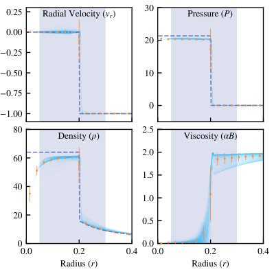
The Noh 1987 problem is known to be extremely challenging, particularly for particle-based codes, and generally requires a high particle number to correctly capture due to an unresolved convergence point. It tests a converging flow that results in a strong radial shock. This is an extreme, idealised, version of an accretion shock commonly present within galaxy formation simulations.
5.4.1 Initial Conditions
There are many ways to generate initial conditions, from very simple schemes to schemes that attempt to highly optimise the particle distribution (Rosswog 2020a, see e.g.). Here, we use a simple initial condition, employing a body-centred cubic lattice distribution of particles in a periodic box. The velocity of the particles is then set such that there is a convergent flow towards the centre of the box,
| (38) |
with , where is the box side-length, the coordinate at the centre of the volume. This gives every particle a speed of unity, meaning those in the centre will have extremely high relative velocities. We cap the minimal value of to be to prevent a singularity at small radii.
The simulation is performed in a dimensionless co-ordinate system, with a box-size of .
5.4.2 Results

The state of the simulation is shown at time in Fig. 9 and visualised in Fig. 10, which shows the radial velocity, which should be zero inside of the shocked region (high density in Fig. 10), and the same as the initial conditions (i.e. -1 everywhere) elsewhere. This behaviour is captured well, with a small amount of scatter, corresponding to the small radial variations in density shown in the image.
The profile of density as a function of radius is however less well captured, with some small waves created by oscillations in the artificial viscosity parameter (see e.g. Rosswog 2020b, for a scheme that corrects for these errors). This can also be seen in the density slice, and is a small effect that also is possibly exacerbated by our non-perfect choice of initial conditions, but is also present in the implementation shown in Rosswog 2020a. The larger, more significant, density error is shown inside the central part of the shocked, high-density, region. This error is ever-present in SPH schemes, and is likely due to both a lack of artificial conduction in this central region (as indicated by Noh 1987, note the excess pressure in the centre caused by ‘wall heating’) and the unresolved point of flow convergence.
The Noh problem converges well using Sphenix, with better than linear convergence for the radial velocity (Fig. 11; recall that for shocks SPH is expected to converge with ).
This problem does not activate the artificial conduction in the Sphenix implementation because of the presence of Equation 34 reducing conductivity in highly viscous flows, as well as our somewhat conservative choice for artificial conduction coefficients (see Appendix E for more details on this topic). However, as these are necessary for the practical functioning of the Sphenix scheme in galaxy formation simulations, and due to this test being highly artificial, this outcome presents little concern.
5.5 Square Test
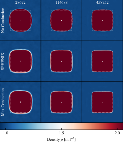
The square test, first presented in Saitoh & Makino 2013, is a particularly challenging test for schemes like Sphenix that do not use a smoothed pressure in their equation of motion, as they typically lead to an artificial surface tension at contact discontinuities (the same ones that lead to the pressure blip in §5.1). This test is a more challenging variant of the ellipsoid test presented in Heß & Springel 2010, as the square includes sharp corners which are more challenging for conduction schemes to capture.
5.5.1 Initial conditions
The initial conditions are generated using equal mass particles. We set up a grid in 2D space with particles, in a box of size . The central square is set to have a density of , and so is replaced with a grid with particles, with the outer region having . The pressures are set to be equal with , with this enforced by setting the internal energies of the particles to their appropriate values. All particles are set to be completely stationary in the initial conditions with . The initial conditions are not allowed to relax in any way.
5.5.2 Results
Fig. 12 shows the square test at for four different resolution levels and three different variations on the Sphenix scheme. By this time the solutions are generally very stable. The top row shows the Sphenix scheme without any artificial conduction enabled (this is achieved by setting to zero) and highlights the typical end state for a Density-Energy SPH scheme on this problem. Artificial surface tension leads to the square deforming and rounding to become more circular.
The bottom row shows the Sphenix scheme with the artificial conduction switch removed; here is set to the same value as . The artificial conduction scheme significantly reduces the rounding of the edges, with a rapid improvement as resolution increases. The rounding present here only occurs in the first few steps as the energy outside the square is transferred to the boundary region to produce a stable linear gradient in internal energy.
Finally, the central row shows the Sphenix scheme, which gives a result indistinguishable from the maximum conduction scenario. This is despite the initial value for the conduction coefficient , meaning it must ramp up rapidly to achieve such a similar result. The Sphenix result here shows that the choices for the conduction coefficients determined from the Sod tube (§5.1) are not only appropriate for that test, but apply more generally to problems that aim to capture contact discontinuities.
5.6 2D Kelvin-Helmholtz Instability

The two dimensional Kelvin-Helmholtz instability is presented below. This test is a notable variant on the usual Kelvin-Helmholtz test as it includes a density jump at constant pressure (i.e. yet another contact discontinuity). This version of the Kelvin-Helmholtz instability is performed in two dimensions. A recent, significantly more detailed, study of Kelvin-Helmholtz instabilities within SPH is available in Tricco 2019. In this section we focus on qualitative comparisons and how the behaviour of the instability changes with resolution within Sphenix.
5.6.1 Initial conditions
The initial conditions presented here are similar to those in Price 2008, where they discuss the impacts more generally of the inclusion of artificial conduction on fluid mixing instabilities. This is set up in a periodic box of length , with the central band between set to and , with the outer region having and to set up a shear flow. The pressure is enforced by setting the internal energies of the equal mass particles. Particles are initially placed on a grid with equal separations. This is the most challenging version of this test for SPH schemes to capture as it includes a perfectly sharp contact discontinuity; see Agertz et al. 2007 for more information.
We then excite a specific mode of the instability, as in typical SPH simulations un-seeded instabilities are dominated by noise and are both unpredictable and unphysical, preventing comparison between schemes.
5.6.2 Results
Fig. 13 shows the simulation after various multiples of the Kelvin-Helmholtz timescale for the excited instability, with given by
| (39) |
where is the density contrast, the shear velocity, and the wavelength of the seed perturbation along the horizontal axis (Hu et al. 2014, e.g). The figure shows three initial resolution levels, increasing from left to right. Despite this being the most challenging version of the Kelvin-Helmholtz test (at this density contrast) for a Density-Energy based SPH scheme, the instability is captured well at all resolutions, with higher resolutions allowing for more rolls of the ‘swirl’ to be captured. In particular, the late-time highly mixed state shows that with the conduction removed after a linear gradient in internal energy has been established, the Sphenix scheme manages to preserve the initial contact discontinuity well. Due to the presence of explicit artificial conduction, Sphenix seems to diffuse more than other schemes on this test (Hu et al. 2014; Wadsley et al. 2017, e.g.), leading to the erausre of some small-scale secondary instabilities.
The non-linear growth rate of the swirls is resolution dependent within this test, with higher-resolution simulations showing faster growth of the largest-scale modes. This is due to better capturing of the energy initially injected to perturb the volume to produce the main instability, with higher resolutions showing lower viscous losses.

Fig. 14 shows a different initial condition where the density contrast , four times higher than the one initially presented. Because SPH is fundamentally a finite mass method, and we use equal-mass particles throughout, this is a particularly challenging test as the low-density region is resolved by so few particles. Here we also excite an instability with a wavelength , four times smaller than the one used for the test. This value is chosen for two reasons; it is customary to lower the wavelength of the seeded instability as the density contrast is increased when grid codes perform this test as it allows each instability to be captured with the same number of cells at a given resolution level; and also to ensure that this test is as challenging as is practical for the scheme.
Sphenix struggles to capture the instability at very low resolutions primarily due to the lack of particles in the low-density flow (Price 2008, an issue also encountered by). In the boundary region the artificial conduction erases the small-scale instabilities on a timescale shorter than their formation timescale (as the boundary region is so large) and as such they cannot grow efficiently. As the resolution increases, however, Sphenix is able to better capture the linear evolution of the instability, even capturing turn-overs and the beginning of nonlinear evolution for the highest resolution.
5.7 Blob Test

The Blob test is a challenging test for SPH schemes (Klein et al. 1994; Springel 2005, see ) and aims to replicate a scenario where a cold blob of gas falls through the hot IGM/CGM surrounding a galaxy. In this test, a dense sphere of cold gas is placed in a hot, low density, and supersonic wind. Ideally, the blob should break up and dissolve into the wind, but Agertz et al. 2007 showed that the inability of traditional SPH schemes to exchange entropy between particles prevents this from occurring. The correct, specific, rate at which the blob should mix with its surroundings, as well as the structure of the blob whilst it is breaking up, are unknown.
5.7.1 Initial Conditions
There are many methods to set up the initial conditions for the Blob test, including some that excite an instability to ensure that the blob breaks up reliably (Hu et al. 2014, such as those used in). Here we excite no such instabilities and simply allow the simulation to proceed from a very basic particle set-up with a perfectly sharp contact discontinuity. The initial conditions are dimensionless in nature, as the problem is only specified in terms of the Mach number of the background medium and the blob density contrast.
To set up the initial particle distribution, we use two body centred cubic lattices, one packed at a high-density (for the blob, ) and one at low density (for the background medium, ). The low-density lattice is tiled four times in the direction to make a box of size , and at a sphere of radius is removed and filled in with particles from the high-density lattice. The particles in the background region are given a velocity of (with the blob being stationary), and the internal energy of the gas everywhere is scaled such that the background medium has a mach number of and the system is in pressure equilibrium everywhere.
5.7.2 Results
The blob is shown at a number of resolution levels at various times in Fig. 15. At all resolution levels the blob mixes well with the background medium after a few Kelvin-Helmholtz timescales (see Eqn. 39 for how this is calculated; here we assume that the wavelength of the perturbation is the radius of the blob)66 6 Note that here the Kelvin-Helmholtz timescale is 1.1 times the cloud crushing timescale (Agertz et al. 2007). . The rate of mixing is consistent amongst all resolution levels, implying that the artificial conduction scheme is accurately capturing unresolved mixing at lower resolutions.
The rate of mixing of the blob is broadly consistent with that of modern SPH schemes and grid codes, however our set of initial conditions appear to mix slightly slower (taking around to fully mix) than those used by other contemporary works (Agertz et al. 2007; Read & Hayfield 2012; Hu et al. 2014), possibly due to the lack of perturbation seeding (see Read et al. 2010, Appendix B for more details). When testing these initial conditions with a scheme that involves a Riemann solver or a Pressure-based scheme (see Appendix F) the rate of mixing is qualitatively similar to the one presented here. Sphenix is unable to fully capture the crushing of the blob from the centre outwards seen in grid codes and other SPH formulations using different force expressions (Wadsley et al. 2017), rather preferring to retain a ‘plate’ of dense gas at the initial point of the blob that takes longer to break up. A potential explanation for this difference is some residual surface tension in Sphenix. In these highly dynamic situations, it may not be possible for the artificial conduction to establish a smooth internal energy profile rapidly enough for small-scale instabilities on the surface to assist in the breakup of the blob.
At low resolutions it is extremely challenging for the method to capture the break-up of the blob as there are very few particles in the background medium to interact with the blob due to the factor of 10 density contrast.

5.8 Evrard Collapse
The Evrard collapse (Evrard 1988) test takes a large sphere of self-gravitating gas, at low energy and density, that collapses in on itself, causing an outward moving accretion shock. This test is of particular interest for cosmological and astrophysical applications as it allows for the inspection of the coupling between the gravity and hydrodynamics solver.
5.8.1 Initial Conditions
Gas particles are set up in a sphere with an adiabatic index of , sphere mass , sphere radius , initial density profile , and in a very cold state with , with the gravitational constant . These initial conditions are created in a box of size 100, ensuring that effects from the periodic boundary are negligible. Unfortunately, due to the non-uniform density profile, it is considerably more challenging to provide relaxed initial conditions (or use a glass file). Here, positions are simply drawn randomly to produce the required density profile.
The Evrard collapse was performed at four resolution levels, with total particle numbers in the sphere being , , , and . The gravitational softening was fixed at for the resolution level, and this was scaled with with the particle mass for the other resolution levels. The simulations were performed once with artificial conduction enabled (the full Sphenix scheme), and once with it disabled.
5.8.2 Results
The highest resolution result ( particles) with the full Sphenix scheme is shown in Fig. 16. This is compared against a high resolution grid code77 7 HydroCode1D, see https://github.com/bwvdnbro/HydroCode1D and the Swift repository for more details. simulation performed in 1D, and here Sphenix shows an excellent match to the reference solution. The shock at around is sharply resolved in all variables, and the density and velocity profiles show excellent agreement. In the centre of the sphere, there is a slight deviation from the reference solution for the internal energy and density (balanced to accurately capture the pressure in this region) that remains even in the simulation performed without artificial conduction (omitted for brevity, as the simulation without conduction shows similar results to the simulation with conduction, with the exception of the conduction reducing scatter in the internal energy profile). This is believed to be an artefact of the initial conditions, however it was not remedied by performing simulations at higher resolutions.
The convergence properties of the Evrard sphere are shown in Fig. 17. The velocity profile shows a particularly excellent result, with greater than linear convergence demonstrated. The thermodynamic properties show roughly linear convergence. Of particular note is the difference between the convergence properties of the simulations with and without artificial conduction; those with this feature of Sphenix enabled converge at a more rapid rate. This is primarily due to the stabilising effect of the conduction on the internal energy profile. As the particles are initially placed randomly, there is some scatter in the local density field at all radii. This is quickly removed by adiabatic expansion in favour of scatter in the internal energy profile, which can be stabilised by the artificial conduction.
5.9 nIFTy Cluster

The nIFTy cluster comparison project, Sembolini et al. 2016, uses a (non-radiative, cosmological) cluster-zoom simulation to evaluate the efficacy of various hydrodynamics and gravity solvers. The original paper compared various types of schemes, from traditional SPH (Springel 2005, Gadget,) to a finite volume adaptive mesh refinement scheme (Teyssier 2002, RAMSES,). The true answer for this simulation is unknown, but it is a useful case to study the different characteristics of various hydrodynamics solvers.
In Fig. 18 the Sphenix scheme is shown with and without artificial conduction against three reference schemes from Sembolini et al. 2016. Here, the centre the cluster was found using the VELOCIraptor (Elahi et al. 2019) friends-of-friends halo finder, and the particle with the minimum gravitational potential was used as the reference point.
The gas density profile was created using 25 equally log-spaced radial bins, with the density calculated as the sum of the mass within a shell divided by the shell volume. Sphenix scheme shows a similar low-density core as AREPO, with the no conduction scheme resulting in a cored density profile similar to the traditional SPH scheme from Sembolini et al. 2016.
The central panel of Fig. 18 shows the ‘entropy’ profile of the cluster; this is calculated as with the electron density (assuming primordial gas, this is with the mass of a hydrogen atom) and the gas temperature. Each was calculated individually in the same equally log-spaced bins as the density profile, with the temperature calculated as the mass-weighted temperature within that shell. The rightmost panel shows this mass-weighted temperature profile, with Sphenix showing slightly higher temperatures in the central region than AREPO, matching G2-anarchy instead. This high-temperature central region, along with a low-density centre, lead to the ‘cored’ (i.e. flat, with high values of entropy, at small radii) entropy profile for Sphenix.
The cored central entropy profile with Sphenix is attained primarily due to the artificial conduction scheme and is not due to the other improvements over the traditional SPH base scheme (including for example the artificial viscosity implementation). We note again that there was no attempt to calibrate the artificial conduction scheme to attain this result on the nIFTy cluster, and any and all parameter choices were made solely based on the Sod shock tube in §5.1.
In Fig. 19, a projected mass-weighted temperature image of the cluster is shown. The image demonstrates how the artificial conduction present in the Sphenix scheme promotes phase mixing, resulting in the cored entropy profile demonstrated in Fig. 18.
The temperature distribution in the SPH simulation without conduction appears noisier, due to particles with drastically different phases being present within the same kernel. This shows how artificial conduction can lead to sharper shock capture as the particle distribution is less susceptible to this noise, enabling a cleaner energy transition between the pre- and post-shock region.
6 Conclusions
We have presented the Sphenix SPH scheme and its performance on seven hydrodynamics tests. The scheme has been demonstrated to show convergent (with resolution) behaviour on all these tests. In summary:
- •
Sphenix is an SPH scheme that uses Density-Energy SPH as a base, with added artificial viscosity for shock capturing and artificial conduction to reduce errors at contact discontinuities and to promote phase mixing.
- •
A novel artificial conduction limiter allows Sphenix to be used with energy injection feedback schemes (such as those used in EAGLE) by reducing conduction across shocks and other regions where the artificial viscosity is activated.
- •
The artificial viscosity and conduction scheme coefficients were determined by ensuring good performance on the Sod Shock tube test, and remain fixed for all other tests.
- •
The modified Inviscid SPH (Cullen & Dehnen 2010) scheme captures strong shocks well, ensuring energy conservation, as shown by the Sedov-Taylor blastwave test, but the smooth nature of SPH prevents rapid convergence with resolution.
- •
The use of the Balsara 1989 switch in Sphenix was shown to be adequate to ensure that the Gresho-Chan vortex is stable. Convergence on this test was shown to be faster than in Cullen & Dehnen 2010.
- •
The artificial conduction scheme was shown to work adequately to capture thermal instabilities in both the Kelvin-Helmholtz and Blob tests, with contact discontinuities well preserved when required.
- •
Sphenix performed well on both the Evrard collapse and nIFTY cluster problems, showing that it can couple to the FMM gravity solver in Swift and that the artificial conduction scheme can allow for entropy cores in clusters.
- •
Sphenix is implemented in the Swift code and is available fully open source to the community.
Sphenix hence achieves its design goals; the Lagrangian nature of the scheme allows for excellent coupling with gravity; the artificial conduction limiter allows the injection of energy as in the EAGLE sub-grid physics model; and the low cost-per-particle and lack of matrices carried on a particle-by-particle basis provide for a very limited computational cost (see Borrow et al. 2019, for a comparison of computational costs between a scheme like Sphenix and the GIZMO-like schemes also present in Swift).
7 Acknowledgements
The authors thank Folkert Nobels for providing initial conditions for Appendix C, and the anonymous referee for their comments that improved the paper. JB is supported by STFC studentship ST/R504725/1. MS is supported by the Netherlands Organisation for Scientific Research (NWO) through VENI grant 639.041.749. RGB is supported by the Science and Technology Facilities Council ST/P000541/1. This work used the DiRAC@Durham facility managed by the Institute for Computational Cosmology on behalf of the STFC DiRAC HPC Facility (www.dirac.ac.uk). The equipment was funded by BEIS capital funding via STFC capital grants ST/K00042X/1, ST/P002293/1, ST/R002371/1 and ST/S002502/1, Durham University and STFC operations grant ST/R000832/1. DiRAC is part of the National e-Infrastructure.
7.1 Software Citations
This paper made use of the following software packages:
- •
Swift (Schaller et al. 2018)
- •
python (van Rossum & Drake Jr 1995), with the following libraries
- –
numpy (Harris et al. 2020)
- –
- –
numba (Lam et al. 2015)
- –
matplotlib (Hunter 2007)
- –
swiftsimio (Borrow & Borrisov 2020)
- –
8 Data Availability
All code and initial conditions used to generate the simulations is open source as part of Swift version 0.9.0 (Schaller et al. 2018)88 8 Available from http://swift.dur.ac.uk, https://gitlab.cosma.dur.ac.uk/swift/swiftsim, and https://github.com/swiftsim/swiftsim. . As the simulations presented in this paper are small, test, simulations that can easily be repeated, the data is not made immediately available.
References
- Agertz et al. (2007) Agertz O., et al., 2007, Monthly Notices of the Royal Astronomical Society, 380, 963
- Balsara (1989) Balsara D. S., 1989, PhD thesis
- Bauer & Springel (2012) Bauer A., Springel V., 2012, Monthly Notices of the Royal Astronomical Society, 423, 2558
- Benz (1988) Benz W., 1988, Computer Physics Communications, 48, 97
- Borrow & Borrisov (2020) Borrow J., Borrisov A., 2020, Journal of Open Source Software, 5, 2430
- Borrow et al. (2018) Borrow J., Bower R. G., Draper P. W., Gonnet P., Schaller M., 2018, Proceedings of the 13th SPHERIC International Workshop, Galway, Ireland, June 26-28 2018, pp 44–51
- Borrow et al. (2019) Borrow J., Vandenbroucke B., Schaller M., 2019, in Proceedings of the 14th SPHERIC International Workshop, Exeter, United Kingdom, June 25-27 2019. Exeter, United Kingdom
- Borrow et al. (2020) Borrow J., Schaller M., Bower R. G., 2020, arXiv e-prints, p. arXiv:2011.11641
- Cen (1992) Cen R., 1992, The Astrophysical Journal Supplement Series, 78, 341
- Cen & Ostriker (1992) Cen R., Ostriker J. P., 1992, \apjl, 399, L113
- Courant et al. (1928) Courant R., Friedrichs K., Lewy H., 1928, Mathematische Annalen, 100, 32
- Crain et al. (2007) Crain R. A., Eke V. R., Frenk C. S., Jenkins A., McCarthy I. G., Navarro J. F., Pearce F. R., 2007, Monthly Notices of the Royal Astronomical Society, 377, 41
- Cullen & Dehnen (2010) Cullen L., Dehnen W., 2010, Monthly Notices of the Royal Astronomical Society, 408, 669
- Dalla Vecchia & Schaye (2008) Dalla Vecchia C., Schaye J., 2008, Monthly Notices of the Royal Astronomical Society, 387, 1431
- Dalla Vecchia & Schaye (2012) Dalla Vecchia C., Schaye J., 2012, Monthly Notices of the Royal Astronomical Society, 426, 140
- Debackere et al. (2020) Debackere S. N. B., Schaye J., Hoekstra H., 2020, Monthly Notices of the Royal Astronomical Society, 492, 2285
- Dehnen (2014) Dehnen W., 2014, Computational Astrophysics and Cosmology, 1, 1
- Dehnen & Aly (2012) Dehnen W., Aly H., 2012, Monthly Notices of the Royal Astronomical Society, 425, 1068
- Dolag et al. (2004) Dolag K., Jubelgas M., Springel V., Borgani S., Rasia E., 2004, The Astrophysical Journal, 606, L97
- Durier & Dalla Vecchia (2012) Durier F., Dalla Vecchia C., 2012, Monthly Notices of the Royal Astronomical Society, 419, 465
- Elahi et al. (2019) Elahi P. J., Cañas R., Poulton R. J. J., Tobar R. J., Willis J. S., Lagos C. d. P., Power C., Robotham A. S. G., 2019, Publications of the Astronomical Society of Australia, 36, e021
- Ettori et al. (2006) Ettori S., Dolag K., Borgani S., Murante G., 2006, Monthly Notices of the Royal Astronomical Society, 365, 1021
- Evrard (1988) Evrard A. E., 1988, Monthly Notices of the Royal Astronomical Society, 235, 911
- Gingold & Monaghan (1977) Gingold R. A., Monaghan J. J., 1977, Monthly Notices of the Royal Astronomical Society, 181, 375
- Greengard & Rokhlin (1987) Greengard L., Rokhlin V., 1987, Journal of Computational Physics, 73, 325
- Gresho & Chan (1990) Gresho P. M., Chan S. T., 1990, International Journal for Numerical Methods in Fluids, 11, 621
- Gresho & Sani (1990) Gresho P. M., Sani R. L., 1990, International Journal for Numerical Methods in Fluids, 11, 951
- Guillet et al. (2019) Guillet T., Pakmor R., Springel V., Chandrashekar P., Klingenberg C., 2019, Monthly Notices of the Royal Astronomical Society, 485, 4209
- Harris et al. (2020) Harris C. R., et al., 2020, arXiv e-prints, p. arXiv:2006.10256
- Hernquist & Katz (1989) Hernquist L., Katz N., 1989, The Astrophysical Journal Supplement Series, 70, 419
- Heß & Springel (2010) Heß S., Springel V., 2010, Monthly Notices of the Royal Astronomical Society, 406, 2289
- Hopkins (2013) Hopkins P. F., 2013, Monthly Notices of the Royal Astronomical Society, 428, 2840
- Hopkins (2015) Hopkins P. F., 2015, Monthly Notices of the Royal Astronomical Society, 450, 53
- Hu et al. (2014) Hu C.-Y., Naab T., Walch S., Moster B. P., Oser L., 2014, Monthly Notices of the Royal Astronomical Society, 443, 1173
- Hunter (2007) Hunter J. D., 2007, Computing in Science & Engineering, 9, 90
- Klein et al. (1994) Klein R. I., McKee C. F., Colella P., 1994, The Astrophysical Journal, 420, 213
- Lam et al. (2015) Lam S. K., Pitrou A., Seibert S., 2015, in Proceedings of the Second Workshop on the LLVM Compiler Infrastructure in HPC. LLVM ’15. Association for Computing Machinery, New York, NY, USA, doi:10.1145/2833157.2833162
- Lattanzio et al. (1986) Lattanzio J. C., Monaghan J. J., Pongracic H., Schwarz M. P., 1986, SIAM Journal on Scientific and Statistical Computing, 7, 591
- Lucy (1977) Lucy L. B., 1977, The Astronomical Journal, 82, 1013
- Monaghan (1992) Monaghan J. J., 1992, Annual Review of Astronomy and Astrophysics, 30, 543
- Monaghan (1997) Monaghan J., 1997, Journal of Computational Physics, 136, 298
- Monaghan (2002) Monaghan J. J., 2002, Monthly Notices of the Royal Astronomical Society, 335, 843
- Monaghan & Gingold (1983) Monaghan J., Gingold R., 1983, Journal of Computational Physics, 52, 374
- Morris & Monaghan (1997) Morris J., Monaghan J., 1997, Journal of Computational Physics, 136, 41
- Navarro & White (1993) Navarro J. F., White S. D. M., 1993, \mnras, 265, 271
- Navarro et al. (1996) Navarro J. F., Frenk C. S., White S. D. M., 1996, The Astrophysical Journal, 462, 563
- Noh (1987) Noh W. F., 1987, Journal of Computational Physics, 72, 78
- Oppenheimer et al. (2018) Oppenheimer B. D., Schaye J., Crain R. A., Werk J. K., Richings A. J., 2018, Monthly Notices of the Royal Astronomical Society, 481, 835
- Ploeckinger & Schaye (2020) Ploeckinger S., Schaye J., 2020, Monthly Notices of the Royal Astronomical Society, 497, 4857
- Price (2007) Price D. J., 2007, Publications of the Astronomical Society of Australia, 24, 159
- Price (2008) Price D. J., 2008, Journal of Computational Physics, 227, 10040
- Price (2012) Price D. J., 2012, Journal of Computational Physics, 231, 759
- Price et al. (2018) Price D. J., et al., 2018, Publications of the Astronomical Society of Australia, 35, e031
- Read & Hayfield (2012) Read J. I., Hayfield T., 2012, Monthly Notices of the Royal Astronomical Society, 422, 3037
- Read et al. (2010) Read J. I., Hayfield T., Agertz O., 2010, Monthly Notices of the Royal Astronomical Society, pp no–no
- Revaz & Jablonka (2012) Revaz Y., Jablonka P., 2012, Astronomy & Astrophysics, 538, A82
- Rosswog (2020a) Rosswog S., 2020a, Monthly Notices of the Royal Astronomical Society, 498, 4230
- Rosswog (2020b) Rosswog S., 2020b, The Astrophysical Journal, 898, 60
- Saitoh & Makino (2009) Saitoh T. R., Makino J., 2009, ApJ, 697, L99
- Saitoh & Makino (2013) Saitoh T. R., Makino J., 2013, The Astrophysical Journal, 768, 44
- Schaller et al. (2015) Schaller M., Dalla Vecchia C., Schaye J., Bower R. G., Theuns T., Crain R. A., Furlong M., McCarthy I. G., 2015, Monthly Notices of the Royal Astronomical Society, 454, 2277
- Schaller et al. (2016) Schaller M., Gonnet P., Chalk A. B. G., Draper P. W., 2016, Proceedings of the Platform for Advanced Scientific Computing Conference on - PASC ’16, pp 1–10
- Schaller et al. (2018) Schaller M., Gonnet P., Draper P. W., Chalk A. B. G., Bower R. G., Willis J., Hausammann L., 2018, Astrophysics Source Code Library, p. ascl:1805.020
- Schaye & Dalla Vecchia (2008) Schaye J., Dalla Vecchia C., 2008, \mnras, 383, 1210
- Schaye et al. (2015) Schaye J., et al., 2015, Monthly Notices of the Royal Astronomical Society, 446, 521
- SciPy 1.0 Contributors et al. (2020) SciPy 1.0 Contributors et al., 2020, Nature Methods, 17, 261
- Sedov (1959) Sedov 1959, Similarity and Dimensional Methods in Mechanics - NASA/ADS
- Sembolini et al. (2016) Sembolini F., et al., 2016, Monthly Notices of the Royal Astronomical Society, 457, 4063
- Sod (1978) Sod G. A., 1978, Journal of Computational Physics, 27, 1
- Springel (2005) Springel V., 2005, Monthly Notices of the Royal Astronomical Society, 364, 1105
- Springel (2010) Springel V., 2010, Monthly Notices of the Royal Astronomical Society, 401, 791
- Springel & Hernquist (2002) Springel V., Hernquist L., 2002, Monthly Notices of the Royal Astronomical Society, 333, 649
- Springel & Hernquist (2003) Springel V., Hernquist L., 2003, Monthly Notices of the Royal Astronomical Society, 339, 289
- Stern et al. (2019) Stern J., Fielding D., Faucher-Giguère C.-A., Quataert E., 2019, arXiv:1906.07737 [astro-ph]
- Taylor (1950) Taylor G., 1950, Proceedings of the Royal Society of London Series A, 201, 159
- Teyssier (2002) Teyssier R., 2002, Astronomy & Astrophysics, 385, 337
- Tricco (2019) Tricco T. S., 2019, \mnras, 488, 5210
- Vila (1999) Vila J. P., 1999, Mathematical models and methods in applied sciences, 9, 161
- Wadsley et al. (2004) Wadsley J., Stadel J., Quinn T., 2004, New Astronomy, 9, 137
- Wadsley et al. (2008) Wadsley J. W., Veeravalli G., Couchman H. M. P., 2008, Monthly Notices of the Royal Astronomical Society, 387, 427
- Wadsley et al. (2017) Wadsley J. W., Keller B. W., Quinn T. R., 2017, Monthly Notices of the Royal Astronomical Society, 471, 2357
- Weinberger et al. (2020) Weinberger R., Springel V., Pakmor R., 2020, The Astrophysical Journal Supplement Series, 248, 32
- Wendland (1995) Wendland H., 1995, Advances in Computational Mathematics, 4, 389
- Wiersma et al. (2009) Wiersma R. P. C., Schaye J., Theuns T., Dalla Vecchia C., Tornatore L., 2009, Monthly Notices of the Royal Astronomical Society, 399, 574
- Wood (1981) Wood D., 1981, Monthly Notices of the Royal Astronomical Society, 194, 201
- van Rossum & Drake Jr (1995) van Rossum G., Drake Jr F. L., 1995, in , Vol. 620, Python Tutorial. Centrum voor Wiskunde en Informatica, Amsterdam
Appendix A Particle Costs
Different SPH models require different information stored per particle. Compared to a basic, ‘Traditional’ SPH model, Sphenix requires a small amount of extra data to store things like the particle-carried artificial conduction and viscosity coefficients. The amount of data required increases for more complex models, such as those making use of the full shear tensor, like Wadsley et al. 2017, or additional corrections, like Rosswog 2020b. SPH models using an ALE (Arbitrary Lagrangian-Eulerian) framework (Vila 1999, see) require even more information as the particles carry flux information for use in the Riemann solver.
The amount of data required to store a single element in memory is of upmost importance when considering the speed at which a simulation will run. SPH codes, and Swift in particular, are bound by the memory bandwidth available, rather than the costs associated with direct computation. This means any increase in particle cost corresponds to a linear increase in the required computing time for simulation; this is why keeping the particles lean is a key requirement of the Sphenix model. Additionally, in large simulations performed over many nodes, the bandwidth of the interconnect can further become a limitation and hence keeping the memory cost of particles low is again beneficial.
In Fig. 20 we show the memory cost of four models: Traditional SPH (Springel 2005, similar to to the one implemented in Gadget-2;), Sphenix, a model with the full shear matrix, and a SPH-ALE model similar to GIZMO-MFM (Hopkins 2015), all implemented in the Swift framework. We see that Sphenix only represents a 25% increase in memory cost per particle for significant improvement over the traditional model.
Appendix B Conduction Speed

The conduction speed (Eqn. 26) in Sphenix was primarily selected for numerical reasons. In a density based scheme, it is common to see significant errors around contact discontinuities where there are large changes in density and internal energy simultaneously to produce a uniform pressure field. In Fig. 3 we demonstrated the performance of the Sphenix scheme on one of these discontinuities, present in the Sod Shock.
In Fig. 21 we zoom in on the contact discontinuity, this time using glass files for the base initial conditions (of resolution and ), allowing for a more even distribution of particles along the horizontal axis. We use five different models,
- •
Sphenix, the full Sphenix model using the conduction speed from Eqn. 26.
- •
Pressure Term, which uses only the pressure-based term from Eqn. 26.
- •
Velocity Term, which only uses the velocity-based term from Eqn. 26.
- •
No Conduction, which sets the conduction speed to zero.
- •
Max Conduction, which sets to unity everywhere, and uses the conduction speed from Eqn. 26.
The first thing to note here is that the pressure term provides the vast majority of the conduction speed, highlighting the importance of this form of bulk conduction in Sphenix and other models employing a density based equation of motion. Importantly, the conduction allows for the ‘pressure blip’ to be reduced to a level where there is no longer a discontinuity in pressure (i.e. there is a smooth gradient with ). Although the velocity term is able to marginally reduce the size of the blip relative to the case without conduction, it is unable to fully stabilise the solution alone. Pressure blips can lead to large pressure differences between individual particles, then leading to the generation of a divergent flow around the point where the contact discontinuity resides. This is the primary motivation for the inclusion of the velocity divergence-based term in the conduction speed. Along with the conduction limiter (see Eqn. 28 for the source term), if there is a large discontinuity in internal energy that is generating a divergent flow (and not one that is expected to do so, such as a shock), the velocity-dependent term can correct for this and smooth out the internal energy until the source of divergence disappears.
B.1 Alternative Conduction Speeds
The Sphenix conduction speed (Eqn. 26) contains two components: one based on pressure differences and one based on a velocity component. In Sphenix, as in a number of other models, this velocity component really encodes compression or expansion along the axis between particles.
The motivation for some alternative schemes (Wadsley et al. 2008; Wadsley et al. 2017, e.g. those presented in) is shear between particles. To test if we see significant differences in our tests, we formulate a new conduction speed,
| (40) |
that focuses on capturing the shear component of the velocity between two particles.

We again test this new formulation on some of our example problems. First, the nIFTy cluster, presented in Fig. 22, shows little difference between the two formulations, with both providing a solution similar to other modern SPH schemes and grid codes.
The Kelvin-Helmholtz test again shows little difference (Fig. 23), although there is a slightly increased growth rate of the perturbation at late times for the shear formulation.
We find no discernible difference between the two formulations on the blob test, as this is mainly limited by the choice of Density-SPH as the base equation of motion to correctly capture the initial break up of the blob from the centre outwards.
Appendix C Maintenance of Hydrostatic Balance

The form of the conduction speed used in Sphenix based on pressure differences (Eqn. 26) has been conjectured to not allow for the maintenance of a pressure gradient against some external body force (Sembolini et al. 2016, for example a halo in hydrostatic equilibrium;). The main concern here is that the pressure difference form of the conduction speed may allow thermal energy to travel down into the gravitational potential, heating the central regions of the halo. As Sphenix uses an additional limiter (Eqn. 28 for the source term) that only activates conduction in regions where the internal energy gradient cannot be represented by SPH anyway, this may be less of a concern. Additionally, there will be no conduction across accretion shocks due to the limiter in Eqn. 33.
In Fig. 24 we show an idealised simulation of an adiabatic halo with an NFW (Navarro et al. 1996) dark matter density profile, and gas in hydrostatic equilibrium. The halo uses a fixed NFW potential in the background, with a mass of M⊙, concentration , and a stellar bulge fraction of 1%. The halo has a gas mass of M⊙, resolved by 1067689 particles with varying mass from to M⊙ with the highest resolution in the centre.
The gas in the halo is set up to be isothermal, following (Stern et al. 2019),
| (41) |
where is the circular velocity of the halo. The condition used to set the initial temperatures is , and to get the correct normalisation for pressure and density the gas fraction at is used following Debackere et al. 2020.
Fig. 24 shows that there is little difference between the result with conduction, and without. There is a small offset in the centre where the simulation with conduction has a slightly higher energy and slightly lower density, giving a very small overall offset in pressure. This figure is shown at Gyr, much longer than any realistic cluster of a similar mass would go without accretion or some other external force perturbing the pressure profile anyway. Finally, the conduction allows the noisy internal energy distribution (and additionally density distribution) to be normalised over time thanks to the inclusion of the pressure differencing term.
Appendix D Sedov Blast

In Fig. 6 we presented the convergence properties of the Sedov blast with the Sphenix scheme. The scheme only demonstrated convergence as , which is much slower than the expected convergence rate of for shock fronts in SPH (that is demonstrated and exceeded in the Noh problem in Fig. 11). This is, however, simply an artefact of the way that the convergence is measured.
In Fig. 25 we show the actual density profiles of the shock front, by resolution (increasing as the subfigures go to the right). Note here that the width of the shock front (from the particle distribution to the right of the vertical line to the vertical line in the analytical solution) does converge at the expected rate of with the number of particles in the volume (in 3D).
The Sedov blast, unlike the Noh problem and Sod tubes, does not aim to reproduce a simple step function in density and velocity, but also a complex, expanding, post-shock region. The convergence is measured ‘vertically’ in this figure, but it is clear here that the vertical deviation from the analytical solution is not representative of the ‘error’ in the properties of a given particle, or in the width of the shock front. Small deviations in the position of the given particle could result in changes of orders of magnitude in the value of the norm measured for it.
Because of this, and because we have demonstrated in other sections that Sphenix is able to converge on shock problems at faster than first order, we believe the slow convergence on the Sedov problem to be of little importance in practical applications of the scheme.
Appendix E Conduction in the Noh Problem

In §5.4 we presented the Noh problem, and showed that the Sphenix scheme (like other SPH schemes in general) struggles to capture the high density in the central region due to so-called ‘wall heating’.
The Sphenix scheme includes a switch to reduce artificial conduction in viscous flows. This is, as presented in §4, to allow for the capturing of energetic feedback events. It does, however, lead to a minor downside; the stabilising effect of the conduction in these shocks is almost completely removed. Usually, the artificial conduction lowers the dispersion in local internal energy values, and hence pressures, allowing for a more regular particle distribution.
In Fig. 26 we show three re-simulations of the Noh problem (at resolution) with three separate schemes. The first, the full Sphenix scheme, is simply a lower resolution version of Fig. 10. The second, ‘No Conduction Limiter’, is the Sphenix scheme, but with Equation 34 removed; i.e. the particle-carried artificial conduction coefficient depends solely on the local internal energy field (through and Eqn. 28), instead of also being mediated by the velocity divergence field. The final case, ‘Fixed ’, shows the case where we remove all conduction switches and use a fixed value for the conduction of . The former two look broadly similar, suggesting that the post-shock region is not significantly affected by the additional Sphenix conduction limiter.
The final panel, however, shows the benefits available to a hypothetical scheme that can remove the artificial conduction switch; the central region is able to hold a significantly higher density thanks to energy being conducted out of this region, allowing the pressure to regularise. In addition to the above, this case shows significantly weaker spurious density features (recall that the post-shock, high-density, region should have a uniform density) because these have been regularised by the conduction scheme.
We present this both to show the drawbacks of the Sphenix artificial conduction scheme, and to show the importance of demonstrating test problems with the same switches that would be used in a production simulation.
Appendix F Blob Test


In Fig. 15 we demonstrated the performance of the Sphenix scheme on an example ‘blob’ test. Here, we show how the same initial conditions are evolved using two schemes: a ‘traditional SPH’ scheme with fixed artificial viscosity () and no artificial conduction (Monaghan 1992, e.g.)99 9 The minimal scheme in Swift., and a SPH-ALE (Vila 1999) scheme similar to GIZMO-MFM1010 10 The gizmo-mfm scheme in Swift with a HLLC Riemann solver. (Hopkins 2015) with a diffusive slope limiter. This is in an effort to demonstrate how the initial conditions are evolved with a minimally viable non-diffusive scheme, through to what could be considered the most diffusive viable scheme.
Fig. 27 shows the result of the blob test with the traditional SPH scheme. Here, as expected, there is a severe lack of mixing, with the artificial surface tension holding the blob together even at the highest resolutions. The lack of phase mixing also contributes to a lack of overall mixing, with the stripped trails (shown most clearly at ) adiabatically expanding but crucially remaining distinct from the hot background medium.
Fig. 28 shows the result of the blob test with the SPH-ALE (GIZMO-MFM) scheme. This scheme is known to be highly diffusive (due to the less conservative slope limiter employed in the Swift implementation). This follows closely the results seen in e.g. Agertz et al. 2007 for diffusive grid-based codes. Here, the blob is rapidly shattered, and then dissolves quickly into the surrounding media, especially at the lowest resolutions.
The Sphenix results in Fig. 15 showed that the blob mixed with the surrounding media, but at a less rapid rate than in the SPH-ALE case. This is somewhat expected, given the trade-off required in the artificial conduction switches (Eqn. 34). We do note, however, that no analytical solution exists for the blob test, and as such all of these comparisons may only be made qualitatively.
In Fig. 29 we examine the effect of removing the conduction limiter from the Sphenix implementation (i.e. Eqn. 34 is removed, allowing to vary irrespective of the values of ). We see that the inclusion of the limiter does slightly reduce the rate of initial mixing within the blob, but that the effect of the limiter is not particularly strong within this case.