Abstract

1. item 11

   Introduction

   Let $d\geq 2$ and $k\geq 1$ be fixed integers. A simple graph $G$ is a finite, unweighted, undirected graph containing no loops or multiple edges. We write $G=(V,E)$, where $V=V(G)$ is a finite set of vertices, and $E=E(G)$ is the set of edges. Throughout the thesis, we will assume $G$ to be a $d$-bounded degree graph, that is, the maximum degree of a vertex in $G$ is upper bounded by $d$. Given two different vertices $u,v\in V$ let $\text{dist}_{G}(u,v)$ be the length of the shortest path between $u$ and $v$.

   For any $v\in V$, the $k$-disc of $v$, denoted by $\text{disc}_{k}(v)$ or $\text{disc}_{k}(G,v)$ is defined as the rooted subgraph in $G$ that is induced by the vertices that are at distance at most $k$ to $v$ in $G$. Two $k$-discs are isomorphic if and only if there exists a root-preserving graph isomorphism between them (a graph isomorphism that identifies the roots). We denote the set of all non-isomorphic $d$-bounded degree rooted graphs with radius at most $k$ by $\mathcal{L}(d,k)$.

   Fact 1.0.1.

   Let $v\in V$ be a vertex, then $|\text{disc}_{k}(v)|\leq 2d^{k}$. In particular $\mathcal{L}(d,k)$ is finite.

   Proof Since $d$ is finite, the amount of vertices in $\text{disc}_{k}(v)$ is at most $1+d+...+d^{k}\leq 2d^{k}$. There is only a finite amount of simple $d$-bounded degree graphs on $2d^{k}$ vertices, and so $\mathcal{L}(d,k)$ is finite.
   
   We denote the size of $\mathcal{L}(d,k)$ by $L\coloneqq L(d,k)$ and write $\mathcal{L}(d,k)=\{\Gamma_{1},...,\Gamma_{L}\}$.

   The $k$-disc count vector $\text{cnt}_{k}(G)$ of a graph $G$ is an $L$-dimensional vector where the $i$-th entry counts the number of $k$-discs in $G$ that are isomorphic to $\Gamma_{i}\in\mathcal{L}(d,k)$. Given a $k$-disc isomorphism type $\Gamma$, $\text{cnt}_{k}(G,\Gamma)$ is defined as the entry in $\text{cnt}_{k}(G)$ that corresponds to $\Gamma$.

   The $k$-disc frequency distribution vector (FDV) of $G$, denoted by $\text{freq}_{k}(G)$, is the vector where the $i$-th entry counts the fraction of $k$-discs in $G$ that are isomorphic to $\Gamma_{i}\in\mathcal{L}(d,k)$, or equivalently $\text{freq}_{k}(G)\coloneqq\text{cnt}_{k}(G)/|V(G)|$.

   Given a $k$-disc isomorphism type $\Gamma$, $\text{freq}_{k}(G,\Gamma)$ is defined as the entry in $\text{freq}_{k}(G)$ that corresponds to $\Gamma$.
   

   The main question, as given by N. Alon in [BER], is whether it is possible to construct a small graph $H$ that has approximately the same local structure as an arbitrarily large simple graph $G$ whose degree is bounded by $d$.

   Question 1.0.2.

   (N. Alon)

   Let $d\geq 2,k\geq 1,\epsilon\in(0,1)$. Is there a computable function $f\coloneqq f(d,k,\epsilon)$ such that for any simple $d$-bounded graph $G$ there is a simple graph $H$ such that

   $$||\text{freq}_{k}(G)-\text{freq}_{k}(H)||_{1}\leq\epsilon\hskip 20.74005pt\wedge\hskip 20.74005pt|V(H)|\leq f(d,k,\epsilon)$$

   The motivation behind finding such an approximation is that any algorithm that only uses the local structure of a graph will behave similarly on $G$ and $H$. This is interesting in the context of property testing in the bounded degree graph model, as introduced by Goldreich and Ron [GR], where we are given access to the adjacency lists of vertices in a graph $G$ with maximum degree $d$, and the goal is to distinguish between graphs with a given property $\Pi$ and graphs that are $\epsilon$-far from having $\Pi$, that is, graphs in which at least $\epsilon d|G|$ edges need to be changed for the graph to have the property $\Pi$. There are many property testers in this model that only depend on the local structure of graphs. For example, all minor-closed properties can be tested this way (see [BSS] and [HKN]).

   If we look at dense graphs, instead of bounded degree graphs, and replace $k$-discs with induced subgraphs of size $k$, then it is possible to find a small graph $H$ whose local structure is close to that of $G$. This follows from the regularity lemma [REG], which provides a constant size weighted graph that captures the local structure of $G$.

   1. item 1.11.1

      Known Results

      It was sketched by N. Alon that there is a well defined function $f$ (not necessarily computable) that satisfies the required condition (see [AL] Proposition $19.10$). We give the full proof in the following lemma.

      Lemma 1.1.1.

      Let $d\geq 2,k\geq 1,\epsilon>0$. Then, there is a finite set of simple graphs $W$ such that

      $$|W|\leq\left(\frac{2L(d,k)}{\epsilon}\right)^{L(d,k)}$$

      And for any simple graph $G$, there is a graph $H\in W$ with $||\text{freq}_{k}(G)-\text{freq}_{k}(H)||_{1}\leq\epsilon$.

      In particular, $f=\max_{H\in W}|V(H)|$ satisfies the condition of Alon’s question.

      Proof We know by 1 that $L(d,k)$ is finite. We denote $L(d,k)$ by $n$ and define the following set $X\subseteq[0,1]^{n}:$

      $$X=\{1\cdot\frac{\epsilon}{2n},2\cdot\frac{\epsilon}{2n},...,\lfloor\frac{2n}{\epsilon}\rfloor\cdot\frac{\epsilon}{2n}\}^{n}$$

      The set $X$ approximates any vector $v=(v_{1},...,v_{n})\in[0,1]^{n}$ up to an error of $\frac{\epsilon}{2n}$ per coordinate, namely

      $$||v-X||_{1}\leq n\cdot\frac{\epsilon}{2n}=\frac{\epsilon}{2}$$

      We start with an empty set $W=\emptyset$, and for each $x\in X$, if there is a simple graph $H=H(x)$ with ${||\text{freq}_{k}(H)-x||_{1}\leq\frac{\epsilon}{2}}$, we add $H$ to $W$. The size of $W$ in this case is at most $|X|$. Moreover, we have

      $$|W|\leq|X|\leq\left(\lfloor\frac{2n}{\epsilon}\rfloor\right)^{n}\leq\left(\frac{2n}{\epsilon}\right)^{n}=\left(\frac{2L(d,k)}{\epsilon}\right)^{L(d,k)}$$

      Finally, let $G$ be a simple graph. The $k$-disc frequency distribution vector of $G$ is a vector in $[0,1]^{n}$, and so there is an $x\in X$ such that $||\text{freq}_{k}(G)-x||_{1}\leq\frac{\epsilon}{2}$. In particular $H=H(x)$ is a well defined graph that is part of $W$ (possibly even $H=G$) and then

      $\displaystyle||\text{freq}_{k}(G)-\text{freq}_{k}(H)||_{1}$

      $\displaystyle\leq||\text{freq}_{k}(G)-x||_{1}+||x-\text{freq}_{k}(H)||_{1}\leq\frac{\epsilon}{2}+\frac{\epsilon}{2}=\epsilon$

      With $W$ being a finite set which instills an “$\epsilon$-approximation” of the local structure of all simple graphs, we conclude that $f=\max_{H\in W}|V(H)|$ satisfies the conditions of the main question.∎
      
      In other words, there is a finite set of simple graphs $W$ such that the local structure of any graph is “approximated” by a graph in $W$. We have an upper bound on the minimum size of $W$, but the proof does not give any information regarding which specific graphs are in this set, or how many vertices they have.
      
      Partial progress towards answering the main question was done by Fichtenberger, Peng and Sohler [FPS]. They have shown that the computable function

      $$f(d,k,\epsilon)=36\frac{d^{3k+2}L(d,k)}{\epsilon}$$

      satisfies the required condition if the girth of $G$ is big enough, and all $k$-discs are trees.

      Theorem 1.1.2.

      (Fichtenberger, Peng and Sohler)

      Let $d\geq 2,k\geq 1,\epsilon\in(0,1)$. Then for any simple $d$-bounded graph $G$ with $\text{girth}(G)\geq 2k+2$ there is an simple graph $H$ such that

      $$||\text{freq}_{k}(G)-\text{freq}_{k}(H)||_{1}\leq\epsilon\hskip 11.74988pt\wedge\hskip 11.74988pt|V(H)|\leq 36\frac{d^{3k+2}L(d,k)}{\epsilon}$$

      In this setting, the $k$-discs of all vertices in $G$ are trees, a fact that allows the authors to utilize the “Rewire and Split” graph manipulation technique to prove the theorem. It was sketched by the same authors that one can also construct the required graph $H$ if $G$ is planar by using the planar separator theorem.
      
      A different question with some resemblance to Alon’s was posed and answered by Winkler [W]. It also concerns $k$-discs, but in the setting of directed edge-colored graphs. Formal definition of $k$-discs for directed edge-colored graphs is given in chapter $2$.

      Theorem 1.1.3.

      (Winkler)

      There is no deterministic algorithm, that, given $d\geq 2,k\geq 1$ and a set $\varPhi$ of $d$-bounded $k$-discs of directed, edge-colored graphs , decides whether there is a directed edge-colored graph $G$ with

      $$\{\text{disc}_{k}(v)|v\in V(G)\}=\varPhi$$

      In other words, the set of $k$-discs of vertices in $G$ is exactly $\varPhi$.
      

      The proof by Winkler is based on a reduction from PCP (see 11.2). A Post Correspondence System (PCS) $P$ is used to construct a set $\Phi$ of directed edge-colored $k$-discs, such that there is a graph whose set of $k$-discs is exactly $\varPhi$ if and only if $P$ has a solution. The construction utilizes the edge directness and coloring to represent the “letters” and the “words” in $P$. A similar reduction was constructed independently by Bulitko [BU], from a slightly different variant of PCP. It was shown by Jacobs [J] that Winkler’s problem is still undecidable even if $G$ is required to be planar and bipartite.

   2. item 1.21.2

      Our Contribution

      Our main result deals with the variant of Alon’s question for directed edge-colored graphs.

      Question 1.2.1.

      (Alon - Directed Edge-Colored Variant)

      Let $C$ be a finite set of colors, and let $d\geq 2,k\geq 1,\epsilon\in(0,1)$. Is there a computable function $f_{C}\coloneqq f_{C}(d,k,\epsilon)$ such that for any $d$-bounded directed graph $G$ whose edges attain colors in $C$ there is a graph $H$ such that

      $$||\text{freq}_{k}(G)-\text{freq}_{k}(H)||_{1}\leq\epsilon\hskip 11.74988pt\wedge\hskip 11.74988pt|V(H)|\leq f_{C}(d,k,\epsilon)$$

      We show that this question is interreducible with the original question for simple graphs.

      Theorem 1.2.2.

      Answering 11.2 is interreducible with answering 1.

      This theorem will be a direct corollary of a more general statement, concerning “natural” graph models.

      Theorem 1.2.3.

      (Interreducibility Theorem)

      Given any natural graph model $M$, the variant of Alon’s question for $M$ is interreducible with 1.

      In Chapter $2$, we will formally define what makes $M$ “natural” and how the variant of Alon’s question is defined.
      

      We will use the tools that we will develop to prove the Interreducibility Theorem to show that Winkler’s question in the simple graph model is also undecidable.

      Theorem 1.2.4.

      (Winkler - Simple Variant)

      There is no deterministic algorithm, that, given $d\geq 2,k\geq 1$ and a set $\varPhi$ of $d$-bounded $k$-discs of simple graphs , decides whether there is a simple graph $G$ with

      $$\{\text{disc}_{k}(v)|v\in V(G)\}=\varPhi$$

      In other words, the set of $k$-discs of vertices in $G$ is exactly $\varPhi$.
      

      There is significant resemblance between the questions of Alon and Winkler. Both questions examine the $k$-disc sets of graphs, and ask if it is possible to find small graphs that satisfy some restriction on that set. We therefore conjecture that there is a reduction from PCP (or a variant of it) to the directed edge-color variant of Alon’s question, and in particular Alon’s original question is undecidable.

      Conjecture 1.2.5.

      There is no computable function $f(d,k,\epsilon)$ that satisfies the condition of 1.
      

      In the last chapter, we will examine the variant of the main question where all the graphs are paths. A solution to a single PCP system (see 11.2) can be thought of as one long string, and so it is natural to ask whether this string (i.e. directed edge-labeled path) can be approximated by a fixed size string. We prove that the question in this case is decidable.

      Theorem 1.2.6.

      (Alon - Directed Edge-Colored Path Variant)

      Let $k\geq 1,\epsilon\in(0,1)$ and let $C$ be a finite set of colors/labels . Let $P$ be a directed path with edge colors in $C$, then there is a directed edge-colored path $Q$ such that

      $$||\text{freq}_{k}(P)-\text{freq}_{k}(Q)||_{1}\leq\epsilon\ \wedge\ |Q|\leq 24960\frac{8^{k}|S|^{2}(2k)^{6|S|}}{\epsilon^{2}}$$

      Moreover, we will show that the problem is still decidable when alternative definitions for local structure of paths are considered. For example, the local structure of a vertex in a directed labeled path can be seen as a single “string”. In this case the frequency vector represents the frequency of different “words” in the path. We use 11.2 to show that the question in this case is still decidable.
      

      Throughout the thesis we will often use bounds/constants which are not tight, to improve readability. In general, any value which only depends on $d,k,\epsilon$ and $|C|$ is considered fixed, small and negligible in comparison to the graph size $|V|$.
   3. item 1.11.1

      S-Graphs and The Interreducbility Theorem

      The problem of finding small graphs that preserve the local structure of arbitrarily large graph is not restricted to simple graphs. It is possible to ask the same question for graphs with one or more additional properties (directed edges, edge/vertex coloring, multi-edges, loops and more).

      The motivation behind asking a variant of the question for other graph types is that adding more “information” to the graph might make it easier to compute the corresponding function $f$ or prove that it is uncomputable.

      For example, in the scenario of directed graphs, the “natural” way to define $k$-discs would be the same as in the simple case, with the additional requirement that $k$-disc isomorphisms will also preserve edge direction.
      

      In this chapter, we will formally define what makes a graph model “natural”. We will use that definition to formally state the Interreducibility Theorem (11.2). Finally, we will derive 11.2, essentially proving that to show that Alon’s question is undecidable, it is enough to show that the directed edge-colored version is undecidable.

   4. item 1.21.2

      S-Graphs

      When working with non simple graphs (i.e. graphs with some property like edge coloring), the “natural” way to define isomorphism between two $k$-discs would be by a root preserving isomorphism which also preserves the property. An important observation here is that there is nothing special about properties like coloring, directness or multi-edges. Each such property will only affect the amount of possible $k$-discs, and not the logic that is used behind their definition. As all properties will have essentially the same version of the problem, it would be easier to work with a more general definition and then specify how each specific property is realized by this definition. To this end, we introduce the notion of $S$-graphs, as a generalization for graphs where two $k$-discs are said to be isomorphic if the graph isomorphism also preserves the additional properties of the model.

      Definition 1.2.1.

      Let $S$ be a finite non empty set, which we will call the information set.

      Let $V_{S}$ be a finite set of vertices, and let $I$ be a function

      $$I:V_{S}\times V_{S}\to\{0\}\cup\left(\{1\}\times S\right)$$

      We say that the tuple $(V_{S},I)$ is an $S$-graph, and denote the set of all such tuples by $\Omega(S)$.

      For an $S$-graph $G_{S}=(V_{S},I)$, we say that $V_{S}=V_{S}(G_{S})$ is the vertex set of $G_{S}$, and that $I=I(G_{S})$ is the information function of $G_{S}$.

      The idea behind this definition is that many different graph types/properties can be defined by choosing the correct information set $S$ and then defining constrains on the function $I$.

      In a sense, the $\{0,1\}$ part of the image of $I$ stands for whether there is a directed edge from one vertex to another, and the set $S$ contains all the additional information (like edge-coloring, for example).

      Example 1.2.2.

      (Examples of $S$-graph models)

      • •

        If $S=\{0\}$ then $G_{S}=(V_{S},I)$ can be seen as a directed graph (where loops are allowed). If we also define that $\forall v\in V\ I(v,v)=0$ then loops are not allowed.

      • •

        If we also require that $\forall v_{1},v_{2}\in V_{S}\ I(v_{1},v_{2})=I(v_{2},v_{1})$, then every “edge” appears in the graph if and only if the reverse edge appears. In this case the model represents undirected graphs.

      • •

        Edge coloring can be defined by setting $S=\{c_{1},...,c_{m}\}$, where each element represents a color. In this case, every edge in the graph will have a single unique color given to it.

      • •

        Edge multiplicity can be defined by taking $S=[t]$ where $t$ is the maximal edge multiplicity in the graph.

      In general, any combination of properties can also be represented by taking suitable $S,I$.
      

      Before we can state the variant of Alon’s question for $S$-graphs, we need to go over the basic graph notation. It is important to notice that most definitions do not depend on $S$, which by itself hints that the difficulty of the approximation question will not be hindered.

      Definition 1.2.3.

      Let $S$ be an information set and let $G_{S}=(V_{S},I)$ be an $S$-graph.

      • •

        Given two distinct vertices $v_{1},v_{2}\in V$, we say that there is an edge between them if $I(v_{1},v_{2})\neq 0$ or $I(v_{2},v_{1})\neq 0$. In this case we say that $v_{1},v_{2}$ are adjacent.

      • •

        The underlying simple graph of $G_{S}$, denoted by $U(G_{S})$ is defined as the simple graph $G=(V,E)$ that is created by taking $V=V_{S}$ and $E=\{(u,v)|I(u,v)\neq 0\}$.

      • •

        The distance between $v_{1},v_{2}$ is the length of the shortest sequence of edges from $v_{1}$ to $v_{2}$.

      • •

        For an integer $d\in\mathbb{N}$, we say that $G$ has maximal degree at most $d$ if each vertex in $V$ is part of at most $d$ edges (a loop edge counts as $2$ edges). In particular, each vertex can have at most $d$ neighbors.

      • •

        For any $v\in V_{S}$, the $k$-disc of $v$, denoted by $\text{disc}_{k}(v)$ or $\text{disc}_{k}(G_{S},v)$ is defined as the subgraph that is induced by the vertices that are at distance at most $k$ to $v$ in $G_{S}.$

      • •

        We say that two $k$-discs are isomorphic if and only if there is a root-preserving graph isomorphism which also preserves the function $I$. Namely, two $k$-discs $\Gamma_{1}=(V_{1},I_{1})$ and $\Gamma_{2}=(V_{2},I_{2})$ are isomorphic if and only if there is a graph isomorphism $f:V_{1}\to V_{2}$ such that

        $$\forall v_{1},v_{2}\in V_{1}\hskip 11.74988ptI_{1}(v_{1},v_{2})=I_{2}(f(v_{1}),f(v_{2}))$$

      It is important to note that only the definition of $k$-disc isomorphism depends on $S$. Everything else is exactly the same as in the simple graph model. It is possible to define $k$-discs differently for some $S$-graph models; we will examine some alternative definitions in the last chapter of the thesis.
      
      We denote the set of all non isomorphic $d$-bounded degree rooted $S$-graphs with radius at most $k$ by $\mathcal{L}_{S}(d,k)$. Just like in the simple case, we have the following fact.

      Fact 1.2.4.

      Let $v\in V(G_{S})$ be a vertex of an $S$-graph, then $|\text{disc}_{k}(v)|\leq 2d^{k}$. In particular $\mathcal{L_{S}}(d,k)$ is finite.

      The same reasoning as in 1, together with $S$ being finite, can be used to prove this fact.
      

      We denote the size of $\mathcal{L}_{S}(d,k)$ by $L_{S}\coloneqq L_{S}(d,k)$. The $k$-disc count and frequency distribution vectors - $\text{cnt}_{k}(G_{S})$ and $\text{freq}_{k}(G_{S})$, are defined in the exact same way as in the simple case, with the only difference being in the amount of entries in the vectors ($L_{S}(d,k)$ instead of $L(d,k)$).

   5. item 1.31.3

      Properties of S-Graphs

      In this section we will state and prove some very useful lemmas which will be used as auxiliary properties of $S$-graphs throughout the rest of the thesis.

      We start with a lemma that gives an estimation of the difference between the frequency distribution of an $S$-graph and one of its subgraphs.

      Lemma 1.3.1.

      Let $d\geq 2,k\geq 1$ and let $S$ be an information set.

      Suppose $G$ is an $S$-graph with maximum degree $d$ and $H$ is an induced subgraph of $G$. Then

      $$||\text{freq}_{k}(G)-\text{freq}_{k}(H)||_{1}\leq\frac{(1+2d^{k})\left(|G|-|H|\right)}{|H|}$$

      Proof By 11.2 we know that removing a single vertex from $G$ affects the $k$-disc of at most $2d^{k}$ vertices. In general, removing $x$ vertices from $G$ will affect the $k$-discs of at most $2d^{k}x$ vertices. In our case, $x=|G|-|H|$ is the amount of vertices that were removed from $G$, and so for every $k$-disc $\Gamma\in\mathcal{L}_{S}(d,k)$ it holds that

      $$|\text{cnt}_{k}(G,\Gamma)-\text{cnt}_{k}(H,\Gamma)|\leq 2d^{k}\left(|G|-|H|\right)$$

      This bound can be generalized to a bound on the frequency distribution difference

      		$\displaystyle|G|\cdot|H|\cdot||\text{freq}_{k}(G)-\text{freq}_{k}(H)||_{1}=$
      		$\displaystyle=|G|\cdot|H|\cdot\sum_{\Gamma\in\mathcal{L_{S}}(d,k)}|\text{freq}_{k}(G,\Gamma)-\text{freq}_{k}(H,\Gamma)|=|G|\cdot|H|\cdot\sum_{\Gamma\in\mathcal{L_{S}}(d,k)}|\frac{\text{cnt}_{k}(G,\Gamma)}{|G|}-\frac{\text{cnt}_{k}(H,\Gamma)}{|H|}|=$
      		$\displaystyle=\sum_{\Gamma\in\mathcal{L_{S}}(d,k)}||H|\text{cnt}_{k}(G,\Gamma)-|G|\text{cnt}_{k}(H,\Gamma)|=\sum_{\Gamma\in\mathcal{L_{S}}(d,k)}|\left(|H|-|G|+|G|\right)\text{cnt}_{k}(G,\Gamma)-|G|\text{cnt}_{k}(H,\Gamma)|=$
      		$\displaystyle=\sum_{\Gamma\in L_{S}(d,k)}|\left(|H|-|G|\right)\text{cnt}_{k}(G,\Gamma)+|G|\left(\text{cnt}_{k}(G,\Gamma)-\text{cnt}_{k}(H,\Gamma)\right)|\leq$
      		$\displaystyle\leq\left(|G|-|H|\right)\cdot\sum_{\Gamma\in\mathcal{L_{S}}(d,k)}\text{cnt}_{k}(G,\Gamma)+|G|\cdot\sum_{\Gamma\in\mathcal{L_{S}}(d,k)}|\text{cnt}_{k}(G,\Gamma)-\text{cnt}_{k}(H,\Gamma)|=$
      		$\displaystyle=\left(|G|-|H|\right)\cdot|G|+|G|\cdot\sum_{\Gamma\in\mathcal{L_{S}}(d,k)}|\text{cnt}_{k}(G,\Gamma)-\text{cnt}_{k}(H,\Gamma)|\leq$
      		$\displaystyle\leq\left(|G|-|H|\right)\cdot|G|+|G|\cdot 2d^{k}\left(|G|-|H|\right)=(1+2d^{k})|G|\left(|G|-|H|\right)$

      By isolating the frequency difference we conclude that

      $$||\text{freq}_{k}(G)-\text{freq}_{k}(H)||_{1}\leq\frac{(1+2d^{k})|G|\left(|G|-|H|\right)}{|G|\cdot|H|}=\frac{(1+2d^{k})\left(|G|-|H|\right)}{|H|}$$

      This completes the proof of 11.3.∎
      

      In the next lemma, we show that if two $S$-graphs on the same vertex set are close to each other (i.e. one can be formed by adding/removing/changing a small amount of edges in the other) then the difference between their FDVs is small.

      Lemma 1.3.2.

      Let $d\geq 2,k\geq 1$ and let $S$ be an information set.

      Suppose $G=(V,I_{G})$ is an $S$-graph with maximum degree $d$ and $H=(V,I_{H})$ is an $S$-graph formed by adding/removing/changing $m\geq 1$ edges in $G$ (values of the function $I_{G}$). Then

      $$||\text{freq}_{k}(G)-\text{freq}_{k}(H)||_{1}\leq\frac{4d^{k}mL_{S}(d,k)}{|G|}$$

      Proof Suppose that $H$ was formed by adding/removing/changing $m$ edges in $G$.

      Each affected edge has exactly two end points, and each such end point, by 11.2 , belongs to the $k$-disc of at most $2d^{k}$ vertices. In total the amount of vertices whose $k$-discs have changed as a result of the single edge change is at most $2\cdot 2d^{k}=4d^{k}$. Therefore, the total amount of affected $k$-discs is at most $4d^{k}m$. Using the fact that $|G|=|H|$ we have

      		$\displaystyle||\text{freq}_{k}(G)-\text{freq}_{k}(H)||_{1}$
      		$\displaystyle=\sum_{\Gamma\in\mathcal{L}_{S}(d,k)}|\text{freq}_{k}(G,\Gamma)-\text{freq}_{k}(H,\Gamma)|=\frac{1}{|G|}\sum_{\Gamma\in\mathcal{L}_{S}(d,k)}|\text{cnt}_{k}(G,\Gamma)-\text{cnt}_{k}(H,\Gamma)|\leq$
      		$\displaystyle\leq\frac{1}{|G|}\sum_{\Gamma\in\mathcal{L}_{S}(d,k)}4d^{k}m=\frac{4d^{k}mL_{S}(d,k)}{|G|}$

      This completes the proof of 11.3.∎
      

      The next lemma is a very powerful tool that will be used throughout the thesis.

      Lemma 1.3.3.

      (Weight Shifting Lemma)

      Let $d\geq 2,k\geq 1$ and let $S$ be an information set. Suppose $G,H_{1},H_{2}$ are $S$-graphs such that for every $k$-disc $\Gamma\in\mathcal{L}_{S}(d,k)$ the following holds

      $$\text{freq}_{k}(H_{2},\Gamma)<\text{freq}_{k}(H_{1},\Gamma)\rightarrow\text{freq}_{k}(G,\Gamma)=0$$

      Then $||\text{freq}_{k}(G)-\text{freq}_{k}(H_{2})||_{1}\leq||\text{freq}_{k}(G)-\text{freq}_{k}(H_{1})||_{1}$.

      In other words, if we can create the vector $\text{freq}_{k}(H_{2},\Gamma)$ from $\text{freq}_{k}(H_{1},\Gamma)$ by “shifting weight” away from “bad” entries (where $\text{freq}_{k}(G,\Gamma)=0$), then $H_{2}$ gives a better approximation than $H_{1}$ of the local structure of $G$.
      
      Proof By the definition of the frequency distribution vector of $G,H_{1},H_{2}$, we have

      (1)

      $$\sum_{\Gamma\in\mathcal{L}_{S}(d,k)}\text{freq}_{k}(G,\Gamma)=\sum_{\Gamma\in\mathcal{L}_{S}(d,k)}\text{freq}_{k}(H_{1},\Gamma)=\sum_{\Gamma\in\mathcal{L}_{S}(d,k)}\text{freq}_{k}(H_{2},\Gamma)=1$$

      We define a partition of $\mathcal{L}_{S}(d,k)$ into two sets

      $$F_{1}=\left\{\Gamma\in\mathcal{L}_{S}(d,k)|\text{freq}_{k}(H_{2},\Gamma)<\text{freq}_{k}(H_{1},\Gamma)\right\}\hskip 11.74988ptF_{2}=\mathcal{L}_{S}(d,k)\backslash F_{1}$$

      By the assumption of the lemma and 1, we have

      		$\displaystyle||\text{freq}_{k}(G)-\text{freq}_{k}(H_{2})||_{1}=$
      		$\displaystyle=\sum_{\Gamma\in\mathcal{L}_{S}(d,k)}|\text{freq}_{k}(G,\Gamma)-\text{freq}_{k}(H_{2},\Gamma)|=$
      		$\displaystyle=\sum_{\Gamma\in F_{1}}|\text{freq}_{k}(G,\Gamma)-\text{freq}_{k}(H_{2},\Gamma)|+\sum_{\Gamma\in F_{2}}|\text{freq}_{k}(G,\Gamma)-\text{freq}_{k}(H_{2},\Gamma)|=$
      		$\displaystyle=\sum_{\Gamma\in F_{1}}|0-\text{freq}_{k}(H_{2},\Gamma)|+\sum_{\Gamma\in F_{2}}|\text{freq}_{k}(G,\Gamma)-\text{freq}_{k}(H_{1},\Gamma)+\text{freq}_{k}(H_{1},\Gamma)-\text{freq}_{k}(H_{2},\Gamma)|\leq$
      		$\displaystyle\leq\sum_{\Gamma\in F_{1}}\text{freq}_{k}(H_{2},\Gamma)+\sum_{\Gamma\in F_{2}}|\text{freq}_{k}(G,\Gamma)-\text{freq}_{k}(H_{1},\Gamma)|+\sum_{\Gamma\in F_{2}}|\text{freq}_{k}(H_{1},\Gamma)-\text{freq}_{k}(H_{2},\Gamma)|=$
      		$\displaystyle=\sum_{\Gamma\in F_{2}}|\text{freq}_{k}(G,\Gamma)-\text{freq}_{k}(H_{1},\Gamma)|+\sum_{\Gamma\in F_{1}}\text{freq}_{k}(H_{2},\Gamma)+\sum_{\Gamma\in F_{2}}\left(\text{freq}_{k}(H_{2},\Gamma)-\text{freq}_{k}(H_{1},\Gamma)\right)=$
      		$\displaystyle=\sum_{\Gamma\in F_{2}}|\text{freq}_{k}(G,\Gamma)-\text{freq}_{k}(H_{1},\Gamma)|+\sum_{\Gamma\in\mathcal{L}_{S}(d,k)}\text{freq}_{k}(H_{2},\Gamma)-\sum_{\Gamma\in F_{2}}\text{freq}_{k}(H_{1},\Gamma)=$
      		$\displaystyle=\sum_{\Gamma\in F_{2}}|\text{freq}_{k}(G,\Gamma)-\text{freq}_{k}(H_{1},\Gamma)|+\sum_{\Gamma\in F_{1}}\text{freq}_{k}(H_{1},\Gamma)=$
      		$\displaystyle=\sum_{\Gamma\in F_{2}}|\text{freq}_{k}(G,\Gamma)-\text{freq}_{k}(H_{1},\Gamma)|+\sum_{\Gamma\in F_{1}}|\text{freq}_{k}(G,\Gamma)-\text{freq}_{k}(H_{1},\Gamma)|=$
      		$\displaystyle=\sum_{\Gamma\in\mathcal{L}_{S}(d,k)}|\text{freq}_{k}(G,\Gamma)-\text{freq}_{k}(H_{1},\Gamma)|$
      		$\displaystyle=||\text{freq}_{k}(G)-\text{freq}_{k}(H_{1})||_{1}$

      This completes the proof of 11.3.∎
      

      The last lemma of this section concerns alternative definitions of local structure of graphs.

      Suppose $M:\mathcal{L}_{S}(d,k)\to X$ is a function that maps the set of $k$-discs into some finite set $X=\{x_{1},...,x_{|X|}\}$. Given an $S$-graph $G$, the frequency distribution vector $\text{freq}_{M}(G)$ is the vector where the $i$-th entry counts the fraction of vertices in $G$ whose $k$-disc attains a value $x_{i}$ by $M$.

      Lemma 1.3.4.

      Let $d\geq 2,k\geq 1$ and let $S$ be an information set.

      Suppose $G,H$ are $S$-graphs, and ${M:\mathcal{L}_{S}(d,k)\to X}$ is a function that maps $k$-discs into some finite set $X$. Then

      $$||\text{freq}_{M}(G)-\text{freq}_{M}(H)||_{1}\leq||\text{freq}_{k}(G)-\text{freq}_{k}(H)||_{1}$$

      In other words, by mapping $\mathcal{L}_{S}(d,k)$ to $X$, we can only “lose” information about the local structure.
      

      Proof Let $1\leq i\leq|X|$. By the definition of $M$, we have

      $$\text{freq}_{M}(G)_{i}=\sum_{\Gamma\in M^{-1}(x_{i})}\text{freq}_{k}(G,\Gamma)\hskip 11.74988pt\text{freq}_{M}(H)_{i}=\sum_{\Gamma\in M^{-1}(x_{i})}\text{freq}_{k}(H,\Gamma)$$

      And therefore

      	$\displaystyle||\text{freq}_{M}(G)-\text{freq}_{M}(H)||_{1}$	$\displaystyle=\sum_{i=1}^{|X|}|\text{freq}_{M}(G)_{i}-\text{freq}_{M}(H)_{i}|=$
      		$\displaystyle=\sum_{i=1}^{|X|}|\sum_{\Gamma\in M^{-1}(x_{i})}\text{freq}_{k}(G,\Gamma)-\sum_{\Gamma\in M^{-1}(x_{i})}\text{freq}_{k}(H,\Gamma)|\leq$
      		$\displaystyle\leq\sum_{i=1}^{|X|}\sum_{\Gamma\in M^{-1}(x_{i})}|\text{freq}_{k}(G,\Gamma)-\text{freq}_{k}(H,\Gamma)|=$
      		$\displaystyle=\sum_{\Gamma\in\mathcal{L}_{S}(d,k)}|\text{freq}_{k}(G,\Gamma)-\text{freq}_{k}(H,\Gamma)|=$
      		$\displaystyle=||\text{freq}_{k}(G)-\text{freq}_{k}(H)||_{1}$

      This completes the proof of 11.3. ∎
   6. item 1.41.4

      The Interreducibility Theorem

      In this section we formally state and prove the Interreducibility Theorem (11.2).

      We start by defining the variant of Alon’s question for $S$-graphs.

      Question 1.4.1.

      (Alon - S-Graph Variant)

      Let $d\geq 2,k\geq 1,\epsilon\in(0,1)$ and let $S$ be an information set. Let $A\subseteq\Omega(S)$ be a set of $d$-bounded $S$-graphs. Is there a computable function $f_{S,A}\coloneqq f_{S,A}(d,k,\epsilon)$ such that for any $S$-graph $G\in A$ there is an $S$-graph $H\in A$ such that

      $$||\text{freq}_{k}(G)-\text{freq}_{k}(H)||_{1}\leq\epsilon\hskip 11.74988pt\wedge\hskip 11.74988pt|V(H)|\leq f_{S,A}(d,k,\epsilon)$$

      Just like in the simple graph case, it can be shown that there is a function $f_{S,A}(d,k,\epsilon)<\infty$ which satisfies the condition of the question (see 11.1), but the proof does not give any information regarding the size of the approximating graph $H$. Clearly, for some choices of $S,A$, this function is trivially computable. For example, if $A\subseteq\Omega(S)$ is finite, then taking $f_{S,A}(d,k,\epsilon)=\max_{G\in A}|V(G)|$ is sufficient. We wish to show that for any “natural” choice of $S$ and $A$, the question is interreducible with 1. We proceed by defining what make $A$ a natural set.

      Definition 1.4.2.

      Let $d\geq 2,k\geq 1$ and let $S$ be an information set. Let $A\subseteq\Omega(S)$ be a set of $d$-bounded $S$-graphs.

      1. 1.

         We say that $A$ is natural if for every $G_{S}\in A$ and $H_{S}\in\Omega(S)$ there exists an $H_{S}^{1}\in A$ with

         $$||\text{freq}_{k}(G_{S})-\text{freq}_{k}(H_{S}^{1})||_{1}\leq||\text{freq}_{k}(G_{S})-\text{freq}_{k}(H_{S})||_{1}\hskip 11.74988pt\wedge\hskip 11.74988pt|V(H_{S}^{1})|\leq|V(H_{S})|$$

      2. 2.

         We say that $A$ is a natural extension if $A$ is natural and for every $d$-bounded simple graph $G$ there is an $S$-graph $G_{S}\in A$ with $U(G_{S})=G$ (same underlying simple graph).
         

      We can think of the naturality property as the “crucial” property of any interesting set $A$. If a graph $G_{S}\in A$ is approximated by some graph $H_{S}\in\Omega(S)$ then we would expect that $H_{S}$ itself is a member of $A$ or very close to being one. For example, if $A$ is the set of directed graphs without loops, and $H_{S}$ contains loops, then clearly we can remove all those loops and get an even better approximation of the same size. The concept of a natural extension “requires” a natural set $A$ to contain some variation of every possible simple graph, essentially making $A$ an infinite set which is “at least” the set of simple graphs. These two properties contain the “critical” difference between simple graphs and other graph models. If a graph model satisfies these two properties then we would expect the corresponding approximation problem to be interreducible with the original one, no matter what the model represents. We can now formally state the main result of the thesis.

      Theorem 1.4.3.

      (Interreducibility Theorem)

      Let $S$ be an information set, and let $A\subseteq\Omega(S)$ be a natural extension.

      Then, 1 and 11.4 (for this choice of $S,A$) are interreducible.

      In other words, if we restate the problem for any naturally defined graph property or properties, then the difficulty of the question is not altered. In particular, all natural extensions are interreducible between each other (via the simple variant). This means that answering the question for a single natural extension pair $(S,A)$ will answer the question for any other pair and also the simple case. The proof of the theorem is a direct corollary of the following two lemmas, which will be proven in Chapters $3$ and $4$, respectively.

      Lemma 1.4.4.

      (Reduction from simple graphs to $S$-graphs)

      Let $d\geq 2,k\geq 1,\epsilon\in(0,1)$ and let $S$ be an information set. Let $A\subseteq\Omega(S)$ be a natural extension set of $S$-graphs. Suppose there is a function $f_{S,A}$ that satisfies the condition of 11.4, then $f(d,k,\epsilon)\coloneqq f_{S,A}(d,k,\epsilon)$ satisfies the condition of 1.

      Lemma 1.4.5.

      (Reduction from $S$-graphs to simple graphs)

      Let $d\geq 2,k\geq 1,\epsilon\in(0,1)$ and let $S$ be an information set. Let $A\subseteq\Omega(S)$ be a natural set of $S$-graphs. Suppose there is a function $f$ that satisfies the condition of 1, then $f_{S,A}(d,k,\epsilon)\coloneqq f(d_{1},k_{1},\epsilon_{1})$ where

      $$t=\max\{d+4,|S|\}\hskip 11.74988ptd_{1}=2t+1\hskip 11.74988ptk_{1}=3k\hskip 11.74988pt\epsilon_{1}=\frac{\epsilon}{4(2t+2)^{2}(1+2(2t+1)^{q})}$$

      satisfies the condition of 11.4.

      Proof of 11.2 / 11.4

      Follows immediately from 11.4 and 1.4.4. ∎

   7. item 1.51.5

      Examples of Natural Extensions

      The simplest example of a natural extension over an information set $S$ is the set $A=\Omega(S)$.

      Proposition 1.5.1.

      Let $S$ be an information set. Then $A=\Omega(S)$ is a natural extension.

      Proof We prove that the two required conditions hold for $A$.

      1. 1.

         Let $G_{S}\in A$ and $H_{S}\in\Omega(S)$. Taking $H_{S}^{1}=H_{S}\in\Omega(S)=A$ is sufficient.

      2. 2.

         Let $G$ be a $d$-bounded graph. We need to find an $S$-graph $G_{S}$ with $U(G_{S})=G$. Let $s\in S$ be a value, we then define the graph $G_{S}=(V(G),I)$ where

         $$I(v_{1},v_{2})=I(v_{2},v_{1})=\begin{cases}0&(v_{1},v_{2})\notin E(G)\\ \{1,s\}&(v_{1},v_{2})\in E(G)\end{cases}$$

         Clearly $U(G_{S})=G$, as required.
         

      We observe that $\Omega(S)$ is in fact the set of all directed graphs (where loops and bidirectional edges are allowed), whose edges are colored in $|S|$ colors. We now use the proposition to prove 11.2.
      

      Proof of 11.2 Take the information set $S=C$ and set $A=\Omega(S)$ to be the set of all $S$-graphs. In this setting, $S$-graphs in $A$ are exactly directed graphs whose edges are colored by colors in $C$. By 11.5, $A$ is a natural extension, and by the Interreducibility Theorem, the problem for $S,A$ is interreducible with the simple problem. In the special case $|C|=1$, the problem is equivalent to asking the question for directed graphs (without edge colors).∎
      

      Another important family of natural models are graph models where the definition of the set $A$ only relies on “local” restrictions, like coloring, multiplicity or direction. We formalize this in the following Lemma.

      Lemma 1.5.2.

      Let $d\geq 2$ and let $S$ be an information set. Let $P\subseteq S\times S$, $Q\subseteq S$ be some sets such that $(0,0)\in P$ and $0\in Q$. Suppose that $A\subseteq\Omega(S)$ is the set of all $S$-graphs $G_{S}=(V_{S},I)$ such that

      $$\bigcup_{u\neq v\in V_{S}}\left(I\left(u,v\right),I\left(v,u\right)\right)\subseteq P\hskip 11.74988pt\wedge\hskip 11.74988pt\bigcup_{v\in V_{S}}I\left(v,v\right)\subseteq Q$$

      Then $A$ is natural.

      In other words, if $A$ is the set of all $S$-graphs that comply to some local restriction on edges between vertices, then $A$ is natural.
      

      Proof Let $k\geq 1$, let $G_{S}\in A$ be an $S$-graph, and let $H_{S}\in\Omega(S)$ be an $S$-graph. We need to show that there is an $S$-graph $H_{S}^{1}\in A$ such that

      $$||\text{freq}_{k}(G_{S})-\text{freq}_{k}(H_{S}^{1})||_{1}\leq||\text{freq}_{k}(G_{S})-\text{freq}_{k}(H_{S})||_{1}\hskip 11.74988pt\wedge\hskip 11.74988pt|V(H_{S}^{1})|\leq|V(H_{S})|$$

      We construct $H_{S}^{1}$ along the execution of the following algorithm

      Algorithm

      1. 1.

         function ConstructSGraph($H_{S}=\left(V(H_{S}),I\right)$)

      2. 2.

         $V_{new}\leftarrow V(H)$

      3. 3.

         $I_{new}\leftarrow I$

      4. 4.

         for $(u,v)\in V(H_{S})\times V(H_{S})$ do

      5. 5.

         if $u\neq v$ then

      6. 6.

         if $\left(I\left(u,v\right),I\left(v,u\right)\right)\notin P$ then

      7. 7.

         $I_{new}(u,v)=I_{new}(v,u)=0$

      8. 8.

         end if

      9. 9.

         else

      10. 10.

          if $I(v,v)\notin Q$ then

      11. 11.

          $I_{new}(v,v)=0$

      12. 12.

          end if

      13. 13.

          end if

      14. 14.

          end for

      15. 15.

          return $H_{S}^{1}\coloneqq(V_{new},I_{new})$

      16. 16.

          end function

      The algorithm starts with the set $H_{S}^{1}\coloneqq H_{S}$ and then goes over all pairs of vertices in $V(H_{S})$. For each such pair, if the edges between them (or between a vertex and itself) are not in $P$ or $Q$ respectively, they are removed.

      By the definition of $A$, we know that the resulting graph $H_{S}^{1}$ is in $A$, and we also know that $|V(H_{S}^{1})|=|V(H_{S})|$ as required. It remains to show that

      $$||\text{freq}_{k}(G_{S})-\text{freq}_{k}(H_{S}^{1})||_{1}\leq||\text{freq}_{k}(G_{S})-\text{freq}_{k}(H_{S})||_{1}$$

      We prove this by induction on the number of iterations of the for-loop in the algorithm.

      Base: Before the for-loop section of the algorithm, $H_{S}^{1}$ is precisely $H_{S}$ and so the inequality is true.

      Step: For readability purposes, denote the $S$-graph before and after the $n$-th iteration by $H_{S}^{n}$ and $H_{S}^{n+1}$, respectively. We assume by induction that

      $$||\text{freq}_{k}(G_{S})-\text{freq}_{k}(H_{S}^{n})||_{1}\leq||\text{freq}_{k}(G_{S})-\text{freq}_{k}(H_{S})||_{1}$$

      Now, suppose that the $n$-th iteration of the loop considers the pair $(u,v)\in V(H_{S})\times V(H_{S})$, and suppose that $u\neq v$ (the case $u=v$ is similar).

      If $\left(I\left(u,v\right),I\left(v,u\right)\right)\in P$, then $H_{S}^{n+1}=H_{S}^{n}$ and the so the inequality continues to hold.

      If $\left(I\left(u,v\right),I\left(v,u\right)\right)\notin P$, then any $k$-disc $\text{disc}_{k}(v)$ which was affected the removal of edges between $u$ and $v$ does not appear in $G_{S}$ (because $G_{S}\in A$ and so this edge pair cannot appear in it). In other words, if a $k$-disc $\Gamma$ appears in $H_{S}^{n}$ more than in $H_{S}^{n+1}$, then it must contain the edges between $u$ and $v$ and therefore $\text{freq}_{k}(G,\Gamma)=0$. We can thus write

      $$\text{freq}_{k}(H_{S}^{n+1},\Gamma)<\text{freq}_{k}(H_{S}^{n},\Gamma)\rightarrow\text{freq}_{k}(G,\Gamma)=0$$

      This is exactly the required condition in the weight-shifting lemma (11.3), and therefore

      $$||\text{freq}_{k}(G_{S})-\text{freq}_{k}(H_{S}^{n+1})||_{1}\leq||\text{freq}_{k}(G_{S})-\text{freq}_{k}(H_{S}^{n})||_{1}$$

      Which is what we had to prove. This completes the induction and the proof of 11.5.∎
      

      We give some concrete examples of sets $P,Q$ that satisfy the conditions of the lemma.

      Example 1.5.3.

      (Examples of graph models that can be realized by appropriate $S,P,Q$)

      1. 1.

         Simple graphs
         Take $S=\{0\}$ and define $P=\{\left(0,0\right),\left(\left(1,0\right),\left(1,0\right)\right)\},Q=\{0\}$. The set $A$ is then exactly $S$-graphs such that for every vertex pair, there are either no edges at all or a pair of directional edges attaining the value $0$. We can create an isomorphism between each such graph with the underlying simple graph, where each edge pair is replaced with an undirected edge. The underlying simple graph has no loops as we have chosen $Q=\{0\}$. In particular, anything we prove for $S$-graphs is also true for simple graphs.

      2. 2.

         Directed graphs (no loops, no bidirectional edges) with colored edges
         Given a set $C$ of edge colors, take $S=C$ and $P=\left(0,0\right)\cup\bigcup_{c\in C}\{\left(\left(1,c\right),0\right),\left(0,\left(1,c\right)\right)\},Q=\{0\}$. Loops cannot occur by the definition of $Q$, and bidirectional edges cannot occur by the definition of $P$.

      3. 3.

         Directed graphs with multiple directed edges between vertices
         Suppose we allow at most $k$ directed edges from a vertex to another. We take $S=[k]$ and define the set $M=\{0\}\cup\bigcup_{1\leq i\leq k}\{(1,i)\}$. Finally setting $P=M\times M,Q=M$ realizes the required model.
         

      All of these models satisfy the second condition of natural extensions (any simple graph can be represented by a directed/colored graph). By 11.5 the corresponding sets $A$ are natural, and therefore by the Interreducibility Theorem the corresponding questions for these models are interreducible with 1.
      

      Many more models can be shown to be natural extensions. For example, vertex coloring is also a natural extension but it requires a more complicated version of 11.5. In general, any combination of properties that we have shown to be natural extensions is also a natural extension.
   8. item 1.11.1

      Reduction From Simple Graphs to S-Graphs

      In this chapter we prove 11.4, which is the easier of the two reductions needed by the Interreducibility Theorem. The lemma states that a function $f_{S,A}$ which satisfies the condition of 11.4 can be used to construct a function $f$ that satisfies the condition of 1.

      The main idea that we will use to prove the lemma is that any simple graph can be “embedded” in an $S$-graph with the same underlying graph structure. This is essentially the second criteria of the definition of natural extensions. We will need the following lemma, in which we prove the frequency difference between two $S$-graphs is at least as big as the frequency difference between their underlying simple graphs by a direct application of 11.3.

      Lemma 1.1.4.

      Let $d\geq 2,k\geq 1$ and let $S$ be an information set. Suppose $G_{S},H_{S}$ are $S$-graphs, then

      $$||\text{freq}_{k}(U(G_{S}))-\text{freq}_{k}(U(H_{S}))||_{1}\leq||\text{freq}_{k}(G_{S})-\text{freq}_{k}(H_{S})||_{1}$$

      Proof We look at the function $f:\mathcal{L}_{S}(d,k)\to\mathcal{L}(d,k)$ where $f(\Gamma)=U(\Gamma)$. By 11.3 we have

      (2)

      $$||\text{freq}_{f}(G_{S})-\text{freq}_{f}(H_{S})||_{1}\leq||\text{freq}_{k}(G_{S})-\text{freq}_{k}(H_{S})||_{1}$$

      By 1 we know that $\mathcal{L}(d,k)$ is finite, so we can write $\mathcal{L}(d,k)=\{\Gamma_{1},...,\Gamma_{L}\}$. We claim that

      (3)

      $$\text{freq}_{f}(G_{S})=\text{freq}_{k}(U(G_{S}))$$

      It is enough to prove that the equality holds for each coordinate. Indeed, by the definition of $U(G_{S})$, we have

      $$\forall i\hskip 11.74988pt\text{freq}_{k}(U(G_{S}))_{i}=\sum_{\Gamma\in\mathcal{L}_{S}(d,k)\wedge U(\Gamma)=\Gamma_{i}}\text{freq}_{k}(G_{S},\Gamma)=\sum_{\Gamma\in f^{-1}(\Gamma_{i})}\text{freq}_{k}(G_{S},\Gamma)=\text{freq}_{f}(G_{S})_{i}$$

      The same equality holds for $H_{S}$. By 2 and 3, we conclude that

      $$||\text{freq}_{k}(U(G_{S}))-\text{freq}_{k}(U(H_{S}))||_{1}=||\text{freq}_{f}(G_{S})-\text{freq}_{f}(H_{S})||_{1}\leq||\text{freq}_{k}(G_{S})-\text{freq}_{k}(H_{S})||_{1}$$

      Which completes the proof of 11.1.∎
      

      The proof of 11.4 is a direct application of the above lemma.
      

      Proof of 11.4. Let $d\geq 2,k\geq 1,\epsilon\in(0,1)$. Let $S$ be an information set and let $A\subseteq\Omega(S)$ be a natural extension set. We know that there is a function $f_{S,A}(d,k,\epsilon)$ which satisfies the required condition of 11.4. We claim that $f(d,k,\epsilon)\coloneqq f_{S,A}(d,k,\epsilon)$ satisfies the condition in 1.

      Let $G=(V,E)$ be a simple graph. Our goal is to prove that there exists a graph with at most $f(d,k,\epsilon)$ vertices that preserves the local structure of $G$.

      By the definition of a natural extension, we know that there is an $S$-graph $G_{S}\in A$ such that

      $$U(G_{S})=G$$

      (the underlying simple graph of $G_{S}$ is $G$).

      By the definition of $f_{S,A}(d,k,\epsilon)$, there exists an $S$-graph $H_{S}\in\Omega(S)$ with

      $$||\text{freq}_{k}(G_{S})-\text{freq}_{k}(H_{S})||_{1}\leq\epsilon\hskip 11.74988pt\wedge\hskip 11.74988pt|V(H_{S})|\leq f_{S,A}(d,k,\epsilon)$$

      We have found a small graph $H_{S}$ that approximates $G_{S}$, but we do not necessarily know that $H_{S}\in A$. However, by the naturality property of $A$, we know that there exists a $S$-graph $H_{S}^{1}\in A$ with

      $$||\text{freq}_{k}(G_{S})-\text{freq}_{k}(H_{S}^{1})||_{1}\leq||\text{freq}_{k}(G_{S})-\text{freq}_{k}(H_{S})||_{1}\wedge|V(H_{S}^{1})|\leq|V(H_{S})|$$

      Denote the underlying graph $U(H_{S}^{1})$ by $H$. This is a simple graph on $|V(H_{S}^{1})|$ vertices with maximum degree $d$. By 11.1 we have

      	$\displaystyle||\text{freq}_{k}(G)-\text{freq}_{k}(H)||_{1}$	$\displaystyle=||\text{freq}_{k}(U(G_{S}))-\text{freq}_{k}(U(H_{S}^{1}))||_{1}\leq$
      		$\displaystyle\leq||\text{freq}_{k}(G_{S})-\text{freq}_{k}(H_{S}^{1})||_{1}\leq||\text{freq}_{k}(G_{S})-\text{freq}_{k}(H_{S})||_{1}\leq\epsilon$

      We also know that $H$ is small

      $$|V(H)|=|V(H_{S}^{1})|\leq|V(H_{S})|\leq f_{S,A}(d,k,\epsilon)$$

      And so for an arbitrary $G$ we have found a small graph $H$ with at most $f(d,k,\epsilon)=f_{S,A}(d,k,\epsilon)$ vertices which approximates its local structure, which is what we had to prove.∎
   9. item 1.11.1

      Representing S-Graphs by Simple Graphs

      The main goal of this chapter is to prove 1.4.4, which is the harder of the two reductions used to prove the Interreducibility Theorem. The lemma states that a function $f$ that satisfies the condition of 1 can be used to construct a function $f_{S,A}$ that satisfies the condition of 11.4.

      The main idea that will be used to prove the lemma is that it is possible to represent $S$-graphs by simple graphs in a way that allows reconstructing the original $S$-graph and also somewhat preserving its local structure. We will construct a transformation between $S$-graphs and simple graphs that converts each vertex into an “ordered cluster” with undirected edges that preserves the information of the $S$-graph.
      

      For the rest of this chapter, we will be working with the information set $S=\{s_{1},...,s_{|S|}\}$ and some natural set $A\subseteq\Omega(S)$ of $S$-graphs with maximum degree $d$, where we will be examining $k$-discs. In addition, we introduce the following two parameters which will be used throughout the chapter:

      $$t\coloneqq t(d,S)\coloneqq\max\{\lceil\frac{d}{2}\rceil+3,|S|+1\}\hskip 11.74988ptq\coloneqq q(k)\coloneqq 3k+1$$

   10. item 1.21.2

       The Transformation $T_{S}$

       Definition 1.2.1.

       For every $S$-graph $G_{S}=(V_{S},I)$, we define the transformation $G\coloneqq T_{S}(G_{S})$ by

       $$G\coloneqq T_{S}(G_{S})\coloneqq(V,E)$$

       Which is a simple graph constructed in the following way:

       • •

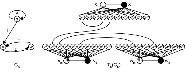
         For every vertex $v\in V_{S}$, we define a cluster of $2t+2$ unique vertices, denoted by

         $$\text{cluster}(v)\coloneqq\{v_{in}^{1},...,v_{in}^{t},v_{out}^{1},...,v_{out}^{t},v_{center},v_{marker}\}\coloneqq\{v^{1},...,v^{2t},v_{c},v_{m}\}$$

       • •

         The vertex set $V$ of $G$ is then defined as the following disjoint union:

         $$V\coloneqq\dot{\bigcup_{v\in V_{S}}}\text{cluster}(v)$$

       • •

         For every $v\in V_{S}$, the following edges are added inside $\text{cluster}(v)$:

         • –

           An edge between $v_{c}$ and $v^{i}$ for all $1\leq i\leq 2t$

         • –

           An edge between $v_{m}$ and $v^{i}$ for all $1\leq i\leq 2t-1$

         • –

           An edge between $v^{i}$ and $v^{i+1}$ for all $1\leq i\leq 2t-1$

         • –

           An edge between $v_{c}$ and $v_{m}$

       • •

         Given $v,w\in V_{S}$ (not necessarily $v\neq w$), if $I(v,w)=\{1,s_{i}\}$ then we add the edge $(v_{out}^{i},w_{in}^{i})$.
         

       

       The idea behind the construction is that every vertex $v$ in $G_{S}$ is represented by a unique fixed size cluster where each member “plays” a very specific role. Each cluster has the exact same structure, containing four types of vertices: incoming, outgoing, center and marker.

       The incoming/outgoing vertices allow representing edges in an $S$-graph that attain some value. For example, an edge between $v_{i}^{out}$ and $w_{i}^{in}$ represents an edge in $G_{S}$ between $v$ and $w$ that attains the value $I(v,w)=s_{i}$. The center vertex is used to identify which vertices belong to a single cluster, and the marker vertex is used to distinguish between $v^{1}$ and $v^{2t}$, which together with the remaining edges instills a unique order in the cluster. We denote the set of all center-type and marker-type vertices by $V_{c}$ and $V_{m}$, respectively. The set of all incoming and outgoing vertices for $s_{i}$ are denoted by $V_{in}^{i}$ and $V_{out}^{i}$, respectively. We can then write

       $$V=V_{c}\cup V_{m}\cup\bigcup_{1\leq i\leq t}V_{in}^{i}\cup\bigcup_{1\leq i\leq t}V_{out}^{i}=V_{c}\cup V_{m}\cup\bigcup_{1\leq i\leq 2t}V^{i}$$

       We claim that $T_{S}$ is well defined, and give some of its basic properties in the following lemma.

       Lemma 1.2.2.

       Let $G\coloneqq T_{S}(G_{S})\coloneqq(V,E)$ be the transformation graph of $G_{S}=(V_{S},I)$, then

       1. 1.

          $G$ is well defined.

       2. 2.

          $\forall i\hskip 11.74988pt|V^{i}|=|V_{c}|=|V_{m}|=|V_{S}|=\frac{1}{2t+2}|V|$

       3. 3.

          Let $v\in V_{S}$. Then $\deg_{G}(v_{c})=2t+1$, $\deg_{G}(v_{m})=2t$ and $\forall i\hskip 11.74988pt\deg_{G}(v^{i})<2t$. In particular the maximal degree of $G$ is exactly $2t+1$.

       4. 4.

          If $v,w\in V$ have the same $2$-disc, then they are of the same vertex type ($V^{i}/V_{c}/V_{m}$)

       Proof

       1. 1.

          By definition, the vertex set $V$ is well defined, containing exactly $|V_{S}|$ disjoint clusters of vertices, each of size $2t+2$. The only part of the construction which needs careful observation is the definition of inter-cluster edges. Given an edge $I(v,w)=\{1,s_{i}\}$ in $G_{S}$, we wish to add the edge $(v_{out}^{i},w_{in}^{i})$. This is only valid if $i\leq t$, which is of course true as $i\leq|S|<\max\{\lceil\frac{d}{2}\rceil+3,|S|+1\}=t$. In the special case $v=w$, edges from a vertex to itself correspond to the edge $(v_{out}^{i},v_{in}^{i})$. We also have the edge $(v_{in}^{t},v_{out}^{1})$, which is not an inter-cluster edge, but $|S|<t$ and so there can’t be inter-cluster edges that connect to $v_{in}^{t}$.

       2. 2.

          Each vertex in $V_{S}$ is converted to unique $2t+2$ vertices and so $|V_{S}|=\frac{1}{2t+2}|V|$. Each cluster has exactly $2t+2$ vertex types and therefore $\forall i\hskip 11.74988pt|V^{i}|=|V_{c}|=|V_{m}|=\frac{1}{2t+2}|V|$.

       3. 3.

          Let $v\in V_{S}$ be a vertex. We examine each case separately:

          • •

            The center and marker vertices $v_{c}$ and $v_{m}$ are part of a fixed amount of edges inside the cluster, and therefore ${\deg_{G}(v_{c})=2t+1}$, $\deg_{G}(v_{m})=2t$.

          • •

            If we look at $v_{in}^{i}$ ($1\leq i\leq t$), then there are at most $d$ edges between $v_{in}^{i}$ and vertices in other clusters (as the maximum amount of incoming edges of $v$ in $G_{S}$ is $d$). Inside the cluster, $v_{in}^{i}$ is connected to at most $4$ vertices: $v_{c},v_{m},v_{in}^{i-1},v_{in}^{i+1}$. Overall:

            $$\deg(v_{in}^{i})\leq d+4=2\left(\frac{d}{2}+2\right)\leq 2\left(\left(t-3\right)+2\right)=2t-2<2t$$

          • •

            The same reasoning works for $v_{out}^{i}$ ($1\leq i\leq t$).

       4. 4.

          Suppose $w,x\in V$ are two different vertices with the same $2$-disc. In particular, $\deg(w)=\deg(x)$. By the previous item, if $\deg(w)=2t+1$ or $\deg(w)=2t$ then both vertices are in $V_{c}$ or $V_{m}$, accordingly. Otherwise, we know that there are $i,j$ such that $w$ and $x$ are in $V^{i}$ and in $V^{j}$, respectively.
          If we look at the $2$-disc of $w$, then it must have exactly one neighbor with degree $2t+1$, which is the center vertex of the cluster of $w$ (an inter cluster edge will connect $w$ to a vertex in a different cluster whose degree is less than $2t$). Moreover, $w$ has at most one neighbor with degree $2t$, which is the marker vertex of its cluster. The center and marker vertices together define exactly the order of the other $2t$ vertices in the cluster (the marker distinguishes the vertex $v^{1}$ from $v^{2t}$ and then each $v^{i}$ defines $v^{i+1}$). Overall, the entire cluster of $w$ is in it’s $2$-disc and so the path $w\to v_{c}\to v^{1}\to v^{2}\to...\to w$ uniquely defines the location of $w$ in the cluster. As the $2$-discs of $w,x$ are the same, this path must be the same, and so $i=j$.
          
          

       Next, we claim that the distance between two center-type vertices in the transformation graph is at least $3$. In other words, their $1$-discs do not intersect.

       Lemma 1.2.3.

       Let $G_{S}=(V_{S},I)$ be an $S$-graph, and let $v,w\in V_{S}$ be two different vertices. Denote the graph $T_{S}(G_{S})$ by $G$. Then

       1. 1.

          If $v,w$ are adjacent then $\text{dist}_{G}(v_{c},w_{c})=3$

       2. 2.

          If $v,w$ are not adjacent then $\text{dist}_{G}(v_{c},w_{c})>3$

       In particular, $\text{disc}_{1}(v_{c})\cap\text{disc}_{1}(w_{c})=\emptyset$.

       Proof The $1$-discs of $v_{c}$ and $w_{c}$ in $G$ are both clusters of $2t+2$ vertices, which are disjoint by definition. The only edges between the clusters are those that connect in-type and out-type vertices (and not the center-type vertices), and therefore $\text{dist}_{G}(v_{c},w_{c})\geq 3$. Equality is reached only if an in-type vertex of $v$ and an out-type vertex of $w$ are connected (or the opposite), which is equivalent to saying that $v,w$ are adjacent.
       

       Having established basic properties of the transformation, we want to connect the local structures of $G_{S}$ and $G$. We know that each edge $(v,w)$ with value $s$ in $G_{S}$ corresponds to the path $v_{c}\to v_{out}^{s}\to w_{in}^{s}\to w_{c}$ in $G$, and so we might hope that the $3k$-discs of center-type vertices in $G$ might be similar to their $k$-disc counterparts in $G_{S}$.

   11. item 1.31.3

       The Projection Set $P_{q}(\Gamma_{S})$

       Suppose $v,w\in V_{S}$ are vertices with the same $k$-disc $\Gamma_{S}=\text{disc}_{k}(v)=\text{disc}_{k}(w)$. It is not necessarily true that $\text{disc}_{3k}(v_{c})=\text{disc}_{3k}(w_{c})$, as the $3k$-discs in the transformation graph may contain more than just the center-type vertices that correspond to the $k$-discs in $G$. However, the $3k$-discs are essentially the same if we think about the underlying $k$-discs that they represent. To formalize this idea, we define the projection set of a $k$-disc.

       Definition 1.3.1.

       Let $\Gamma_{S}\in\mathcal{L}_{S}(d,k)$. The $q$-projection set $P_{q}(\Gamma_{S})$ of $\Gamma_{S}$ is defined by

       $$P_{q}(\Gamma_{S})\coloneqq\bigcup_{G_{S}=(V_{S},I)\in A}\left\{\text{disc}_{q}(v_{c})|v\in V_{S},\hskip 11.74988pt\text{disc}_{k}(v)=\Gamma_{S}\right\}$$

       We denote by $P_{q}\left(\mathcal{L}_{S}(d,k)\right)$ the set of all $q$-projections

       $$P_{q}\left(\mathcal{L}_{S}(d,k)\right)\coloneqq\bigcup_{\Gamma_{S}\in\mathcal{L}_{S}(d,k)}P_{q}(\Gamma_{S})$$

       By 11.2 $(3)$ we know that the maximum degree of transformation graphs is exactly $2t+1$ and therefore $P_{q}(\Gamma_{S}),P_{q}\left(\mathcal{L}_{S}(d,k)\right)\subseteq\mathcal{L}(2t+1,q)$. The set $\mathcal{L}(2t+1,q)$ is finite (1) and so $P_{q}(\Gamma_{S}),P_{q}\left(\mathcal{L}_{S}(d,k)\right)$ are finite as well. We claim that $P_{q}\left(\mathcal{L}_{S}(d,k)\right)$ is in fact a disjoint union.

       Lemma 1.3.2.

       Let $\Gamma\in P_{q}\left(\mathcal{L}_{S}(d,k)\right)$, then there is exactly one $\Gamma_{S}$ such that $\Gamma\in P_{q}(\Gamma_{S})$.

       In particular $P_{q}\left(\mathcal{L}_{S}(d,k)\right)$ can be written as the disjoint union

       $$P_{q}\left(\mathcal{L}_{S}(d,k)\right)=\dot{\bigcup_{\Gamma_{S}\in\mathcal{L}_{S}(d,k)}}P_{q}(\Gamma_{S})$$

       Proof Let $\Gamma\in P_{q}\left(\mathcal{L}_{S}(d,k)\right)$ be a $q$-disc. By definition, there is an $S$-graph $G_{S}=(V_{S},I)$ and a vertex $v\in V_{S}$ such that $\text{disc}_{q}(v_{c})=\Gamma$ in $G\coloneqq T_{S}(G_{S})$. We can “reconstruct” $\text{disc}_{k}(v)$ from $\text{disc}_{q}(v_{c})$ with the following deterministic algorithm:

       Algorithm

       1. 1.

          function ReconstructKDisc($\Gamma=(V_{\Gamma},E_{\Gamma})$)

       2. 2.

          $V_{disc}\leftarrow\{v\}$

       3. 3.

          Init the information function $I_{disc}$ on $V_{disc}$ with $I_{disc}(v,v)=0$

       4. 4.

          for $i$ in $[k]$ do

       5. 5.

          $V_{disc}^{i}=V_{disc}$

       6. 6.

          for $w,z$ in $V_{disc}\times V_{\Gamma}$ do

       7. 7.

          if $\text{dist}(w_{c},z_{c})=3$ then

       8. 8.

          $V_{disc}^{i}=V_{disc}^{i}\cup\{z\}$

       9. 9.

          end if

       10. 10.

           end for

       11. 11.

           $V_{disc}=V_{disc}^{i}$

       12. 12.

           for $w,z,j$ in $V_{disc}\times V_{disc}\times[t]$ do

       13. 13.

           if $(w_{c},w_{out}^{j}),(w_{out}^{j},z_{in}^{j}),(z_{in}^{j},z_{c})\in E_{\Gamma}$ then

       14. 14.

           $I_{disc}(w,z)=s_{j}$

       15. 15.

           end if

       16. 16.

           end for

       17. 17.

           end for

       18. 18.

           return $G_{disc}\coloneqq(V_{disc},I_{disc})$

       19. 19.

           end function

       The algorithm starts with only the vertex $v$. In each iteration of the main for-loop (line $4$), the algorithm performs two steps:

       1. 1.

          Add any vertex $z\in V_{S}$ such that $\text{dist}(w_{c},z_{c})=3$ for some $w\in V_{S}$. By 11.2, we know that this condition is equivalent to saying that $w,z$ are adjacent in $G_{S}$. In other words, this part of the algorithm adds all vertices in $V_{S}$ that are adjacent to vertices in $V_{disc}$.

       2. 2.

          Set $I_{disc}(w,z)=s_{j}$ for any pair of vertices $w,z\in V_{disc}$ with $(w_{c},w_{out}^{j}),(w_{out}^{j},z_{in}^{j}),(z_{in}^{j},z_{c})\in E_{\Gamma}$. In other words, this part of the algorithm adds all the edges between vertices in $V_{disc}$ from the original graph $G_{S}$.

       Overall, after the $i$-th iteration of the algorithm, $(V_{disc},I_{disc})$ is exactly the $i$-disc of $v$. In particular after all $k$ iterations the algorithm returns the entire $k$-disc.
       
       We observe that the algorithm does not depend on the graph $G$ that we have chosen (we only use $G$ to prove the correctness of the algorithm), and therefore the $k$-disc of $v$ is uniquely derived from $\Gamma$. In other words, there is exactly one $\Gamma_{S}$ (the output of the algorithm) such that $\Gamma\in P_{q}(\Gamma_{S})$, as required. ∎
       

       One can think of the projection set as the set of all $q$-discs in $\mathcal{L}(2t+1,q)$ that represent the same $k$-disc in $G_{S}$, enclosed by a single definition. In the next lemma we show how this definition provides a way to connect the local structures of an $S$-graph and its transformation.

       Lemma 1.3.3.

       Let $G_{S}=(V_{S},I)$ be an $S$-graph and let $G\coloneqq T_{S}(G_{S})\coloneqq(V,E)$ be the transformation graph. Then

       1. 1.

          Let $w\in V$. Then

          $$\text{disc}_{q}(w)\in P_{q}\left(\mathcal{L}_{S}(d,k)\right)\iff w\in V_{c}$$

       2. 2.

          The sum of frequencies of $q$-discs in the projection set is given by

          $$\sum_{\Gamma\in P_{q}\left(\mathcal{L}_{S}(d,k)\right)}\text{freq}_{q}(G,\Gamma)=\frac{1}{2t+2}$$

       3. 3.

          Given $\Gamma_{S}\in\mathcal{L}_{S}(d,k)$ and a vertex $v\in V_{S}$,

          $$\text{disc}_{k}(v)=\Gamma_{S}\iff\text{disc}_{q}(v_{c})\in P_{q}(\Gamma_{S})$$

       4. 4.

          Given $\Gamma_{S}\in\mathcal{L}_{S}(d,k)$, the following holds for the counting vectors

          $$\text{cnt}_{k}(G_{S},\Gamma_{S})=\sum_{\Gamma\in P_{q}(\Gamma_{S})}\text{cnt}_{q}(G,\Gamma)$$

       5. 5.

          Given $\Gamma_{S}\in\mathcal{L}_{S}(d,k)$, the following holds for the frequency distribution vectors

          $$\text{freq}_{k}(G_{S},\Gamma_{S})=(2t+2)\cdot\sum_{\Gamma\in P_{q}(\Gamma_{S})}\text{freq}_{q}(G,\Gamma)$$

       6. 6.

          Let $H_{S}\in\Omega(S)$ be an $S$-graph, and let $H\coloneqq T_{S}(H_{S})$ be its transformation graph, then

          $$||\text{freq}_{k}(H_{S})-\text{freq}_{k}(G_{S})||_{1}\leq(2t+2)\cdot||\text{freq}_{q}(H)-\text{freq}_{q}(G)||_{1}$$

       Proof

       1. 1.

          By definition, $P_{q}\left(\mathcal{L}_{S}(d,k)\right)$ contains all possible $q$-discs of center-type vertices. If $\text{disc}_{q}(w)\in P_{q}\left(\mathcal{L}_{S}(d,k)\right)$ then it has the same $2$-disc ($2\leq q$) as some center-type vertex, and by 11.2 $(4)$ we know that $w$ is center-type itself, thus $w\in V_{c}$.

       2. 2.

          By the previous item, we know that any vertex with a $q$-disc in $P_{q}\left(\mathcal{L}_{S}(d,k)\right)$ is a center-type vertex. Therefore

          	$\displaystyle\sum_{\Gamma\in P_{q}\left(\mathcal{L}_{S}(d,k)\right)}\text{freq}_{q}(G,\Gamma)$	$\displaystyle=\frac{1}{|G|}\sum_{\Gamma\in P_{q}\left(\mathcal{L}_{S}(d,k)\right)}\text{cnt}_{q}(G,\Gamma)=\frac{1}{|G|}\sum_{\Gamma\in P_{q}\left(\mathcal{L}_{S}(d,k)\right)}|\{v\in V|\text{disc}_{q}(v)=\Gamma\}|$
          		$\displaystyle=\frac{1}{|G|}\cdot|\{v_{c}|v_{c}\in V\}|=\frac{1}{|G|}\cdot|V_{c}|=$

          Using 11.2 $(2)$, we get

          $$=\frac{1}{|G|}\cdot\frac{|G|}{2t+2}=\frac{1}{2t+2}$$

       3. 3.

          The key observation here is that $\text{disc}_{q}(v_{c})\in P(\text{disc}_{k}(v))$ (by the definition of the projection set). Thus:

          • •

            If $\text{disc}_{k}(v)=\Gamma_{S}$, then $\text{disc}_{q}(v_{c})\in P(\text{disc}_{k}(v))=P_{q}(\Gamma_{S})$

          • •

            If $\text{disc}_{q}(v_{c})\in P_{q}(\Gamma_{S})$, then $\text{disc}_{q}(v_{c})\in P(\text{disc}_{k}(v))\cap P_{q}(\Gamma_{S})$. By 11.3 we get $\text{disc}_{k}(v)=\Gamma_{S}$.

       4. 4.

          By the previous item, we have

          	$\displaystyle\text{cnt}_{k}(G_{S},\Gamma_{S})$	$\displaystyle=|\{v\in V_{S}|\text{disc}_{k}(v)=\Gamma_{S}\}|=|\{v\in V_{S}|\text{disc}_{q}(v_{c})\in P_{q}(\Gamma_{S})\}|=$
          		$\displaystyle=|\{v_{c}\in V_{c}|\text{disc}_{q}(v_{c})\in P_{q}(\Gamma_{S})\}|=$

          By the first item in this lemma, we know that only center-type vertices can have $q$-discs in $P_{q}\left(\mathcal{L}_{S}(d,k)\right)$, and therefore

          $$=|\{v\in V|\text{disc}_{q}(v_{c})\in P_{q}(\Gamma_{S})\}|=\sum_{\Gamma\in P_{q}(\Gamma_{S})}\text{cnt}_{q}(G,\Gamma)$$

       5. 5.

          Using the previous item and 11.2 $(2)$, we get

          $$\text{freq}_{k}(G_{S},\Gamma_{S})=\frac{\text{cnt}_{k}(G_{S},\Gamma_{S})}{|V_{S}|}=\frac{\sum_{\Gamma\in P_{q}(\Gamma_{S})}\text{cnt}_{q}(G,\Gamma)}{\frac{|V|}{2t+2}}=(2t+2)\cdot\sum_{\Gamma\in P_{q}(\Gamma_{S})}\text{freq}_{q}(G,\Gamma)$$

       6. 6.

          Using the previous item we have

          	$\displaystyle||\text{freq}_{k}(H_{S})-\text{freq}_{k}(G_{S})||_{1}$	$\displaystyle=\sum_{\Gamma_{S}\in\mathcal{L}_{S}(d,k)}|\text{freq}_{k}(H_{S},\Gamma_{S})-\text{freq}_{k}(G_{S},\Gamma_{S})|=$
          		$\displaystyle=(2t+2)\sum_{\Gamma_{S}\in\mathcal{L}_{S}(d,k)}|\sum_{\Gamma\in P_{q}(\Gamma_{S})}\text{freq}_{q}(H,\Gamma)-\sum_{\Gamma\in P_{q}(\Gamma_{S})}\text{freq}_{q}(G,\Gamma)|\leq$
          		$\displaystyle\leq(2t+2)\sum_{\Gamma_{S}\in\mathcal{L}_{S}(d,k)}\sum_{\Gamma\in P_{q}(\Gamma_{S})}|\text{freq}_{q}(H,\Gamma)-\text{freq}_{q}(G,\Gamma)|\leq$

          The double sum goes over all $\Gamma\in P_{q}(\Gamma_{S})$ with $\Gamma_{S}\in\mathcal{L}_{S}(d,k)$. We know by 11.3 that all projection sets are disjoint, and so each $\Gamma\in\mathcal{L}(2t+1,q)$ appears at most once, we can therefore upper bound the double sum with the entire set $\mathcal{L}(2t+1,q)$

          $$\leq(2t+2)\sum_{\Gamma\in\mathcal{L}(2t+1,q)}|\text{freq}_{q}(H,\Gamma)-\text{freq}_{q}(G,\Gamma)|=(2t+2)\cdot||\text{freq}_{q}(H)-\text{freq}_{q}(G)||_{1}$$

   12. item 1.41.4

       The Projection Subgraph

       We can look at the set $Im(T_{S})$, which contains all the simple graphs which are transformations of $S$-graphs. An arbitrary simple graph is not necessarily in $Im(T_{S})$, but it always contains a subgraph which does belong to $Im(T_{S})$ (for example, the empty subgraph). In this section, we define the projection subgraph of a simple graph and prove that it belongs to $Im(T_{S})$. We start with the definition.

       Definition 1.4.1.

       Let $G=(V,E)$ be a simple graph. We define the $q-$projection subgraph $\Psi_{q}(G)$ of $G$ as the induced subgraph of $G$ on the vertices

       $$V\left(\Psi_{q}(G)\right)\coloneqq\bigcup_{v\in V,\text{disc}_{q}(v)\in P_{q}\left(\mathcal{L}_{S}(d,k)\right)}\text{disc}_{1}(v)$$

       The idea behind the definition is that vertices in $G$ that have $q$-discs in $P_{q}\left(\mathcal{L}_{S}(d,k)\right)$ are center-type vertices. The $1$-disc of a center-type vertex is exactly its cluster, and so the union of all those clusters should be in $Im(T_{S})$. We prove this formally in the following lemma.

       Lemma 1.4.2.

       Let $G=(V,E)$ be a simple graph with maximum degree $2t+1$. Then

       1. 1.

          The union that defines the vertex set $V(\Psi_{q}(G))$ is disjoint. Namely

          $$V(\Psi_{q}(G))=\dot{\bigcup_{v\in V,\text{disc}_{q}(v)\in P_{q}\left(\mathcal{L}_{S}(d,k)\right)}}\text{disc}_{1}(v)$$

       2. 2.

          The projection subgraph is in the image of $T_{S}$

          $$\Psi_{q}(G)\in Im(T_{S})$$

          
          

       Proof Let $v,w\in V$ be two different vertices with $\text{disc}_{q}(v),\text{disc}_{q}(w)\in P_{q}\left(\mathcal{L}_{S}(d,k)\right)$. By definition, there are $S$-graphs $G_{S},H_{S}$ (possibly $G_{S}=H_{S}$) and vertices $x\in V(G_{S}),y\in V(H_{S})$ such that $\text{disc}_{q}(v)=\text{disc}_{q}(x_{c})$ and $\text{disc}_{q}(w)=\text{disc}_{q}(y_{c})$. The vertices $x_{c},y_{c}$ are center-type in $G_{S},H_{S}$ with degree $2t+1$, and therefore

       $$\text{deg}_{G}(v)=\text{deg}_{G}(w)=2t+1$$

       Suppose that $\text{disc}_{1}(v)\cap\text{disc}_{1}(w)\neq\emptyset$ and in particular $w\in\text{disc}_{2}(v)$. By $\text{disc}_{q}(v)=\text{disc}_{q}(x_{c})$, we deduce that $\text{disc}_{2}(x_{c})$ contains a vertex $z\neq x_{c}$ with $\deg_{T_{S}(G_{S})}z=2t+1$ (as ${2<3k+1=q}$). By 11.2 $(3)$, we know that $z$ is center-type. Moreover, by 11.2 we know that the distance between two center-type vertices in $T_{S}(G_{S})$ is at least $3$, which means $\text{dist}_{T_{S}(G_{S})}(x_{c},z)\geq 3$, in contradiction to $z\in\text{disc}_{2}(x_{c})$.

       In other words, the $1$-discs of $v,w$ are disjoint, and each such $1$-disc corresponds to the $1$-disc of a center-type vertex in a transformation graph. These clusters can only be interpreted in a single way, as the $2$-disc of a vertex uniquely defines its type (11.2 $(4)$). We can therefore write

       $$V(\text{disc}_{1}(v))=\{v_{in}^{1},...,v_{in}^{t},v_{out}^{1},...,v_{out}^{t},v_{c},v_{m}\}=\{v^{1},...,v^{2t},v_{c},v_{m}\}$$

       $$V(\text{disc}_{1}(w))=\{w_{in}^{1},...,w_{in}^{t},w_{out}^{1},...,w_{out}^{t},w_{c},w_{m}\}=\{w^{1},...,w^{2t},w_{c},w_{m}\}$$

       Next, we claim that an edge between two clusters must be of the form $(v_{in}^{i},w_{out}^{i})$ or $(v_{out}^{i},w_{in}^{i})$ for some $i$. The vertices $v_{c},v_{m},w_{c},w_{m}$ cannot be part of inter-cluster edges, as their counterparts in $G_{S},H_{S}$ have no inter-cluster edges. Now, suppose $e=(v^{i},w^{j})$ is an edge. In that case, $\text{disc}_{1}(w)\subseteq\text{disc}_{4}(v)$. However, $\text{disc}_{4}(v)=\text{disc}_{4}(x_{c})$ (as $q\geq 4$) and therefore the edge $e$ corresponds to some $e_{1}=(x^{i},z^{j})$ in $G_{S}$ between two clusters. In $G_{S}$, $\text{disc}_{4}(x_{c})$ contains the clusters of $x,z$ and so $e_{1}$ must be an edge of the form $(x_{in}^{i},z_{out}^{j})$ or $(x_{out}^{i},z_{in}^{j})$ for some $i$. We conclude that the edge $e$ must also be between valid end points as $\text{disc}_{4}(v)=\text{disc}_{4}(x_{c})$.

       Overall, we have shown that $V\left(\Psi_{q}(G)\right)$ is a disjoint union of clusters of size $2t+2$ that have the required ordering, and each inter-cluster edge goes from an in-vertex to an out-vertex with the same index. Therefore $\Psi_{q}(G)$ is exactly the transformation graph of some $S$-graph, which means that $\Psi_{q}(G)\in Im(T_{S})$, as required.∎
       

       Our next step is to examine the connection between the frequency vectors of $G$ and $\Psi_{q}(G)$. Informally, if $G$ is “close” to being in the image of $T_{S}$, then by 11.3 $(2)$ we would expect

       $$\sum_{\Gamma\in P_{q}\left(\mathcal{L}_{S}(d,k)\right)}\text{freq}_{q}(G,\Gamma)\approx\frac{1}{2t+2}$$

       In that case the graph $\Psi_{q}(G)$ would be very close to being all of $G$, and in particular the frequency distribution difference of the two graphs should be small. We formalize this idea in the following lemma.

       Lemma 1.4.3.

       Let $G=(V,E)$ be a simple graph with maximum degree $2t+1$. Then

       $$||\text{freq}_{q}(G)-\text{freq}_{q}(\Psi_{q}(G))||\leq\left(1+2(2t+1)^{q}\right)\left(\frac{1}{(2t+2)\sum_{\Gamma\in P_{q}\left(\mathcal{L}_{S}(d,k)\right)}\text{freq}_{q}(G,\Gamma)}-1\right)$$

       Note that if $\sum_{\Gamma\in P_{q}\left(\mathcal{L}_{S}(d,k)\right)}\text{freq}_{q}(G,\Gamma)\approx\frac{1}{2t+2}$ then the upper bound is close to $0$.
       

       Proof Using 11.4 we have

       	$\displaystyle|\Psi_{q}(G)|$	$\displaystyle=|\dot{\bigcup}_{v\in V,\text{disc}_{q}(v)\in P_{q}\left(\mathcal{L}_{S}(d,k)\right)}\text{disc}_{1}(v)|=(2t+2)|\{v\in V|\text{disc}_{q}(v)\in P\left(\mathcal{L_{S}}(d,k)\right)\}|=$
       		$\displaystyle=(2t+2)\sum_{\Gamma\in P_{q}\left(\mathcal{L}_{S}(d,k)\right)}\text{cnt}_{q}(G,\Gamma)=\left((2t+2)\sum_{\Gamma\in P_{q}\left(\mathcal{L}_{S}(d,k)\right)}\text{freq}_{q}(G,\Gamma)\right)|G|$

       We can now use 11.3 to get the required frequency difference between $G$ and its subgraph $\Psi_{q}(G)$:

       	$\displaystyle||\text{freq}_{q}(G)-\text{freq}_{q}(\Psi_{q}(G))||$	$\displaystyle\leq\frac{\left(1+2(2t+1)^{q}\right)\left(|G|-|\Psi_{q}(G)|\right)}{|\Psi_{q}(G)|}=\left(1+2(2t+1)^{q}\right)\left(\frac{|G|}{|\Psi_{q}(G)|}-1\right)$
       		$\displaystyle=\left(1+2(2t+1)^{q}\right)\left(\frac{1}{(2t+2)\sum_{\Gamma\in P_{q}\left(\mathcal{L}_{S}(d,k)\right)}\text{freq}_{q}(G,\Gamma)}-1\right)$

       This completes the proof of 11.4.∎

   13. item 1.51.5

       Reduction From S-Graphs to Simple Graphs

       In this section we prove 1.4.4. We need to show that given an arbitrarily large $S$-graph $G_{S}$ there is a fixed size $S$-graph $H_{S}$ with “similar” local structure. Our strategy is to use the assumption of the lemma to find a fixed size approximation $H$ of $T_{S}(G_{S})$ and then use the projection subgraph $\Psi_{q}(H)$ to construct a suitable $H_{S}$.
       

       Proof of 1.4.4 Let $d\geq 2,k\geq 1,\epsilon\in(0,1)$. Let $S$ be an information set and let $A\subseteq\Omega(S)$ be a natural set. By the assumption of the Lemma, we know that there is a function $f$ which satisfies the required condition of 1. We define the function $f_{S,A}$ by $f_{S,A}(d,k,\epsilon)\coloneqq f(d_{1},k_{1},\epsilon_{1})$ where $d_{1}=2t+1$, $k_{1}=q$ and

       $$\epsilon_{1}=\frac{\epsilon}{4(2t+2)^{2}\left(1+2(2t+1)^{q}\right)}$$

       Let $G_{S}=(V_{S},I)\in A$ be an $S$-graph. We need to prove that there exists an $S$-graph $H_{S}\in A$ such that

       (4)

       $$||\text{freq}_{k}(G_{S})-\text{freq}_{k}(H_{S})||_{1}\leq\epsilon\hskip 11.74988pt\wedge\hskip 11.74988pt|V(H_{S})|\leq f_{S,A}(d,k,\epsilon)$$

       We start by looking at $G\coloneqq T_{S}(G_{S})$. By 11.2, this is a well defined simple graph with maximal degree $d_{1}=2t+1$. By the definition of $f$, we know that there exists a small simple graph $H$ with

       (5)

       $$||\text{freq}_{q}(G)-\text{freq}_{q}(H)||_{1}\leq\epsilon_{1}\hskip 11.74988pt\wedge\hskip 11.74988pt|V(H)|\leq f(d_{1},k_{1},\epsilon_{1})$$

       Using 11.3 $(2)$ for $G$, we have the following lower bound for $H$:

       	$\displaystyle\sum_{\Gamma\in P_{q}\left(\mathcal{L}_{S}(d,k)\right)}\text{freq}_{q}(H,\Gamma)$	$\displaystyle=\sum_{\Gamma\in P_{q}\left(\mathcal{L}_{S}(d,k)\right)}\text{freq}_{q}(G,\Gamma)+\sum_{\Gamma\in P_{q}\left(\mathcal{L}_{S}(d,k)\right)}\left(\text{freq}_{q}(H,\Gamma)-\text{freq}_{q}(G,\Gamma)\right)\geq$
       		$\displaystyle\geq\frac{1}{2t+2}-\sum_{\Gamma\in P_{q}\left(\mathcal{L}_{S}(d,k)\right)}|\text{freq}_{q}(H,\Gamma)-\text{freq}_{q}(G,\Gamma)|\geq$
       		$\displaystyle\geq\frac{1}{2t+2}-\sum_{\Gamma\in\mathcal{L}(2t+1,q)}|\text{freq}_{q}(H,\Gamma)-\text{freq}_{q}(G,\Gamma)|=$
       		$\displaystyle=\frac{1}{2t+2}-||\text{freq}_{q}(G)-\text{freq}_{q}(H)||_{1}\geq\frac{1}{2t+2}-\epsilon_{1}$

       Using the above bound, by 11.4 we can bound the frequency difference between $H$ and $\Psi_{q}(H)$:

       (6)		$\displaystyle||\text{freq}_{q}(H)-\text{freq}_{q}(\Psi_{q}(H))||$	$\displaystyle\leq\left(1+2(2t+1)^{q}\right)\left(\frac{1}{(2t+2)\sum_{\Gamma\in P_{q}\left(\mathcal{L}_{S}(d,k)\right)}\text{freq}_{q}(G,\Gamma)}-1\right)\leq$
       	$\displaystyle\leq$	$\displaystyle\left(1+2(2t+1)^{q}\right)\left(\frac{1}{1-(2t+2)\epsilon_{1}}-1\right)$

       Next, we know by 11.4 that $\Psi_{q}(H)\in Im(T_{S})$ and so there is an $S$-graph $H_{S}^{1}$ such that $T_{S}(H_{S}^{1})=\Psi_{q}(H)$. Finally, we know that $A$ is natural, and therefore there exists an $S$-graph $H_{S}\in A$ with

       (7)

       $$||\text{freq}_{k}(G_{S})-\text{freq}_{k}(H_{S})||_{1}\leq||\text{freq}_{k}(G_{S})-\text{freq}_{k}(H_{S}^{1})||_{1}\wedge|V(H_{S})|\leq|V(H_{S}^{1})|$$

       We claim that this $H_{S}$ satisfies 4. The size requirement follows from 5, 7 and 11.2 $(2)$

       $\displaystyle|V(H_{S})|$

       $\displaystyle\leq|V(H_{S}^{1})|\leq|V(T_{S}(H_{S}^{1}))|=|V(\Psi_{q}(H))|\leq|V(H)|\leq f(d_{1},k_{1},\epsilon_{1})$

       The frequency difference follows from 6, 7 and 11.3 $(6)$

       	$\displaystyle||\text{freq}_{k}(G_{S})-\text{freq}_{k}(H_{S})||_{1}$	$\displaystyle\leq||\text{freq}_{k}(G_{S})-\text{freq}_{k}(H_{S}^{1})||_{1}\leq(2t+2)\cdot||\text{freq}_{q}(T_{S}(G_{S}))-\text{freq}_{q}(T_{S}(H_{S}^{1}))||_{1}=$
       		$\displaystyle=(2t+2)\cdot||\text{freq}_{q}(G)-\text{freq}_{q}(\Psi_{q}(H))||_{1}\leq$
       		$\displaystyle\leq(2t+2)\cdot\left(||\text{freq}_{q}(G)-\text{freq}_{q}(H)||_{1}+||\text{freq}_{q}(H)-\text{freq}_{q}(\Psi_{q}(H))||_{1}\right)\leq$
       		$\displaystyle\leq(2t+2)\cdot\left(\epsilon_{1}+\left(1+2(2t+1)^{q}\right)\left(\frac{1}{1-(2t+2)\epsilon_{1}}-1\right)\right)\leq\epsilon$

       The last inequality is technical and does not depend on $G$. The proof to that inequality is given in 11.4.

       Overall, we have shown that for any arbitrary $G_{S}\in A$ there is an $S$-graph $H_{S}^{1}\in A$ of size at most ${f_{S,A}(d,k,\epsilon)=f(d_{1},k_{1},\epsilon_{1})}$, with a local structure that approximates the local structure of $G_{S}$. In other words, $f_{S,A}$ satisfies the condition on 11.4. This completes the proof of 1.4.4. ∎

   14. item 1.61.6

       Proof of Winkler’s Theorem for Simple Graphs

       In this section we will use the transformation $T_{S}$ and the tools that we have developed in the previous sections to prove the simple variant of Winkler’s theorem (11.2). We will prove this theorem by constructing a reduction from the directed edge-colored variant. Together with the reduction from PCP to the directed edge-colored variant (11.1), this creates a reduction from PCP to the simple variant of Winkler’s question. If we compare this to Alon’s question, then the interreducibility theorem is the “second” step and what remains is to show how PCP can be reduced to the directed edge-colored variant. Before we can prove the theorem, we need a generalized version of the projection set, where we also consider $q$-discs of non center-type vertices.

       Definition 1.6.1.

       Let $d\geq 2,k\geq 1$. We define the generalized $q-$projection set by

       $$\widetilde{P_{q}}\coloneqq\bigcup_{G_{S}=(V_{S},I)\in A}\left\{\text{disc}_{q}(v)|v\in V(T_{S}(G_{S}))\right\}$$

       The set $\widetilde{P_{q}}$ contains all the possible $q$-discs of vertices in $T_{S}(G_{S})$, including those of non center-type vertices. In particular $P_{q}\left(\mathcal{L}_{S}(d,k)\right)\subseteq\widetilde{P_{q}}$. We claim that if the $q$-disc set of a simple graph $G$ is contained in the generalized $q$-projection set, then the $q$-projection subgraph $\Psi_{q}(G)$ is the entire graph.

       Lemma 1.6.2.

       Let $G=(V,E)$ be a simple graph with $\{\text{disc}_{q}(v)|v\in V(G)\}\subseteq\widetilde{P_{q}}$. Then $G=\Psi_{q}(G)$.

       Proof The projection subgraph $\Psi_{q}(G)$ is by definition a subgraph of $G$, so we only need to prove that any vertex $v\in G$ also belongs to $\Psi_{q}(G)$. To this end, let $v\in G$. By the assumption on $G$, we know that $\text{disc}_{q}(v)\in\widetilde{P_{q}}$. This means that there is a graph $H_{S}$, and a vertex $w\in V(T_{S}(H_{S}))$ with

       (8)

       $$\text{disc}_{q}(v)=\text{disc}_{q}(w)$$

       By the definition of $T_{S}$, there is a vertex $w_{S}\in V(H_{S})$ such that $w\in cluster(w_{S})$. Thus, $w$ is either a center-type vertex, or connected by an edge to a center-type vertex. In both cases, $w$ belongs to the $1$-disc of some vertex with degree $2t+1$ (by 11.2 $(3)$). Using 8, we deduce that in $G$, the vertex $v$ is also in the $1$-disc of a vertex with degree $2t+1$. Denote that vertex by $z$ (possibly $z=v$). Once again, by 11.2 $(3)$ we know that the $q$-disc of $z$ must correspond to a center-type vertex in some $S$-graph and therefore $z\in\Psi_{q}(G)$. In particular $v\in\text{disc}_{1}(z)\in\Psi_{q}(G)$, which is what we had to prove.∎
       

       The following is an immediate corollary of 11.6 and 11.4 $(2)$.

       Corollary 1.6.3.

       Let $G=(V,E)$ be a simple graph with $\{\text{disc}_{q}(v)|v\in V(G)\}\subseteq\widetilde{P_{q}}$. Then $G\in Im(T_{S})$.

       We now have all the perquisites required to prove the main theorem of this section.
       

       Proof of 11.2 We prove the theorem by reduction from the problem for directed edge colored graphs (i.e. $S$-graphs) to the simple variant. To this end, let $\Phi_{S}$ be a set of $S$-graphs, and assume that the simple problem is decidable, say by an algorithm $Alg=Alg(d,k,\Phi)$. We will construct a deterministic algorithm $AlgDC$ which uses $Alg$ as a subroutine to decide the directed edge-colored variant of Winkler’s problem. The main idea of the proof is that asking the directed edge-colored question for $\Phi_{S}$ is similar to asking the simple question for the set

       $$\Phi\coloneqq\bigcup_{\Gamma_{S}\in\Phi_{S}}P_{q}(\Gamma_{S})\subseteq P_{q}\left(\mathcal{L}_{S}(d,k)\right)$$

       If $G_{S}$ is a $S$-graph whose $k$-disc set is $\Phi_{S}$, then $T_{S}(G_{S})$ will also have $q$-discs of non center-type vertices. To overcome this problem, we use the generalized projection set $\widetilde{P_{q}}$. We now give the implementation of $AlgDC$.

       Algorithm

       1. 1.

          function AlgDC($d,k,\Phi_{S}=\{\Gamma_{S}^{1},...,\Gamma_{S}^{n}\}$)

       2. 2.

          Construct the sets $\widetilde{P_{q}}$ and $\forall i\ P_{q}(\Gamma_{S}^{i})$.

       3. 3.

          for every $\emptyset\neq X_{i}\subseteq P_{q}(\Gamma_{S}^{i})$ and $Y\subseteq\widetilde{P_{q}}\backslash P_{q}\left(\mathcal{L}_{S}(d,k)\right)$ do

       4. 4.

          if $Alg(t,q,\bigcup_{i=1}^{n}X_{i}\cup Y)$ is “True” then

       5. 5.

          return “True”

       6. 6.

          end if

       7. 7.

          end for

       8. 8.

          return “False”

       9. 9.

          end function

       We start by explaining why the algorithm is deterministic. To construct the sets $P_{q}(\Gamma_{S}^{i})$ and $\widetilde{P_{q}}$, we theoretically need to go over all $S$-graphs, which cannot be done in finite time. However, by 11.2 we know that any $q$-disc in $P_{q}(\Gamma_{S}^{i})$ can have at most $2d^{q}$ vertices, and in particular it can have vertices of at most $2d^{q}$ clusters in the transformation graph. This means that it is enough to examine transformation graphs with at most $2d^{q}$ clusters, or equivalently, it is enough to examine $S$-graphs of size at most $\frac{1}{2t+2}2d^{q}$ (by 11.2 $(2)$). The for-loop runs over all possible choices of suitable $X_{i}$ and $Y$. There is only a finite amount of such choices, as $P_{q}(\Gamma_{S}^{i})$ and $\widetilde{P_{q}}$ are finite. In each iteration, the algorithm calls $Alg$, which is deterministic by assumption, and therefore the entire loop runs in finite time. We conclude that the entire algorithm is deterministic, as required.
       It remains to prove that the algorithm returns “True” if and only if there is an $S$-graph $G_{S}$ with

       $$\{\text{disc}_{k}(v)|v\in V(G_{S})\}=\varPhi_{S}$$

       For the first direction, assume that there is a graph $G_{S}=(V_{S},I)$ with the $k$-disc set $\Phi_{S}=\{\Gamma_{S}^{1},...,\Gamma_{S}^{n}\}$. If we look at the graph $G\coloneqq T_{S}(G_{S})$, then by definition

       		$\displaystyle\{\text{disc}_{q}(v)|v\in V(G)\}=\left(\bigcup_{i=1}^{n}\left\{\text{disc}_{q}(v_{c})|v\in V_{S},\>\text{disc}_{k}(v)=\Gamma_{S}^{i}\right\}\right)\cup\{\text{disc}_{q}(v)|v\in V(G),v\notin V_{c}\}\subseteq$
       		$\displaystyle\subseteq\bigcup_{i=1}^{n}P_{q}(\Gamma_{S}^{i})\cup\left(\widetilde{P_{q}}\backslash P_{q}\left(\mathcal{L}_{S}(d,k)\right)\right)$

       Where the last inclusion is based on the fact that non center-type vertices cannot have a $q$-disc in $P_{q}\left(\mathcal{L}_{S}(d,k)\right)$ (as even their $2$-discs differ by 11.2 $(4)$) . We know by the assumption on $G_{S}$ that for any $i$ the set $X_{i}=\left\{\text{disc}_{q}(v_{c})|v\in V_{S},\>\text{disc}_{k}(v)=\Gamma_{S}^{i}\right\}$ is not empty and so this union contains non empty subsets of $P_{q}(\Gamma_{S}^{i})$. All the remaining $q$-discs in $G$ form a subset $Y$ of $\widetilde{P_{q}}\backslash P_{q}\left(\mathcal{L}_{S}(d,k)\right)$. We have thus found sets $\emptyset\neq X_{i}\subseteq P_{q}(\Gamma_{S}^{i})$ and $Y\subseteq\widetilde{P_{q}}\backslash P_{q}\left(\mathcal{L}_{S}(d,k)\right)$ such that $\{\text{disc}_{q}(v)|v\in V(G)\}=\bigcup_{i=1}^{n}X_{i}\cup Y$. In particular, the for-loop iteration that considers this choice of $X_{i}$ and $Y$ will return “True”.
       

       For the second direction, assume that the algorithm returned “True”. Then, there are sets $\{X_{i}\}_{i=1}^{n}$ and $Y$ with $\emptyset\neq X_{i}\subseteq P_{q}(\Gamma_{S}^{i})$ and $Y\subseteq\widetilde{P_{q}}\backslash P_{q}\left(\mathcal{L}_{S}(d,k)\right)$ for which $Alg(t,q,\bigcup_{i=1}^{n}X_{i}\cup Y)$ returned “True”. By the definition of $Alg$, this means that there is a simple graph $G$ with $\{\text{disc}_{q}(v)|v\in V(G)\}=\bigcup_{i=1}^{n}X_{i}\cup Y$ and in particular

       $$\{\text{disc}_{q}(v)|v\in V(G)\}=\bigcup_{i=1}^{n}X_{i}\cup Y\subseteq\left(\bigcup_{i=1}^{n}P_{q}(\Gamma_{S}^{i})\right)\cup\left(\widetilde{P_{q}}\backslash P_{q}\left(\mathcal{L}_{S}(d,k)\right)\right)\subseteq\widetilde{P_{q}}$$

       Note that this is the required condition of 11.6, from which we deduce that $G\in Im(T_{S})$. In other words, there is an $S$-graph $G_{S}$ such that $T_{S}(G_{S})=G$. We claim that the $k$-disc set of $G_{S}$ is exactly $\varPhi_{S}$, namely

       $$\{\text{disc}_{k}(v)|v\in V(G_{S})\}=\varPhi_{S}$$

       We prove this equality by double inclusion.

       1. 1.

          Let $v\in V(G_{S})$, we claim that $\text{disc}_{k}(v)\in\varPhi_{S}$.
          We look at the $q$-disc $\text{disc}_{q}(v_{c})$ of the center-type vertex corresponding to $v$ in $G$. By the definition of the $q$-projection set, we know that

          $$\text{disc}_{q}(v_{c})\in P_{q}(\text{disc}_{k}(v))\subseteq P_{q}\left(\mathcal{L}_{S}(d,k)\right)$$

          We also know that $\text{disc}_{q}(v_{c})\in\{\text{disc}_{q}(v)|v\in V(G)\}=\bigcup_{i=1}^{n}X_{i}\cup Y$, but $Y\subseteq\widetilde{P_{q}}\backslash P_{q}\left(\mathcal{L}_{S}(d,k)\right)$ and so there is some index $i$ such that

          $$\text{disc}_{q}(v_{c})\in X_{i}\subseteq P_{q}(\Gamma_{S}^{i})$$

          We conclude that $\text{disc}_{q}(v_{c})\in P_{q}(\text{disc}_{k}(v))\cap P_{q}(\Gamma_{S}^{i})$, and so by 11.3 we get $\text{disc}_{k}(v)=\Gamma_{S}^{i}$. By definition, $\Gamma_{S}^{i}\in\varPhi_{S}$ and so $\text{disc}_{k}(v)\in\varPhi_{S}$.

       2. 2.

          Let $1\leq i\leq n$. We claim that there is a vertex $v\in V(G_{S})$ such that $\text{disc}_{k}(v)=\Gamma_{S}^{i}$.
          By the definition of $G$, there is a center-type vertex $v_{c}\in G$ with $\text{disc}_{q}(v_{c})\in X_{i}\subseteq P_{q}(\Gamma_{S}^{i})$. If we look at the vertex $v\in V(G_{S})$ to which $v_{c}$ corresponds, then by definition $\text{disc}_{q}(v_{c})\in P_{q}(\text{disc}_{k}(v))$. We therefore have $\text{disc}_{q}(v_{c})\in P_{q}(\text{disc}_{k}(v))\cap P_{q}(\Gamma_{S}^{i})$ and so again by 11.3 we conclude that $\text{disc}_{k}(v)=\Gamma_{S}^{i}$.
          

       To conclude, we have shown that the deterministic algorithm $AlgDC(d,k,\varPhi_{S})$, which uses $Alg$ as a subroutine, returns “True” if and only if there is a $S$-graph $G_{S}$ with $\{\text{disc}_{k}(v)|v\in V(G_{S})\}=\varPhi_{S}$. This is, of course, a contradiction to 11.1. Therefore the assumption is wrong, and there is no deterministic algorithm that solves the simple variant of Winkler’s problem, as required.∎
   15. item 1.11.1

       Local Structure of Paths

       In the previous chapters we have examined the question of finding a small graph that approximates the local structure of an arbitrary large graph. The interreducibility theorem shows that any model which is a natural extension of the simple model does not change the difficulty of that question. We have conjectured that there is a reduction from PCP to our main question (11.2). One can think of a solution to a PCP system as a single long string, constructed by concatenating the PCP tiles. This long string can be thought of as an $S$-graph of a path, where each edge contains a letter or a set of letters which comprise the string. It is therefore interesting to ask what happens if we restrict our problem to approximating arbitrary long paths by paths of bounded size. In this chapter, we will look at different ways to define the “local structure” of a path, and prove that in all cases the problem of finding a small approximating path is decidable.

   16. item 1.21.2

       Undirected Paths

       Before we examine the general case, we note that the problem of approximating an undirected path with a small undirected path is trivial. This is because the local structure of a path on $n$ vertices is uniquely defined.

       Fact 1.2.1.

       Let $k\geq 1,\epsilon\in(0,1)$, and let $P$ be an undirected path. Then there is an undirected path $Q$ such that

       $$||\text{freq}_{k}(P)-\text{freq}_{k}(Q)||_{1}\leq\epsilon\hskip 11.74988pt\wedge\hskip 11.74988pt|V(Q)|\leq\lfloor\frac{4k}{\epsilon}\rfloor+1$$

       Proof An undirected path has a very simple local structure. There are exactly $k$ vertices on each side of the path with $k$-discs that include the “boundary” of the path, while all the rest have the same $k$-disc $\Gamma$ which is a path of length $2k$. If we assume that $|P|,|Q|>2k$ then

       	$\displaystyle||\text{freq}_{k}(P)-\text{freq}_{k}(Q)||_{1}$	$\displaystyle=\sum_{\Delta\in\mathcal{L}(d,k)}|\text{freq}_{k}(P,\Delta)-\text{freq}_{k}(Q,\Delta)|=2k|\frac{1}{|P|}-\frac{1}{|Q|}|+|\text{freq}_{k}(P,\Gamma)-\text{freq}_{k}(Q,\Gamma)|=$
       		$\displaystyle=2k|\frac{1}{|P|}-\frac{1}{|Q|}|+|\frac{|P|-2k}{|P|}-\frac{|Q|-2k}{|Q|}|=4k|\frac{1}{|Q|}-\frac{1}{|P|}|$

       If $|P|\leq\lfloor\frac{4k}{\epsilon}\rfloor+1$ then taking $Q=P$ is sufficient. Otherwise we take $Q$ to be the path of length $\lfloor\frac{4k}{\epsilon}+1\rfloor$ and then

       $$||\text{freq}_{k}(P)-\text{freq}_{k}(Q)||_{1}=4k|\frac{1}{|Q|}-\frac{1}{|P|}|=4k\left(\frac{1}{|Q|}-\frac{1}{|P|}\right)\leq\frac{4k}{|Q|}=\frac{4k}{\lfloor\frac{4k}{\epsilon}\rfloor+1}\leq\frac{4k}{\frac{4k}{\epsilon}}=\epsilon$$

       As required.∎

   17. item 1.31.3

       S-Paths and S-Cycles

       The general question for directed edge-colored paths is not as trivial as the undirected case. When we say “directed edge-colored path” we mean that the path graph can be written as a sequence $v_{1},...,v_{n}$ where the only edges in the path are $\forall i\ (v_{i},v_{i+1})$ and each edge attains some value $s\in S$. We start by defining this formally.

       Definition 1.3.1.

       Let $S$ be a finite information set (can represent colors, strings, letters etc).

       Let $n\in\mathbb{N}$ and let $V=\{v_{1},...,v_{n}\}$ be a set of vertices. Let $G=(V,I)\in\Omega(S)$ be an $S$-graph.

       Suppose the following holds for some $x\in\{0\}\cup\left\{\{1\}\times S\right\}$:

       $$\forall v,w\in V\hskip 11.74988ptI(v,w)=\begin{cases}(1,s_{i})&\exists i\hskip 11.74988ptv=v_{i},w=v_{i+1}\\ x&v=v_{n},w=v_{1}\\ 0&\text{otherwise}\end{cases}$$

       If $x=0$, we say that $G$ is an $S$-path. Otherwise, we say that $G$ is an $S$-cycle. In both cases, we say that the size of $G$ is $|V_{S}|=n$.

       Let $k\geq 1$ be an integer, and let $G=(V,I)$ be an $S$-path/$S$-cycle. The $k$-disc of a vertex $v\in V$ is defined similarly as in the general $S$-graph model. In addition, if $2k+2\leq|G|$ then the $k$-disc of every vertex is itself an $S$-path. Just like in the original problem, two $k$-discs are said to be isomorphic if and only if there is a root preserving isomorphism which also preserves $I$. We claim that under these definitions, the problem of finding a small $S$-path that approximates an arbitrary $S$-path is decidable.

       Theorem 1.3.2.

       Let $k\geq 1,\epsilon\in(0,1)$. Let $P$ be a $S$-path, then there is an $S$-path $Q$ such that

       $$||\text{freq}_{k}(P)-\text{freq}_{k}(Q)||_{1}\leq\epsilon\ \wedge\ |Q|\leq\frac{24960d^{3k}|S|^{2}L_{S}^{6}(d,k)}{\epsilon^{2}}$$

       The proof is based on the following two lemmas, which will be proven in the next sections of this chapter.

       Lemma 1.3.3.

       Let $k\geq 1,\epsilon\in(0,1)$. Let $G\in\Omega(S)$ be a disjoint union of $S$-cycles, each of size at least $2k+2$. Then, there is an $S$-graph $H\in\Omega(S)$ which is a disjoint union of $S$-cycles and $S$-paths such that

       $$||\text{freq}_{k}(G)-\text{freq}_{k}(H)||_{1}\leq\epsilon\ \wedge\ |H|\leq\frac{130d^{k}|S|^{2}L_{S}^{5}(d,k)}{\epsilon}$$

       Lemma 1.3.4.

       Let $k\geq 1,\epsilon\in(0,1)$. Let $G\in\Omega(S)$ be an $S$-graph which is a disjoint union of $S$-cycles, each of size at least $2k+2$. Then there is an $S$-path $P$ such that

       $$||\text{freq}_{k}(G)-\text{freq}_{k}(P)||_{1}\leq\epsilon\ \wedge\ |P|\leq\frac{8d^{k}L_{S}(d,k)}{\epsilon}|G|$$

       Having stated the lemmas, we are now ready to prove the main theorem of this chapter.
       

       Proof of 11.2 \ 11.3

       Let $k\geq 1,\epsilon\in(0,1)$, and let $P=(V,I)$ be an $S$-path. We need to find an $S$-path $Q$ such that

       $$||\text{freq}_{k}(P)-\text{freq}_{k}(Q)||_{1}\leq\epsilon\ \wedge\ |Q|\leq\varphi$$

       Where

       $$\varphi=\frac{24960d^{3k}|S|^{2}L_{S}^{6}(d,k)}{\epsilon^{2}}$$

       We can assume that $\varphi<|P|$ (otherwise taking $Q=P$ is sufficient), and in particular

       $$|P|\geq\max\{2k+2,\frac{12d^{k}L_{S}(d,k)}{\epsilon}\}$$

       Denote the set of vertices of $P$ by $V(P)=\{v_{1},...,v_{n}\}$, and let $s\in S$ be a value. We start by defining the cycle $C$ which is formed by adding the edge $I(v_{n},v_{1})=s$ to $P$. By 11.3, we know that

       $$||\text{freq}_{k}(P)-\text{freq}_{k}(C)||_{1}\leq\frac{4d^{k}L_{S}(d,k)}{|P|}\leq\frac{\epsilon}{3}$$

       We know that $2k+2<|P|=|C|$, and so in particular $C$ is a disjoint union of $S$-cycles, each of size at least $2k+2$. By 11.3, we know that there is an $S$-graph $H$ which is a disjoint union of $S$-cycles and $S$-paths such that

       $$||\text{freq}_{k}(C)-\text{freq}_{k}(H)||_{1}\leq\frac{\epsilon}{24d^{k}}\leq\frac{\epsilon}{6}\ \wedge\ |H|\leq\frac{3120d^{2k}|S|^{2}L_{S}^{5}(d,k)}{\epsilon}$$

       Denote the disjoint components of $H$ by $H_{1}^{C},...,H_{n_{1}}^{C}$ and $H_{1}^{P},...,H_{n_{2}}^{P}$ which are cycles and paths, respectively. We define a new graph $\widetilde{H}$, in one of the two following ways:

       1. 1.

          If $\sum_{i=1}^{n_{2}}|H_{i}^{P}|<2k+2$, we set $\widetilde{H}$ to be just the components $H_{1}^{C},...,H_{n_{1}}^{C}$. Each of the vertices in $H_{1}^{P},...,H_{n_{2}}^{P}$ has a $k$-disc which does not appear in $C$ (it is either an $S$-cycle or a small $S$-path), and therefore

          $$\frac{\sum_{i=1}^{n_{2}}|H_{i}^{P}|}{|H|}\leq\sum_{\Gamma\in\mathcal{L}_{S}(d,k)}|\text{freq}_{k}(C,\Gamma)-\text{freq}_{k}(H,\Gamma)|\leq\frac{\epsilon}{24d^{k}}$$

          We then have

          $\displaystyle|H|-\sum_{i=1}^{n_{2}}|H_{i}^{P}|$

          $\displaystyle\geq\frac{24d^{k}\sum_{i=1}^{n_{2}}|H_{i}^{P}|}{\epsilon}-\sum_{i=1}^{n_{2}}|H_{i}^{P}|\geq\frac{6(1+2d^{k})\sum_{i=1}^{n_{2}}|H_{i}^{P}|}{\epsilon}$

          We use this bound, together with 11.3 to get

          $\displaystyle||\text{freq}_{k}(\widetilde{H})-\text{freq}_{k}(H)||_{1}$

          $\displaystyle\leq\frac{(1+2d^{k})\left(|H|-|\widetilde{H}|\right)}{|\widetilde{H}|}=\frac{(1+2d^{k})\sum_{i=1}^{n_{2}}|H_{i}^{P}|}{|H|-\sum_{i=1}^{n_{2}}|H_{i}^{P}|}\leq\frac{\epsilon(1+2d^{k})\sum_{i=1}^{n_{2}}|H_{i}^{P}|}{6(1+2d^{k})\sum_{i=1}^{n_{2}}|H_{i}^{P}|}=\frac{\epsilon}{6}$

       2. 2.

          If $2k+2\leq\sum_{i=1}^{n_{2}}|H_{i}^{P}|$, we set $\widetilde{H}$ to be just components $H_{1}^{C},...,H_{n_{1}}^{C}$ and also add one addition component $H^{P}$ which is a concatenation of $H_{1}^{P},...,H_{n_{2}}^{P}$ into a single $S$-cycle where all the new edges get some arbitrary value $s\in S$). We claim that $\widetilde{H}$ is a better approximation of $C$ than $H$, as a result of the weight-shifting lemma (11.3). Indeed, let $\Gamma\in\mathcal{L}(d,k)$ be a $k$-disc with $\text{freq}_{k}(\widetilde{H},\Gamma)<\text{freq}_{k}(H,\Gamma)$. The only vertices in $H$ whose $k$-disc has changed are those who were edges in $S$-paths, and so the only $k$-discs whose frequency decreases are those which are not full $S-$paths of length $2k+1$. There are no such vertices in $C$ (as it is a disjoint union of $S$-cycles), and therefore $\text{freq}_{k}(C,\Gamma)=0$. By the weight-shifting lemma, we then have

          $$||\text{freq}_{k}(\widetilde{H})-\text{freq}_{k}(C)||_{1}\leq||\text{freq}_{k}(H)-\text{freq}_{k}(C)||_{1}\leq\frac{\epsilon}{24d^{k}}\leq\frac{\epsilon}{6}$$

       Overall, we have constructed a graph $\widetilde{H}$ which is a disjoint union of $S$-cycles of size at least $2k+2$. We then have by the triangle inequality

       $$||\text{freq}_{k}(\widetilde{H})-\text{freq}_{k}(C)||_{1}\leq||\text{freq}_{k}(\widetilde{H})-\text{freq}_{k}(H)||_{1}+||\text{freq}_{k}(H)-\text{freq}_{k}(C)||_{1}\leq\frac{\epsilon}{6}+\frac{\epsilon}{6}\leq\frac{\epsilon}{3}$$

       Finally, by 11.3, we know that there there is an $S$-path $Q$ such that

       $$||\text{freq}_{k}(\widetilde{H})-\text{freq}_{k}(Q)||_{1}\leq\frac{\epsilon}{3}\ \wedge\ |Q|\leq\frac{8d^{k}L_{S}(d,k)}{\epsilon}|\widetilde{H}|$$

       We claim that this $S$-path $Q$ satisfies the needed requirements. By the triangle inequality we know that the local structure of $Q$ is close to the local structure of $P$

       		$\displaystyle||\text{freq}_{k}(P)-\text{freq}_{k}(Q)||_{1}\leq$
       		$\displaystyle\leq||\text{freq}_{k}(P)-\text{freq}_{k}(C)||_{1}+||\text{freq}_{k}(C)-\text{freq}_{k}(\widetilde{H})||_{1}+||\text{freq}_{k}(\widetilde{H})-\text{freq}_{k}(Q)||_{1}\leq$
       		$\displaystyle\leq\frac{\epsilon}{3}+\frac{\epsilon}{3}+\frac{\epsilon}{3}=\epsilon$

       And we also know that $Q$ is small

       $$|Q|\leq\frac{8d^{k}L_{S}(d,k)}{\epsilon}|\widetilde{H}|\leq\frac{8d^{k}L_{S}(d,k)}{\epsilon}\cdot\frac{3120d^{2k}|S|^{2}L_{S}^{5}(d,k)}{\epsilon}=\frac{24960d^{3k}|S|^{2}L_{S}^{6}(d,k)}{\epsilon^{2}}$$

       We can plug in $d=2$ and use the naive bound $L_{S}(d,k)=L_{S}(2,k)\leq(2k)^{|S|}$ (a $k$-disc of an $S$-path can have at most $2k-1$ directional edges that attain values in $S$) to get the bound

       $$|Q|\leq 24960\frac{8^{k}|S|^{2}(2k)^{6|S|}}{\epsilon^{2}}$$

       Which is an explicit bound only depending on $d,k,|S|$. This completes the proof of the theorem.∎
       
       In conclusion, we have shown that for any $\epsilon>0$ and any $S$-path $P$, it is possible to find a small $S$-path $Q$, whose size does not depend on $P$ such that

       $$||\text{freq}_{k}(P)-\text{freq}_{k}(Q)||_{1}\leq\epsilon$$

       This means that the question of finding a small approximation is decidable for $S$-paths, and in particular it is not possible to construct a reduction from PCP to this variant of the problem.
   18. item 1.41.4

       Rewiring Edges In S-Cycles

       In this section we prove 11.3 by utilizing the “rewire and split” technique, which was also used to prove 11.1. The lemma claims that an arbitrary $S$-graph $G$ which is a disjoint union of $S$-cycles can be approximated by a “small” $S$-graph $H$ which is a disjoint union of $S$-cycles and $S$-paths. We start by defining some additional graph related notation that will be used in this section.
       

       Let $G=(V,I)$ be an $S$-graph. Given a subset $W\subseteq V$ of vertices, we denote by $\text{cnt}_{k}(W|G)$ the relative $k$-disc count vector whose entries only count the number of $k$-discs of each type attained by vertices in $W$. The relative $k$-disc frequency distribution vector is defined by $\text{freq}_{k}(W|G)=\text{cnt}_{k}(W|G)/|W|$. If $\Gamma\in\mathcal{L}_{S}(d,k)$ is a $k$-disc then $\text{cnt}_{k}(W|G,\Gamma)$ and $\text{freq}_{k}(W|G,\Gamma)$ denote the entries in the relative vectors which correspond to $\Gamma$.

       Suppose that $V_{1}\dot{\cup}V_{2}=V$ is a partitioning of $V$ into two disjoint subsets. We define the set of all directional edges from $V_{1}$ to $V_{2}$ by $e_{G}(V_{1},V_{2})\coloneqq|\{(x,y)|x\in V_{1},y\in V_{2},\ I(x,y)\neq 0\}|$.

       The cut of the partition is defined by

       $$\text{cut}_{G}(V_{1},V_{2})=e_{G}(V_{1},V_{2})+e_{G}(V_{2},V_{1})$$

       Next, we define the measure $\alpha$ of the partition:

       $$\alpha\coloneqq\alpha_{G}(V_{1},V_{2})\coloneqq\max_{\Gamma\in\mathcal{L}_{S}(d,k)}|\text{freq}_{k}(V_{1}|G,\Gamma)-\text{freq}_{k}(V_{2}|G,\Gamma)|$$

       The function $\alpha$ measures how “balanced” is the partition in terms of local structure. If the local structures of $V_{1},V_{2}$ are close, then $\alpha$ would be close to $0$. Finally, we define the value $e_{s}(P_{1},P_{2}|X,Y)$.

       Definition 1.4.1.

       Let $G=(V,I)$ be a disjoint union of $S$-cycles, and let $X,Y\subseteq V$ be two subsets of $V$ (not necessarily disjoint). Given some value $s\in S$ and two $S$-paths $P_{1},P_{2}$ of size $k$, we denote by $e_{s}(P_{1},P_{2}|X,Y)$ the amount of $S$-paths $P=\{p_{1},...,p_{2k}\}$ in $G$ of size $2k$ where:

       1. 1.

          The subgraphs induced by $\{p_{1},...,p_{k}\}$ and $\{p_{k+1},...,p_{2k}\}$ are isomorphic to $P_{1}$ and $P_{2}$, respectively.

       2. 2.

          The vertices $p_{k}$ and $p_{k+1}$ are in $X$ and $Y$, respectively, with $I(p_{k},p_{k+1})=s$

       In other words, $e_{s}(P_{1},P_{2}|X,Y)$ counts the amount of edges in $G$ that connect the two $S$-paths ($P_{1}$ and $P_{2}$) by an edge from $X$ to $Y$ with the value $s$.
       

       Our first lemma gives a basic connection between the measure $\alpha$ and the value $e_{s}(P_{1},P_{2}|X,Y)$.

       Lemma 1.4.2.

       Let $k\geq 1$. Let $G=(V,I)$ be a disjoint union of $S$-cycles, each of size at least $2k+2$, and let $V_{1}\dot{\cup}V_{2}=V$ be a partitioning of $V$. Let $s\in S$ and let $P_{1},P_{2}$ be $S$-paths of size $k$, then

       $$|\frac{e_{s}(P_{1},P_{2}|V_{1},V)}{|V_{1}|}-\frac{e_{s}(P_{1},P_{2}|V_{2},V)}{|V_{2}|}|,|\frac{e_{s}(P_{1},P_{2}|V,V_{1})}{|V_{1}|}-\frac{e_{s}(P_{1},P_{2}|V,V_{2})}{|V_{2}|}|\leq\alpha_{G}(V_{1},V_{2})|S|$$

       Proof Suppose that $e=(x,y)$ is an edge from $x$ to $y$ that is counted by $e_{s}(P_{1},P_{2}|V_{1},V)$ or $e_{s}(P_{1},P_{2}|V_{2},V)$. Since $x$ belongs to a cycle of size at least $2k+2$, we know that the $k$-disc of $x$ is an $S$-path of size $2k+1$ of the form $X(t_{1})=t_{1}P_{1}sP_{2}$ for some $t_{1}\in S$. Summing over all possible $t_{1}$ we get

       $$e_{s}(P_{1},P_{2}|V_{1},V)=\sum_{t_{1}\in S}\text{cnt}_{k}(V_{1}|G,X(t_{1}))\hskip 11.74988pte_{s}(P_{1},P_{2}|V_{2},V)=\sum_{t_{1}\in S}\text{cnt}_{k}(V_{2}|G,X(t_{1}))$$

       We then have

       	$\displaystyle|\frac{e_{s}(P_{1},P_{2}|V_{1},V)}{|V_{1}|}-\frac{e_{s}(P_{1},P_{2}|V_{2},V)}{|V_{2}|}|$	$\displaystyle=|\frac{\sum_{t_{1}\in S}\text{cnt}_{k}(V_{1}|G,X(t_{1}))}{|V_{1}|}-\frac{\sum_{t_{1}\in S}\text{cnt}_{k}(V_{2}|G,X(t_{1}))}{|V_{2}|}|=$
       		$\displaystyle=|\sum_{t_{1}\in S}\text{freq}_{k}(V_{1}|G,X(t_{1}))-\sum_{t_{1}\in S}\text{freq}_{k}(V_{2}|G,X(t_{1}))$
       		$\displaystyle\leq\sum_{t_{1}\in S}|\text{freq}_{k}(V_{1}|G,X(t_{1}))-\text{freq}_{k}(V_{2}|G,X(t_{1}))|\leq\alpha_{G}(V_{1},V_{2})|S|$

       Similarly, if $e=(x,y)$ is an edge from $x$ to $y$ that is counted by $e_{s}(P_{1},P_{2}|V,V_{1})$ or $e_{s}(P_{1},P_{2}|V,V_{2})$, then the $k$-disc of $y$ is an $S$-path of size $2k+1$ of the form $P_{1}sP_{2}t_{1}$ for some $t_{1}\in S$. Similar analysis gives us

       $$|\frac{e_{s}(P_{1},P_{2}|V,V_{1})}{|V_{1}|}-\frac{e_{s}(P_{1},P_{2}|V,V_{2})}{|V_{2}|}|\leq\alpha_{G}(V_{1},V_{2})|S|$$

       This completes the proof of 11.4.∎
       

       We proceed by using the above lemma to give a better connection between the measures.

       Lemma 1.4.3.

       Let $k\geq 1$. Let $G=(V,I)$ be a disjoint union of $S$-cycles, each of size at least $2k+2$, and let $V_{1}\dot{\cup}V_{2}=V$ be a partitioning of $V$. Let $s\in S$ and let $P_{1},P_{2}$ be $S$-paths of size $k$, then

       $$|e_{s}(P_{1},P_{2}|V_{1},V_{2})-e_{s}(P_{1},P_{2}|V_{2},V_{1})|\leq 2\frac{|V_{1}||V_{2}|}{|V|}\alpha_{G}(V_{1},V_{2})|S|$$

       Proof Since $V_{1}\dot{\cup}V_{2}=V$ is a disjoint partition, we have the following identities for $i\in\{1,2\}$

       $$e_{s}(P_{1},P_{2}|V_{i},V)=e_{s}(P_{1},P_{2}|V_{i},V_{1})+e_{s}(P_{1},P_{2}|V_{i},V_{2})$$

       $$e_{s}(P_{1},P_{2}|V,V_{i})=e_{s}(P_{1},P_{2}|V_{1},V_{i})+e_{s}(P_{1},P_{2}|V_{2},V_{i})$$

       We use these identities to get an upper bound on the required difference

       		$\displaystyle|e_{s}(P_{1},P_{2}|V_{1},V_{2})-e_{s}(P_{1},P_{2}|V_{2},V_{1})|=$
       		$\displaystyle=\frac{|V_{1}||V_{2}|}{|V|}\cdot\frac{|V_{1}|+|V_{2}|}{|V_{1}||V_{2}|}|e_{s}(P_{1},P_{2}|V_{1},V_{2})-e_{s}(P_{1},P_{2}|V_{2},V_{1})|$
       		$\displaystyle=\frac{|V_{1}||V_{2}|}{|V|}\cdot|\left(\frac{1}{|V_{1}|}+\frac{1}{|V_{2}|}\right)\left(e_{s}(P_{1},P_{2}|V_{1},V_{2})-e_{s}(P_{1},P_{2}|V_{2},V_{1})\right)+0-0|$
       		$\displaystyle=\frac{|V_{1}||V_{2}|}{|V|}\cdot|\left(\frac{1}{|V_{1}|}+\frac{1}{|V_{2}|}\right)\left(e_{s}(P_{1},P_{2}|V_{1},V_{2})-e_{s}(P_{1},P_{2}|V_{2},V_{1})\right)+$
       		$\displaystyle+\frac{e_{s}(P_{1},P_{2}|V_{1},V_{1})-e_{s}(P_{1},P_{2}|V_{1},V_{1})}{|V_{1}|}-\frac{e_{s}(P_{1},P_{2}|V_{2},V_{2})-e_{s}(P_{1},P_{2}|V_{2},V_{2})}{|V_{2}|}|=$
       		$\displaystyle=\frac{|V_{1}||V_{2}|}{|V|}\cdot|\frac{e_{s}(P_{1},P_{2}|V_{1},V_{2})}{|V_{1}|}+\frac{e_{s}(P_{1},P_{2}|V_{1},V_{2})}{|V_{2}|}-\frac{e_{s}(P_{1},P_{2}|V_{2},V_{1})}{|V_{1}|}-\frac{e_{s}(P_{1},P_{2}|V_{2},V_{1})}{|V_{2}|}+$
       		$\displaystyle+\frac{e_{s}(P_{1},P_{2}|V_{1},V_{1})-e_{s}(P_{1},P_{2}|V_{1},V_{1})}{|V_{1}|}-\frac{e_{s}(P_{1},P_{2}V_{2},V_{2})-e_{s}(P_{1},P_{2}|V_{2},V_{2})}{|V_{2}|}|=$
       		$\displaystyle=\frac{|V_{1}||V_{2}|}{|V|}\cdot|\frac{e_{s}(P_{1},P_{2}|V_{1},V_{2})+e_{s}(P_{1},P_{2}|V_{1},V_{1})}{|V_{1}|}+\frac{e_{s}(P_{1},P_{2}|V_{1},V_{2})+e_{s}(P_{1},P_{2}|V_{2},V_{2})}{|V_{2}|}$
       		$\displaystyle-\frac{e_{s}(P_{1},P_{2}|V_{2},V_{1})+e_{s}(P_{1},P_{2}|V_{1},V_{1})}{|V_{1}|}-\frac{e_{s}(P_{1},P_{2}|V_{2},V_{1})+e_{s}(P_{1},P_{2}|V_{2},V_{2})}{|V_{2}|}|$
       		$\displaystyle=\frac{|V_{1}||V_{2}|}{|V|}\cdot|\frac{e_{s}(P_{1},P_{2}|V_{1},V)}{|V_{1}|}+\frac{e_{s}(P_{1},P_{2}|V,V_{2})}{|V_{2}|}-\frac{e_{s}(P_{1},P_{2}|V,V_{1})}{|V_{1}|}-\frac{e_{s}(P_{1},P_{2}|V_{2},V)}{|V_{2}|}|\leq$
       		$\displaystyle\leq\frac{|V_{1}||V_{2}|}{|V|}\cdot\left(|\frac{e_{s}(P_{1},P_{2}|V_{1},V)}{|V_{1}|}-\frac{e_{s}(P_{1},P_{2}|V_{2},V)}{|V_{2}|}|+|\frac{e_{s}(P_{1},P_{2}|V,V_{1})}{|V_{1}|}-\frac{e_{s}(P_{1},P_{2}|V,V_{2})}{|V_{2}|}|\right)$

       Finally, by 11.4, we get

       $$|e_{s}(P_{1},P_{2}|V_{1},V_{2})-e_{s}(P_{1},P_{2}|V_{2},V_{1})|\leq\frac{|V_{1}||V_{2}|}{|V|}\cdot\left(\alpha_{G}(V_{1},V_{2})|S|+\alpha_{G}(V_{1},V_{2})|S|\right)=2\frac{|V_{1}||V_{2}|}{|V|}\alpha_{G}(V_{1},V_{2})|S|$$

       This completes the proof of 11.4.∎
       
       This result allows us to analyze our main technical tool, that is, the rewiring of edges. We will define a condition on a partition of $G$, and show that if that condition holds, the edges in $G$ can be “rewired” in a way that decreases the cut of the partition, without altering the FDVs of each part. We will also show that when the condition no longer holds, the cut between the parts must be small.

       Lemma 1.4.4.

       Let $k\geq 1,\epsilon\in(0,1)$ and let $G=(V,I_{G})$ be a disjoint union of $S$-cycles, each of size at least $2k+2$. Suppose $V_{1}\dot{\cup}V_{2}=V$ is a partitioning of $V$. Then, either there exists an $S$-graph $H=(V,I_{H})$ which is a disjoint union of $S$-cycles, each of size at least $2k+2$ such that

       (9)

       $$\forall v\in V\ \text{disc}_{k}(G,v)\cong\text{disc}_{k}(H,v)\hskip 11.74988pt\wedge\hskip 11.74988pt\text{cut}_{H}(V_{1},V_{2})=\text{cut}_{G}(V_{1},V_{2})-2$$

       or the cut of $G$ is small

       (10)

       $$\text{cut}_{G}(V_{1},V_{2})\leq|S|L_{S}^{2}(d,k)\left(8k+6+2\frac{|V_{1}||V_{2}|}{|V|}\alpha_{G}(V_{1},V_{2})|S|\right)$$

       The proof of the lemma will be based on the following condition.

       Condition 1.4.5.

       There exist two disjoint isomorphic $S$-paths of size $2k$ in $G$, denoted by $P=\{p_{1},...p_{k},p_{k+1},p_{2k}\}$ and $Q=\{q_{1},...q_{k},q_{k+1},q_{2k}\}$ such that

       (11)

       $$\text{dist}_{G}(p_{1},q_{2k}),\text{dist}_{G}(q_{1},p_{2k})\geq 3\>\wedge p_{k},q_{k+1}\in V_{1}\ \wedge q_{k},p_{k+1}\in V_{2}$$

       We claim that if the condition is satisfied, then Eq. (9) holds, and if not then Eq. (10) holds.
       

       Proof of 11.4 For the first direction, suppose there are disjoint isomorphic $S$-paths $P,Q$ of size $2k$ that satisfy 11.We define the $S$-graph $H=(V,I_{H})$ in the following way

       $$\forall v,w\in V\hskip 11.74988ptI_{H}(v,w)=\begin{cases}I_{G}(p_{k},p_{k+1})&(v,w)\in\{(p_{k},q_{k+1}),(q_{k},p_{k+1})\}\\ 0&(v,w)\in\{(p_{k},p_{k+1}),(q_{k},q_{k+1})\}\\ I_{G}(v,w)&\text{otherwise}\end{cases}$$

       In other words, we replace the edges $(p_{k},p_{k+1})$ and $(q_{k},q_{k+1})$ by $(p_{k},q_{k+1})$ and $(q_{k},p_{k+1})$. All four edges attain the same value $s\coloneqq I_{G}(p_{k},p_{k+1})$. We observe that

       $$\text{cut}_{H}(V_{1},V_{2})=\text{cut}_{G}(V_{1},V_{2})-2$$

       as we have replaced two edges between $V_{1},V_{2}$ with two edges which are contained within the sets. Next, we claim that $H$ is a disjoint union of $S$-cycles of size at least $2k+2$ and that the $k$-discs of all vertices in the graph have not changed. We distinguish between two cases:

       1. 1.

          The $S$-paths $P,Q$ are part of the same $S$-cycle $C$ in $G$.

          In this case, we can write $C=\{p_{1},...,p_{2k},x_{1},...,x_{i},q_{1},...,q_{2k},y_{1},...,y_{j}\}$. We know by 11 that $\text{dist}_{G}(p_{1},q_{2k}),\text{dist}_{G}(q_{1},p_{2k})\geq 3$ and therefore $i,j\geq 2$. After the rewiring, $C$ becomes the two disjoint cycles $C_{1}=\{p_{1},...,p_{k},q_{k+1},...,q_{2k},y_{1},...,y_{j}\}$ and $C_{2}=\{q_{1},...,q_{k},p_{k+1},...,p_{2k},x_{1},...,x_{i}\}$. We then have

          $$|C_{1}|=k+k+j\geq 2k+2\hskip 11.74988pt|C_{2}|=k+k+i\geq 2k+2$$

          Moreover, no $k$-discs have been affected, as the $k$-discs of all vertices in $C_{1},C_{2}$ are the same $S$-paths of size $2k$ as in $C$ (due to $P,Q$ being isomorphic). No other component in the graph $G$ has been affected.

       2. 2.

          The $S$-paths $P$ and $Q$ are in different $S$-cycles $C_{1}$ and $C_{2}$, respectively, in $G$.

          In this case, we can write $C_{1}=\{p_{1},...,p_{2k},y_{1},...,y_{j}\}$and $C_{2}=\{q_{1},...,q_{2k},x_{1},...,x_{i}\}$ where $i,j\geq 2$ (as the $S$-cycles in $G$ are of size at least $2k+2$). After the rewiring, the two $S$-cycles become the single $S$-cycle $C=\{p_{1},...,p_{k},q_{k+1},...,q_{2k},x_{1},...,x_{i},q_{1},...,q_{k},p_{k+1},...,p_{2k},y_{1},...,y_{j}\}$ of size $4k+i+j\geq 2k+2$. Just like the first case, no $k$-discs have changed, and no other components have been affected.

       To summarize, we have shown that if 11.4 is satisfied, then there is a graph $H$ that satisfies 9.
       

       In the other direction, suppose that 11.4 is not satisfied. Any $S$-path of length $2k$ can be written as a concatenation of two $S$-paths of size $k$, connected by an edge between them. To this end, let $s\in S$ and let $P_{1},P_{2}$ be two $S$-paths of size $k$. We look at the $S$-path $P_{1}sP_{2}$ of size $2k$, and examine the following sum

       $$e_{s}(P_{1},P_{2}|V_{1},V_{2})+e_{s}(P_{1},P_{2}|V_{2},V_{1})$$

       First Case: $e_{s}(P_{1},P_{2}|V_{1},V_{2})\neq 0$

       In this case, we know that there is an $S$-path $P$ in $G$ which is isomorphic to $P_{1}sP_{2}$.

       Suppose $e=(x,y)$ is an edge that has been counted by $e_{s}(P_{1},P_{2}|V_{2},V_{1})$. By definition, the $S$-path $Q$ of size $2k$ which is formed by taking $\text{disc}_{k}(x)\cup\text{disc}_{k}(y)$ is isomorphic to $P$. We therefore have the $S$-paths $P,Q$ which are isomorphic (as both are isomorphic to $P_{1}sP_{2}$). By our assumption, 11.4 is not satisfied and therefore $P,Q$ must either intersect or satisfy

       $$\text{dist}_{G}(p_{1},q_{2k}),\text{dist}_{G}(q_{1},p_{2k})<3$$

       If we look at the $S$-cycle $C=\{p_{1},...,p_{2k},c_{1},...,c_{i}\}$ to which $P$ belongs, then this requirement is equivalent to $q_{1}\in\{p_{1},...,p_{2k},c_{1},c_{2},c_{i-2k},...,c_{i}\}$, and in particular there are at most $2k+2+(2k+1)=4k+3$ possible ways to construct $Q$. Therefore $e_{s}(P_{1},P_{2}|V_{2},V_{1})\leq 4k+3$, and so by 11.4

       $$e_{s}(P_{1},P_{2}|V_{1},V_{2})+e_{s}(P_{1},P_{2}|V_{2},V_{1})\leq 4k+3+\left(4k+3+2\frac{|V_{1}||V_{2}|}{|V|}\alpha_{G}(V_{1},V_{2})|S|\right)$$

       Second Case: $e_{s}(P_{1},P_{2}|V_{1},V_{2})=0$

       In this case, directly from 11.4 we have

       $$e_{s}(P_{1},P_{2}|V_{1},V_{2})+e_{s}(P_{1},P_{2}|V_{2},V_{1})\leq 0+\left(0+2\frac{|V_{1}||V_{2}|}{|V|}\alpha_{G}(V_{1},V_{2})|S|\right)$$

       We conclude that for any choice of $s\in S$ and $S$-paths $P_{1},P_{2}$ of size $k$ we have

       (12)

       $$e_{s}(P_{1},P_{2}|V_{1},V_{2})+e_{s}(P_{1},P_{2}|V_{2},V_{1})\leq 8k+6+2\frac{|V_{1}||V_{2}|}{|V|}\alpha_{G}(V_{1},V_{2})|S|$$

       Finally, we know that $G$ consists of $S$-cycles of length at least $2k+2$, and so every edge in $G$ is the middle edge of exactly one $S$-path of size $2k$. We can use this observation to define the cut of the partition in terms of $s,P_{1},P_{2}$ in the following way

       $$\text{cut}_{G}(V_{1},V_{2})=e_{G}(V_{1},V_{2})+e_{G}(V_{2},V_{1})=\sum_{s,P_{1},P_{2}}\left(e_{s}(P_{1},P_{2}|V_{1},V_{2})+e_{s}(P_{1},P_{2}|V_{2},V_{1})\right)$$

       Using 12, and the fact that the amount of possible $k$-paths is bounded by $L_{S}(d,k)$ (in fact even $L_{S}(d,\frac{k}{2})$) we have

       	$\displaystyle\text{cut}_{G}(V_{1},V_{2})$	$\displaystyle=\sum_{s,P_{1},P_{2}}\left(e_{s}(P_{1},P_{2}|V_{1},V_{2})+e_{s}(P_{1},P_{2}|V_{2},V_{1})\right)=$
       		$\displaystyle\leq|S|L_{S}^{2}(d,k)\max_{s,P_{1},P_{2}}\left(e_{s}(P_{1},P_{2}|V_{1},V_{2})+e_{s}(P_{1},P_{2}|V_{2},V_{1})\right)\leq$
       		$\displaystyle\leq|S|L_{S}^{2}(d,k)\left(8k+6+2\frac{|V_{1}||V_{2}|}{|V|}\alpha_{G}(V_{1},V_{2})|S|\right)$

       This completes the proof of the second direction, and of 11.4.∎
       

       We can now finally prove 11.3. Given a disjoint union of $S$-cycles $G$, our strategy would be to define a partition of $G$ with a small $\alpha$, and then perform the edge rewiring manipulation on the graph $G$ for as long as 11.4 is satisfied. We will then use the resulting graph to find a small approximation of $G$.

       Proof of 11.3

       Let $G$ be a disjoint union of $S$-cycles of size at least $2k+2$. We need to find an $S$-graph $H$ which is a disjoint union of $S$-cycles and $S$-paths such that

       $$||\text{freq}_{k}(G)-\text{freq}_{k}(H)||_{1}\leq\epsilon\ \wedge\ |H|\leq 2\varphi$$

       Where

       $$\varphi\coloneqq\frac{65d^{k}|S|^{2}L_{S}^{5}(d,k)}{\epsilon}$$

       We can assume that $2\varphi<|G|$ (otherwise taking $H=G$ is sufficient). We start by defining the disjoint partition $V_{1}\dot{\cup}V_{2}=V$ of $G$. For each $\Gamma\in\mathcal{L}_{S}(d,k)$, we denote the set of vertices in $G$ with $k$-disc $\Gamma$ by $\{v_{\Gamma}^{1},...,v_{\Gamma}^{\text{cnt}_{k}(G,\Gamma)}\}$. We then define

       $$V_{1}=\bigcup_{\Gamma\in\mathcal{L}_{S}(d,k)}\{v_{\Gamma}^{1},...,v_{\Gamma}^{\lceil\varphi\cdot\text{freq}_{k}(G,\Gamma)\rceil}\},\hskip 11.74988ptV_{2}=V/V_{1}$$

       This partition is well defined as $\lceil\varphi\cdot\text{freq}_{k}(G,\Gamma)\rceil<\lceil|G|\cdot\text{freq}_{k}(G,\Gamma)\rceil=\text{cnt}_{k}(G,\Gamma)$. Moreover, we observe that $|V_{1}|\in\varphi\left(\varphi,\varphi+L_{S}(d,k)\right)$ as

       $$\varphi=\sum_{\Gamma\in\mathcal{L}_{S}(d,k)}\varphi\cdot\text{freq}_{k}(G,\Gamma)\leq|V_{1}|\leq\sum_{\Gamma\in\mathcal{L}_{S}(d,k)}\left(\varphi\cdot\text{freq}_{k}(G,\Gamma)+1\right)\leq\varphi+L_{S}(d,k)$$

       We can use that to also get the bound $|V_{2}|=|V|-|V_{1}|\in(|V|-\varphi-L_{S}(d,k),|V|-\varphi)$.

       Now, let $\Gamma\in\mathcal{L}_{S}(d,k)$ be a $k$-disc. We then have

       		$\displaystyle|\text{freq}_{k}(V_{1}|G,\Gamma))-\text{freq}_{k}(G,\Gamma)|=|\frac{\lceil\varphi\cdot\text{freq}_{k}(G,\Gamma)\rceil}{|V_{1}|}-\text{freq}_{k}(G,\Gamma)|\leq$
       		$\displaystyle\leq\max\{\text{freq}_{k}(G,\Gamma)-\frac{\lceil\varphi\cdot\text{freq}_{k}(G,\Gamma)\rceil}{\varphi+L_{S}(d,k)},\frac{\lceil\varphi\cdot\text{freq}_{k}(G,\Gamma)\rceil}{\varphi}-\frac{\varphi\text{freq}_{k}(G,\Gamma)}{\varphi}\}$
       		$\displaystyle\leq\max\{\frac{L_{S}(d,k)}{\varphi+L_{S}(d,k)},\frac{1}{\varphi}\}\leq\frac{L_{S}^{2}(d,k)}{\varphi}$

       And in particular, if we sum over all $\Gamma$ then

       (13)

       $$|\text{freq}_{k}(V_{1}|G))-\text{freq}_{k}(G)|\leq\frac{L_{S}^{3}(d,k)}{\varphi}$$

       
       

       Similar calculation can be done for $V_{2}$, if we also use the fact that $2\varphi<|V|$:

       		$\displaystyle|\text{freq}_{k}(G,\Gamma)-\text{freq}_{k}(V_{2}|G,\Gamma)|=$
       		$\displaystyle=|\text{freq}_{k}(G,\Gamma)-\frac{\text{cnt}_{k}(G,\Gamma)-\lceil\varphi\cdot\text{freq}_{k}(G,\Gamma)\rceil}{|V_{2}|}|=$
       		$\displaystyle=\max\{\text{freq}_{k}(G,\Gamma)-\frac{\text{cnt}_{k}(G,\Gamma)-\lceil\varphi\cdot\text{freq}_{k}(G,\Gamma)\rceil}{|V|-\varphi},\frac{\text{cnt}_{k}(G,\Gamma)-\lceil\varphi\cdot\text{freq}_{k}(G,\Gamma)\rceil}{|V|-\varphi-L_{S}(d,k)}-\text{freq}_{k}(G,\Gamma)\}$
       		$\displaystyle\leq\max\{\frac{1}{|V|-\varphi},\frac{L_{S}(d,k)}{|V|-\varphi-L_{S}(d,k)}\}\leq\max\{\frac{1}{\varphi},\frac{L_{S}(d,k)}{\varphi-L_{S}(d,k)}\}\leq\frac{L_{S}^{2}(d,k)}{\varphi}$

       By the triangle inequality, we conclude that

       $$\alpha\coloneqq\alpha_{G}(V_{1},V_{2})=\max_{\Gamma\in\mathcal{L}_{S}(d,k)}|\text{freq}_{k}(V_{1}|G,\Gamma)-\text{freq}_{k}(V_{2}|G,\Gamma)|\leq\frac{2L_{S}^{2}(d,k)}{\varphi}$$

       Now, by 11.4 we know that either

       (14)

       $$\text{cut}_{G}(V_{1},V_{2})\leq|S|L_{S}^{2}(d,k)\left(8k+6+2\frac{|V_{1}||V_{2}|}{|V|}\alpha_{G}(V_{1},V_{2})|S|\right)$$

       or the graph $G$ can be replaced with a graph $\widetilde{G}$ on the same vertex set that preserves the $k$-discs of all vertices on one side, and has exactly two edges less between $V_{1},V_{2}$. One can repeat this process at most a finite amount of times (as the amount of edges between $V_{1},V_{2}$ is finite) to finally get a graph $\widetilde{G}$ with the same $k$-discs as in $G$ which satisfies 14. In particular, we have

       (15)

       $$\text{freq}_{k}(\widetilde{G})=\text{freq}_{k}(G)\wedge\text{freq}_{k}(V_{1}|\widetilde{G})=\text{freq}_{k}(V_{1}|G)$$

       If we plug in the bounds for $|V_{1}|,|V_{2}|$ and $\alpha_{G}$, we get

       	$\displaystyle\text{cut}_{\widetilde{G}}(V_{1},V_{2})$	$\displaystyle\leq|S|L_{S}^{2}(d,k)\left(8k+6+2\frac{|V_{1}||V_{2}|}{|V|}\alpha_{G}(V_{1},V_{2})|S|\right)\leq$
       		$\displaystyle\leq|S|L_{S}^{2}(d,k)\left(8k+6+2\left(\varphi+L_{S}(d,k)\right)\frac{2L_{S}^{2}(d,k)}{\varphi}|S|\right)\leq$
       		$\displaystyle\leq|S|L_{S}^{2}(d,k)\left(8k+6+8L_{S}^{2}(d,k)|S|\right)\leq 16|S|^{2}L_{S}^{4}(d,k)$

       Finally, we define the graph $H\coloneqq\widetilde{G}[V_{1}]$ which is formed by removing all the edges between $V_{1}$ and $V_{2}$ in $\widetilde{G}$ and then taking the subgraph induced by $V_{1}$. As a subgraph of $\widetilde{G}$ (which we know to be a disjoint union of $S$-cycles), we know that $H$ is a disjoint union of $S$-cycles and $S$-paths.

       By 11.3, we have a bound on the difference between the FDVs of $H$ and $V_{1}|\widetilde{G}$

       $\displaystyle||\text{freq}_{k}(V_{1}|\widetilde{G})-\text{freq}_{k}(H)||_{1}$

       $\displaystyle\leq\frac{4d^{k}\left(\text{cut}_{\widetilde{G}}(V_{1},V_{2})\right)L_{S}(d,k)}{|V_{1}|}\leq\frac{4d^{k}\left(16|S|^{2}L_{S}^{4}(d,k)\right)L_{S}(d,k)}{|V_{1}|}\leq\frac{64d^{k}|S|^{2}L_{S}^{5}(d,k)}{\varphi}$

       Together with 13 and 15 we conclude that

       		$\displaystyle||\text{freq}_{k}(G)-\text{freq}_{k}(H)||_{1}\leq$
       		$\displaystyle\leq||\text{freq}_{k}(G)-\text{freq}_{k}(V_{1}|G))||_{1}+||\text{freq}_{k}(V_{1}|G))-\text{freq}_{k}(V_{1}|\widetilde{G})||_{1}+||\text{freq}_{k}(V_{1}|\widetilde{G})-\text{freq}_{k}(H)||_{1}\leq$
       		$\displaystyle\leq\frac{L_{S}^{3}(d,k)}{\varphi}+0+\frac{64d^{k}|S|^{2}L_{S}^{5}(d,k)}{\varphi}\leq\frac{65d^{k}|S|^{2}L_{S}^{5}(d,k)}{\varphi}=\epsilon$

       And we can also bound the size of $H$

       $$|V(H)|=|V_{1}|\leq\varphi+L_{S}(d,k)\leq 2\varphi$$

       This completes the proof of 11.3. ∎
   19. item 1.51.5

       Blowing-Up S-Cycles

       In this section we prove 11.3. The lemma states that a disjoint union of big $S$-cycles can be approximated by a single $S$-path. The idea is that if there is a small amount of cycles, and each cycle is very big (in terms of amount of vertices), then “removing” one edge from each cycle and connecting all the formed $S$-paths together creates a single $S$-path, with a very small amount of vertices whose $k$-discs have been affected.
       However, if the cycles are small, than each edge removal affects a relatively big portion of the vertices in that cycle. To handle that, we need to start by blowing up the cycles in a way that the amount of vertices drastically increases but the frequency does not change by much.

       The first lemma of this section shows how blowing up cycles of size at least $2k+2$ does not affect their frequency.

       Lemma 1.5.1.

       Let $k\geq 1$ and let $C=(V,I)$ be an $S$-cycle of size at least $2k+2$. Denote the vertices of $C$ by $V=\{v_{1},...,v_{n}\}$ (where each consecutive pair has an edge). Denote $I(v_{n},v_{1})$ by $c$.

       Let $P$ be the $S$-path formed by removing the edge $(v_{n},v_{1})$ from $C$ and let $C_{1}$ be the $S$-cycle formed by concatenating $m>0$ copies of $P$ one to another where the last vertex of a copy is connected by an edge to the first vertex in the next copy and the value of that edge is $c$. Then

       $$\text{freq}_{k}(C_{1})=\text{freq}_{k}(C)\ \wedge\ |C_{1}|=m|C|$$

       Proof By the definition of $C_{1}$, we know that $|C_{1}|=m|P|=m|C|$.

       By the way we constructed $C_{1}$, we know that each vertex in $C_{1}$ has a $k$-disc of an $S$-path which is exactly the same as its origin vertex in $C$ (as the $S$-cycles are of size at least $2k+2$). Moreover, if $\Gamma\in\mathcal{L}_{S}(d,k)$ is the $k$-disc of $t$ vertices in $V$, then there are exactly $mt$ vertices in $C_{1}$ with this $k$-disc. Therefore

       	$\displaystyle\text{freq}_{k}(C_{1})$	$\displaystyle=\sum_{\Gamma\in\mathcal{L}_{S}(d,k)}\text{freq}_{k}(C_{1},\Gamma)=\frac{1}{|C_{1}|}\sum_{\Gamma\in\mathcal{L}_{S}(d,k)}\text{cnt}_{k}(C_{1},\Gamma)=\frac{1}{m|C|}\sum_{\Gamma\in\mathcal{L}_{S}(d,k)}\left(m\cdot\text{cnt}_{k}(C,\Gamma)\right)=$
       		$\displaystyle=\sum_{\Gamma\in\mathcal{L}_{S}(d,k)}\frac{\text{cnt}_{k}(C,\Gamma)}{|C|}=\sum_{\Gamma\in\mathcal{L}_{S}(d,k)}\text{freq}_{k}(C,\Gamma)=\text{freq}_{k}(C)$

       This completes the proof of the lemma.∎
       

       We can now prove the Cycle Blowup lemma. Our strategy would be to blow up the original cycles, remove a single edge from each, and finally connect all the resulting paths into a single path.
       

       Proof of 11.3 Let $k\geq 1,\epsilon\in(0,1)$. Let $G\in\Omega(S)$ be an $S$-graph which is a disjoint union of $S$-cycles, each of size at least $2k+2$. Let $t$ be the amount of $S$-cycles in $G$. Denote this set of cycles by $C_{1},...C_{t}$. Then

       $$\text{freq}_{k}(G)=\frac{\text{cnt}_{k}(G)}{|G|}=\sum_{i=1}^{t}\frac{\text{cnt}_{k}(C_{i})}{|G|}=\sum_{i=1}^{t}\frac{|C_{i}|}{|G|}\text{freq}_{k}(C_{i})$$

       Let

       $$m=\lceil\frac{4d^{k}(2t-1)L_{S}(d,k)}{\epsilon|G|}\rceil\leq\frac{8d^{k}tL_{S}(d,k)}{\epsilon|G|}$$

       By the previous lemma, we know that each of these cycles can be “blown up” to a a cycle of size $m|C_{i}|$ such that the FDV is not changed. Denote those new large cycles by $M_{1},...,M_{t}$. We then have

       $$\forall i\hskip 11.74988pt\text{freq}_{k}(M_{i})=\text{freq}_{k}(C_{i})\ \wedge\ |M_{i}|=m|C_{i}|$$

       Now, we remove a single edge from each of those cycles, and denote the resulting paths by $P_{1},...,P_{t}$.

       By 11.3, we know that the removal only slightly altered the FDVs:

       $$\forall i\hskip 11.74988pt||\text{freq}_{k}(P_{i})-\text{freq}_{k}(M_{i})||_{1}\leq\frac{4d^{k}L_{S}(d,k)}{|M_{i}|}=\frac{4d^{k}L_{S}(d,k)}{m|C_{i}|}$$

       Let $H$ be the disjoint union of all the paths $P_{i}$, then

       $$\text{freq}_{k}(H)=\frac{\text{cnt}_{k}(H)}{|H|}=\sum_{i=1}^{t}\frac{\text{cnt}_{k}(P_{i})}{|H|}=\sum_{i=1}^{t}\frac{|P_{i}|}{|H|}\text{freq}_{k}(P_{i})$$

       And

       $$|H|=\sum_{i=1}^{t}|P_{i}|=\sum_{i=1}^{t}|M_{i}|=m\sum_{i=1}^{t}|C_{i}|=m|G|$$

       Finally, let $s\in S$ be some value. We define the $S$-path $P$ which is formed by connecting all the paths $P_{i}$, where the new edges, connecting the paths, all attain the value $s$.

       Once again by 11.3, we know that $P$ is formed by adding $t-1$ edges to $H$ and so

       $\displaystyle||\text{freq}_{k}(P)-\text{freq}_{k}(H)||_{1}$

       $\displaystyle\leq\frac{4d^{k}(t-1)L_{S}(d,k)}{|H|}=\frac{4d^{k}(t-1)L_{S}(d,k)}{m|G|}$

       We claim that $P$ satisfies the required condition. First, using the fact that $t\leq|G|$ we have

       $$|P|=|H|=m|G|\leq\left(\frac{8d^{k}tL_{S}(d,k)}{\epsilon|G|}\right)|G|=\frac{8d^{k}tL_{S}(d,k)}{\epsilon}\leq\frac{8d^{k}L_{S}(d,k)}{\epsilon}|G|$$

       And secondly, we have

       		$\displaystyle||\text{freq}_{k}(P)-\text{freq}_{k}(G)||_{1}\leq$
       		$\displaystyle\leq||\text{freq}_{k}(P)-\text{freq}_{k}(H)||_{1}+||\text{freq}_{k}(H)-\text{freq}_{k}(G)||_{1}=$
       		$\displaystyle=||\text{freq}_{k}(P)-\text{freq}_{k}(H)||_{1}+||\sum_{i=1}^{t}\frac{|P_{i}|}{|H|}\text{freq}_{k}(P_{i})-\sum_{i=1}^{t}\frac{|C_{i}|}{|G|}\text{freq}_{k}(C_{i})||_{1}=$
       		$\displaystyle=||\text{freq}_{k}(P)-\text{freq}_{k}(H)||_{1}+||\sum_{i=1}^{t}\frac{m|C_{i}|}{m|G|}\text{freq}_{k}(P_{i})-\sum_{i=1}^{t}\frac{|C_{i}|}{|G|}\text{freq}_{k}(M_{i})||_{1}\leq$
       		$\displaystyle\leq||\text{freq}_{k}(P)-\text{freq}_{k}(H)||_{1}+\sum_{i=1}^{t}\frac{|C_{i}|}{|G|}|\text{freq}_{k}(P_{i})-\text{freq}_{k}(M_{i})|\leq$
       		$\displaystyle\leq\frac{4d^{k}(t-1)L_{S}(d,k)}{m|G|}+\sum_{i=1}^{t}\frac{|C_{i}|}{|G|}\frac{4d^{k}L_{S}(d,k)}{m|C_{i}|}=$
       		$\displaystyle=\frac{4d^{k}(t-1)L_{S}(d,k)+4d^{k}tL_{S}(d,k)}{m|G|}=\frac{4d^{k}(2t-1)L_{S}(d,k)}{m|G|}\leq\epsilon$

       We have therefore constructed a path $P$ which approximated the local structure of $G$ and has the required size restriction. This completes the proof of the lemma.∎
   20. item 1.61.6

       Alternative Local Structure Definitions

       We have shown in the previous sections that under the standard definition of the cnt/freq vectors, the problem of approximating an $S$-path with a small $S$-path is decidable. Using the fact that the $k$-disc of each vertex in a long $S$-path is an $S$-path, it is possible to define the cnt/freq vectors differently, and then ask the question of finding a small approximation. For example, we can count only the left/right parts of the $k$-disc (i.e take the $S$-path that starts at a vertex without looking “backward”).
       
       In general, let $P_{k}(S)$ be the set of $k$-discs of vertices in an $S$-path, and let $M:P_{k}(S)\to X$ be a function which maps the $k$-discs to some finite set $X$. Then by 11.3 we have for any two $S$-paths $P,Q$

       $$||\text{freq}_{M}(P)-\text{freq}_{M}(Q)||_{1}\leq||\text{freq}_{k}(P)-\text{freq}_{k}(Q)||_{1}$$

       In particular, the upper bound in 11.3 applies to the corresponding function for any such $M$.
       
       The simplest example of such a mapping is by defining the local structure of a vertex in an $S$-path by looking at only one “side” of the $k$-disc. We give an example for the right side definition. The same reasoning is true for the left side definition.

       Example 1.6.1.

       (Right $S$-path)

       Let $k\geq 1$. We define the mapping function $M:P_{k}(S)\to X$ that takes a rooted $k$-disc of a vertex in an $S$-path and returns only the right part of that $S$-path. For example, if $P$ is an $S$-path and $v\in V(P)$ has the $k$-disc

       $$v_{1}\to v_{2}\to...\to v_{k}\to v\to v_{k+1}\to...\to v_{2k}$$

       then the right $k$-disc of $v$ is the $S$-path $v\to v_{k+1}\to...\to v_{2k}$. We can then define the cnt/freq vectors with each entry corresponding to possible right $k$-discs, and ask if an arbitrary $S$-path $P$ can be approximated by a small $S$-path $Q$ in terms of these new vectors. By the above discussion, we conclude that this problem is also decidable.
       

       We consider a more sophisticated example. Instead of considering the set $S$ as a set of colors, we can take it to be a finite set of strings over the alphabet $\Sigma=\{a,b\}$. In this case, each edge in the $S$-path represents a string, and we can think of the $k$-disc of a vertex as a single long string that corresponds to the concatenation of the small strings on the edges of the $k$-disc. For example, the $3$-disc

       $$v_{1}\overset{a}{\to}v_{2}\overset{ab}{\to}v_{3}\overset{b}{\to}v\overset{aa}{\to}v_{4}\overset{bb}{\to}v_{5}\overset{aba}{\to}v_{6}$$

       corresponds to the string $aabbaabbaba$.

       If we recall the Post Correspondence Problem (11.2), then a solution to a PCP system is a special pair of $S$-paths that spell the same string. It is therefore interesting to look at the local structure of an $S$-path where every entry corresponds to a possible string that can be spelled by a $k$-disc.

       Example 1.6.2.

       (Concatenate edges to a string)

       Let $k\geq 1$ and suppose $S$ is a finite set of strings over the alphabet $\Sigma=\{a,b\}$.

       We define the mapping function $M:P_{k}(S)\to X$ that takes a rooted $k$-disc of a vertex in an $S$-path and returns the string which is spelled by it. For example, if $P$ is an $S$-path and $v\in V(P)$ has the $k$-disc

       $$v_{1}\overset{s_{1}}{\to}v_{2}\overset{s_{2}}{\to}...\overset{s_{k-1}}{\to}v_{k}\overset{s_{k}}{\to}v\overset{s_{k+1}}{\to}v_{k+1}\to...\overset{s_{2k}}{\to}v_{2k}$$

       then the $k$-string of $v$ is the string $s_{1}s_{2}...s_{2k}$. We can then define the cnt/freq vectors with each entry corresponding to possible $k$-strings, and ask if an arbitrary $S$-path $P$ can be approximated by a small $S$-path $Q$ in terms of these new vectors. By the above discussion, we conclude that this problem is also decidable.
   21. item 1.11.1

       Appendix

   22. item 1.21.2

       Decision Problems

       A decision problem is a problem that can be stated as a “True”/”False” question for some set of input values. A deterministic algorithm is an algorithm which performs a finite amount of steps that only depend on its input. If there is a deterministic algorithm that solves a decision problem, then this problem is said to be solvable or decidable. Given two decision problems $P_{1}$ and $P_{2}$, if a deterministic algorithm that solves $P_{1}$ can also be used as a subroutine to deterministically solve $P_{2}$, then we say that $P_{2}$ is reducible to $P_{1}$.
       

       In many cases, the question of decidability of a problem is reducible to the problem of calculating a value (or a function) which depends on the input. For example, this value can be a function representing the amount of steps needed by an optimal Turing Machine to write the correct output on a tape. If a well defined function can be calculated by a deterministic algorithm, it is said to be computable. If no such algorithm exists, the function is said to be uncomputable.
       

       A very fundamental decision problem in computation theory which is known to be undecidable was introduced by Post [PCP]. It is known as the “Post Correspondence Problem”, commonly abbreviated as PCP.

       Problem 1.2.1.

       (Post Correspondence Problem)

       Let $\Sigma^{*}$ be the set of finite strings over a finite alphabet $\Sigma$. For $s_{1},s_{2}\in\Sigma^{*}$ we denote the concatenation of $s_{1}$ and $s_{2}$ by $s_{1}s_{2}$. A Post correspondence system (PCS) is a finite set

       $$P=\left\{(a_{1},b_{1}),...,(a_{n},b_{n})\right\}$$

       of pairs of elements in $S$. A solution of $P$ consists of an integer $1\leq m$ and a sequence $i_{1},...,i_{m}$ such that

       $$a_{i_{1}}a_{i_{2}}...a_{i_{m}}=b_{i_{1}}b_{i_{2}}...b_{i_{m}}$$

       The Post Correspondence Problem for $P$ is to deterministically determine whether a given set $P$ has a solution.
       

       The classical proof of the undecidability of PCP is by reduction from the “Halting Problem” (see [MS] section $5.2$). It was also shown that the problem is undecidable even when the size of $P$ is bounded [P5],[P7].

       Fact 1.2.2.

       PCP is undecidable.

       If we define the value $f(P)$ as the maximal value which needs to be “considered” when searching for a solution for $P$, then this fact is equivalent to saying that the function $f$ is not computable. For otherwise a deterministic algorithm that computes $f(P)$ (in a finite amount of steps) and then tries all possible sequences $i_{1},...,i_{m}$ where $m\leq f(P)$ solves PCP, in contradiction to the problem being undecidable.

   23. item 1.31.3

       Vectors and Norms

       Suppose $v,w\in\mathbb{R}^{n}$ are two vectors, whose coordinate representation is $v=(v_{1},...,v_{n})$ and $w=(w_{1},...,w_{n})$ accordingly. The $\ell_{1}$ norm of $v$ is defined by $||v||_{1}=\sum_{i=1}^{n}|v_{i}|$, and the distance between $v,w$ is defined by $\text{dist}(v,w)\coloneqq||v-w||_{1}$. For a set $W\subseteq\mathbb{R}^{n}$, the distance between $v$ and $W$ is defined by

       $$\text{dist}(v,W)\coloneqq||v-W||_{1}\coloneqq\inf_{w\in W}||v-w||_{1}$$

       If $W$ is finite then $\text{dist}(v,W)=\min_{w\in W}||v-w||_{1}$. Otherwise a minimum does not necessarily exist.
   24. item 1.41.4

       Technical Lemmas

       Lemma 1.4.1.

       Let $t,q>0$ and $\epsilon\in(0,1)$. Let $\epsilon_{1}$ be

       $$\epsilon_{1}=\frac{\epsilon}{4(2t+2)^{2}\left(1+2(2t+1)^{q}\right)}$$

       Then

       $$(2t+2)\cdot\left(\epsilon_{1}+\left(1+2(2t+1)^{q}\right)\left(\frac{1}{1-(2t+2)\epsilon_{1}}-1\right)\right)\leq\epsilon$$

       Proof

       By the definition of $\epsilon_{1}$, we have

       $$\epsilon_{1}\leq\min\{\frac{1}{4t+4},\frac{\epsilon}{4t+4}\}$$

       And also

       $$2(2t+2)^{2}\cdot\left(1+2(2t+1)^{q}\right)\epsilon_{1}=\frac{\epsilon}{2}$$

       Therefore

       		$\displaystyle(2t+2)\cdot\left(\epsilon_{1}+\left(1+2(2t+1)^{q}\right)\left(\frac{1}{1-(2t+2)\epsilon_{1}}-1\right)\right)=$
       		$\displaystyle=(2t+2)\cdot\left(\epsilon_{1}+\left(1+2(2t+1)^{q}\right)\left(\frac{(2t+2)\epsilon_{1}}{1-(2t+2)\epsilon_{1}}\right)\right)\leq$
       		$\displaystyle\leq(2t+2)\cdot\left(\frac{\epsilon}{4t+4}+\left(1+2(2t+1)^{q}\right)\left(\frac{(2t+2)\epsilon_{1}}{1-(2t+2)\frac{1}{4t+4}}\right)\right)\leq$
       		$\displaystyle\leq(2t+2)\cdot\left(\frac{\epsilon}{4t+4}+\left(1+2(2t+1)^{q}\right)\left(2(2t+2)\epsilon_{1}\right)\right)$
       		$\displaystyle=\frac{\epsilon}{2}+2(2t+2)^{2}\cdot\left(1+2(2t+1)^{q}\right)\epsilon_{1}=$
       		$\displaystyle=\frac{\epsilon}{2}+\frac{\epsilon}{2}=\epsilon$

       Which is what we had to prove.∎

       References

       • [AL]

         L. Lovasz. Large Networks and Graph Limits. American Mathematical Society, 2012.

       • [BER]

         P. Indyk, A. McGregor, I. Newman and K. Onak. Bertinoro workshop on sublinear algorithms 2011. http://sublinear.info/42 In Open Problems in Data Streams, Property Testing, and Related Topics, 2011.

       • [BSS]

         I. Benjamini, O. Schramm, and A. Shapira. Every Minor-Close Property of Sparse Graphs Is Testable. Advances in Mathematics, 223(6):2200-2218, 2010.

       • [BU]

         V. K. Bulitko, On graphs with given environments of vertices. Proc. Steklov Inst. Math. 133 (1973), 77-94

       • [FPS]

         H. Fichtenberger, P. Peng and C. Sohler. On Constant-Size Graphs That Preserve the Local Structure of High-Girth Graphs. In proceedings of the 19th International Workshop on Randomization and Computation (RANDOM), 2015.

       • [GR]

         O. Goldreich and D. Ron. Property Testing in Bounded Degree Graphs. Algorithmica, 32:302-343, 2002.

       • [HKN]

         A. Hassidim, J. Kelner, H. Nguyen, and K. Onak. Local Graph Partitions for Approximation and Testing. In Proceedings of the 50th annual IEEE sumposium on Foundations of Computer Science, pages 22-31. IEEE, 2009

       • [J]

         D. P. Jacobs. Undecidability of Winkler’s r-Neighborhood Problem for Covering Digraphs. J. Combin. Theory Ser.B, 60: 254-267, 1994

       • [MS]

         M. Sipser Introduction to the Theory of Computation. Cengage Learning, 2013.

       • [PCP]

         E. L. Post. A variant of a recursively unsolvale problem. Bull. Amer. Math. soc. 52 (1946), 264-268

       • [P5]

         T. Neary Undecidability in Binary Tag Systems and the Post Correspondece Problem for Five Pair of Words. Ins. of Neuro., Uni. of Zurich, 1998

       • [P7]

         Y. Matiyasevich. and G. Senizergues. Decision Problem For Semi-Thue Systems With A Few Rules. Steklov Inst. Math. 1996

       • [REG]

         E. Szemeredi. Regular Partitions of Graphs. Technical report, DTIC Document, 1975.

       • [W]

         Peter M. Winkler. Existence of graphs with a given set of r-neighborhoods. J. Combin. Theory Ser.B, 34(2): 165-176, 1983