Matching Distributions via Optimal Transport for Semi-Supervised Learning
Abstract
Semi-Supervised Learning (SSL) approaches have been an influential framework for the usage of unlabeled data when there is not a sufficient amount of labeled data available over the course of training. SSL methods based on Convolutional Neural Networks (CNNs) have recently provided successful results on standard benchmark tasks such as image classification. In this work, we consider the general setting of SSL problem where the labeled and unlabeled data come from the same underlying probability distribution. We propose a new approach that adopts an Optimal Transport (OT) technique serving as a metric of similarity between discrete empirical probability measures to provide pseudo-labels for the unlabeled data, which can then be used in conjunction with the initial labeled data to train the CNN model in an SSL manner. We have evaluated and compared our proposed method with state-of-the-art SSL algorithms on standard datasets to demonstrate the superiority and effectiveness of our SSL algorithm.
1 Introduction
Recent developments in CNNs have provided promising results for many applications in machine learning and computer vision such as facial recognition Taherkhani et al. 2018a; Dabouei et al. 2020c; Taherkhani et al. 2020a; Taherkhani et al. 2018b; Taherkhani et al. 2020b; Kazemi et al. 2019, image retrieval Taherkhani et al. 2018b; Talreja et al. 2018; Taherkhani et al. 2020c; Kazemi et al. 2018b, image generation Kazemi et al. 2018a; Kazemi et al. 2020; Kazemi et al. 2018a, and adversarial attack Dabouei et al. 2020a; Dabouei et al. 2020b. However, the success of CNN models requires a vast amount of well-annotated training data, which is not always feasible to perform manually Krizhevsky et al. 2012; Taherkhani et al. 2019a. There are essentially two different solutions that are usually used to deal with this problem: 1) Transfer Learning (TL) and 2) Semi-Supervised Learning (SSL). In TL methods Tan et al. 2018, the learning of a new task is improved by transferring knowledge from a related task which has already been learned. SSL methods Oliver et al. 2018, however, tend to learn discriminative models that can make use of the information from an input distribution that is given by a large amount of unlabeled data. To make use of unlabeled data, it is presumed that the underlying distribution of data has some structure. SSL algorithms make use of at least one of the following structural assumptions: continuity, cluster, or manifold Chapelle et al. 2009. In the continuity assumption, data which are close to each other are more likely to belong to the same class. In the cluster assumption, data tends to form discrete clusters, and data in the same cluster are more likely to share the same label. In modern high-dimensional settings which are typical in signal processing Taherkhani & Jamzad 2017; Taherkhani et al. 2013 or genomics Mohamadi et al. 2017; Mohamadi et al. 2019; Mohamadi et al. 2020, low-dimensional representation of the data are difficult. For example, in parallel with machine learning advances, Mohamadi et al Mohamadi et al. 2017 present a new trend in signal processing on non-stationary data, where jointly model the linear and non-linear characteristics of time series. In their work as a pioneer work, they discuss how joint linear and non-linear of modeling by ARIMA-GARCH modeling allows accurate prediction of of biomedical time series. They also extend their framework to other interesting application such as genomic Mohamadi et al. 2020 which prove the capability of this pioneer framework. However, in the manifold assumption, data lies approximately on a manifold of much lower dimension than the input space which can be classified by using distances and densities defined on the manifold. Thus, to define a natural similarity distance or divergence between probability measures on a manifold, it is important to consider the geometrical structures of the metric space in which the manifold exists Bronstein et al. 2017.
There are two principal directions that model geometrical structures underlying the manifold on which the discrete probability measures lie Amari et al. 2018. The first direction is based on the principal of invariance, which relies on the criterion that the geometry between probability measures should be invariant under invertible transformations of random variables. This perspective is the foundation of the theory of information geometry, which operates as a base for the statistical inference Amari 2016. The second direction is established by the theory of Optimal Transport (OT), which exploits prior geometric knowledge on the base space in which random variables are valued Villani 2008. Computing OT or Wasserstein distance between two random variables equals to achieving a coupling between these two variables that is optimal in the sense that the expectation of the transportation cost between the first and second variables is minimal. The Wasserstein distance between two probability measures considers the metric properties of the base space on which a structure or a pattern is defined. However, traditional information-theoretic divergences such as the Hellinger divergence and the Kullback-Leibler (KL) divergence are not able to properly capture the geometry of the base space. Thus, the Wasserstein distance is useful for the applications where the structure or geometry of the base space plays a significant role Amari & Nagaoka 2007. In this work, similar to other SSL methods, we make a structural assumption about the data in which the data are represented by a CNN model. Inspired by the Wasserstein distance, which exploits properly the geometry of the base space to provide a natural notion of similarity between the discrete empirical measures, we use it to provide pseudo-labels for the unlabeled data to train a CNN model in an SSL fashion. Specifically, in our SSL method, labeled data belonging to each class is a discrete measure. Thus, all the labeled data create a measure of measures and similarly, the pool of unlabeled data is also a measure of measures constructed by data belonging to different classes. Thus, we design a measure of measures OT plan serving as a similarity metric between discrete empirical measures to map the unlabeled measures to the labeled measures based on which, the pseudo-labels for the unlabeled data are inferred. Our SSL method is based on the role of Wasserstein distances in the hierarchical modeling Nguyen et al. 2016. It stems from the fact that the labeled and unlabeled datasets hierarchically create a measure of measures in which each measure is constructed by the data belonging to the same class.
Computing the exact Wasserstein distance, however, is computationally expensive and usually is solved by a linear program (Appendix A and D ). Cuturi 2013 introduced an interesting method which relaxes the OT problem using the entropy of the solution as a strong convex regularizer. The entropic regularization provides two main advantageous: 1) The regularized OT problem relies on Sinkhorn’s algorithm Sinkhorn 1964 that is faster by several orders of magnitude than the exact solution of the linear program. 2) In contrast to exact OT, the regularized OT is a differentiable function of their inputs, even when the OT problem is used for discrete measures. These advantages have caused that the regularized OT to receive a lot of attention in machine learning applications such as generating data Arjovsky et al. 2017; Gulrajani et al. 2017, designing loss function Frogner et al. 2015, domain adaptation Damodaran et al. 2018; Courty et al. 2017, clustering Cuturi & Doucet 2014; Ho et al. 2017; Mi et al. 2018 and low-rank approximation Seguy & Cuturi 2015.
2 Related Work
Pseudo-Labeling is a simple approach whereby a model incorporates it’s own predictions on unlabeled data to obtain additional information during the training Rosenberg et al. 2005; Lee 2013; Rasmus et al. 2015; Taherkhani et al. 2019b. The main downside of these methods is that they are unable to correct their own mistakes where predictions of the model on unlabeled data are confident but incorrect. In such a case, the erroneous data not only can not contribute to the training, but the error of the models is amplified during the training as well. This effect is aggravated where the domain of the unlabeled data is different from that of labeled data. Note that pseudo-labeling in Lee 2013 is similar to entropy regularization Pereyra et al. 2017, in the sense that it forces the model to provide higher confidence predictions for unlabeled data. However, it differs because it only forces these criteria on data which have a low entropy prediction due to the threshold of confidence.
Consistency Regularization can be considered as a way of using unlabeled data to explore a smooth manifold on which all of the data points are embedded Belkin et al. 2006. This simple criterion has provided a set of methods that are currently considered as state of the art for the SSL challenge. Some of these methods are stochastic perturbations Sajjadi et al. 2016b, -model Laine & Aila 2016, mean teacher Tarvainen & Valpola 2017, and Virtual Adversarial Training (VAT) Miyato et al. 2018. The original idea behind stochastic perturbations and -model was first introduced in Bachman et al. 2014 and has been referred to as pseudo-ensembles. The pseudo-ensembles regularization techniques are usually designed such that the prediction of the model ideally should not change significantly if the data given to the model is perturbed; in other words, under realistic perturbations of a data point (), output of the model should not change significantly. This goal is achieved by adding a weighted loss term such as to the total loss of the model , where is mean squared error or Kullback-Leibler divergence which measures a distance between outputs of the prediction function. The main problem of pseudo-ensemble methods, including -model is that they rely on a potentially unstable target prediction, which can immediately change during the training.
To address this problem, two methods, including temporal ensembling Laine & Aila 2016 and mean teacher Tarvainen & Valpola 2017, were proposed to obtain a more stable target output . Specifically, temporal ensembling uses an exponentially accumulated average of outputs, , to make the target output smooth and consistent. Inspired by this method, mean teacher instead uses a prediction function which is parametrized by an exponentially accumulated average of during the training. Like the -model, mean teacher adds a mean squared error loss as a regularization term to the total loss function for training the network. It has been shown that mean teacher outperforms temporal ensembling in practice Tarvainen & Valpola 2017. Contrary to stochastic perturbation methods which rely on constructing stochastically, VAT in the first step approximates a small perturbation to add it to which significantly changes the prediction of the model . In the next step, a consistency regularization technique is applied to minimize with respect to which is the parameters of the model.
Entropy Minimization methods use a loss term which is applied on the unlabeled data to force the model to produce confident predictions (i.e., low-entropy) for all of the samples, regardless of what the actual labels are Grandvalet & Bengio 2005. For example, by assuming the softmax layer of a CNN has outputs, the loss term applied on unlabeled data is as follows: . Ideally, this class of methods penalizes the decision boundary that passes near the data points, while they instead force the model to provide a high-confidence prediction Grandvalet & Bengio 2005. It has been shown that entropy minimization on its own, can not produce competitive results Sajjadi et al. 2016a. However, entropy minimization can be used in conjunction with VAT (i.e., EntMin VAT) to provide state of the art results in which VAT assumes a fixed virtual label prediction in the regularization Miyato et al. 2018.
3 Measure of Measures OT
For any subset , assume that represents the space of Borel probability measures on . The Wasserstein space of order of probability measures on is defined as follows: , where, is the Euclidean distance in . Let denote the set of all probability measures on which have marginals and ; then the -th Wasserstein distance between and in , is defined as follows Villani 2008:
| (1) |
where , and . Explicitly, is the optimal cost of moving mass from to , where the cost of moving mass is proportional to the Euclidean distance raised to the power .
In Eq. (1), the Wasserstein between two probability measures was defined. However, using a recursion of concepts, we can talk about measure of measures in which a cloud of measures () is transported to another cloud of measures (). We define a relevant distance metric on this abstract space as follows: let the space of Borel measures on be represented by ; this space is also a Polish, complete and separable metric space as is a Polish space (cf. section. 3 in Nguyen et al. 2016). It will be endowed with a Wasserstein metric of order that is induced by a metric on as follows: for any and
| (2) |
where, , , and is the set of all probability measures on that have marginals and . Note that the existence of an optimal solution, , is always guaranteed (Appendix E). In words, corresponds to the optimal cost of transporting mass from to , where the cost of moving unit mass in its space of support, , is proportional to the power of the Wasserstein distance in .
4 Matching Measures via Measure of Measures OT for SSL
The goal of our algorithm is to use OT to provide pseudo-labels for the unlabeled data to train a CNN model in an SSL manner. The basic premise in our algorithm is that the discrepancy between two discrete empirical measures which come from the same underlying distribution is expected to be less than the case where these measures come from two different distributions. In this work, since we make a structural assumption about the data and assume that the labeled and unlabeled data belonging to the same class come from the same distribution (i.e., general setting in SSL), we leverage OT metric to map similar measures from two measure of measures. This is because OT exploits well the structure or geometry of the underlying metric space to provide a natural notion of similarity between empirical measures in the metric space. Here, labeled data belonging to the same class is a measure. Thus, all the initially labeled data construct a measure of measures and similarly, all the unlabeled data is also a measure of measures constructed by data from different classes. Thus, we design a measure of measures OT plan to map the unlabeled measures to the similar labeled measures based on which, pseudo-labels for the unlabeled data in each measure are inferred. The mapping between the labeled and unlabeled measures based on the measure of measures OT is formulated as follows:
Given an image from the either labeled or unlabeled dataset, the CNN acts as a function with the parameters that maps to a c-dimensional representation, where c is number of the classes. Assume that and are the sets of c-dimensional outputs represented by the CNN for the labeled and unlabeled images, respectively. Let denote a discrete measure constructed by the labeled data belonging to the -th class, where is a Dirac unit mass on and is number of the data within the -th class. Thus, all the labeled data construct a measure of measures , where represents amount of the mass in the measure and is a Dirac unit mass on the measure . Similarly unlabeled data construct a measure of measures in that each measure , is created by the unlabeled data belonging to the unknown but the same class, where is amount of the mass in the measure and is a Dirac unit mass on .
The goal of our SSL method is to use the OT to find a coupling between the measures in and that is optimal in the sense that it has a minimal expected transportation cost. This is because the transportation cost between two empirical measures which come from the same distribution (data from the same class) is expected to be less than the case where these measures come from two different distributions (data from different classes). Thus, we design an OT cost function defined in Eq. (3) to obtain an optimal coupling between measures in and based on which the labels of data in the unlabeled measures are inferred:
| (3) |
where is the optimal coupling matrix in which indicates amount of the mass that should be moved from to to provide an OT plan between and . Thus, if highest amount of the mass from is transported to (i.e., is mapped to ); the data belonging to the measure are annotated by which is the label of the measure . Variable is the pairwise similarity matrix between measures within and in which which is the Wasserstein distance between two clouds of data points and . Note that the ground metric used for computing is the Euclidean distance. Moreover, denotes the Frobenius dot-product between and matrices, and is transportation polytope defined as follows: where is a c-dimensional vector with all elements equal to one. Finally, is entropy of the optimal coupling matrix which is used for regularizing the OT, and is a hyperparameter that balances between two terms in Eq. (3). The optimal coupling solution for the regularized OT defined in Eq. (3) is obtained by an iterative algorithm relied on Sinkhorn algorithm (Appendix D).
5 Wasserstein Barycenters for Exploring Unlabeled Measures
In Sec. 4, we represented the pool of unlabeled data as a measure of measures in which each measure is constructed by data that belong to the same class. However, label of the unlabeled data is unknown to allow us to identify these unlabeled measures. Moreover, CNN as a classifier trained on a limited amount of the labeled data simply miss-classifies these unlabeled data. In such a case, there is little option other than to use unsupervised methods, such as the clustering to explore the unlabeled data belonging to the same class. This is because in structural assumption based on the clustering, it is assumed that the data within the same cluster are more likely to share the same label. Here, we leverage the Wasserstein metric to explore these unknown measures underlying the unlabeled data. Specifically, we relate the clustering algorithm to the problem of exploring Wasserstein barycenter of the unlabeled data.
Wasserstein barycenter was initially introduced by Agueh & Carlier 2011. Given probability measures for , their Wasserstein barycenter is defined as follows:
| (4) |
where is the weight associated with . In the case where are discrete measures with finite number of elements and the weights in are uniform, it is shown by Anderes et al. 2016 that the problem of exploring Wasserstein barycenter on the space of in (4) is recast to search only on denoting as a set of probability measures with at most support points in , where and is the number of elements in for all . Moreover, an efficient algorithm for exploring local solutions of the Wasserstein barycenter problem over for some has been studied by Cuturi & Doucet 2014.
Beside, the popular K-means clustering can be considered as solving an optimization problem that comes up in the quantization problem, a simple but very practical connection Pollard 1982; Graf & Luschgy 2007. The connection is as follows: Given unlabeled data . Suppose that these data are related to at most clusters where is a given number. The K-means problem finds the set containing at most atoms that minimizes: .
Let be a measure created by data . Then, is equivalent to explore a discrete measure including finite number of support points and minimizing the following objective: This problem can also be thought of as a Wasserstein barycenter problem when . From this prospective, as denoted by Cuturi & Doucet 2014, the algorithm for finding the Wasserstein barycenters is an alternative for the popular Loyd’s algorithm to find local minimum of the K-means objective. Thus, we adopt the algorithm introduced in Cuturi & Doucet 2014 used for computing the Wasserstein barycenters of empirical probability measures to explore the clusters underlying the unlabeled data (Appendix B).
6 Training CNN in SSL Fashion with pseudo-labels
Our SSL method finally leverages the unlabeled image data annotated by pseudo-labels obtained from the OT in conjunction with the supervision signals of the initial labeled image data to train the CNN classifier. Thus, we use the generic cross entropy as our discriminative loss function to train the parameters of our CNN as follows: Let be all of the labeled training data annotated by true labels , and be the unlabeled training data annotated by pseudo-labels , then the total loss function , used to train our CNN in an SSL fashion is as follows:
| (5) |
where is parameters of the CNN, and denotes cross entropy loss function, and is a hyperparameter that balances between two losses obtained from the labeled and unlabeled data. For training, we initially train the CNN using the labeled data as a warm up step, and then use OT to provide pseudo-labels for the unlabeled data to train the CNN in conjunction with the initial labeled data for the next epochs. Specifically, after training the CNN using the labeled data, in each epoch, we select the same amount of initial labeled data from the pool of unlabeled data and then use OT to compute their pseudo-labels; then, we train the CNN in a mini-batch mode. Our overall SSL method is described in Algorithm 2 (Appendix C).
7 Experiments and Set-up
For evaluating our SSL technique and comparing it with the other SSL algorithms, we follow the concrete suggestions and criteria which are provided in Oliver et al. 2018. Some of these recommendations are as follows: 1) we use a common CNN architecture and training procedure to conduct a comparative analysis, because differences in CNN architecture or even implementation details can influence the results. 2) We report the performance of a fully-supervised case as a baseline because the goal of SSL is to greatly outperform the fully-supervised settings. 3) We change the amount of labeled and unlabeled data when reporting the performance of our SSL algorithm because an ideal SSL method should remain efficient even with the small amount of labeled and additional unlabeled data. 4) We also perform an analysis on realistic small validation sets. This is because, in real-world applications, the large validation set is instead used as the training, therefore, an SSL algorithm which needs heavy tuning on a per-task or per-model basis to perform well would not be applicable if the validation sets are realistically small (This analysis is done in Appendix F).
For the first criterion, we have used the ’WRN-28-2’ model (i.e., ResNet with depth 28 and width 2) Zagoruyko & Komodakis 2016, including batch normalization Ioffe & Szegedy 2015 and leaky ReLU nonlinearities Maas et al. 2013. We conducted our experiments on the widely used CIFAR-10 Krizhevsky & Hinton 2009, and SVHN Netzer et al. 2011 datasets. Note that in our experiments, we tackle the general SSL challenge where the labeled and unlabeled data come from the same underlying distribution, and a given unlabeled data belongs to one of the classes in the labeled set and therefor, there is no class distribution mismatch. Moreover, for each of these datasets, we split the training set into two different sets of labeled and unlabeled data. For training, we use the well-known Adam optimizer Kingma & Ba 2014 with the default hyperparameters values and a learning rate of in our experiments, and all the experiments have been done on a NVIDIA TITAN X GPU. The batch size in our experiments is set to 100. We have not used any form of early stopping; however, we have consistently monitored the performance of the validation set and reported test error at the point of lowest validation error. The stopping criteria for the Sinkhorn algorithm is either maxIter 10,000 or tolerance , where maxIter is the maximum number of iterations and tolerance is a threshold for the integrated stopping criterion based on the marginal differences. In experiments, we followed the data augmentation and standard data normalization used in Oliver et al. 2018. Specifically, for SVHN, we converted pixel intensity values of the images to floating point values in the range of [-1, 1]. For the data augmentation, we only applied random translation by up to 2 pixels. We used the standard training and validation split, with 65,932 images for the training set and 7,325 for the validation set. For CIFAR-10, we applied global contrast normalization. The data augmentation on CIFAR-10 are random translation by up to 2 pixels, random horizontal flipping, and Gaussian input noise with standard deviation 0.15. We used the standard training and validation split, with 45,000 images for the training set and 5,000 images for the validation set.
7.1 Fully Supervised Baseline and Deep SSL Methods
| Methods | # Labels | Supervised | ROT | Soft-ROT | Model | Mean Teacher | VAT | VAT + EntMin | Pseudo-Label |
|---|---|---|---|---|---|---|---|---|---|
| CIFAR-10 | |||||||||
| SVHN |
Here, we consider the second criterion for evaluation of our SSL method. The purpose of SSL is mainly to achieve a better performance when it uses the unlabeled data than the case where using the labeled data alone. To ensure that our SSL model benefits from the unlabeled data during the training, we report the error rate of the WRN model for both cases where we only use the labeled data (i.e., Supervised in Table. 1), and the case where we leverage the unlabeled data by using the OT technique during the training (i.e., ROT in Table. 1). Moreover, we have reported the performance of other SSL algorithms in Table. 1 which also leverage the unlabeled data during the training. All of the compared SSL methods use the common CNN model (i.e., ’WRN-28-2’) and training procedure as suggested in the first criterion for the realistic evaluation of SSL models. The result of all SSL methods reported in Table. 1 is the test error at the point of lowest validation error for tuning their hyperparameters. For a fair evaluation with other SSL algorithms, we selected 4,000 samples of the training set as the labeled data and the remaining as the unlabeled data for the CIFAR-10 dataset, and we chose 1,000 samples of the training set as the labeled data and the rest as the unlabeled data for the SVHN dataset. We ran our SSL algorithm over five times with different random splits of labeled and unlabeled sets for each dataset, and we reported the mean and standard deviation of the test error rate in Table. 1. The results in Table. 1 indicates that on both CIFAR-10 and SVHN, the gap between the fully-supervised baseline and ROT is bigger than this gap for the other SSL methods. This indicates the potential of our model for leveraging the unlabeled data in comparison to other methods that also use the unlabeled data to improve the classification performance of a CNN model in SSL fashion. Moreover, we trained our baseline WRN on the entire training set of CIFAR-10 and SVHN and the test error over five runs are and , respectively.
Besides the particular manner in which we choose the one particular pseudo-label, we also use ”soft pseudo-labels”. Essentially, instead of having the one-hot target in the usual classification loss (i.e., cross-entropy), we can have the row of the transport plan corresponding to the unlabeled data points as the target. We used the soft pseudo-labels produced by OT to train the CNN. The comparison of results in Table. 1 show that one-hot targets used in ROT outperforms the soft pseudo-labels used in ROT. Why this is happening can be supported by SSL methods based on the entropy minimization criterion. This set of methods force the model to produce confident predictions (i.e., low entropy for output of the model). Similarly here, once we use one-hot targets, we encourage the network to produce more confident predictions than when using soft-pseudo labels.
| Methods | # Labels | ROT | Soft-ROT | S-M-GNN | S-S-GNN |
|---|---|---|---|---|---|
| CIFAR-10 | |||||
| SVHN |


7.2 OT Baselines for SSL
In this section, we compare ROT which is based on the measure of measure OT with two other baselines. Both the baselines assign pseudo-labels for the unlabeled samples based on the greedy nearest neighbor (GNN) search. The first baseline is sample to sample (S-S-GNN) case, where pseudo-labels for the unlabeled data are obtained by GNN on the outputs of softmax layer. Specifically, for each of the unlabeled sample, we annotate it with the label of the closest labeled sample in the training set. The second baseline is sample to measure (S-M-GNN) case where, pseudo-labels of the unlabeled samples are obtained based on the GNN between the unlabeled samples and the probability measures constructed by initial labeled data in the training set. When transporting from a Dirac to a probability measure, the OT problem (regularized or not) has a closed form. Essentially, there is only one admissible coupling. Thus, in such a case, the Wasserstein distance between a sample to a probability measure is simply computed as follows: Given an unlabeled Dirac and a labeled measure , then .
The comparison of results between ROT, and these baselines on the SVHN and CIFAR-10 in Table. 2 shows the benefit of measure of measure OT for training a CNN in an SSL manner.
7.3 Contribution of Optimal Transport to Deep SSL
Instead of using the CNN as a classifier to produce pseudo-labels for the unlabeled data, we used the Wasserstein barycenters to cluster the unlabeled data. This allowed us to explore the unlabeled measures that we could then match them with the labeled measures for pseudo-labeling. This was because the CNN, as a classifier trained on a limited amount of the labeled data, simply miss-classifies the unlabeled data. To compare these two different strategies for producing the pseudo-labels to train the CNN classifier in an SSL fashion, we experimentally show how the clustering-based method (i.e., ROT) can have a greater positive influence on the training of our CNN classifier. We report the number of pseudo-labels which are accurately predicted by ROT. This result allows us to know the level of accuracy of the pseudo-label obtained for the unlabeled data, which the CNN can then benefit from during the training. We also report these results with that of predicted labels achieved by the baseline CNN classifier (i.e., WRN) on the unlabeled training data. This comparison also allows us to know whether or not the CNN classifier can benefit from our strategy for providing pseudo-labels during the training, because, otherwise, the WRN can simply use its own predicted labels on unlabeled training data over the course of training. To indicate the efficiency of our method during the training of the CNN, we changed the number of initial labeled data in the training set and reported the number of accurately predicted pseudo-labels by the baseline WRN, and ROT on the remaining unlabeled training data. Fig. 2(c) and Fig. 1(d) show that, for both CIFAR and SVHN datasets, the labels predicted by ROT on the unlabeled training data are more accurate than the WRN, which means that the entire CNN network can better benefit from the ROT strategy than the case where it is trained solely by its own predicted labels. Moreover, we monitored the trend of transportation cost between the labeled and unlabeled measures obtained by Eq. 3 during the training. Fig. 2(a) and Fig. 2(b) show that the transportation cost is reduced as the images fed into the CNN are represented by a better feature set during the training.


7.4 Varying the Amount of Labeled and Unlabeled Data
In Table. 2, we evaluated ROT for the case where we only use 4,000 and 1,000 initial labeled data for the CIFAR-10 and SVHN, respectively. However, here, we explore that how varying the amount of initial labeled data decreases the performance of ROT in the very limited label regime, and also at which point our SSL method can recover the performance of training when using all of the labeled data in the dataset. To do this evaluation, we gradually increase the number of labeled data during the training and report the performance of our SSL method on the testing set. In this experiment, we ran our SSL method over five times with different random splits of labeled and unlabeled sets for each dataset, and reported the mean and standard deviation of the error rate in Fig. 2(a) and Fig. 2(b). The results show that the performance of ROT tends to converge as the number of labels increases.
Another possibility for evaluating the performance of our SSL method is to change the number of unlabeled data during the training. However, using the CIFAR-10 and SVHN datasets in isolation puts an upper limit on the amount of available unlabeled data. Fortunately, in contrast to CIFAR-10, SVHN has been distributed with the “SVHN-extra” dataset, which includes 531,131 additional digit images and has also been previously used as unlabeled data for evaluation of different SSL methods in Oliver et al. 2018. These additional data come from the same distribution as SVHN does, which allows us to use them in our SSL framework. Fig. 2(c) shows the trend of test error for our SSL algorithm on SVHN with 1,000 labels and changing amounts of unlabeled images from SVHN-extra dataset. The results shows that, increasing the amount of unlabeled data improves the performance of our SSL method, but this improvement is not significant when we provide 40k unlabeled data.
8 Conclusion
We proposed a new SSL method based on the optimal transportation technique in which unlabeled data masses are transported to a set of labeled data masses, each of which is constructed by data belonging to the same class. In this method, we found a mapping between the labeled and unlabeled masses which was used to infer pseudo-labels for the unlabeled data so that we could use them to train our CNN model. Finally, we experimentally evaluated our SSL method to indicate its potential and effectiveness for leveraging the unlabeled data when labels are limited during the training.
References
- Agueh & Carlier (2011) Martial Agueh and Guillaume Carlier. Barycenters in the wasserstein space. SIAM Journal on Mathematical Analysis, 43(2):904–924, 2011.
- Amari (2016) Shun-ichi Amari. Information geometry and its applications, volume 194. Springer, 2016.
- Amari & Nagaoka (2007) Shun-ichi Amari and Hiroshi Nagaoka. Methods of information geometry, volume 191. American Mathematical Soc., 2007.
- Amari et al. (2018) Shun-ichi Amari, Ryo Karakida, and Masafumi Oizumi. Information geometry connecting wasserstein distance and kullback–leibler divergence via the entropy-relaxed transportation problem. Information Geometry, 1(1):13–37, 2018.
- Anderes et al. (2016) Ethan Anderes, Steffen Borgwardt, and Jacob Miller. Discrete wasserstein barycenters: optimal transport for discrete data. Mathematical Methods of Operations Research, 84(2):389–409, 2016.
- Arjovsky et al. (2017) Martin Arjovsky, Soumith Chintala, and Léon Bottou. Wasserstein gan. arXiv preprint arXiv:1701.07875, 2017.
- Bachman et al. (2014) Philip Bachman, Ouais Alsharif, and Doina Precup. Learning with pseudo-ensembles. In Advances in Neural Information Processing Systems, pp. 3365–3373, 2014.
- Belkin et al. (2006) Mikhail Belkin, Partha Niyogi, and Vikas Sindhwani. Manifold regularization: A geometric framework for learning from labeled and unlabeled examples. Journal of machine learning research, 7(Nov):2399–2434, 2006.
- Bertsimas & Tsitsiklis (1997) Dimitris Bertsimas and John N Tsitsiklis. Introduction to linear optimization, volume 6. Athena Scientific Belmont, MA, 1997.
- Billingsley (2013) Patrick Billingsley. Convergence of probability measures. John Wiley & Sons, 2013.
- Bronstein et al. (2017) Michael M Bronstein, Joan Bruna, Yann LeCun, Arthur Szlam, and Pierre Vandergheynst. Geometric deep learning: going beyond euclidean data. IEEE Signal Processing Magazine, 34(4):18–42, 2017.
- Chapelle et al. (2009) Olivier Chapelle, Bernhard Scholkopf, and Alexander Zien. Semi-supervised learning (chapelle, o. et al., eds.; 2006)[book reviews]. IEEE Transactions on Neural Networks, 20(3):542–542, 2009.
- Courty et al. (2017) Nicolas Courty, Rémi Flamary, Devis Tuia, and Alain Rakotomamonjy. Optimal transport for domain adaptation. IEEE transactions on pattern analysis and machine intelligence, 39(9):1853–1865, 2017.
- Cuturi (2013) Marco Cuturi. Sinkhorn distances: Lightspeed computation of optimal transport. In Advances in neural information processing systems, pp. 2292–2300, 2013.
- Cuturi & Doucet (2014) Marco Cuturi and Arnaud Doucet. Fast computation of wasserstein barycenters. In International Conference on Machine Learning, pp. 685–693, 2014.
- Dabouei et al. (2020a) Ali Dabouei, Sobhan Soleymani, Fariborz Taherkhani, Jeremy Dawson, and Nasser Nasrabadi. Smoothfool: An efficient framework for computing smooth adversarial perturbations. In The IEEE Winter Conference on Applications of Computer Vision, pp. 2665–2674, 2020a.
- Dabouei et al. (2020b) Ali Dabouei, Sobhan Soleymani, Fariborz Taherkhani, Jeremy Dawson, and Nasser M Nasrabadi. Exploiting joint robustness to adversarial perturbations. In Proceedings of the IEEE/CVF Conference on Computer Vision and Pattern Recognition, pp. 1122–1131, 2020b.
- Dabouei et al. (2020c) Ali Dabouei, Fariborz Taherkhani, Sobhan Soleymani, Jeremy Dawson, and Nasser Nasrabadi. Boosting deep face recognition via disentangling appearance and geometry. In The IEEE Winter Conference on Applications of Computer Vision, pp. 320–329, 2020c.
- Damodaran et al. (2018) Bharath Bhushan Damodaran, Benjamin Kellenberger, Rémi Flamary, Devis Tuia, and Nicolas Courty. Deepjdot: Deep joint distribution optimal transport for unsupervised domain adaptation. In European Conference on Computer Vision, pp. 467–483. Springer, 2018.
- Frogner et al. (2015) Charlie Frogner, Chiyuan Zhang, Hossein Mobahi, Mauricio Araya, and Tomaso A Poggio. Learning with a wasserstein loss. In Advances in Neural Information Processing Systems, pp. 2053–2061, 2015.
- Genevay et al. (2019) Aude Genevay, Lénaïc Chizat, Francis Bach, Marco Cuturi, and Gabriel Peyré. Sample complexity of sinkhorn divergences. In Kamalika Chaudhuri and Masashi Sugiyama (eds.), Proceedings of Machine Learning Research, volume 89 of Proceedings of Machine Learning Research, pp. 1574–1583. PMLR, 16–18 Apr 2019.
- Graf & Luschgy (2007) Siegfried Graf and Harald Luschgy. Foundations of quantization for probability distributions. Springer, 2007.
- Grandvalet & Bengio (2005) Yves Grandvalet and Yoshua Bengio. Semi-supervised learning by entropy minimization. In Advances in neural information processing systems, pp. 529–536, 2005.
- Gulrajani et al. (2017) Ishaan Gulrajani, Faruk Ahmed, Martin Arjovsky, Vincent Dumoulin, and Aaron C Courville. Improved training of wasserstein gans. In Advances in Neural Information Processing Systems, pp. 5767–5777, 2017.
- Ho et al. (2017) Nhat Ho, XuanLong Nguyen, Mikhail Yurochkin, Hung Hai Bui, Viet Huynh, and Dinh Phung. Multilevel clustering via wasserstein means. arXiv preprint arXiv:1706.03883, 2017.
- Hoeffding (1994) Wassily Hoeffding. Probability inequalities for sums of bounded random variables. In The Collected Works of Wassily Hoeffding, pp. 409–426. Springer, 1994.
- Ioffe & Szegedy (2015) Sergey Ioffe and Christian Szegedy. Batch normalization: Accelerating deep network training by reducing internal covariate shift. arXiv preprint arXiv:1502.03167, 2015.
- Kazemi et al. (2018a) Hadi Kazemi, Sobhan Soleymani, Fariborz Taherkhani, Seyed Iranmanesh, and Nasser Nasrabadi. Unsupervised image-to-image translation using domain-specific variational information bound. In Advances in neural information processing systems, pp. 10348–10358, 2018a.
- Kazemi et al. (2018b) Hadi Kazemi, Fariborz Taherkhani, and Nasser M Nasrabadi. Unsupervised facial geometry learning for sketch to photo synthesis. In 2018 international conference of the biometrics special interest group (BIOSIG), pp. 1–5. IEEE, 2018b.
- Kazemi et al. (2019) Hadi Kazemi, Fariborz Taherkhani, and Nasser M Nasrabadi. Identity-aware deep face hallucination via adversarial face verification. arXiv preprint arXiv:1909.08130, 2019.
- Kazemi et al. (2020) Hadi Kazemi, Fariborz Taherkhani, and Nasser Nasrabadi. Preference-based image generation. In The IEEE Winter Conference on Applications of Computer Vision, pp. 3404–3413, 2020.
- Kingma & Ba (2014) Diederik P Kingma and Jimmy Ba. Adam: A method for stochastic optimization. arXiv preprint arXiv:1412.6980, 2014.
- Krizhevsky & Hinton (2009) Alex Krizhevsky and Geoffrey Hinton. Learning multiple layers of features from tiny images. 2009.
- Krizhevsky et al. (2012) Alex Krizhevsky, Ilya Sutskever, and Geoffrey E Hinton. Imagenet classification with deep convolutional neural networks. In F. Pereira, C. J. C. Burges, L. Bottou, and K. Q. Weinberger (eds.), Advances in Neural Information Processing Systems 25, pp. 1097–1105. Curran Associates, Inc., 2012.
- Laine & Aila (2016) Samuli Laine and Timo Aila. Temporal ensembling for semi-supervised learning. arXiv preprint arXiv:1610.02242, 2016.
- Lee (2013) Dong-Hyun Lee. Pseudo-label: The simple and efficient semi-supervised learning method for deep neural networks. In Workshop on Challenges in Representation Learning, ICML, volume 3, pp. 2, 2013.
- Maas et al. (2013) Andrew L Maas, Awni Y Hannun, and Andrew Y Ng. Rectifier nonlinearities improve neural network acoustic models. In Proc. icml, volume 30, pp. 3, 2013.
- Mi et al. (2018) Liang Mi, Wen Zhang, Xianfeng Gu, and Yalin Wang. Variational wasserstein clustering. arXiv preprint arXiv:1806.09045, 2018.
- Miyato et al. (2018) Takeru Miyato, Shin-ichi Maeda, Shin Ishii, and Masanori Koyama. Virtual adversarial training: a regularization method for supervised and semi-supervised learning. IEEE transactions on pattern analysis and machine intelligence, 2018.
- Mohamadi et al. (2017) Salman Mohamadi, Hamidreza Amindavar, and SM Ali Tayaranian Hosseini. Arima-garch modeling for epileptic seizure prediction. In 2017 IEEE International Conference on Acoustics, Speech and Signal Processing (ICASSP), pp. 994–998. IEEE, 2017.
- Mohamadi et al. (2019) Salman Mohamadi, Farhang Yeganegi, and Nasser M Nasrabadi. Detection and statistical modeling of birth-death anomaly. arXiv preprint arXiv:1906.11788, 2019.
- Mohamadi et al. (2020) Salman Mohamadi, Donald A Adjeroh, Behnoush Behi, and Hamidreza Amindavar. A new framework for spatial modeling and synthesis of genomic sequences. In 2020 IEEE International Conference on Bioinformatics and Biomedicine (BIBM), pp. 2221–2226. IEEE, 2020.
- Netzer et al. (2011) Yuval Netzer, Tao Wang, Adam Coates, Alessandro Bissacco, Bo Wu, and Andrew Y Ng. Reading digits in natural images with unsupervised feature learning. In NIPS workshop on deep learning and unsupervised feature learning, volume 2011, pp. 5, 2011.
- Nguyen et al. (2016) XuanLong Nguyen et al. Borrowing strengh in hierarchical bayes: Posterior concentration of the dirichlet base measure. Bernoulli, 22(3):1535–1571, 2016.
- Oliver et al. (2018) Avital Oliver, Augustus Odena, Colin A Raffel, Ekin Dogus Cubuk, and Ian Goodfellow. Realistic evaluation of deep semi-supervised learning algorithms. In Advances in Neural Information Processing Systems, pp. 3235–3246, 2018.
- Pereyra et al. (2017) Gabriel Pereyra, George Tucker, Jan Chorowski, Łukasz Kaiser, and Geoffrey Hinton. Regularizing neural networks by penalizing confident output distributions. arXiv preprint arXiv:1701.06548, 2017.
- Peyré et al. (2019) Gabriel Peyré, Marco Cuturi, et al. Computational optimal transport. Foundations and Trends® in Machine Learning, 11(5-6):355–607, 2019.
- Pollard (1982) David Pollard. Quantization and the method of k-means. IEEE Transactions on Information theory, 28(2):199–205, 1982.
- Rasmus et al. (2015) Antti Rasmus, Mathias Berglund, Mikko Honkala, Harri Valpola, and Tapani Raiko. Semi-supervised learning with ladder networks. In Advances in Neural Information Processing Systems, pp. 3546–3554, 2015.
- Rosenberg et al. (2005) Chuck Rosenberg, Martial Hebert, and Henry Schneiderman. Semi-supervised self-training of object detection models. WACV/MOTION, 2, 2005.
- Sajjadi et al. (2016a) Mehdi Sajjadi, Mehran Javanmardi, and Tolga Tasdizen. Mutual exclusivity loss for semi-supervised deep learning. In Image Processing (ICIP), 2016 IEEE International Conference on, pp. 1908–1912. IEEE, 2016a.
- Sajjadi et al. (2016b) Mehdi Sajjadi, Mehran Javanmardi, and Tolga Tasdizen. Regularization with stochastic transformations and perturbations for deep semi-supervised learning. In Advances in Neural Information Processing Systems, pp. 1163–1171, 2016b.
- Seguy & Cuturi (2015) Vivien Seguy and Marco Cuturi. Principal geodesic analysis for probability measures under the optimal transport metric. In Advances in Neural Information Processing Systems, pp. 3312–3320, 2015.
- Sinkhorn (1964) Richard Sinkhorn. A relationship between arbitrary positive matrices and doubly stochastic matrices. The annals of mathematical statistics, 35(2):876–879, 1964.
- Taherkhani & Jamzad (2017) Fariborz Taherkhani and Mansour Jamzad. Restoring highly corrupted images by impulse noise using radial basis functions interpolation. IET Image Processing, 12(1):20–30, 2017.
- Taherkhani et al. (2018a) Fariborz Taherkhani, Nasser M Nasrabadi, and Jeremy Dawson. A deep face identification network enhanced by facial attributes prediction. In Proceedings of the IEEE conference on computer vision and pattern recognition workshops, pp. 553–560, 2018a.
- Taherkhani et al. (2018b) Fariborz Taherkhani, Veeru Talreja, Hadi Kazemi, and Nasser Nasrabadi. Facial attribute guided deep cross-modal hashing for face image retrieval. In 2018 international conference of the biometrics special interest group (BIOSIG), pp. 1–6. IEEE, 2018b.
- Taherkhani et al. (2019a) Fariborz Taherkhani, Hadi Kazemi, Ali Dabouei, Jeremy Dawson, and Nasser M Nasrabadi. A weakly supervised fine label classifier enhanced by coarse supervision. In Proceedings of the IEEE International Conference on Computer Vision, pp. 6459–6468, 2019a.
- Taherkhani et al. (2019b) Fariborz Taherkhani, Hadi Kazemi, and Nasser M Nasrabadi. Matrix completion for graph-based deep semi-supervised learning. In Proceedings of the AAAI Conference on Artificial Intelligence, volume 33, pp. 5058–5065, 2019b.
- Taherkhani et al. (2020a) Fariborz Taherkhani, Jeremy Dawson, and Nasser M Nasrabadi. Deep sparse band selection for hyperspectral face recognition. In Hyperspectral Image Analysis, pp. 319–350. Springer, 2020a.
- Taherkhani et al. (2020b) Fariborz Taherkhani, Veeru Talreja, Jeremy Dawson, Matthew C Valenti, and Nasser M Nasrabadi. Pf-cpgan: Profile to frontal coupled gan for face recognition in the wild. arXiv preprint arXiv:2005.02166, 2020b.
- Taherkhani et al. (2020c) Fariborz Taherkhani, Veeru Talreja, Matthew C Valenti, and Nasser M Nasrabadi. Error-corrected margin-based deep cross-modal hashing for facial image retrieval. IEEE Transactions on Biometrics, Behavior, and Identity Science, 2020c.
- Taherkhani et al. (2013) Farid Taherkhani, Maryam Rahmani, Fariborz Taherkhani, Hamed Akbarzadeh, and Hadi Abroshan. Permutation entropy and detrend fluctuation analysis for the natural complexity of cardiac heart interbeat signals. Physica A: Statistical Mechanics and its Applications, 392(14):3106–3112, 2013.
- Talreja et al. (2018) Veeru Talreja, Fariborz Taherkhani, Matthew C Valenti, and Nasser M Nasrabadi. Using deep cross modal hashing and error correcting codes for improving the efficiency of attribute guided facial image retrieval. In 2018 IEEE global conference on signal and information processing (GlobalSIP), pp. 564–568. IEEE, 2018.
- Tan et al. (2018) Chuanqi Tan, Fuchun Sun, Tao Kong, Wenchang Zhang, Chao Yang, and Chunfang Liu. A survey on deep transfer learning. In International Conference on Artificial Neural Networks, pp. 270–279. Springer, 2018.
- Tarvainen & Valpola (2017) Antti Tarvainen and Harri Valpola. Mean teachers are better role models: Weight-averaged consistency targets improve semi-supervised deep learning results. In Advances in neural information processing systems, pp. 1195–1204, 2017.
- Villani (2008) Cédric Villani. Optimal transport: old and new, volume 338. Springer Science & Business Media, 2008.
- Zagoruyko & Komodakis (2016) Sergey Zagoruyko and Nikos Komodakis. Wide residual networks. arXiv preprint arXiv:1605.07146, 2016.
Appendix A Background and Definitions
Discrete Optimal Transport: For any , let the probability simplex be denoted by , and also assume that and are two sets of data points in such that and ; the Wasserstein distance between two discrete measures and is the -th root of the optimum of a network flow problem known as the transportation problem Bertsimas & Tsitsiklis 1997. Note that is the Dirac unit mass located on point , and are the weighting vectors which belong to the probability simplex and , respectively. The transportation problem depends on the two following components: 1) matrix which encodes the geometry of the data points by measuring the pairwise distance between elements in and increased to the power , 2) the transportation polytope which acts as a feasible set, characterized as a set of non-negative matrices such that their row and column marginals are and , respectively. This means that the transportation plan should satisfy the marginal constraints. In other words, let be an -dimensional vector with all elements equal to one, then the transportation polytope is represented as follows: . Essentially, each element indicates the amount of mass which is transported from to . Note that in the transportation problem, the matrix is also considered as a cost parameter such that where is the Euclidean distance.
Let denote the Frobenius dot-product between and matrices. Then the discrete Wasserstein distance is formulated by an optimum of a parametric linear program on a cost matrix , and number of variables parameterized by the marginals and as follows:
| (6) |
The Wasserstein distance in (6) is a Linear Program (LP) and a subgradient of its solution can be calculated using Lagrange duality. The dual LP of (6) is formulated as follows:
| (7) |
where the polyhedron of dual variables is as follows:
| (8) |
Considering LP duality, the following equality is established Bertsimas & Tsitsiklis 1997. Computing the exact Wasserstein distance in (6) is time consuming. To alleviate this problem, Cuturi 2013 has introduced an interesting method that regularizes (6) using the entropy of the solution matrix , (i.e., ). It has been shown that if is the solution of the regularized version of (6) and is its dual solution in (7), then , such that the solution matrix is and where, . The vectors and are updated iteratively between step 1 and 2 by using the well-known Sinkhorn algorithm as follows: step and step , where denotes element-wise division operator Cuturi 2013.
Appendix B Wasserstein barycenter of the unlabeled Data
Given an image from the either labeled or the unlabeled set, the CNN acts as a function with the parameters that maps to a c-dimensional representation, where c is the number of classes. Assume that is the set of CNN outputs extracted from the unlabeled data. As noted in Cuturi & Doucet 2014, the Wasserstein barycenter of the unlabeled set is equivalent to Lloyd’s algorithm, where the maximization step (i.e., the assignment of the weight of each data point to its closest centroid) is equivalent to the computation of in dual form, while the expectation step (i.e., the re-centering step) is equivalent to the update for centers using the optimal transport, which in this case is equivalent to the trivial transportation plan that assigns the weight (divided by ) of each unlabeled data in to its closest neighbor in centers . Algorithm 1 shows the Wasserstein barycenter of the unlabeled data for clustering.
input:
Appendix C Matching Distributions via OT for Semi-Supervised Learning
input: labeled data: , unlabeled data: , balancing coefficients: , , learning rate: , batch size: , distance matrix: ,
Appendix D Relaxing Optimization via Entropic Regularization
The regular OT problem defined in (6) can be solved by an effective linear programming method in the order of time complexity, where is number of the points in each probability measures. Cuturi Cuturi 2013 has introduced an interesting approach which relaxes the OT problem by adding a strong convex regularizer to the OT cost function to reduce the time complexity to . Specifically, this approach asks for a solution with more entropy, instead of computing the exact Wasserstein distance. In other words, the regularized OT distances can interpolate the solution, depending on the regularization strength , between exact OT ( ), and Maximum Mean Discrepancy, MMD, (). In this work, we use the regularized OT not only for the matter of time complexity, but also it has been shown that the sample complexity of exact Wasserstein distance is , while the regularized Wasserstein distance depending on value, is between and , where is dimension of the samples Genevay et al. 2019; Peyré et al. 2019. This means that the entropic regularization reduces the chance of over-fitting for our SSL model when it computes the Wasserstein distance between output of the CNN obtained from the labeled and unlabeled data. Hence, our OT problem in the regularized form is recast as follows:
| (9) |
where is a hyperparameter that balances two terms in (9), and is the entropy of the solution matrix . It has been shown that if is the solution of the optimization (9), then , such that the solution matrix for (9) is where, Cuturi 2013. The vectors and are updated iteratively between step 1 and 2 by using the well-known Sinkhorn algorithm as follows: step and step , where denotes element-wise division operator Cuturi 2013.
Appendix E Existence of Optimal Coupling for Measure of Measures
It can be simply shown that there always exists an optimal coupling, , that achieves infimum of Eq. (2) in the paper. This is because the cost function in Eq. (1) is continuous, and based on Theorem 4.1, the existence of an optimal coupling which obtains the infimum is guaranteed due to the tightness of . Furthermore, based on Corollary 6.11, the term used in Eq. (2) is a continuous function and is tight again, so the existence of an optimal coupling in is also guaranteed.
Theorem 4.1 in Villani’s book Villani 2008:
Let be the Lebesgue space of exponent 1, and and be two Polish probability spaces; let and be two upper semi-continuous functions such that , . Let be a lower semi-continuous cost function, such that for all . Then there is a coupling of which minimizes the total cost among all possible couplings .
Lemma 1: Let and be two Polish spaces. Let and be tight subsets of and respectively. Then, the set of all transference plans whose marginals lie in and respectively, is itself tight in .
Proof of Lemma: Let , and . By assuming that, for any there is a compact set , independent of the choice of in , such that ; and similarly there is a compact set , independent of the choice of in , such that . Then, for any coupling of ,
The desired result follows because this bound is independent of the coupling, and is compact in .
Lemma 2: Let and be two Polish spaces, and a lower semi-continuous cost function. Let be an upper semi-continuous function such that . Let be a sequence of probability measures on , converging weakly to some , in such a way that , , and
Therefore,
In particular, if is non-negative, then is lower semi-continuous on , equipped with the topology of weak convergence.
Proof of Lemma: Replacing by , we may assume that is a non-negative lower semi-continuous function. Then can be written as the point-wise limit of a non-decreasing family of continuous real-valued functions. By monotone convergence,
Prokhorov’s Theorem Billingsley 2013: If is a Polish space, then a set is pre-compact for the weak topology if and only if it is tight, i.e. for any there is a compact set such that for all .
Proof of Theorem 4.1: Since is Polish, is tight in ; similarly, is tight in . By using the Lemma 1, is tight in , and by using Prokhorov’s theorem, this set has a compact closure. By passing to the limit in the equation for marginals, we see that is closed, so it is in fact compact. Then let be a sequence of probability measures on , such that converges to the infimum transport cost. Extracting a sub-sequence if necessary, we may assume that converges to some . The function lies in and in , and by assumption; moreover, ; so Lemma 2 implies:
Therefore, is minimizing.
Note that further details of the proof of Theorem 4.1 are also available in Villani’s book Villani 2008.
Corollary 6.11 in Villani’s book Villani 2008:
If is a Polish space, and , then is continuous on . More explicitly, if (resp. ) converges to (resp. ) weakly in as , then
Appendix F Hyperparameter Tuning on Realistically Small Validation Sets
One of the interesting arguments presented in Oliver et al. 2018 for a standard evaluation of different SSL models is that it may not be feasible to perform model selection for an SSL challenge if the hyperparameters of the model are tuned on the realistically small validation sets. On the other hand, most of the SSL datasets in the literature are designed in such a way that the validation set, which is used for tuning the hyperparameters but not for parameters of the model, is much larger than the training set. For example, the standard SVHN dataset used in our work has about 7000 labeled data in the validation set. Hence, the validation set is seven times larger than the training set of the SSL methods which evaluate their performance by using only 1,000 labeled data during the training. However, this is not a practical choice for a real-world application. This is because, this large validation set will be used as the training set instead of validation set for tuning the hyperparameters. Using small validation sets, however, causes an issue in that the evaluation metric, such as the accuracy for tuning the hyperparameters will be unstable and noisy across the different runs.

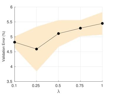


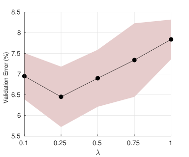

Although the fact that small validation sets limit the ability for model selection has been discussed in Chapelle et al. 2009, the work presented in Oliver et al. 2018 has used the Hoeffding inequality Hoeffding 1994 to directly analyze the relationship between the size of validation set and the variance in estimation of a model’s accuracy:
In this inequality, denotes the empirical estimate of the validation error, is its hypothetical true value, is the desired maximum deviation between the estimation and the true value, and represents the number of samples in the validation set. Based on this inequality, the number of samples in the validation set should be very large. For example, we will require about 20,000 samples in the validation set if we want to be 95% confident in estimation of validation error that differes less than 1% from the absolute true value. Note that in this analysis, validation error is computed as the average of independent binary indicator variables representing if a given sample in the validation set is classified correctly or not. This analysis may be unrealistic because of the assumption that the validation accuracy is the average of independent variables. To address this problem, Oliver et al. Oliver et al. 2018 measure this phenomenon empirically, and train the SSL methods using 1,000 labels in the training set from SVHN dataset and then evaluate them on the validation sets with different sizes. Note that these small synthetic validation sets are generated by different randomly sampled sets without overlapping from the full SVHN validation set. Following the same setting for evaluation of our SSL algorithm (ROT) in a real world scenario, in Fig. 3(a) and Fig. 4(a), we reported the mean and standard deviation of validation errors over five times randomly non-overlapping splitting the SVHN and CIFAR validation sets with varying sizes. The results in Fig. 3(a) and Fig. 4(a) indicate that as we increase the size of validation set, the ROT algorithm will be more confident and stable to select its hyperparameters than the case where we use small-size validation set. For a fair comparison between our method and the other SSL methods in Table. 1 of the paper, we have been consistent with other methods in the size of the training and validation sets as it is designed in standard SVHN and CIFAR-10 datasets. Specifically, for SVHN, we used 65,932 images for the training set and 7,325 for the validation set, and for CIFAR-10 dataset, we used 45,000 images for the training set and 5,000 images for the validation set. Fig. 3(b) and Fig. 4(b) indicate the error rate of the ROT algorithm on the SVHN and CIFAR validation sets for different values of in our transportation plan. Note that during the tuning of , we fixed in Eq. (5) to one and changed to different values including 0.1, 0.25, 0.5 , 0.75 and 1. Moreover, during the tuning of , we fixed in Eq. (3) to 0.25 and changed to different values including 0.1, 0.25, 0.5 , 0.75 and 1. Fig. 3(c) and Fig. 4(c) show the error rate of the ROT algorithm on the SVHN and CIFAR validation sets for different values of for training the parameters of the CNN.