Coefficientwise total positivity of some matrices defined by linear recurrences

A finite or infinite matrix with integer or real coefficients is called totally positive if all its minors are nonnegative, and strictly totally positive if all its minors are strictly positive.¹¹ 1 Warning: Many authors (e.g. [6, 5, 4]) use the terms ”totally nonnegative” and ”totally positive” for what we have termed ”totally positive” and ”strictly totally positive”, respectively. Such matrices have a wide variety of applications across pure and applied mathematics; background material on this topic can be found in [7, 6, 8, 4]. Many interesting lower-triangular matrices (hereafter simply referred to as triangles) that arise in combinatorics have been shown to be totally positive: well-known examples include the binomial coefficients $\binom{n}{k}$, the Stirling cycle numbers $\genfrac{[}{]}{0.0pt}{}{n}{k}$, and the Stirling subset numbers $\genfrac{}{}{0.0pt}{}{n}{k}$. But there are also many other combinatorially interesting triangles that appear to be totally positive but for which we have no proof. Foremost among these is what we call the "clean Eulerian triangle"

which was conjectured by Brenti [3] to be totally positive, already a quarter of a century ago.²² 2 Note that there exist several different conventions for the Eulerian triangle. For our purposes, the ”clean” version defined here is the most convenient, as it has 1’s both on the diagonal and in the zeroth column and is reversal-symmetric (i.e. $\genfrac{}{}{0.0pt}{}{n}{k}^{\!\rm clean}=\genfrac{}{}{0.0pt}{}{n}{n-k}^{\!\rm clean}$). It is easy to see that the other versions are totally positive if and only if the ”clean” one is. Here $\genfrac{}{}{0.0pt}{}{n}{k}^{\!\rm clean}$ is the number of permutations of $[n+1]$ with $k$ excedances (or $k$ descents), or the number of increasing binary trees on the vertex set $[n+1]$ with $k$ left children. These numbers satisfy the recurrence

for $n\geq 1$, with initial condition $\genfrac{}{}{0.0pt}{}{0}{k}^{\!\rm clean}=\delta_{k0}$.

A similar problem concerns the reversed Stirling subset triangle. Recall that the Stirling subset number $\genfrac{}{}{0.0pt}{}{n}{k}$ is the number of partitions of an $n$-element set into $k$ non-empty blocks [9, A048993/A008277]. We then write $\genfrac{}{}{0.0pt}{}{n}{k}^{\rm rev}=\genfrac{}{}{0.0pt}{}{n}{n-k}$. The reversed Stirling subset triangle is [9, A008278]

These numbers satisfy the recurrence

for $n\geq 1$, with initial condition $\genfrac{}{}{0.0pt}{}{0}{k}^{\!\rm rev}=\delta_{k0}$. Please note that the total positivity of a lower-triangular matrix does not in general imply the total positivity of its reversal. Nevertheless we conjecture:

In this extended abstract we present a more general triangle comprised of polynomial entries in six indeterminates that appears empirically to be coefficientwise totally positive and that yields, under suitable specialisations, both $\bm{A}$ and $\bm{S}^{\rm rev}$. We do not yet have any proof that this more general triangle is totally positive; indeed, we do not yet have any proof of Conjecture 1.1. But we are able to prove a special case that includes a generalisation of Conjecture 1.2.

Before stating our main conjecture, we extend the notion of total positivity to matrices whose elements are polynomials in one or more indeterminates ${\mathbf{x}}$. We equip the polynomial ring ${\mathbb{R}}[{\mathbf{x}}]$ with the coefficientwise partial order: that is, we say that $P$ is nonnegative (and write $P\succeq 0$) in case $P$ is a polynomial with nonnegative coefficients. We then say that a matrix with entries in ${\mathbb{R}}[{\mathbf{x}}]$ is coefficientwise totally positive if all of its minors are polynomials with nonnegative coefficients.

Comparing recurrences (2) and (4) invites us to consider the more general linear recurrence

for $n\geq 1$, with initial condition $T(0,k)=\delta_{k0}$. Here $a,c,d,e$ could be integers or real numbers, but we prefer to treat them as algebraic indeterminates. Thus, the elements of the matrix ${\bm{T}}=(T(n,k))_{n,k\geq 0}$ belong to the polynomial ring ${\mathbb{Z}}[a,c,d,e]$, and we conjecture:

This, however, is not the end of the story. Inspired partly by the work of Brenti [2] and partly by our own experiments, we were led to consider the more general recurrence

for $n\geq 1$, with initial conditions $T(0,k)=\delta_{k0}$ and $T(-1,k)=0$. Again, we treat $a,c,d,e,f,g$ as algebraic indeterminates, so that the matrix elements $T(n,k)$ belong to the polynomial ring ${\mathbb{Z}}[a,c,d,e,f,g]$. Note that this family is invariant under the reversal $k\to n-k$ by interchanging $(a,c)\leftrightarrow(d,e)$ and leaving $f$ and $g$ unchanged:

Our main conjecture is the following:

Unfortunately, for the time being, Conjectures 1.1, 1.3 and 1.4 remain unproven. (We have verified Conjecture 1.4 up to $13\times 13$; this computation took 109 days CPU time.) The rest of this extended abstract is devoted to proving the following special case of Conjecture 1.3, which is of some interest in its own right:

The triangle that appears in Theorem 1.5 is a generalisation of the reversed Stirling subset triangle, and reduces to it when $(a,c,e)=(1,0,1)$; this proves Conjecture 1.2. In what follows we write ${\bm{T}}(a,c,d,e,f,g)$ for the matrix defined by (6), and ${\bm{T}}(a,c,d,e)={\bm{T}}(a,c,d,e,0,0)$ for the matrix defined by (5).

It is possible to prove Theorem 1.5 in at least two different ways: one algebraic, the other combinatorial. In this extended abstract we take the combinatorial path, leaving the algebraic arguments to a longer paper (currently under construction). Section 2 establishes combinatorial interpretations of the entries of ${\bm{T}}(a,c,0,e)$ and ${\bm{T}}(0,c,d,e)$ as generating polynomials for set partitions with suitable weights. In Section 3 we present a planar network $D^{\prime}$ and show — by two different arguments — that the corresponding path matrix is equal to ${\bm{T}}(a,c,0,e)$; Theorem 1.5 then follows by the Lindström–Gessel–Viennot lemma.

From the fundamental recurrence $\genfrac{}{}{0.0pt}{}{n}{k}=\genfrac{}{}{0.0pt}{}{n-1}{k-1}\,+\,k\,\genfrac{}{}{0.0pt}{}{n-1}{k}$ for the Stirling subset numbers and its consequence (4) for the reversed Stirling subset numbers, we see that the Stirling and reversed Stirling numbers correspond to the matrix ${\bm{T}}(a,c,d,e)$ with $(a,c,d,e)=(0,1,1,0)$ and $(1,0,0,1)$, respectively. Moreover, if one considers instead $\genfrac{}{}{0.0pt}{}{n+1}{k+1}$ and $\genfrac{}{}{0.0pt}{}{n+1}{k}^{\rm rev}$, then these matrices correspond to ${\bm{T}}(a,c,d,e)$ with $(a,c,d,e)=(0,1,1,1)$ and $(1,1,0,1)$, respectively. We will now show how to generalise the combinatorial interpretations of $\genfrac{}{}{0.0pt}{}{n+1}{k+1}$ and $\genfrac{}{}{0.0pt}{}{n+1}{k}^{\rm rev}$ in terms of set partitions to ${\bm{T}}(0,c,d,e)$ and ${\bm{T}}(a,c,0,e)$.

We write $\Pi_{n}$ (resp. $\Pi_{n,k}$) for the set of all partitions of the set $[n]$ into nonempty blocks (resp. into exactly $k$ nonempty blocks). For $i\in[n]$ and $\pi\in\Pi_{n}$, we write $\mathop{\rm smallest}\nolimits(\pi,i)$ for the smallest element of the block of $\pi$ that contains $i$. We then have:

Please note that if one restricts a partition $\pi\in\Pi_{n+1}$ to $[m]$ for some $m<n+1$ — let us call the result $\pi_{m}\in\Pi_{m}$ — then $w_{\pi}(i)=w_{\pi_{m}}(i)$ for $2\leq i\leq m$, because $\mathop{\rm smallest}\nolimits(\pi,i)=\mathop{\rm smallest}\nolimits(\pi_{m},i)$. This fact will play a key role in justifying the recurrences.

Here is another recurrence satisfied by these matrices, which will be useful later:

We remark that these recurrences, supplemented by the initial condition $T(0,k)=\delta_{k0}$, completely determine the matrices.

One very useful tool in proving the total positivity of a matrix is the famous Lindström–Gessel–Viennot (LGV) lemma [1, Chapter 32]. Consider an acyclic digraph $\cal D$ equipped with edge weights $w_{e}$ and a distinguished set of sources $U:=\{u_{0},u_{1},\ldots\}$ and sinks $V:=\{v_{0},v_{1},\ldots\}$. The weight $w(\mathcal{P})$ of a path $\mathcal{P}$ is the product of its edge weights; and we define the path matrix $\bm{P}:=(P(u_{n}\to v_{k}))_{n,k\geq 0}$ by $P(u_{n}\to v_{k})\coloneqq\sum_{\mathcal{P}\colon u_{n}\to v_{k}}w(\mathcal{P})$. Now assume further that the digraph $\cal D$ is planar and that the sources and sinks lie on the boundary of $\cal D$ in the order “first $U$ in reverse order, then $V$ in order”; we refer to this setup as a planar network. Then the collection of sources and sinks is fully compatible in the sense that, for any subset of sources $u_{n_{1}},\dots,u_{n_{r}}$ (with $n_{1}<n_{2}<\cdots<n_{r}$) and sinks $v_{k_{1}},\dots,v_{k_{r}}$ (with $k_{1}<k_{2}<\cdots<k_{r}$), the only permutation $\sigma\in{\mathfrak{S}}_{r}$ mapping each source $u_{n_{i}}$ to the sink $v_{k_{\sigma(i)}}$ that gives rise to a nonempty family of nonintersecting paths in $\cal D$ is the identity permutation. The LGV lemma then implies that every minor of the path matrix $\bm{P}$ is given by a sum over families of nonintersecting paths between specified subsets of $U$ and $V$, where each family has weight $\prod w(\mathcal{P}_{i})$. If furthermore every edge weight $w_{e}$ is a positive real number, then $\bm{P}$ is totally positive; and if every edge weight is a polynomial in some indeterminates ${\mathbf{x}}$ with nonnegative real coefficients, then $\bm{P}$ is coefficientwise totally positive. This argument goes back to Brenti [2].

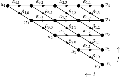
Figure 1(a) shows what we call the standard binomial-like planar network, which we denote $D$. We label the vertices of $D$ by pairs $(i,j)$ with $0\leq i\leq j$, where $i$ increases from right to left and $j$ increases from bottom to top. The horizontal directed edge from $(i,j)$ to $(i-1,j)$ [where $1\leq i\leq j$] is given a weight $\alpha_{i,j-i+1}$, while the diagonal directed edge from $(i,j)$ to $(i-1,j-1)$ [where $1\leq i\leq j$] is given a weight $\beta_{i,j-i}$. The source vertices are $u_{n}=(n,n)$ and the sink vertices are $v_{k}=(0,k)$.

It is easy to see that if the weights are purely $i$-dependent, then

so that the entries of the corresponding path matrix satisfy a purely $n$-dependent linear recurrence. Similarly, if the weights are purely $j$-dependent, then

so that the entries of the corresponding path matrix satisfy a purely $k$-dependent recurrence. In particular, by setting $\alpha_{i,j}=1$ and $\beta_{i,j}=j$, we recover a digraph yielding the Stirling subset triangle $P(u_{n}\to v_{k})=\genfrac{}{}{0.0pt}{}{n}{k}$; and more generally, by setting $\alpha_{i,j}=c$ and $\beta_{i,j}=jd+e$, we recover ${\bm{T}}(0,c,d,e)$ and prove its coefficientwise total positivity. This too goes back to Brenti [2].

We wish to thank Sergey Fomin for helpful correspondence. This research was supported in part by the U.K. Engineering and Physical Sciences Research Council grant EP/N025636/1, a fellowship from the China Scholarship Council, and a fellowship from the Deutsche Forschungsgemeinschaft.

References

- [1] M. Aigner and G.M. Ziegler, Proofs from THE BOOK, 6th ed. (Springer-Verlag, Berlin–Heidelberg, 2018).
- [2] F. Brenti, Combinatorics and total positivity, J. Combin. Theory A 71, 175–218 (1995).
- [3] F. Brenti, The applications of total positivity to combinatorics, and conversely. In: Total Positivity and its Applications, edited by M. Gasca and C.A. Micchelli (Kluwer, Dordrecht, 1996), pp. 451–473.
- [4] S.M. Fallat and C.R. Johnson, Totally Nonnegative Matrices (Princeton University Press, Princeton NJ, 2011).
- [5] S. Fomin and A. Zelevinsky, Total positivity: tests and parametrizations, Math. Intelligencer 22, no. 1, 23–33 (2000).
- [6] F.R. Gantmacher and M.G. Krein, Oscillation Matrices and Kernels and Small Vibrations of Mechanical Systems (AMS Chelsea Publishing, Providence RI, 2002). Based on the second Russian edition, 1950.
- [7] S. Karlin, Total Positivity (Stanford University Press, Stanford CA, 1968).
- [8] A. Pinkus, Totally Positive Matrices (Cambridge University Press, Cambridge, 2010).
- [9] The On-Line Encyclopedia of Integer Sequences, published electronically at http://oeis.org