An eXtended HDG method for Darcy-Stokes-Brinkman interface problems Thanks: This work was supported in part by National Natural Science Foundation of China (11771312).

Yihui Han Thanks: South China Research Center for Applied Mathematics and Interdisciplinary Studies, South China Normal University, Guangzhou, 510630, China, Email: yhhan@m.scnu.edu.cn Xiao-Ping Wang Thanks: Department of Mathematics, The Hong Kong University of Science and Technology, Clear Water Bay, Kowloon, Hong Kong, China, Email: mawang@ust.hk Xiaoping Xie Thanks: Corresponding author. School of Mathematics, Sichuan University, Chengdu 610064, China, Email: xpxie@scu.edu.cn

Abstract

This paper proposes an interface/boundary-unfitted eXtended hybridizable discontinuous Galerkin (X-HDG) method for Darcy-Stokes-Brinkman interface problems in two and three dimensions. The method uses piecewise linear polynomials for the velocity approximation and piecewise constants for both the velocity gradient and pressure approximations in the interior of elements inside the subdomains separated by the interface, uses piecewise constants for the numerical traces of velocity on the inter-element boundaries inside the subdomains, and uses piecewise constants or linear polynomials for the numerical traces of velocity on the interface. Optimal error estimates are derived for the interface-unfitted X-HDG scheme. Numerical experiments are provided to verify the theoretical results and the robustness of the proposed method.

$\bf{Key}$ $\bf{Words}$ : eXtended HDG method, Darcy-Stokes-Brinkman interface problem, interface/boundary-unfitted mesh, error estimate.

1 Introduction

Let $\Omega\subset\mathbb{R}^{d}(d=2,3)$ be a bounded domain divided into two subdomains, $\Omega_{i}(i=1,2)$ , by a piecewise smooth interface $\Gamma$ (cf. Figure 1). We consider the following Darcy-Stokes-Brinkman interface problem: find the velocity $\bm{u}$ and the pressure $p$ such that

\displaystyle\left\{\begin{array}[]{rl}-\nabla\cdot(\nu\nabla\bm{u})+\nabla p+\alpha\bm{u}=\bm{f}&\text{in}\quad\Omega_{1}\cup\Omega_{2},\\ \nabla\cdot\bm{u}=0&\text{in}\quad\Omega_{1}\cup\Omega_{2},\\ \bm{u}=\bm{g}_{D}&\text{on}\quad\partial\Omega,\\ \llbracket\bm{u}\rrbracket=\bm{0},\ \llbracket(\nu\nabla\bm{u}-p\bm{I})\bm{n}\rrbracket=\bm{g}_{N}^{\Gamma}&\text{on}\quad\Gamma.\end{array}\right.

Here the viscosity coefficient $\nu$ and the zeroth-order term coefficient $\alpha$ are piecewise constants with

\displaystyle\nu|_{\Omega_{i}}=\nu_{i}>0,\hskip 10.00002pt\alpha|_{\Omega_{i}}=\alpha_{i}\geq 0,\hskip 10.00002pti=1,2.

(1.5)

The jump of a function $w$ across the interface $\Gamma$ is defined by $\llbracket w\rrbracket:=(w|_{\Omega_{1}})|_{\Gamma}-(w|_{\Omega_{2}})|_{\Gamma}$ , $\bm{I}$ the $d\times d$ identity matrix, and $\bm{n}$ denotes the unit normal vector along $\Gamma$ , pointing to $\Omega_{2}$ . $\bm{f}$ denotes the body force, $\bm{g}_{N}^{\Gamma}$ the interface traction, and $\bm{g}_{D}$ the source term satisfying

\displaystyle\int_{\partial\Omega}\bm{g}_{D}\cdot\bm{n}=0,

(1.6)

where $\bm{n}$ is the outward unit normal vector along $\partial\Omega$ . The Darcy-Stokes-Brinkman model (1) is usually used to describe porous media flow coupled with viscous fluid flow in a single form of equation (cf. [43, 49, 35, 23, 21]).

Refer to caption — Figure 1: The geometry of domain with circle interface or fold line interface

For an elliptic interface problem, the low regularity of the solution due to the coefficient discontinuity may result in reduced accuracy of finite element discretization [4, 50]. One strategy for this situation is to use interface(or body)-fitted meshes (cf. Figure 2) so as to dominate the approximation error caused by the non-smoothness of solution [7, 9, 14, 32, 44, 11]. However, the generation of interface-fitted meshes is usually expensive, especially when the interface is of complicated geometry or moving with time or iteration.

Another strategy avoiding the loss of numerical accuracy is to use certain modification of the finite element approximation around the interface. The resultant finite element methods do not need interface-fitted meshes (cf. Figure 2). One representative of such interface-unfitted methods is the eXtended/Generalized Finite Element Method (XFEM or GFEM), where additional basis functions characterizing the singularity of the solution around the interface are enriched into the corresponding approximation space. We refer to [45] for an overview work and [5, 8, 6, 10, 28, 48, 51] for some developments of XFEM/GFEM. In particular, we refer to [12, 15, 30, 29, 34, 47] for several XFEMs using additional cut basis functions for Stokes or Darcy interface problems. It should be pointed out that the immersed finite element method (IFEM) is another type of interface-unfitted method, where special finite element basis functions are constructed to satisfy the interface jump conditions (cf. [1, 2, 39, 40, 41, 52, 31] and the references therein).

The hybridizable discontinuous Galerkin (HDG) framework [16] provides a unifying strategy for hybridization of finite element methods for second order elliptic problems. By the local elimination of the unknowns defined in the interior of elements, the HDG method leads to a system where the unknowns are only the globally coupled degrees of freedom describing the introduced Lagrange multiplier. We refer to [42, 17, 18, 38, 36, 37, 20, 3, 22, 33, 19, 25, 24, 46] for some developments and applications of the HDG method. We also mention that arbitrary order interface-unfitted eXtended HDG methods with optimal convergence were analyzed in [26, 27] for elliptic and elasticity interface problems, respectively.

In this paper we aim to propose a low order eXtended HDG (X-HDG) method for the Darcy-Stokes-Brinkman interface problem (1). The main features of the method are as follows:

•

The method is a low order scheme, which uses piecewise linear polynomials for the velocity approximation and piecewise constants for both the velocity gradient and pressure approximations in the interior of elements inside the subdomains separated by the interface, and uses piecewise constants for the numerical traces of velocity on the inter-element boundaries inside the subdomains.
•

To deal with the interface conditions, the interface is approximated by a fold line/plane, on which the numerical traces of velocity adopt piecewise constants or piecewise linear polynomials.
•

The method is parametric-friendly in the sense that optimal error estimates are obtained without requiring “sufficiently large” stabilization parameters in the scheme.
•

The method uses interface-unfitted polygonal/polyhedral meshes, and applies to curved domains with boundary-unfitted meshes.

The rest of the paper is organized as follows. Section 2 introduces the X-HDG scheme for the interface problem with a polygonal/polyhedral domain. Section 3 is devoted to the error estimation. Section 4 applies the X-HDG method to a curved domain problem. Numerical examples are provided in Section 5 to verify the theoretical results. Finally, Section 6 gives some concluding remarks.

2 X-HDG scheme for interface problem

2.1 Notation and XFE spaces

For any bounded domain $D\subset\mathbb{R}^{s}$ $(s=d,d-1)$ and nonnegative integer $m$ , let $H^{m}(D)$ and $H_{0}^{m}(D)$ be the usual $m$ -th order Sobolev spaces on $D$ , with norm $\lVert\cdot\rVert_{m,D}$ and semi-norm $\lvert\cdot\rvert_{m,D}$ . In particular, $L^{2}(D):=H^{0}(D)$ is the space of square integrable functions, with inner product $(\cdot,\cdot)_{D}$ . When $D\subset R^{d-1}$ , we use $\langle\cdot,\cdot\rangle_{D}$ to replace $(\cdot,\cdot)_{D}$ . For $m=1,2$ , we set

	$\displaystyle H^{m}(\Omega_{1}\cup\Omega_{2}):=\{v\in L^{2}(\Omega),v\|_{\Omega_{1}}\in H^{m}(\Omega_{1}),\ \text{and}\ v\|_{\Omega_{2}}\in H^{m}(\Omega_{2})\},$
	$\displaystyle\lVert\cdot\rVert_{m}:=\lVert\cdot\rVert_{m,\Omega_{1}\cup\Omega_{2}}=\sum\limits_{i=1}^{2}\lVert\cdot\rVert_{m,\Omega_{i}},\hskip 10.00002pt\lvert\cdot\rvert_{m}:=\lvert\cdot\rvert_{m,\Omega_{1}\cup\Omega_{2}}=\sum\limits_{i=1}^{2}\lvert\cdot\rvert_{m,\Omega_{i}}.$

For any integer $k\geqslant 0$ , $P_{k}(D)$ denotes the set of all polynomials on D with degree at most $k$ .

Assume that $\Omega$ is a polygonal/polyhedral domain. Let $\mathcal{T}_{h}=\cup\{K\}$ , consisting of arbitrary open polygons/polyhedrons, be a shape-regular partition of the domain $\Omega$ in the sense that the following two assumptions hold (cf. [13]):

(M1). There exists a positive constant $\theta_{*}$ such that the following holds: for each element $K\in\mathcal{T}_{h}$ , there exists a point $M_{K}\in K$ such that $K$ is star-shaped with respect to every point in the circle (or sphere) of center $M_{K}$ and radius $\theta_{*}h_{K}$ .

(M2). There exists a positive constant $l_{*}$ such that for every element $K\in\mathcal{T}_{h}$ , the distance between any two vertexes is no less than $l_{*}h_{K}$ .

We define the set of all elements intersected by the interface $\Gamma$ as

\displaystyle\mathcal{T}_{h}^{\Gamma}:=\{K\in\mathcal{T}_{h}:K\cap\Gamma\neq\emptyset\}.

For any $K\in\mathcal{T}_{h}^{\Gamma}$ , called an interface element, let $\Gamma_{K}:=K\cap\Gamma$ be the part of $\Gamma$ in $K$ , and $\Gamma_{K,h}$ be the straight line/plane segment connecting the intersection between $\Gamma_{K}$ and $\partial K$ (Figure 4).

To ensure that $\Gamma$ is reasonably resolved by $\mathcal{T}_{h}$ , we make the following standard assumptions on $\mathcal{T}_{h}$ and $\Gamma$ ( cf. Figure 3 for two cases violating the assumptions):

(A1). For $K\in\mathcal{T}_{h}^{\Gamma}$ and any edge/face $F\subset\partial K$ which intersects $\Gamma$ , $F_{\Gamma}:=\Gamma\cap F$ is simply connected with either $F_{\Gamma}=F$ or $meas(F_{\Gamma})=0$ .

(A2). For $K\in\mathcal{T}_{h}^{\Gamma}$ , $\Gamma_{K}$ is sufficiently smooth such that for any two different points $\bm{x},\bm{y}\in\Gamma_{K}$ , the unit normal vectors $\bm{n}(\bm{x})$ and $\bm{n}(\bm{y})$ , pointing to $\Omega_{2}$ , at $\bm{x}$ and $\bm{y}$ satisfy

\displaystyle\lvert\bm{n}(\bm{x})-\bm{n}(\bm{y})\rvert\leq\gamma h_{K},

(2.1)

with $\gamma\geq 0$ (cf.[14, 50]). Note that $\gamma=0$ when $\Gamma_{K}=\Gamma_{K,h}$ , i.e. $\Gamma_{K}$ is a straight line/plane segment.

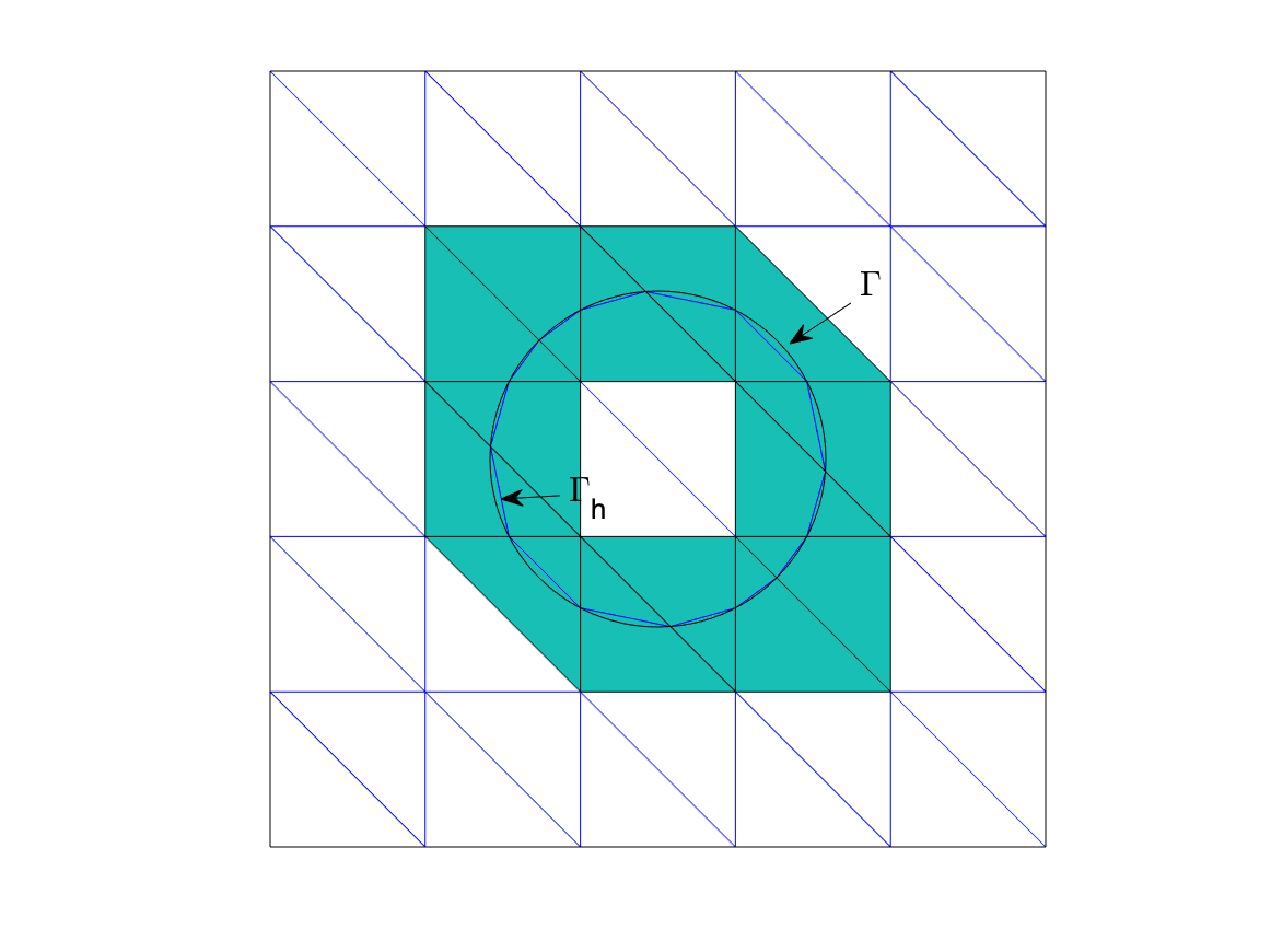
Let $\mathcal{\varepsilon}_{h}$ be the set of all edges(faces) of all elements in $\mathcal{T}_{h}$ . Denote by $\mathcal{\varepsilon}_{h}^{\Gamma}$ the partition of the fold line/plane approximation of $\Gamma$ with respect to $\mathcal{T}_{h}$ , i.e.

\mathcal{\varepsilon}_{h}^{\Gamma}:=\{F:\ F=\Gamma_{K,h},\text{ or }F=\Gamma\cap\partial K\text{ if $\Gamma\cap\partial K$ is an edge/face of $K$},\ K\in\mathcal{T}_{h}\}.

We set $\mathcal{\varepsilon}_{h}^{*}:=\mathcal{\varepsilon}_{h}\setminus\mathcal{\varepsilon}_{h}^{\Gamma}$ . For any $K\in\mathcal{T}_{h}$ and $F\in\mathcal{\varepsilon}_{h}^{*}\cup\mathcal{\varepsilon}_{h}^{\Gamma},$ let $h_{K}$ and $h_{F}$ be respectively the diameters of $K$ and $F$ , and let $\bm{n}_{K}$ be the unit outward normal vector along $\partial K$ . Denote by $h:=\max\limits_{K\in\mathcal{T}_{h}}h_{K}$ the mesh size of $\mathcal{T}_{h}$ , and by $\nabla_{h}$ and $\nabla_{h}\cdot$ the piecewise-defined gradient and divergence operators with respect to $\mathcal{T}_{h}$ , respectively.

Since the rest of the paper deals with the discrete problem, in what follows and without ambiguity, let $\Omega_{1}$ and $\Omega_{2}$ denote the two sides of $\Gamma_{h}$ rather than of $\Gamma$ , and set $K_{i}=K\cap\Omega_{i}$ for $i=1,2$ .

Throughout the paper, we use $a\lesssim b$ $(a\apprge b)$ to denote $a\leq Cb$ $(a\geq Cb)$ , where $C$ is a generic positive constant independent of mesh parameters $h,h_{K},h_{e}$ , the coefficients $\nu_{i},\alpha_{i}$ $(i=1,2)$ and the location of the interface relative to the mesh.

2.2 X-HDG scheme

The X-HDG method is based on the following first-order formulations of Darcy-Stokes-Brinkman interface problem (1):


$\displaystyle\bm{L}=\nu\nabla\bm{u}$	$\displaystyle\hskip 10.00002pt\text{in}\hskip 10.00002pt\Omega_{1}\cup\Omega_{2},$	(2.2a)
$\displaystyle-\nabla\cdot\bm{L}+\nabla p+\alpha\bm{u}=\bm{f}$	$\displaystyle\hskip 10.00002pt\text{in}\hskip 10.00002pt\Omega_{1}\cup\Omega_{2},$	(2.2b)
$\displaystyle\nabla\cdot\bm{u}=0$	$\displaystyle\hskip 10.00002pt\text{in}\hskip 10.00002pt\Omega_{1}\cup\Omega_{2},$	(2.2c)
$\displaystyle\bm{u}=\bm{g}_{D}$	$\displaystyle\hskip 10.00002pt\text{on}\hskip 10.00002pt\partial\Omega,$	(2.2d)
$\displaystyle\llbracket\bm{u}\rrbracket=\bm{0},\ \llbracket(\bm{L}-p\bm{I})\bm{n}\rrbracket=\bm{g}_{N}^{\Gamma}$	$\displaystyle\hskip 10.00002pt\text{on}\hskip 10.00002pt\Gamma.$	(2.2e)

Let $\chi_{i}$ be the characteristic function on $\Omega_{i}$ for $i=1,2$ . For any integer $r\geq 0$ , $F\in\mathcal{\varepsilon}_{h}^{*}\cup\mathcal{\varepsilon}_{h}^{\Gamma}$ and $K\in\mathcal{T}_{h}$ , let $Q_{r}^{b}:L^{2}(D)\rightarrow P_{r}(D)$ and $Q_{r}:L^{2}(\tilde{D})\rightarrow P_{r}(\tilde{D})$ be the standard $L^{2}$ orthogonal projection operators for $D=F\cap\bar{\Omega}_{i}$ and $\tilde{D}=K\cap\Omega_{i}$ , respectively. Vector or tensor analogues of $Q_{r}^{b}$ and $Q_{r}$ are denoted by $\bm{Q}_{r}^{b}$ and $\bm{Q}_{r}$ , respectively. Set

\oplus\chi_{i}P_{r}(K):=\chi_{1}P_{r}(K)+\chi_{2}P_{r}(K),\hskip 10.00002ptr=0,1.

We introduce the following X-HDG finite element spaces:

	$\displaystyle\bm{W}_{h}=$	$\displaystyle\{\bm{w}\in L^{2}(\Omega)^{d\times d}:\ \forall K\in\mathcal{T}_{h},\bm{w}\|_{K}\in P_{0}(K)^{d\times d}\ \text{if}\ K\cap\Gamma=\varnothing;\bm{w}\|_{K}\in(\oplus\chi_{i}P_{0}(K))^{d\times d}\ \text{if}\ K\cap\Gamma\neq\varnothing\},$
	$\displaystyle\bm{V}_{h}=$	$\displaystyle\{\bm{v}\in L^{2}(\Omega)^{d}:\ \forall K\in\mathcal{T}_{h},\bm{v}\|_{K}\in P_{1}(K)^{d}\ \text{if}\ K\cap\Gamma=\varnothing;\bm{v}\|_{K}\in(\oplus\chi_{i}P_{1}(K))^{d}\ \text{if}\ K\cap\Gamma\neq\varnothing\},$
	$\displaystyle Q_{h}=$	$\displaystyle\{q\in L_{0}^{2}(\Omega):\ \forall K\in\mathcal{T}_{h},q\|_{K}\in P_{0}(K)\ \text{if}\ K\cap\Gamma=\varnothing;q\|_{K}\in\oplus\chi_{i}P_{0}(K)\ \text{if}\ K\cap\Gamma\neq\varnothing\},$
	$\displaystyle\bm{M}_{h}=$	$\displaystyle\{\bm{\mu}\in L^{2}(\varepsilon_{h}^{})^{d}:\forall F\in\varepsilon_{h}^{},\bm{\mu}\|_{F}\in P_{0}(F)^{d}\ \text{if}\ F\cap\Gamma=\varnothing;\bm{\mu}\|_{F}\in(\oplus\chi_{i}P_{0}(F))^{d}\ \text{if}\ F\cap\Gamma\neq\varnothing\},$
	$\displaystyle\bm{\tilde{M}_{h}}=$	$\displaystyle\{\tilde{\bm{\mu}}\in L^{2}(\mathcal{\varepsilon}_{h}^{\Gamma})^{d}:\tilde{\bm{\mu}}\|_{F}\in P_{m}(F)^{d},\forall F\in\mathcal{\varepsilon}_{h}^{\Gamma}\}\text{ with }m=0\text{ or }1,$
	$\displaystyle\bm{M}_{h}(\bm{g}_{D})=$	$\displaystyle\{\bm{\mu}\in\bm{M}_{h}:\bm{\mu}\|_{F}=\bm{Q}_{0}^{b}\bm{g}_{D},\forall F\in\varepsilon_{h}\text{ with }F\subset\partial\Omega\}.$

To describe the X-HDG scheme, we also define

\displaystyle(\cdot,\cdot)_{\mathcal{T}_{h}}:=\sum\limits_{K\in\mathcal{T}_{h}}(\cdot,\cdot)_{K},\hskip 10.00002pt\langle\cdot,\cdot\rangle_{\partial\mathcal{T}_{h}\setminus\mathcal{\varepsilon}_{h}^{\Gamma}}:=\sum\limits_{K\in\mathcal{T}_{h}}\langle\cdot,\cdot\rangle_{\partial K\backslash\mathcal{\varepsilon}_{h}^{\Gamma}},

and, for scalars $q$ , vector $\bm{u},\bm{v}$ and tensor $\bm{w}$ with $q_{i}=q|_{\bar{\Omega}_{i}\cap F},\bm{u}_{i}=\bm{u}|_{\bar{\Omega}_{i}\cap F},\bm{v}_{i}=\bm{v}|_{\bar{\Omega}_{i}\cap F}$ and $\bm{w}_{i}=\bm{w}|_{\bar{\Omega}_{i}\cap F}$ ,

	$\displaystyle\langle q,\bm{v}\cdot\bm{n}\rangle_{*,\mathcal{\varepsilon}_{h}^{\Gamma}}:$	$\displaystyle=\sum\limits_{F\in\mathcal{\varepsilon}_{h}^{\Gamma}}\langle q_{1},\bm{v}_{1}\cdot\bm{n}_{1}\rangle_{\bar{\Omega}_{1}\cap F}+\langle q_{2},\bm{v}_{2}\cdot\bm{n}_{2}\rangle_{\bar{\Omega}_{2}\cap F},$
	$\displaystyle\langle\bm{u},\bm{v}\rangle_{*,\mathcal{\varepsilon}_{h}^{\Gamma}}:$	$\displaystyle=\sum\limits_{F\in\mathcal{\varepsilon}_{h}^{\Gamma}}\langle\bm{u}_{1},\bm{v}_{1}\rangle_{\bar{\Omega}_{1}\cap F}+\langle\bm{u}_{2},\bm{v}_{2}\rangle_{\bar{\Omega}_{2}\cap F},$
	$\displaystyle\langle\bm{w}\bm{n},\bm{v}\rangle_{*,\mathcal{\varepsilon}_{h}^{\Gamma}}:$	$\displaystyle=\sum\limits_{F\in\mathcal{\varepsilon}_{h}^{\Gamma}}\langle\bm{w}_{1}\bm{n}_{1},\bm{v}_{1}\rangle_{\bar{\Omega}_{1}\cap F}+\langle\bm{w}_{2}\bm{n}_{2},\bm{v}_{2}\rangle_{\bar{\Omega}_{2}\cap F},$

where $\bm{n}_{i}$ denotes the unit normal vector along $\Gamma_{h}$ pointing from $\Omega_{i}$ to $\Omega_{j}$ with $i,j=1,2$ and $i\neq j$ .

The eXtended HDG method seeks $(\bm{L}_{h},\bm{u}_{h},p_{h},\bm{\hat{u}}_{h},\bm{\tilde{u}}_{h})\in\bm{W}_{h}\times\bm{V_{h}}\times Q_{h}\times\bm{M}_{h}(\bm{g}_{D})\times\bm{\tilde{M}_{h}}$ satisfying


$\displaystyle(\nu^{-1}\bm{L}_{h},\bm{w})_{\mathcal{T}_{h}}-\langle\hat{\bm{u}}_{h},\bm{w}\bm{n}\rangle_{\partial\mathcal{T}_{h}\setminus\mathcal{\varepsilon}_{h}^{\Gamma}}-\langle\tilde{\bm{u}}_{h},\bm{w}\bm{n}\rangle_{*,\mathcal{\varepsilon}_{h}^{\Gamma}}=$	$\displaystyle 0,$	(2.3a)
$\displaystyle(\alpha\bm{u}_{h},\bm{v})_{\mathcal{T}_{h}}+\langle\tau(\bm{Q}_{0}^{b}\bm{u}_{h}-\bm{\hat{u}}_{h}),\bm{v}\rangle_{\partial\mathcal{T}_{h}\setminus\mathcal{\varepsilon}_{h}^{\Gamma}}+\langle\tau(\bm{Q}_{m}^{b}\bm{u}_{h}-\bm{\tilde{u}}_{h}),\bm{v}\rangle_{*,\mathcal{\varepsilon}_{h}^{\Gamma}}=$	$\displaystyle(\bm{f},\bm{v}),$	(2.3b)
$\displaystyle\langle\bm{\hat{u}}_{h}\cdot\bm{n},q\rangle_{\partial\mathcal{T}_{h}\setminus\mathcal{\varepsilon}_{h}^{\Gamma}}+\langle\bm{\tilde{u}}_{h}\cdot\bm{n},q\rangle_{*,\mathcal{\varepsilon}_{h}^{\Gamma}}=$	$\displaystyle 0,$	(2.3c)
$\displaystyle\langle\bm{L}_{h}\bm{n},\bm{\mu}\rangle_{\partial\mathcal{T}_{h}\setminus\mathcal{\varepsilon}_{h}^{\Gamma}}-\langle p_{h}\bm{n},\bm{\mu}\rangle_{\partial\mathcal{T}_{h}\setminus\mathcal{\varepsilon}_{h}^{\Gamma}}-\langle\tau(\bm{Q}_{0}^{b}\bm{u}_{h}-\bm{\hat{u}}_{h}),\bm{\mu}\rangle_{\partial\mathcal{T}_{h}\setminus\mathcal{\varepsilon}_{h}^{\Gamma}}=$	$\displaystyle 0,$	(2.3d)
$\displaystyle\langle\bm{L}_{h}\bm{n},\bm{\tilde{\mu}}\rangle_{,\mathcal{\varepsilon}_{h}^{\Gamma}}-\langle p_{h}\bm{n},\bm{\tilde{\mu}}\rangle_{,\mathcal{\varepsilon}_{h}^{\Gamma}}-\langle\tau(\bm{Q}_{m}^{b}\bm{u}_{h}-\bm{\tilde{u}}_{h}),\bm{\tilde{\mu}}\rangle_{*,\mathcal{\varepsilon}_{h}^{\Gamma}}=$	$\displaystyle\langle\bm{g}_{N}^{\Gamma_{h}},\bm{\tilde{\mu}}\rangle_{*,\mathcal{\varepsilon}_{h}^{\Gamma}},$	(2.3e)

for all $(\bm{w},\bm{v},q,\bm{\mu},\bm{\tilde{\mu}})\in\bm{W}_{h}\times\bm{V_{h}}\times Q_{h}\times\bm{M}_{h}(0)\times\bm{\tilde{M}_{h}}$ . Here the stabilization function $\tau$ is defined as following: for any $K\in\mathcal{T}_{h}$ and $i=1,2$ ,

\displaystyle\tau|_{F\cap\bar{\Omega}_{i}}

\displaystyle=\nu_{i}h_{K}^{-1},\hskip 10.00002pt{\rm for}\ F\subset\partial K\setminus{\mathcal{\varepsilon}_{h}^{\Gamma}}\ {\rm or}\ F\in\mathcal{\varepsilon}_{h}^{\Gamma}.

(2.4)

When $F\in\mathcal{\varepsilon}_{h}^{\Gamma}$ is a line segment/straight plane, we take $\bm{g}_{N}^{\Gamma_{h}}|_{F}:=\bm{g}_{N}^{\Gamma}$ , and when $F=\Gamma_{K,h}\neq\Gamma_{K}$ for some $K\in\mathcal{T}_{h}^{\Gamma}$ , we set $\bm{g}_{N}^{\Gamma_{h}}|_{F}$ to be some linear interpolation of $\bm{g}_{N}^{\Gamma}$ using data of $\bm{g}_{N}^{\Gamma}$ at two (2D case) /three (3D case) intersection points of $\Gamma_{K}$ and $\Gamma_{K,h}$ .

Remark 2.1.

From the first-order system (2.2), there should be some terms like $(\bm{u}_{h},\nabla_{h}\cdot\bm{w})_{\mathcal{T}_{h}}$ , $-(\nabla_{h}\cdot\bm{L}_{h},\bm{v})_{\mathcal{T}_{h}}$ , $(\nabla_{h}p_{h},\bm{v})_{\mathcal{T}_{h}}$ , and $-(\bm{u}_{h},\nabla q)_{\mathcal{T}_{h}}$ in the scheme (2.3). In fact, they are all vanish since $\bm{W}_{h}$ and $Q_{h}$ are piecewise constant tensor/scalar spaces.

Remark 2.2.

We note that in the implementation, we can locally eliminate the $\bm{L}_{h},\bm{u}_{h}$ defined in the interior of elements, and the reduced system only involves the unknowns of $p_{h}$ , $\hat{\bm{u}}_{h}$ and $\tilde{\bm{u}}_{h}$ .

Theorem 2.1.

The X-HDG scheme (2.3) (with $m=0$ or $1$ ) admits a unique solution.

Proof.

Since the (2.3) is a linear square system, it suffices to show that if all of the given data vanish, i.e. $\bm{f}=\bm{g}_{D}=\bm{g}_{N}^{\Gamma_{h}}=0$ , then we get the zero solution. By taking the $(\bm{w},\bm{v},q,\bm{\mu},\bm{\tilde{\mu}})=(\bm{L}_{h},\bm{u}_{h},p_{h},\bm{\hat{u}_{h}},\bm{\tilde{u}_{h}})$ in (2.3) and adding these equations together, we have

\displaystyle(\nu^{-1}\bm{L}_{h},\bm{L}_{h})_{\mathcal{T}_{h}}+(\alpha\bm{u}_{h},\bm{u}_{h})_{\mathcal{T}_{h}}+\langle\tau(\bm{Q}_{0}^{b}\bm{u}_{h}-\bm{\hat{u}}_{h}),(\bm{u}_{h}-\bm{\hat{u}}_{h})\rangle_{\partial\mathcal{T}_{h}\setminus\mathcal{\varepsilon}_{h}^{\Gamma}}+\langle\tau(\bm{Q}_{m}^{b}\bm{u}_{h}-\bm{\tilde{u}}_{h}),(\bm{u}_{h}-\bm{\tilde{u}}_{h})\rangle_{*,\mathcal{\varepsilon}_{h}^{\Gamma}}=0,

which indicates $\bm{L}_{h}=\bm{0}$ ,

	$\displaystyle\bm{Q}_{0}^{b}\bm{u}_{h}-\bm{\hat{u}}_{h}$	$\displaystyle=\bm{0},\hskip 10.00002pt\text{ on}\ \partial K\setminus\mathcal{\varepsilon}_{h}^{\Gamma},\forall K\in\mathcal{T}_{h},$		(2.5)
	$\displaystyle\{\bm{Q}_{m}^{b}\bm{u}_{h}-\bm{\tilde{u}}_{h}\}$	$\displaystyle=\bm{0},\hskip 10.00002pt\text{ on}\ \mathcal{\varepsilon}_{h}^{\Gamma}.$		(2.6)

where $\{\cdot\}$ is defined by $\{w\}=\frac{1}{2}(w_{1}+w_{2})$ with $w_{i}=w|_{\bar{\Omega}_{i}\cap\Gamma}$ for $i=1,2$ . These relations, together with the equation (2.3a), the definition of projection and integration by parts, yield

\displaystyle 0=(\nu^{-1}\bm{L}_{h},\bm{w})_{\mathcal{T}_{h}}+(\nabla_{h}\bm{u}_{h},\bm{w})_{\mathcal{T}_{h}}-\langle\bm{Q}_{0}^{b}\bm{u}_{h}-\bm{\hat{u}}_{h},\bm{w}\bm{n}\rangle_{\partial\mathcal{T}_{h}\setminus\mathcal{\varepsilon}_{h}^{\Gamma}}-\langle\bm{Q}_{m}^{b}\bm{u}_{h}-\bm{\tilde{u}}_{h},\bm{w}\bm{n}\rangle_{*,\mathcal{\varepsilon}_{h}^{\Gamma}}=(\nabla_{h}\bm{u}_{h},\bm{w})_{\mathcal{T}_{h}}.

Taking the $\bm{w}_{h}=\nabla_{h}\bm{u}_{h}$ in this relation gives $\nabla_{h}\bm{u}_{h}=\bm{0}$ . Then $\bm{u}_{h}$ is piecewise constant, which, together with (2.5), (2.6) and the fact that $\bm{\hat{u}}_{h}=\bm{0}$ on $\partial\Omega$ , implies

\displaystyle\bm{u}_{h}=\bm{\hat{u}}_{h}=\bm{\tilde{u}}_{h}=\bm{0}.

The thing left is to show $p_{h}=0$ . In view of (2.3d) and (2.3e), we have

\displaystyle\llbracket p_{h}\rrbracket=0,

\displaystyle\ \text{ on}\ \partial K\text{ and }\mathcal{\varepsilon}_{h}^{\Gamma},\forall K\in\mathcal{T}_{h}.

Thus, $p_{h}$ is a constant in $\Omega$ , and the fact $p_{h}\in L_{0}^{2}(\Omega)$ means $p_{h}=0$ . This completes the proof. ∎

3 A priori error estimation: a case of fold line/plane interface

This section is devoted to an error analysis of the X-HDG scheme (2.3) with a fold line/plane interface $\Gamma$ . We note that in this case $\Gamma_{K}=\Gamma_{K,h}$ is a line segment/quadrilateral for any $K\in\mathcal{T}_{h}^{\Gamma}$ , and $\bm{g}_{N}^{\Gamma_{h}}=\bm{g}_{N}^{\Gamma}$ in the equation (2.3e).

3.1 Optimal error estimation for velocity gradient and pressure

Firstly we introduce the following standard estimates for the $L^{2}$ orthogonal projection operators $Q_{r}$ and $Q_{r}^{b}$ (cf. [13, 26]).

Lemma 3.1.

Let $s$ be an integer with $1\leq s\leq r+1$ . For any $K\in\mathcal{T}_{h}$ and $v\in H^{s}\left((K\cap\Omega_{1})\cup(K\cap\Omega_{2})\right)$ , we have

	$\displaystyle\lVert v-Q_{r}v\rVert_{0,K}+h\lVert v-Q_{r}v\rVert_{1,K}$	$\displaystyle\lesssim h_{K}^{s}\lVert v\rVert_{s,K},$
	$\displaystyle\lVert v-Q_{r}v\rVert_{0,\partial K}+\lVert v-Q_{r}v\rVert_{0,\Gamma_{K}}$	$\displaystyle\lesssim h_{K}^{s-1/2}\lVert v\rVert_{s,K},$
	$\displaystyle\lVert v-Q_{r}^{b}v\rVert_{0,\partial K}+\lVert v-Q_{r}^{b}v\rVert_{0,\Gamma_{K}}$	$\displaystyle\lesssim h_{K}^{s-1/2}\lVert v\rVert_{s,K},$

where the notations $\lVert\cdot\rVert_{s,K}$ and $\lVert\cdot\rVert_{0,\partial K}$ are understood respectively as $\lVert\cdot\rVert_{s,K}=\sum\limits_{i=1}^{2}\lVert\cdot\rVert_{s,K\cap\Omega_{i}}$ and $\lVert\cdot\rVert_{s,\partial K}=\sum\limits_{i=1}^{2}\lVert\cdot\rVert_{s,\partial K\cap\bar{\Omega}_{i}}$ when $K\in\mathcal{T}_{h}^{\Gamma}$ .

For simplicity of presentation, denote

\displaystyle\bm{e}_{h}^{L}:

\displaystyle=\bm{L}_{h}-\bm{Q}_{0}\bm{L},\hskip 10.00002pt\bm{e}_{h}^{u}:=\bm{u}_{h}-\bm{Q}_{1}\bm{u},\hskip 10.00002pte_{h}^{p}:=p_{h}-Q_{0}p,\hskip 10.00002pt\bm{e}_{h}^{\hat{u}}:=\bm{\hat{u}}_{h}-\bm{Q}_{0}^{b}\bm{u},\hskip 10.00002pt\bm{e}_{h}^{\tilde{u}}:=\bm{\tilde{u}}_{h}-\bm{Q}_{m}^{b}\bm{u},

(3.1)

where, for $i=1,2$ and $m=0,1$ ,

		$\displaystyle(\bm{Q}_{0}\bm{L})\|_{K\cap\Omega_{i}}:=\bm{Q}_{0}(\bm{L}\|_{K\cap\Omega_{i}}),\hskip 10.00002pt(\bm{Q}_{1}\bm{u})\|_{K\cap\Omega_{i}}:=\bm{Q}_{1}(\bm{u}\|_{K\cap\Omega_{i}}),\ \hskip 10.00002pt(Q_{0}p)\|_{K\cap\Omega_{i}}:=Q_{0}(p\|_{K\cap\Omega_{i}}),\hskip 10.00002pt\forall K\in\mathcal{T}_{h},$
		$\displaystyle(\bm{Q}_{0}^{b}\bm{u})\|_{F\cap\Omega_{i}}:=\bm{Q}_{0}^{b}(\bm{u}\|_{F\cap\Omega_{i}}),\hskip 10.00002pt\forall F\in\varepsilon_{h}^{*},$
		$\displaystyle(\bm{Q}_{m}^{b}\bm{u})\|_{F}:=\bm{Q}_{m}^{b}(\bm{u}\|_{F}),\hskip 10.00002pt\forall F\in\mathcal{\varepsilon}_{h}^{\Gamma}.$

Then we have the following lemma for error equations.

Lemma 3.2.

For all $(\bm{w},\bm{v},q,\bm{\mu},\bm{\tilde{\mu}})\in\bm{W}_{h}\times\bm{V}_{h}\times Q_{h}\times\bm{M}_{h}(0)\times\bm{\tilde{M}}_{h}$ , it holds


$\displaystyle(\nu^{-1}\bm{e}_{h}^{L},\bm{w})_{\mathcal{T}_{h}}-\langle\bm{e}_{h}^{\hat{u}},\bm{w}\bm{n}\rangle_{\partial\mathcal{T}_{h}\setminus\mathcal{\varepsilon}_{h}^{\Gamma}}-\langle\bm{e}_{h}^{\tilde{u}},\bm{w}\bm{n}\rangle_{*,\mathcal{\varepsilon}_{h}^{\Gamma}}$	$\displaystyle=0,$	(3.2a)
$\displaystyle(\alpha\bm{e}_{h}^{u},\bm{v})_{\mathcal{T}_{h}}+\langle\tau(Q_{0}^{b}\bm{e}_{h}^{u}-\bm{e}_{h}^{\hat{u}}),\bm{v}\rangle_{\partial\mathcal{T}_{h}\setminus\mathcal{\varepsilon}_{h}^{\Gamma}}+\langle\tau(Q_{m}^{b}\bm{e}_{h}^{u}-\bm{e}_{h}^{\tilde{u}}),\bm{v}\rangle_{*,\mathcal{\varepsilon}_{h}^{\Gamma}}$	$\displaystyle=\sum_{i=1}^{2}L_{i}(\bm{v}),$	(3.2b)
$\displaystyle\langle\bm{e}_{h}^{\hat{u}}\cdot\bm{n},q\rangle_{\partial\mathcal{T}_{h}\setminus\mathcal{\varepsilon}_{h}^{\Gamma}}+\langle\bm{e}_{h}^{\tilde{u}}\cdot\bm{n},q\rangle_{*,\mathcal{\varepsilon}_{h}^{\Gamma}}$	$\displaystyle=0,$	(3.2c)
$\displaystyle\langle\bm{e}_{h}^{L}\bm{n},\bm{\mu}\rangle_{\partial\mathcal{T}_{h}\setminus\mathcal{\varepsilon}_{h}^{\Gamma}}-\langle e_{h}^{p}\bm{n},\bm{\mu}\rangle_{\partial\mathcal{T}_{h}\setminus\mathcal{\varepsilon}_{h}^{\Gamma}}-\langle\tau(Q_{0}^{b}\bm{e}_{h}^{u}-\bm{e}_{h}^{\hat{u}}),\bm{\mu}\rangle_{\partial\mathcal{T}_{h}\setminus\mathcal{\varepsilon}_{h}^{\Gamma}}$	$\displaystyle=-L_{1}(\bm{\mu}),$	(3.2d)
$\displaystyle\langle\bm{e}_{h}^{L}\bm{n},\bm{\tilde{\mu}}\rangle_{,\mathcal{\varepsilon}_{h}^{\Gamma}}-\langle e_{h}^{p}\bm{n},\bm{\tilde{\mu}}\rangle_{,\mathcal{\varepsilon}_{h}^{\Gamma}}-\langle\tau(Q_{m}^{b}\bm{e}_{h}^{u}-\bm{e}_{h}^{\tilde{u}}),\bm{\tilde{\mu}}\rangle_{*,\mathcal{\varepsilon}_{h}^{\Gamma}}$	$\displaystyle=-L_{2}(\bm{\tilde{\mu}}),$	(3.2e)

where for any $\psi\in H^{1}(\Omega_{1}\cup\Omega_{2})\cup\bm{W}_{h}\cup\bm{V}_{h}\cup\bm{M}_{h}\cup\bm{\tilde{M}}_{h}$ ,

	$\displaystyle L_{1}(\psi)$	$\displaystyle=\langle(\bm{Q}_{0}\bm{L}-\bm{L})\bm{n},\psi\rangle_{\partial\mathcal{T}_{h}\setminus\mathcal{\varepsilon}_{h}^{\Gamma}}+\langle\tau(\bm{Q}_{0}^{b}(\bm{u}-\bm{Q}_{1}\bm{u})),\psi\rangle_{\partial\mathcal{T}_{h}\setminus\mathcal{\varepsilon}_{h}^{\Gamma}}+\langle(Q_{0}p-p)\bm{n},\psi\rangle_{\partial\mathcal{T}_{h}\setminus\mathcal{\varepsilon}_{h}^{\Gamma}},$
	$\displaystyle L_{2}(\psi)$	$\displaystyle=\langle(\bm{Q}_{0}\bm{L}-\bm{L})\bm{n},\psi\rangle_{,\mathcal{\varepsilon}_{h}^{\Gamma}}+\langle\tau(\bm{Q}_{m}^{b}(\bm{u}-\bm{Q}_{1}\bm{u})),\psi\rangle_{,\mathcal{\varepsilon}_{h}^{\Gamma}}+\langle(Q_{0}p-p)\bm{n},\psi\rangle_{*,\mathcal{\varepsilon}_{h}^{\Gamma}}.$

Proof.

Let $(\bm{L},\bm{u},p)$ be the solution of (2.2). From the definitions of the projection operators we obtain

	$\displaystyle(\nu^{-1}\bm{Q}_{0}\bm{L},\bm{w})_{\mathcal{T}_{h}}-\langle\bm{Q}_{0}^{b}\bm{u},\bm{w}\bm{n}\rangle_{\partial\mathcal{T}_{h}\setminus\mathcal{\varepsilon}_{h}^{\Gamma}}-\langle\bm{Q}_{m}^{b}\bm{u},\bm{w}\bm{n}\rangle_{*,\mathcal{\varepsilon}_{h}^{\Gamma}}$	$\displaystyle=0,$
	$\displaystyle\langle(\bm{Q}_{0}\bm{L}-\bm{L})\bm{n},\bm{v}\rangle_{\partial\mathcal{T}_{h}\setminus\mathcal{\varepsilon}_{h}^{\Gamma}}+\langle(\bm{Q}_{0}\bm{L}-\bm{L})\bm{n},\bm{v}\rangle_{*,\mathcal{\varepsilon}_{h}^{\Gamma}}+(\alpha\bm{Q}_{1}\bm{u},\bm{v}\rangle_{\mathcal{T}_{h}}$
	$\displaystyle-\langle(Q_{0}p-p)\bm{n},\bm{v}\rangle_{\partial\mathcal{T}_{h}\setminus\mathcal{\varepsilon}_{h}^{\Gamma}}-\langle(Q_{0}p-p)\bm{n},\bm{v}\rangle_{*,\mathcal{\varepsilon}_{h}^{\Gamma}}$	$\displaystyle=(\bm{f},\bm{v}),$
	$\displaystyle\langle\bm{Q}_{0}^{b}\bm{u}\cdot\bm{n},q\rangle_{\partial\mathcal{T}_{h}\setminus\mathcal{\varepsilon}_{h}^{\Gamma}}+\langle\bm{Q}_{0}^{b}\bm{u}\cdot\bm{n},q\rangle_{*,\mathcal{\varepsilon}_{h}^{\Gamma}}$	$\displaystyle=0,$

for any $(\bm{w},\bm{v},q)\in\bm{W}_{h}\times\bm{V}_{h}\times Q_{h}$ . Then, subtracting (2.3a), (2.3b) and (2.3c) respectively from the above three equations yields (3.2a), (3.2b) and (3.2c). Finally, (3.2d), (3.2e) follows from (2.3d), (2.3e) and the relations

\displaystyle\langle(\bm{L}-p\bm{I})\bm{n},\bm{\bm{\mu}}\rangle_{\partial\mathcal{T}_{h}\setminus\mathcal{\varepsilon}_{h}^{\Gamma}}=\bm{0},\hskip 10.00002pt\langle(\bm{L}-p\bm{I})\bm{n},\bm{\tilde{\mu}}\rangle_{\mathcal{\varepsilon}_{h}^{\Gamma}}=\langle\bm{g}_{N}^{\Gamma_{h}},\bm{\tilde{\mu}}\rangle_{\mathcal{\varepsilon}_{h}^{\Gamma}}

for $\bm{\mu}\in\bm{M}_{h}(0),\ \bm{\tilde{\mu}}\in\bm{\tilde{M}}_{h}$ . ∎

Define a seminorm $\interleave\cdot\interleave:\bm{w},\bm{v},\bm{\mu},\bm{\tilde{\mu}}\in{L^{2}}(\Omega)^{d\times d}\times{L^{2}}(\Omega)^{d}\times{L}^{2}(\varepsilon_{h}^{*})^{d}\times{L^{2}}(\ \varepsilon_{h}^{\Gamma})^{d}$ by

\displaystyle\interleave(\bm{w},\bm{v},\bm{\mu},\tilde{\mu})\interleave^{2}:=\lVert\nu^{-\frac{1}{2}}\bm{w}\rVert_{0,\mathcal{T}_{h}}^{2}+\lVert\alpha^{\frac{1}{2}}\bm{v}\rVert_{0,\mathcal{T}_{h}}^{2}+\lVert\tau^{1/2}(\bm{Q}_{0}^{b}\bm{v}-\bm{\mu})\rVert_{\partial\mathcal{T}_{h}\setminus\mathcal{\varepsilon}_{h}^{\Gamma}}^{2}+\lVert\tau^{1/2}(\bm{Q}_{m}^{b}\bm{v}-\bm{\tilde{\mu}})\rVert_{*,\mathcal{\varepsilon}_{h}^{\Gamma}}^{2},

(3.3)

where

\lVert\cdot\rVert_{0,\mathcal{T}_{h}}^{2}:=\sum_{K\in\mathcal{T}_{h}}\lVert\cdot\rVert_{0,K}^{2},\ \ \lVert\cdot\rVert_{\partial\mathcal{T}_{h}\setminus\varepsilon_{h}^{\Gamma}}^{2}:=\sum\limits_{K\in\mathcal{T}_{h}}\langle\cdot,\cdot\rangle_{\partial K\backslash\varepsilon_{h}^{\Gamma}},\ \ \lVert\cdot\rVert_{\varepsilon_{h}^{\Gamma}}^{2}:=\langle\cdot,\cdot\rangle_{*,\varepsilon_{h}^{\Gamma}}.

Lemma 3.3.

Let $(\bm{L},\bm{u},p)\in{H^{1}}(\Omega_{1}\cup\Omega_{2})^{d\times d}\times{H^{2}}(\Omega_{1}\cup\Omega_{2})^{d}\times H^{1}(\Omega_{1}\cup\Omega_{2})$ and $(\bm{L}_{h},\bm{u}_{h},p_{h},\bm{\hat{u}}_{h},\bm{\tilde{u}}_{h})\in\bm{W}_{h}\times V_{h}\times Q_{h}\times M_{h}(g)\times\tilde{M}_{h}$ be the solutions of the problem (2.2) and the X-HDG scheme (2.3), respectively. Then it holds

\displaystyle\lVert\nu^{\frac{1}{2}}\nabla_{h}\bm{e}_{h}^{u}\rVert_{0,\mathcal{T}_{h}}\lesssim\interleave(\bm{e}_{h}^{L},\bm{e}_{h}^{u},\bm{e}_{h}^{\hat{u}},\bm{e}_{h}^{\tilde{u}})\interleave\lesssim h(\lVert\nu^{\frac{1}{2}}\bm{u}\rVert_{2,\Omega_{1}\cup\Omega_{2}}+\lVert\nu^{-\frac{1}{2}}p\rVert_{1,\Omega_{1}\cup\Omega_{2}}).

(3.4)

Proof.

We first show

\displaystyle\lVert\nu^{\frac{1}{2}}\nabla_{h}\bm{e}_{h}^{u}\rVert_{0,\mathcal{T}_{h}}\lesssim\interleave(\bm{e}_{h}^{L},\bm{e}_{h}^{u},\bm{e}_{h}^{\hat{u}},\bm{e}_{h}^{\tilde{u}})\interleave.

(3.5)

In fact, taking $\bm{w}=\nu\nabla\bm{e}_{h}^{u}$ in (3.2a) and applying integration by parts yield

\displaystyle(\bm{e}_{h}^{L},\nabla\bm{e}_{h}^{u})_{\mathcal{T}_{h}}-(\nu\nabla\bm{e}_{h}^{u},\nabla\bm{e}_{h}^{u})_{\mathcal{T}_{h}}-\langle\nu(\bm{e}_{h}^{u}-\bm{e}_{h}^{\hat{u}}),\nabla\bm{e}_{h}^{u}\bm{n}\rangle_{\partial\mathcal{T}_{h}\setminus\mathcal{\varepsilon}_{h}^{\Gamma}}-\langle\nu(\bm{e}_{h}^{u}-\bm{e}_{h}^{\tilde{u}}),\nabla\bm{e}_{h}^{u}\bm{n}\rangle_{*,\mathcal{\varepsilon}_{h}^{\Gamma}}

\displaystyle=0,

which, together with the property of projection, implies

\displaystyle\lVert\nu^{\frac{1}{2}}\nabla\bm{e}_{h}^{u}\rVert_{0,\mathcal{T}_{h}}^{2}=(\bm{e}_{h}^{L},\nabla\bm{e}_{h}^{u})_{{\mathcal{T}_{h}}}-\langle\nu(\bm{Q}_{0}^{b}\bm{e}_{h}^{u}-\bm{e}_{h}^{\hat{u}}),\nabla\bm{e}_{h}^{u}\bm{n}\rangle_{\partial\mathcal{T}_{h}\setminus\mathcal{\varepsilon}_{h}^{\Gamma}}-\langle\nu(\bm{Q}_{m}^{b}\bm{e}_{h}^{u}-\bm{e}_{h}^{\tilde{u}}),\nabla\bm{e}_{h}^{u}\bm{n}\rangle_{*,\mathcal{\varepsilon}_{h}^{\Gamma}}

for $m=0,1$ . In view of the Cauchy-Schwarz inequality, the trace inequality and the definition of $\interleave\cdot\interleave$ , we then have

\displaystyle\lVert\nu^{\frac{1}{2}}\nabla\bm{e}_{h}^{u}\rVert_{0,\mathcal{T}_{h}}\leq\lVert\nu^{-\frac{1}{2}}\bm{e}_{h}^{L}\rVert_{0,\mathcal{T}_{h}}+\lVert\tau^{1/2}(\bm{Q}_{0}^{b}\bm{e}_{h}^{u}-\bm{e}_{h}^{\hat{u}})\rVert_{\partial\mathcal{T}_{h}\setminus\mathcal{\varepsilon}_{h}^{\Gamma}}+\lVert\tau^{1/2}(\bm{Q}_{m}^{b}\bm{e}_{h}^{u}-\bm{e}_{h}^{\tilde{u}})\rVert_{\mathcal{\varepsilon}_{h}^{\Gamma}}\leq\interleave(\bm{e}_{h}^{L},\bm{e}_{h}^{u},\bm{e}_{h}^{\hat{u}},\bm{e}_{h}^{\tilde{\mu}})\interleave,

where we recall that $\tau$ is given by (2.4).

The thing left is to estimate the term $\interleave(\bm{e}_{h}^{L},\bm{e}_{h}^{u},\bm{e}_{h}^{\hat{u}},\bm{e}_{h}^{\tilde{\mu}})\interleave$ . Taking $(\bm{w},\bm{v},q,\bm{\mu},\bm{\tilde{\mu}})=(\bm{e}_{h}^{L},\bm{e}_{h}^{u},e_{h}^{p},\bm{e}_{h}^{\hat{u}},\bm{e}_{h}^{\tilde{\mu}})$ in (3.2) and adding up the five equations, we obtain

\interleave(\bm{e}_{h}^{L},\bm{e}_{h}^{u},\bm{e}_{h}^{\hat{u}},\bm{e}_{h}^{\tilde{\mu}})\interleave^{2}=\sum_{i=1}^{2}E_{i},

where

	$\displaystyle E_{1}$	$\displaystyle=\langle(\bm{Q}_{0}\bm{L}-\bm{L})\bm{n},\bm{e}_{h}^{u}-\bm{e}_{h}^{\hat{u}}\rangle_{\partial\mathcal{T}_{h}\setminus\mathcal{\varepsilon}_{h}^{\Gamma}}+\langle(\bm{Q}_{0}\bm{L}-\bm{L})\bm{n},\bm{e}_{h}^{u}-\bm{e}_{h}^{\tilde{u}}\rangle_{*,\mathcal{\varepsilon}_{h}^{\Gamma}}$
		$\displaystyle\hskip 20.00003pt+\langle(Q_{0}p-p)\bm{n},\bm{e}_{h}^{u}-\bm{e}_{h}^{\hat{u}}\rangle_{\partial\mathcal{T}_{h}\setminus\mathcal{\varepsilon}_{h}^{\Gamma}}+\langle(Q_{0}p-p)\bm{n},\bm{e}_{h}^{u}-\bm{e}_{h}^{\tilde{u}}\rangle_{*,\mathcal{\varepsilon}_{h}^{\Gamma}},$
	$\displaystyle E_{2}$	$\displaystyle=\langle\tau\bm{Q}_{0}^{b}(\bm{u}-\bm{Q}_{1}\bm{u}),\bm{e}_{h}^{u}-\bm{e}_{h}^{\hat{u}}\rangle_{\partial\mathcal{T}_{h}\setminus\mathcal{\varepsilon}_{h}^{\Gamma}}+\langle\tau\bm{Q}_{m}^{b}(\bm{u}-\bm{Q}_{1}\bm{u}),\bm{e}_{h}^{u}-\bm{e}_{h}^{\tilde{u}}\rangle_{*,\mathcal{\varepsilon}_{h}^{\Gamma}}.$

We just need to estimate $E_{i}$ ( $i=1,2$ ) term by term. From Lemma 3.1, the Cauchy-Schwarz inequality and (3.5) it follows

	$\displaystyle E_{1}\lesssim$	$\displaystyle h\big(\lVert\nu^{-\frac{1}{2}}\bm{L}\rVert_{1,\Omega_{1}\cup\Omega_{2}}+\lVert\nu^{-\frac{1}{2}}p\rVert_{1,\Omega_{1}\cup\Omega_{2}}\big)\big(\lVert\tau^{\frac{1}{2}}(\bm{e}_{h}^{u}-\bm{e}_{h}^{\hat{u}})\rVert_{0,\partial\mathcal{T}_{h}\setminus\mathcal{\varepsilon}_{h}^{\Gamma}}+\lVert\tau^{\frac{1}{2}}(\bm{e}_{h}^{u}-\bm{e}_{h}^{\tilde{u}})\rVert_{\mathcal{\varepsilon}_{h}^{\Gamma}}\big)$
	$\displaystyle\lesssim$	$\displaystyle h\big(\lVert\nu^{-\frac{1}{2}}\bm{L}\rVert_{1,\Omega_{1}\cup\Omega_{2}}+\lVert\nu^{-\frac{1}{2}}p\rVert_{1,\Omega_{1}\cup\Omega_{2}}\big)\big(\lVert\tau^{\frac{1}{2}}(\bm{Q}_{0}^{b}\bm{e}_{h}^{u}-\bm{e}_{h}^{\hat{u}})\rVert_{0,\partial\mathcal{T}_{h}\setminus\mathcal{\varepsilon}_{h}^{\Gamma}}+\lVert\tau^{\frac{1}{2}}(\bm{Q}_{m}^{b}\bm{e}_{h}^{u}-\bm{e}_{h}^{\tilde{u}})\rVert_{\mathcal{\varepsilon}_{h}^{\Gamma}}$
		$\displaystyle\hskip 10.00002pt+\lVert\tau^{\frac{1}{2}}(\bm{e}_{h}^{u}-\bm{Q}_{0}^{b}\bm{e}_{h}^{u})\rVert_{0,\partial\mathcal{T}_{h}\setminus\mathcal{\varepsilon}_{h}^{\Gamma}}+\lVert\tau^{\frac{1}{2}}(\bm{e}_{h}^{u}-\bm{Q}_{m}^{b}\bm{e}_{h}^{u})\rVert_{\mathcal{\varepsilon}_{h}^{\Gamma}}\big)$
	$\displaystyle\lesssim$	$\displaystyle h\big(\lVert\nu^{-\frac{1}{2}}\bm{L}\rVert_{1,\Omega_{1}\cup\Omega_{2}}+\lVert\nu^{-\frac{1}{2}}p\rVert_{1,\Omega_{1}\cup\Omega_{2}}\big)\big(\interleave(\bm{e}_{h}^{L},\bm{e}_{h}^{u},\bm{e}_{h}^{\hat{u}},\bm{e}_{h}^{\tilde{u}})\interleave+\lVert\nu^{\frac{1}{2}}\nabla_{h}\bm{e}_{h}^{u}\rVert_{0,\mathcal{T}_{h}}\big)$
	$\displaystyle\lesssim$	$\displaystyle h\big(\lVert\nu^{\frac{1}{2}}\bm{u}\rVert_{2,\Omega_{1}\cup\Omega_{2}}+\lVert\nu^{-\frac{1}{2}}p\rVert_{1,\Omega_{1}\cup\Omega_{2}}\big)\interleave(\bm{e}_{h}^{L},\bm{e}_{h}^{u},\bm{e}_{h}^{\hat{u}},\bm{e}_{h}^{\tilde{u}})\interleave.$

Similarly, we have

	$\displaystyle E_{2}\leq$	$\displaystyle\big(\lVert\tau(\bm{u}-\bm{Q}_{1}\bm{u})\rVert_{0,\partial\mathcal{T}_{h}\setminus\mathcal{\varepsilon}_{h}^{\Gamma}}+\lVert\tau(\bm{u}-\bm{Q}_{1}\bm{u})\rVert_{0,\mathcal{\varepsilon}_{h}^{\Gamma}}\big)\big(\lVert\tau^{\frac{1}{2}}(\bm{e}_{h}^{u}-\bm{e}_{h}^{\hat{u}})\rVert_{0,\partial\mathcal{T}_{h}\setminus\mathcal{\varepsilon}_{h}^{\Gamma}}+\lVert\tau^{\frac{1}{2}}(\bm{e}_{h}^{u}-\bm{e}_{h}^{\tilde{u}})\rVert_{\mathcal{\varepsilon}_{h}^{\Gamma}}\big)$
	$\displaystyle\lesssim$	$\displaystyle h\lVert\nu^{\frac{1}{2}}\bm{u}\rVert_{2,\Omega_{1}\cup\Omega_{2}}\interleave(\bm{e}_{h}^{L},\bm{e}_{h}^{u},\bm{e}_{h}^{\hat{u}},\bm{e}_{h}^{\tilde{u}})\interleave.$

As a result, the desired conclusion follows. ∎

Lemma 3.4.

Under the same conditions as in Lemma 3.3, it holds

\displaystyle\lVert e_{h}^{p}\rVert_{0,\mathcal{T}_{h}}\lesssim h(\nu_{max}^{\frac{1}{2}}+\alpha_{max}^{\frac{1}{2}})\left(\lVert\nu^{\frac{1}{2}}\bm{u}\rVert_{2,\Omega_{1}\cup\Omega_{2}}+\lVert\nu^{-\frac{1}{2}}p\rVert_{1,\Omega_{1}\cup\Omega_{2}}\right).

(3.6)

Here $\nu_{max}=\max\limits_{i=1,2}{\nu_{i}}$ and $\alpha_{max}=\max\limits_{i=1,2}{\alpha_{i}}$ .

Proof.

Since $e_{h}^{p}\in L_{0}^{2}(\Omega)$ , there exists $\bm{v^{*}}\in H_{0}^{1}(\Omega)$ such that

\displaystyle\lVert e_{h}^{p}\rVert_{0,\mathcal{T}_{h}}\lesssim\frac{(\nabla\cdot\bm{v^{*}},e_{h}^{p})}{\lVert\bm{v^{*}}\rVert_{1,\Omega_{1}\cup\Omega_{2}}}.

(3.7)

In view of integration by parts, the properties of projections, and (3.2b), (3.2d) and (3.2e) with $(\bm{v},\bm{\mu},\bm{\tilde{\mu}})=(\bm{\bm{Q}_{1}v^{*}},\bm{Q}_{0}^{b}\bm{v^{*}},\bm{Q}_{m}^{b}\bm{v^{*}})$ , we have

\displaystyle(\nabla\cdot\bm{v^{*}},e_{h}^{p})_{\mathcal{T}_{h}}=

\displaystyle\langle\bm{Q}_{0}^{b}\bm{v^{*}},e_{h}^{p}\bm{n}\rangle_{\partial\mathcal{T}_{h}\setminus\mathcal{\varepsilon}_{h}^{\Gamma}}+\langle\bm{Q}_{m}^{b}\bm{v^{*}},e_{h}^{p}\bm{n}\rangle_{*,\mathcal{\varepsilon}_{h}^{\Gamma}}=T_{1}+T_{2}+T_{3},

where

	$\displaystyle T_{1}=$	$\displaystyle\langle\bm{e}_{h}^{L}\bm{n},\bm{Q}_{0}^{b}\bm{v^{}}\rangle_{\partial\mathcal{T}_{h}\setminus\mathcal{\varepsilon}_{h}^{\Gamma}}+\langle\bm{e}_{h}^{L}\bm{n},\bm{Q}_{m}^{b}\bm{v^{}}\rangle_{,\mathcal{\varepsilon}_{h}^{\Gamma}}+(\alpha\bm{e}_{h}^{u},\bm{Q}_{1}\bm{v^{}})_{\mathcal{T}_{h}},$
	$\displaystyle T_{2}=$	$\displaystyle\langle\tau(\bm{Q}_{0}^{b}\bm{e}_{h}^{u}-\bm{e}_{h}^{\hat{u}}),\bm{Q}_{1}\bm{v^{}}-\bm{Q}_{0}^{b}\bm{v^{}}\rangle_{\partial\mathcal{T}_{h}\setminus\mathcal{\varepsilon}_{h}^{\Gamma}}+\langle\tau(\bm{Q}_{m}^{b}\bm{e}_{h}^{u}-\bm{e}_{h}^{\tilde{u}}),\bm{Q}_{1}\bm{v^{}}-\bm{Q}_{m}^{b}\bm{v^{}}\rangle_{*,\mathcal{\varepsilon}_{h}^{\Gamma}},$
	$\displaystyle T_{3}=$	$\displaystyle-L_{1}(\bm{Q}_{1}\bm{v^{}}-\bm{Q}_{0}^{b}\bm{v^{}})-L_{2}(\bm{Q}_{1}\bm{v^{}}-\bm{Q}_{m}^{b}\bm{v^{}}).$

From integration by parts, the Cauchy-Schwarz inequality and the properties of projections it follows

	$\displaystyle T_{1}=$	$\displaystyle\ \ (\bm{e}_{h}^{L},\nabla_{h}\bm{Q}_{1}\bm{v^{}})_{\mathcal{T}_{h}}+\langle\bm{e}_{h}^{L}\bm{n},\bm{Q}_{1}\bm{v^{}}-\bm{Q}_{0}^{b}\bm{v^{}}\rangle_{\partial\mathcal{T}_{h}\setminus\mathcal{\varepsilon}_{h}^{\Gamma}}+\langle\bm{e}_{h}^{L}\bm{n},\bm{Q}_{1}\bm{v^{}}-\bm{Q}_{m}^{b}\bm{v^{}}\rangle_{,\mathcal{\varepsilon}_{h}^{\Gamma}}+(\alpha\bm{e}_{h}^{u},\bm{Q}_{1}\bm{v^{*}})_{\mathcal{T}_{h}}$
	$\displaystyle\lesssim$	$\displaystyle\ \ \left(\nu_{max}^{\frac{1}{2}}\lVert\nu^{-\frac{1}{2}}\bm{e}_{h}^{L}\rVert_{0,\mathcal{T}_{h}}+\alpha_{max}^{\frac{1}{2}}\lVert\alpha^{\frac{1}{2}}\bm{e}_{h}^{u}\rVert_{0,\mathcal{T}_{h}}\right)\lVert\bm{v^{*}}\rVert_{1,\Omega}$
	$\displaystyle\lesssim$	$\displaystyle\ \ (\nu_{max}^{\frac{1}{2}}+\alpha_{max}^{\frac{1}{2}})\interleave(\bm{e}_{h}^{L},\bm{e}_{h}^{u},\bm{e}_{h}^{\hat{u}},\bm{e}_{h}^{\tilde{u}})\interleave\lVert\bm{v^{*}}\rVert_{1,\Omega},$
	$\displaystyle T_{2}\lesssim$	$\displaystyle\ \ \nu_{max}^{\frac{1}{2}}\interleave(\bm{e}_{h}^{L},\bm{e}_{h}^{u},\bm{e}_{h}^{\hat{u}},\bm{e}_{h}^{\tilde{u}})\interleave\lVert\bm{v^{*}}\rVert_{1,\Omega},$
	$\displaystyle T_{3}\lesssim$	$\displaystyle\ \ \nu_{max}^{\frac{1}{2}}h\left(\lVert\nu^{-\frac{1}{2}}\bm{L}\rVert_{1,\Omega_{1}\cup\Omega_{2}}+\lVert\nu^{\frac{1}{2}}\bm{u}\rVert_{2,\Omega_{1}\cup\Omega_{2}}+\lVert\nu^{-\frac{1}{2}}p\rVert_{1,\Omega_{1}\cup\Omega_{2}}\right)\lVert\bm{v^{*}}\rVert_{1,\Omega}.$

So by (3.7) and the relation (2.2a) we have

\displaystyle\lVert e_{h}^{p}\rVert_{0,\mathcal{T}_{h}}\lesssim(\nu_{max}^{\frac{1}{2}}+\alpha_{max}^{\frac{1}{2}})\left(\interleave(\bm{e}_{h}^{L},\bm{e}_{h}^{u},\bm{e}_{h}^{\hat{u}},\bm{e}_{h}^{\tilde{u}})\interleave+h(\lVert\nu^{\frac{1}{2}}\bm{u}\rVert_{2,\Omega_{1}\cup\Omega_{2}}+\lVert\nu^{-\frac{1}{2}}p\rVert_{1,\Omega_{1}\cup\Omega_{2}}\right),

which, together with Lemma 3.3, yields the desired result (3.6). ∎

Based on Lemmas 3.1, 3.3, 3.4, and the triangle inequality, we can easily obtain the following main result.

Theorem 3.1.

$\displaystyle\lVert\nu^{-\frac{1}{2}}(\bm{L}-\bm{L}_{h})\rVert_{0,\mathcal{T}_{h}}$	$\displaystyle+\lVert\nu^{\frac{1}{2}}(\nabla\bm{u}-\nabla_{h}\bm{u}_{h})\rVert_{0,\mathcal{T}_{h}}+(\nu_{max}^{\frac{1}{2}}+\alpha_{max}^{\frac{1}{2}})^{-1}\lVert p-p_{h}\rVert_{0,\mathcal{T}_{h}}$
	$\displaystyle\lesssim h\left(\lVert\nu^{\frac{1}{2}}\bm{u}\rVert_{2,\Omega_{1}\cup\Omega_{2}}+\lVert\nu^{-\frac{1}{2}}p\rVert_{1,\Omega_{1}\cup\Omega_{2}}\right),$	(3.8)
$\displaystyle\lVert\alpha^{\frac{1}{2}}(\bm{u}-\bm{u}_{h})\rVert_{0,\mathcal{T}_{h}}$	$\displaystyle\lesssim h\left(\lVert\nu^{\frac{1}{2}}\bm{u}\rVert_{2,\Omega_{1}\cup\Omega_{2}}+\lVert\alpha^{\frac{1}{2}}\bm{u}\rVert_{1,\Omega_{1}\cup\Omega_{2}}+\lVert\nu^{-\frac{1}{2}}p\rVert_{1,\Omega_{1}\cup\Omega_{2}}\right).$	(3.9)

3.2 $L^{2}$ error estimation for velocity

In this subsection, we shall derive an $L^{2}$ error estimate for the velocity approximation by the Aubin-Nitsche’s technique of duality argument. To this end, we introduce the auxiliary problem


$\displaystyle\bm{\Phi}=\nu\nabla\bm{\phi}$	$\displaystyle\hskip 10.00002pt\text{in}\hskip 10.00002pt\Omega_{1}\cup\Omega_{2},$	(3.10a)
$\displaystyle-\nabla\cdot\bm{\Phi}+\nabla\psi+\alpha\bm{\phi}=\bm{e}_{h}^{u}$	$\displaystyle\hskip 10.00002pt\text{in}\hskip 10.00002pt\Omega_{1}\cup\Omega_{2},$	(3.10b)
$\displaystyle\nabla\cdot\bm{\phi}=0$	$\displaystyle\hskip 10.00002pt\text{in}\hskip 10.00002pt\Omega_{1}\cup\Omega_{2},$	(3.10c)
$\displaystyle\bm{\phi}=\bm{0}$	$\displaystyle\hskip 10.00002pt\text{on}\hskip 10.00002pt\partial\Omega,$	(3.10d)
$\displaystyle\llbracket\bm{\phi}\rrbracket=\bm{0},\ \llbracket(\bm{\Phi}-\psi\bm{I})\bm{n}\rrbracket=\bm{0}$	$\displaystyle\hskip 10.00002pt\text{on}\hskip 10.00002pt\Gamma,$	(3.10e)

and assume the following regularity estimate:

\displaystyle\lVert\bm{\Phi}\rVert_{1,\Omega_{1}\cup\Omega_{2}}+\lVert\nu\bm{\phi}\rVert_{2,\Omega_{1}\cup\Omega_{2}}+\lVert\alpha\bm{\phi}\rVert_{2,\Omega_{1}\cup\Omega_{2}}+\lVert\psi\rVert_{1,\Omega_{1}\cup\Omega_{2}}\lesssim\lVert\bm{e}_{h}^{u}\rVert_{0,\mathcal{T}_{h}}.

(3.11)

Here we recall that $\bm{e}_{h}^{u}=\bm{u}_{h}-\bm{Q}_{1}\bm{u}$ .

Theorem 3.2.

\displaystyle\lVert\bm{u}-\bm{u}_{h}\rVert_{0,\mathcal{T}_{h}}\lesssim h^{2}\nu_{min}^{-\frac{1}{2}}\left(\lVert\nu^{\frac{1}{2}}\bm{u}\rVert_{2,\Omega_{1}\cup\Omega_{2}}+\lVert\nu^{-\frac{1}{2}}p\rVert_{1,\Omega_{1}\cup\Omega_{2}}\right)

(3.12)

for (i) $m=1$ or (ii) $m=0$ and $\bm{g}_{N}^{\Gamma}$ is a constant on any $F\in\mathcal{\varepsilon}_{h}^{\Gamma}$ . Here $\nu_{min}:=\min\limits_{i=1,2}{\nu_{i}}$ .

Proof.

Testing the equations (3.10b) and (3.10c) by $\bm{e}_{h}^{u}$ and $e_{h}^{p}$ , respectively, adding them up, and using integration by parts and the properties of projections, we obtain

	$\displaystyle\lVert\bm{e}_{h}^{u}\rVert_{0,\mathcal{T}_{h}}^{2}=$	$\displaystyle-(\nabla_{h}\cdot\bm{\Phi},\bm{e}_{h}^{u})_{\mathcal{T}_{h}}+(\nabla_{h}\psi,\bm{e}_{h}^{u})_{\mathcal{T}_{h}}+(\alpha\bm{\phi},\bm{e}_{h}^{u})_{\mathcal{T}_{h}}-(\nabla_{h}\cdot\bm{\phi},e_{h}^{p})_{\mathcal{T}_{h}}$
	$\displaystyle=$	$\displaystyle\langle(\bm{Q}_{0}\bm{\Phi}-\bm{\Phi})\bm{n},\bm{e}_{h}^{u}\rangle_{\partial\mathcal{T}_{h}\setminus\mathcal{\varepsilon}_{h}^{\Gamma}}+\langle(\bm{Q}_{0}\bm{\Phi}-\bm{\Phi})\bm{n},\bm{e}_{h}^{u}\rangle_{*,\mathcal{\varepsilon}_{h}^{\Gamma}}+\langle\psi-Q_{0}\psi,\bm{e}_{h}^{u}\cdot\bm{n}\rangle_{\partial\mathcal{T}_{h}\setminus\mathcal{\varepsilon}_{h}^{\Gamma}}$
		$\displaystyle+\langle\psi-Q_{0}\psi,\bm{e}_{h}^{u}\cdot\bm{n}\rangle_{,\mathcal{\varepsilon}_{h}^{\Gamma}}+(\alpha\bm{Q}_{1}\bm{\phi},\bm{e}_{h}^{u})_{\mathcal{T}_{h}}-\langle e_{h}^{p}\bm{n},\bm{Q}_{0}^{b}\bm{\phi}\rangle_{\partial\mathcal{T}_{h}\setminus\mathcal{\varepsilon}_{h}^{\Gamma}}-\langle e_{h}^{p}\bm{n},\bm{Q}_{m}^{b}\bm{\phi}\rangle_{,\mathcal{\varepsilon}_{h}^{\Gamma}}.$

Due to the error equations (3.2a) and (3.2c), we have

	$\displaystyle(\nu^{-1}\bm{e}_{h}^{L},\bm{Q}_{0}\bm{\Phi})_{\mathcal{T}_{h}}-\langle\bm{e}_{h}^{\hat{u}},\bm{Q}_{0}\bm{\Phi}\bm{n}\rangle_{\partial\mathcal{T}_{h}\setminus\mathcal{\varepsilon}_{h}^{\Gamma}}-\langle\bm{e}_{h}^{\tilde{u}},\bm{Q}_{0}\bm{\Phi}\bm{n}\rangle_{*,\mathcal{\varepsilon}_{h}^{\Gamma}}$	$\displaystyle=0,$
	$\displaystyle\langle\bm{e}_{h}^{\hat{u}}\cdot\bm{n},Q_{0}\psi\rangle_{\partial\mathcal{T}_{h}\setminus\mathcal{\varepsilon}_{h}^{\Gamma}}+\langle\bm{e}_{h}^{\tilde{u}}\cdot\bm{n},Q_{0}\psi\rangle_{*,\mathcal{\varepsilon}_{h}^{\Gamma}}$	$\displaystyle=0,$

which, together with the fact $\llbracket(\bm{\Phi}-\psi\bm{I})\bm{n}\rrbracket_{\Gamma}=\bm{0}$ , imply

	$\displaystyle\lVert\bm{e}_{h}^{u}\rVert_{0,\mathcal{T}_{h}}^{2}=$	$\displaystyle\langle(\bm{Q}_{0}\bm{\Phi}-\bm{\Phi})\bm{n},\bm{e}_{h}^{u}-\bm{e}_{h}^{\hat{u}}\rangle_{\partial\mathcal{T}_{h}\setminus\mathcal{\varepsilon}_{h}^{\Gamma}}+\langle(\bm{Q}_{0}\bm{\Phi}-\bm{\Phi})\bm{n},\bm{e}_{h}^{u}-\bm{e}_{h}^{\tilde{u}}\rangle_{*,\mathcal{\varepsilon}_{h}^{\Gamma}}$
		$\displaystyle+\langle\psi-Q_{0}\psi,(\bm{e}_{h}^{u}-\bm{e}_{h}^{\hat{u}})\cdot\bm{n}\rangle_{\partial\mathcal{T}_{h}\setminus\mathcal{\varepsilon}_{h}^{\Gamma}}+\langle\psi-Q_{0}\psi,(\bm{e}_{h}^{u}-\bm{e}_{h}^{\tilde{u}})\cdot\bm{n}\rangle_{*,\mathcal{\varepsilon}_{h}^{\Gamma}}$
		$\displaystyle+(\alpha\bm{Q}_{1}\bm{\phi},\bm{e}_{h}^{u})_{\mathcal{T}_{h}}-\langle e_{h}^{p}\bm{n},\bm{Q}_{0}^{b}\bm{\phi}\rangle_{\partial\mathcal{T}_{h}\setminus\mathcal{\varepsilon}_{h}^{\Gamma}}-\langle e_{h}^{p}\bm{n},\bm{Q}_{m}^{b}\bm{\phi}\rangle_{*,\mathcal{\varepsilon}_{h}^{\Gamma}}+(\bm{Q}_{0}\bm{\Phi},\nu^{-1}\bm{e}_{h}^{L})_{\mathcal{T}_{h}}.$

Notice that by (3.10a), the properties of projections and integration by parts it holds

	$\displaystyle(\bm{Q}_{0}\bm{\Phi},\nu^{-1}\bm{e}_{h}^{L})_{\mathcal{T}_{h}}=$	$\displaystyle(\bm{\Phi},\nu^{-1}\bm{e}_{h}^{L})_{\mathcal{T}_{h}}=(\bm{\phi},\bm{e}_{h}^{L})_{\mathcal{T}_{h}}$
	$\displaystyle=$	$\displaystyle\langle\bm{\phi},\bm{e}_{h}^{L}\bm{n}\rangle_{\partial\mathcal{T}_{h}\setminus\mathcal{\varepsilon}_{h}^{\Gamma}}+\langle\bm{\phi},\bm{e}_{h}^{L}\bm{n}\rangle_{*,\mathcal{\varepsilon}_{h}^{\Gamma}}$
	$\displaystyle=$	$\displaystyle\langle\bm{Q}_{0}^{b}\bm{\phi},\bm{e}_{h}^{L}\bm{n}\rangle_{\partial\mathcal{T}_{h}\setminus\mathcal{\varepsilon}_{h}^{\Gamma}}+\langle\bm{Q}_{m}^{b}\bm{\phi},\bm{e}_{h}^{L}\bm{n}\rangle_{*,\mathcal{\varepsilon}_{h}^{\Gamma}},$

and that taking $(\bm{v},\bm{\mu},\bm{\tilde{\mu}})=(\bm{Q}_{1}\bm{\phi},\bm{Q}_{0}^{b}\bm{\phi},\bm{Q}_{m}^{b}\bm{\phi})$ in (3.2b),(3.2d)-(3.2e) shows

	$\displaystyle(\alpha\bm{e}_{h}^{u},\bm{Q}_{1}\phi)_{\mathcal{T}_{h}}=-\langle\tau(\bm{Q}_{0}^{b}\bm{e}_{h}^{u}-\bm{e}_{h}^{\hat{u}}),\bm{Q}_{1}\bm{\phi}\rangle_{\partial\mathcal{T}_{h}\setminus\mathcal{\varepsilon}_{h}^{\Gamma}}-\langle\tau(\bm{Q}_{m}^{b}\bm{e}_{h}^{u}-\bm{e}_{h}^{\tilde{u}}),\bm{Q}_{1}\bm{\phi}\rangle_{*,\mathcal{\varepsilon}_{h}^{\Gamma}}$	$\displaystyle+\sum_{i=1}^{2}L_{i}(\bm{Q}_{1}\bm{\phi}),$
	$\displaystyle\langle\bm{e}_{h}^{L}\bm{n},\bm{Q}_{0}^{b}\bm{\phi}\rangle_{\partial\mathcal{T}_{h}\setminus\mathcal{\varepsilon}_{h}^{\Gamma}}-\langle e_{h}^{p}\bm{n},\bm{Q}_{0}^{b}\bm{\phi}\rangle_{\partial\mathcal{T}_{h}\setminus\mathcal{\varepsilon}_{h}^{\Gamma}}=\langle\tau(\bm{Q}_{0}^{b}\bm{e}_{h}^{u}-\bm{e}_{h}^{\hat{u}}),\bm{Q}_{0}^{b}\bm{\phi}\rangle_{\partial\mathcal{T}_{h}\setminus\mathcal{\varepsilon}_{h}^{\Gamma}}$	$\displaystyle-L_{1}(\bm{Q}_{0}^{b}\bm{\phi}),$
	$\displaystyle\langle\bm{e}_{h}^{L}\bm{n},\bm{Q}_{m}^{b}\bm{\phi}\rangle_{,\mathcal{\varepsilon}_{h}^{\Gamma}}-\langle e_{h}^{p}\bm{n},\bm{Q}_{m}^{b}\bm{\phi}\rangle_{,\mathcal{\varepsilon}_{h}^{\Gamma}}=\langle\tau(\bm{Q}_{m}^{b}\bm{e}_{h}^{u}-\bm{e}_{h}^{\tilde{u}}),\bm{Q}_{m}^{b}\bm{\phi}\rangle_{*,\mathcal{\varepsilon}_{h}^{\Gamma}}$	$\displaystyle-L_{2}(\bm{Q}_{m}^{b}\bm{\phi}).$

The four equations above mean that

		$\displaystyle(\alpha\bm{Q}_{1}\bm{\phi},\bm{e}_{h}^{u})_{\mathcal{T}_{h}}-\langle e_{h}^{p}\bm{n},\bm{Q}_{0}^{b}\bm{\phi}\rangle_{\partial\mathcal{T}_{h}\setminus\mathcal{\varepsilon}_{h}^{\Gamma}}-\langle e_{h}^{p}\bm{n},\bm{Q}_{m}^{b}\bm{\phi}\rangle_{*,\mathcal{\varepsilon}_{h}^{\Gamma}}+(\bm{Q}_{0}\bm{\Phi},\nu^{-1}\bm{e}_{h}^{L})_{\mathcal{T}_{h}}$
	$\displaystyle=$	$\displaystyle\langle\tau(\bm{Q}_{0}^{b}\bm{e}_{h}^{u}-\bm{e}_{h}^{\hat{u}}),\bm{Q}_{0}^{b}\bm{\phi}-\bm{Q}_{1}\bm{\phi}\rangle_{\partial\mathcal{T}_{h}\setminus\mathcal{\varepsilon}_{h}^{\Gamma}}+\langle\tau(\bm{Q}_{m}^{b}\bm{e}_{h}^{u}-\bm{e}_{h}^{\tilde{u}}),\bm{Q}_{m}^{b}\bm{\phi}-\bm{Q}_{1}\bm{\phi}\rangle_{*,\mathcal{\varepsilon}_{h}^{\Gamma}}$
		$\displaystyle\ \ +L_{1}(\bm{Q}_{1}\bm{\phi}-\bm{Q}_{0}^{b}\bm{\phi})+L_{2}(\bm{Q}_{1}\bm{\phi}-\bm{Q}_{m}^{b}\bm{\phi}).$

As a result, we obtain

\displaystyle\lVert\bm{e}_{h}^{u}\rVert_{0,\mathcal{T}_{h}}^{2}=\sum_{j=1}^{4}I_{j}

(3.13)

with

	$\displaystyle I_{1}:=$	$\displaystyle\langle(\bm{Q}_{0}\bm{\Phi}-\bm{\Phi})\bm{n},\bm{e}_{h}^{u}-\bm{e}_{h}^{\hat{u}}\rangle_{\partial\mathcal{T}_{h}\setminus\mathcal{\varepsilon}_{h}^{\Gamma}}+\langle(\bm{Q}_{0}\bm{\Phi}-\bm{\Phi})\bm{n},\bm{e}_{h}^{u}-\bm{e}_{h}^{\tilde{u}}\rangle_{*,\mathcal{\varepsilon}_{h}^{\Gamma}},$
	$\displaystyle I_{2}:=$	$\displaystyle\langle\psi-Q_{0}\psi,(\bm{e}_{h}^{u}-\bm{e}_{h}^{\hat{u}})\cdot\bm{n}\rangle_{\partial\mathcal{T}_{h}\setminus\mathcal{\varepsilon}_{h}^{\Gamma}}+\langle\psi-Q_{0}\psi,(\bm{e}_{h}^{u}-\bm{e}_{h}^{\tilde{u}})\cdot\bm{n}\rangle_{*,\mathcal{\varepsilon}_{h}^{\Gamma}},$
	$\displaystyle I_{3}:=$	$\displaystyle\langle\tau(\bm{Q}_{0}^{b}\bm{e}_{h}^{u}-\bm{e}_{h}^{\hat{u}}),\bm{Q}_{0}^{b}\bm{\phi}-\bm{Q}_{1}\bm{\phi}\rangle_{\partial\mathcal{T}_{h}\setminus\mathcal{\varepsilon}_{h}^{\Gamma}}+\langle\tau(\bm{Q}_{m}^{b}\bm{e}_{h}^{u}-\bm{e}_{h}^{\tilde{u}}),\bm{Q}_{m}^{b}\bm{\phi}-\bm{Q}_{1}\bm{\phi}\rangle_{*,\mathcal{\varepsilon}_{h}^{\Gamma}},$
	$\displaystyle I_{4}:=$	$\displaystyle L_{1}(\bm{Q}_{1}\bm{\phi}-\bm{Q}_{0}^{b}\bm{\phi})+L_{2}(\bm{Q}_{1}\bm{\phi}-\bm{Q}_{m}^{b}\bm{\phi}).$

From the Cauchy-Schwarz inequality, Lemmas 3.1 and 3.3, and the regularity assumption (3.11) it follows

	$\displaystyle I_{1}+I_{2}+I_{3}\lesssim$	$\displaystyle\ h\nu_{min}^{-\frac{1}{2}}\left(\lVert\bm{\Phi}\rVert_{1,\Omega_{1}\cup\Omega_{2}}+\lVert\nu\bm{\phi}\rVert_{2,\Omega_{1}\cup\Omega_{2}}+\lVert\psi\rVert_{1,\Omega_{1}\cup\Omega_{2}}\right)\interleave(\bm{e}_{h}^{L},\bm{e}_{h}^{u},\bm{e}_{h}^{\hat{u}},\bm{e}_{h}^{\tilde{u}})\interleave$
	$\displaystyle\lesssim$	$\displaystyle\ h^{2}\nu_{min}^{-\frac{1}{2}}\lVert\bm{e}_{h}^{u}\rVert_{0,\mathcal{T}_{h}}\left(\lVert\nu^{\frac{1}{2}}\bm{u}\rVert_{2,\Omega_{1}\cup\Omega_{2}}+\lVert\nu^{-\frac{1}{2}}p\rVert_{1,\Omega_{1}\cup\Omega_{2}}\right).$		(3.14)

In light of the property of projection, it holds

$\displaystyle I_{4}=$	$\displaystyle\ \left(\langle(\bm{Q}_{0}\bm{L}-\bm{L})\bm{n},\bm{Q}_{1}\bm{\phi}-\bm{\phi}\rangle_{\partial\mathcal{T}_{h}\setminus\mathcal{\varepsilon}_{h}^{\Gamma}}+\langle\tau(\bm{Q}_{0}^{b}(\bm{u}-\bm{Q}_{1}\bm{u})),(\bm{Q}_{1}\bm{\phi}-\bm{\phi})+(\bm{\phi}-\bm{Q}_{0}^{b}\bm{\phi})\rangle_{\partial\mathcal{T}_{h}\setminus\mathcal{\varepsilon}_{h}^{\Gamma}}\right.$
	$\displaystyle\ +\langle(Q_{0}p-p)\bm{n},\bm{Q}_{1}\bm{\phi}-\bm{\phi}\rangle_{\partial\mathcal{T}_{h}\setminus\mathcal{\varepsilon}_{h}^{\Gamma}}+\langle(\bm{Q}_{0}\bm{L}-\bm{L})\bm{n},\bm{Q}_{1}\bm{\phi}-\bm{\phi}\rangle_{*,\mathcal{\varepsilon}_{h}^{\Gamma}}$
	$\displaystyle\ \left.+\langle\tau(\bm{Q}_{m}^{b}(\bm{u}-\bm{Q}_{1}\bm{u})),(\bm{Q}_{1}\bm{\phi}-\bm{\phi})+(\bm{\phi}-\bm{Q}_{m}^{b}\bm{\phi})\rangle_{,\mathcal{\varepsilon}_{h}^{\Gamma}}+\langle(Q_{0}p-p)\bm{n},\bm{Q}_{1}\bm{\phi}-\bm{\phi}\rangle_{,\mathcal{\varepsilon}_{h}^{\Gamma}}\right)$
	$\displaystyle\ +\left(\langle(\bm{Q}_{0}\bm{L}-\bm{L})\bm{n},\bm{\phi}-\bm{Q}_{0}^{b}\bm{\phi}\rangle_{\partial\mathcal{T}_{h}\setminus\mathcal{\varepsilon}_{h}^{\Gamma}}+\langle(Q_{0}p-p)\bm{n},\bm{\phi}-\bm{Q}_{0}^{b}\bm{\phi}\rangle_{\partial\mathcal{T}_{h}\setminus\mathcal{\varepsilon}_{h}^{\Gamma}}\right)$
	$\displaystyle\ +\left(\langle(\bm{Q}_{0}\bm{L}-\bm{L})\bm{n},\bm{\phi}-\bm{Q}_{m}^{b}\bm{\phi}\rangle_{,\mathcal{\varepsilon}_{h}^{\Gamma}}+\langle(Q_{0}p-p)\bm{n},\bm{\phi}-\bm{Q}_{m}^{b}\bm{\phi}\rangle_{,\mathcal{\varepsilon}_{h}^{\Gamma}}\right)$
$\displaystyle=:$	$\displaystyle\ \tilde{I_{1}}+\tilde{I_{2}}+\tilde{I_{3}}.$	(3.15)

Again by Lemma 3.1 and (3.11) we get

	$\displaystyle\tilde{I_{1}}\lesssim$	$\displaystyle\ h^{2}\lVert\nu\bm{\phi}\rVert_{2,\Omega_{1}\cup\Omega_{2}}(\lVert\nu^{-1}\bm{L}\rVert_{1,\Omega_{1}\cup\Omega_{2}}+\lVert\bm{u}\rVert_{2,\Omega_{1}\cup\Omega_{2}}+\lVert\nu^{-1}p\rVert_{1,\Omega_{1}\cup\Omega_{2}})$
	$\displaystyle\lesssim$	$\displaystyle\ h^{2}\nu_{min}^{-\frac{1}{2}}\lVert\bm{e}_{h}^{u}\rVert_{0,\mathcal{T}_{h}}\left(\lVert\nu^{\frac{1}{2}}\bm{u}\rVert_{2,\Omega_{1}\cup\Omega_{2}}+\lVert\nu^{-\frac{1}{2}}p\rVert_{1,\Omega_{1}\cup\Omega_{2}}\right),$		(3.16)

and, for case (i) with $m=1$ ,

$\displaystyle\tilde{I_{3}}=$	$\displaystyle\ \langle(\bm{Q}_{0}\bm{L}-\bm{L})\bm{n},\bm{\phi}-\bm{Q}_{1}^{b}\bm{\phi}\rangle_{,\mathcal{\varepsilon}_{h}^{\Gamma}}+\langle(Q_{0}p-p)\bm{n},\bm{\phi}-\bm{Q}_{1}^{b}\bm{\phi}\rangle_{,\mathcal{\varepsilon}_{h}^{\Gamma}}$
$\displaystyle\lesssim$	$\displaystyle\ h^{2}\lVert\nu\bm{\phi}\rVert_{2,\Omega_{1}\cup\Omega_{2}}(\lVert\nu^{-1}\bm{L}\rVert_{1,\Omega_{1}\cup\Omega_{2}}+\lVert\nu^{-1}p\rVert_{1,\Omega_{1}\cup\Omega_{2}})$
$\displaystyle\lesssim$	$\displaystyle\ h^{2}\nu_{min}^{-\frac{1}{2}}\lVert\bm{e}_{h}^{u}\rVert_{0,\mathcal{T}_{h}}\left(\lVert\nu^{\frac{1}{2}}\bm{u}\rVert_{2,\Omega_{1}\cup\Omega_{2}}+\lVert\nu^{-\frac{1}{2}}p\rVert_{1,\Omega_{1}\cup\Omega_{2}}\right).$	(3.17)

Since $\llbracket(\bm{L}-p\bm{I})\bm{n}\rrbracket_{F}=0$ for $F\in\mathcal{\varepsilon}_{h}\setminus\mathcal{\varepsilon}_{h}^{\Gamma}$ with $F\nsubseteq\partial\Omega$ , and $\bm{\phi}|_{\partial\Omega}=\bm{0}$ , we have

$\displaystyle\tilde{I_{2}}=$	$\displaystyle\ \langle(\bm{Q}_{0}\bm{L}-\bm{L})\bm{n},\bm{\phi}-\bm{Q}_{0}^{b}\bm{\phi}\rangle_{\partial\mathcal{T}_{h}\setminus\mathcal{\varepsilon}_{h}^{\Gamma}}+\langle(Q_{0}p-p)\bm{n},\bm{\phi}-\bm{Q}_{0}^{b}\bm{\phi}\rangle_{\partial\mathcal{T}_{h}\setminus\mathcal{\varepsilon}_{h}^{\Gamma}}$
$\displaystyle=$	$\displaystyle\ \langle(\bm{Q}_{0}\bm{L},\bm{\phi}-\bm{Q}_{0}^{b}\bm{\phi}\rangle_{\partial\mathcal{T}_{h}\setminus\mathcal{\varepsilon}_{h}^{\Gamma}}+\langle(Q_{0}p,\bm{\phi}-\bm{Q}_{0}^{b}\bm{\phi}\rangle_{\partial\mathcal{T}_{h}\setminus\mathcal{\varepsilon}_{h}^{\Gamma}}$
$\displaystyle=$	$\displaystyle\ 0.$	(3.18)

Similarly, for case (ii) with $m=0$ and $\llbracket(\bm{L}-p\bm{I})\bm{n}\rrbracket=\bm{g}_{N}^{\Gamma}=const.$ on any $F\in\mathcal{\varepsilon}_{h}^{\Gamma}$ , it holds

\displaystyle\tilde{I_{3}}=

\displaystyle\langle(\bm{Q}_{0}\bm{L}-\bm{L})\bm{n},\bm{\phi}-\bm{Q}_{0}^{b}\bm{\phi}\rangle_{*,\mathcal{\varepsilon}_{h}^{\Gamma}}+\langle(Q_{0}p-p)\bm{n},\bm{\phi}-\bm{Q}_{0}^{b}\bm{\phi}\rangle_{*,\mathcal{\varepsilon}_{h}^{\Gamma}}=0.

(3.19)

Finally, combining (3.13)-(3.19) completes the proof. ∎

Remark 3.1.

For the Stokes equation with $\nu_{1}=\nu_{2}=\nu$ and $\alpha=0$ , from Theorems 3.1 and 3.2 we easily obtain

\displaystyle\lVert\bm{u}-\bm{u}_{h}\rVert_{0,\mathcal{T}_{h}}+h\lVert\nabla\bm{u}-\nabla_{h}\bm{u}_{h}\rVert_{0,\mathcal{T}_{h}}+\nu^{-1}h\lVert p-p_{h}\rVert_{0,\mathcal{T}_{h}}

\displaystyle\lesssim h^{2}(\lVert\bm{u}\rVert_{2,\Omega_{1}\cup\Omega_{2}}+\nu^{-1}\lVert p\rVert_{1,\Omega_{1}\cup\Omega_{2}}).

4 Application of X-HDG method to curved domains

Let $\Omega\subset\mathbb{R}^{d}(d=2,3)$ be a curved domain with piecewise smooth boundary. Consider the following problem:

\displaystyle\left\{\begin{array}[]{rl}-\nu\Delta\bm{u}+\nabla p+\alpha\bm{u}=\bm{f}&\text{in}\quad\Omega,\\ \nabla\cdot\bm{u}=0&\text{in}\quad\Omega,\\ \bm{u}=\bm{g}_{D}&\text{on}\quad\partial\Omega.\end{array}\right.

Here $\nu>0$ and $\alpha\geq 0$ are two constants, and $\bm{g}_{D}$ satisfies the compatibility condition (1.6).

Let $\mathbb{B}\supset\Omega$ be a simpler domain than $\Omega$ (cf. Figure 5), and denote $\Omega^{c}:=\mathbb{B}\backslash\bar{\Omega}$ . Then we can rewrite problem (4) as an interface problem:


$\displaystyle-\nu\Delta\bm{u}+\nabla p+\alpha\bm{u}=\chi_{\Omega}\bm{f},$	$\displaystyle\text{ in }\Omega\cup\Omega^{c},$	(4.4a)
$\displaystyle\nabla\cdot\bm{u}=0,$	$\displaystyle\text{ in }\Omega\cup\Omega^{c},$	(4.4b)
$\displaystyle\llbracket\bm{u}\rrbracket=\bm{g}_{D},$	$\displaystyle\text{ on }\Gamma:=\partial\Omega,$	(4.4c)
$\displaystyle\bm{u}\equiv\bm{0},\ p\equiv 0,$	$\displaystyle\text{ in }\Omega^{c}.$	(4.4d)

Here $\chi_{\Omega}$ is the characteristic function on $\Omega$ , which satisfying $\chi_{\Omega}=1$ in $\Omega$ and $\chi_{\Omega}=0$ in $\Omega^{c}$ . We note that the problem (4.4) is a special interface problem with $\partial\Omega$ being the interface, for which we only need to approximate the solution in $\Omega$ due to (4.4d).

Let $\mathcal{T}_{h}=\cup\{K\}$ be a shape-regular partition of the domain $\Omega$ consisting of arbitrary open polygons/polyhedrons. For any $K$ satisfing $K\cap\Gamma\neq\emptyset$ , called an boundary element, let $\Gamma_{K}:=K\cap\Gamma$ be the part of $\Gamma$ in $K$ , and $\Gamma_{K,h}$ be the straight line/plane segment connecting the intersection between $\Gamma_{K}$ and $\partial K$ .

Define the following sets of elements or edges/faces:

	$\displaystyle\mathcal{T}_{h}^{i}:=$	$\displaystyle\{K\in\mathcal{T}_{h}:K\cap\Omega=K\},$
	$\displaystyle\mathcal{T}_{h}^{\Gamma}:=$	$\displaystyle\{K\cap\Omega:\forall K\in\mathcal{T}_{h}\ \text{with}\ K\cap\partial\Omega\neq\emptyset\},$
	$\displaystyle\mathcal{T}_{h}^{*}:=$	$\displaystyle\mathcal{T}_{h}^{i}\cup\mathcal{T}_{h}^{\Gamma},$
	$\displaystyle\mathcal{\varepsilon}_{h}^{i}:=$	$\displaystyle\{F\cap\Omega:\forall\text{ edge/face $F$ of all elements in}\ \mathcal{T}_{h}\},$
	$\displaystyle\mathcal{\varepsilon}_{h}^{\Gamma}:=$	$\displaystyle\{F:\ F=\Gamma_{K,h},\forall K\in\mathcal{T}_{h}^{\Gamma},\ \text{or}\ F\ \text{is an edge/face of some $K$}\in\mathcal{T}_{h}^{i}\ \text{with}\ F\subset\bar{K}\cap\partial\Omega\},$
	$\displaystyle\mathcal{\varepsilon}_{h}:=$	$\displaystyle\mathcal{\varepsilon}_{h}^{i}\cup\mathcal{\varepsilon}_{h}^{\Gamma}.$

We also introduce the following X-HDG finite element spaces:

	$\displaystyle\bm{W}_{h}:=$	$\displaystyle\{\bm{w}\in L^{2}(\Omega)^{d\times d}:\bm{w}\|_{K}\in P_{0}(K)^{d\times d}\ \forall K\in\mathcal{T}_{h}^{*}\},$
	$\displaystyle\bm{V}_{h}:=$	$\displaystyle\{\bm{v}\in L^{2}(\Omega)^{d}:\bm{v}\|_{K}\in P_{1}(K)^{d}\ \forall K\in\mathcal{T}_{h}^{*}\},$
	$\displaystyle Q_{h}:=$	$\displaystyle\{q\in L_{0}^{2}(\Omega):q\|_{K}\in P_{0}(K)\ \forall K\in\mathcal{T}_{h}^{*}\},$
	$\displaystyle\bm{M}_{h}:=$	$\displaystyle\{\bm{\mu}\in L^{2}(\varepsilon_{h}^{i})^{d}:\ \bm{\mu}\|_{F}\in P_{0}(F)^{d}\ \forall F\in\varepsilon_{h}^{i}\},$
	$\displaystyle\tilde{\bm{M}}_{h}:=$	$\displaystyle\{\tilde{\bm{\mu}}\in L^{2}(\varepsilon_{h}^{\Gamma})^{d}:\ \tilde{\bm{\mu}}\|_{F}\in P_{m}(F)^{d},\ \forall F\in\varepsilon_{h}^{\Gamma}\}\text{ with $m=0,1$.}$

Then the X-HDG scheme for (4.4) is given as follows: find $(\bm{L}_{h},\bm{u}_{h},p_{h},\bm{\hat{u}}_{h},\bm{\tilde{u}}_{h})\in\bm{W}_{h}\times\bm{V_{h}}\times Q_{h}\times\bm{M}_{h}\times\tilde{\bm{M}}_{h}$ such that


$\displaystyle(\nu^{-1}\bm{L}_{h},\bm{w})_{\mathcal{T}_{h}^{}}-\langle\hat{\bm{u}}_{h},\bm{w}\bm{n}\rangle_{\partial\mathcal{T}_{h}^{}\setminus\varepsilon_{h}^{\Gamma}}-\langle\tilde{\bm{u}}_{h},\bm{w}\bm{n}\rangle_{\mathcal{\varepsilon}_{h}^{\Gamma}}=$	$\displaystyle 0,$	(4.5a)
$\displaystyle(\alpha\bm{u}_{h},\bm{v})_{\mathcal{T}_{h}^{}}+\langle\tau(\bm{Q}_{0}^{b}\bm{u}_{h}-\bm{\hat{u}}_{h}),\bm{v}\rangle_{\partial\mathcal{T}_{h}^{}\setminus\varepsilon_{h}^{\Gamma}}+\langle\tau(\bm{Q}_{m}^{b}\bm{u}_{h}-\bm{\tilde{u}}_{h}),\bm{v}\rangle_{\mathcal{\varepsilon}_{h}^{\Gamma}}=$	$\displaystyle(\bm{f},\bm{v}),$	(4.5b)
$\displaystyle\langle\bm{\hat{u}}_{h}\cdot\bm{n},q\rangle_{\partial\mathcal{T}_{h}^{*}\setminus\varepsilon_{h}^{\Gamma}}+\langle\bm{\tilde{u}}_{h}\cdot\bm{n},q\rangle_{\mathcal{\varepsilon}_{h}^{\Gamma}}=$	$\displaystyle 0,$	(4.5c)
$\displaystyle\langle\bm{L}_{h}\bm{n},\bm{\mu}\rangle_{\partial\mathcal{T}_{h}^{}\setminus\varepsilon_{h}^{\Gamma}}-\langle p_{h}\bm{n},\bm{\mu}\rangle_{\partial\mathcal{T}_{h}^{}\setminus\varepsilon_{h}^{\Gamma}}-\langle\tau(\bm{Q}_{0}^{b}\bm{u}_{h}-\bm{\hat{u}}_{h}),\bm{\mu}\rangle_{\partial\mathcal{T}_{h}^{*}\setminus\varepsilon_{h}^{\Gamma}}=$	$\displaystyle 0,$	(4.5d)
$\displaystyle\langle\bm{\hat{u}}_{h},\bm{\mu^{*}}\rangle_{\mathcal{\varepsilon}_{h}^{\Gamma}}=$	$\displaystyle\langle\bm{g}_{D}^{h},\bm{\mu^{*}}\rangle_{\mathcal{\varepsilon}_{h}^{\Gamma}},$	(4.5e)

for all $(\bm{w},\bm{v},q,\bm{\mu},\bm{\tilde{\mu}})\in\bm{W}_{h}\times\bm{V_{h}}\times Q_{h}\times\bm{M}_{h}\times\tilde{\bm{M}}_{h}$ . Here

\langle w,v\rangle_{\partial\mathcal{T}_{h}^{*}\setminus\varepsilon_{h}^{\Gamma}}:=\sum\limits_{K\in\mathcal{T}_{h}^{*}}\langle w,v\rangle_{\partial K\setminus\varepsilon_{h}^{\Gamma}},\hskip 10.00002pt\langle w,v\rangle_{\varepsilon_{h}^{\Gamma}}:=\sum\limits_{F\in\varepsilon_{h}^{\Gamma}}\langle w,v\rangle_{F}

for any scalars/vectors $w$ and $v$ , and the stabilization coefficient is given by

\displaystyle\tau|_{F}=\nu h_{K}^{-1},\forall F\subset\partial K\ {\rm with}\ K\in\mathcal{T}_{h}^{*}.

(4.6)

When $F\in\mathcal{\varepsilon}_{h}^{\Gamma}$ is a line segment/straight plane, we take $\bm{g}_{D}^{h}|_{F}:=\bm{g}_{D}$ , and when $F=\Gamma_{K,h}\neq\Gamma_{K}$ for some $K\in\mathcal{T}_{h}^{\Gamma}$ , we set $\bm{g}_{D}^{h}|_{F}$ to be some linear interpolation of $\bm{g}_{D}$ using data of $\bm{g}_{D}$ at two (2D case)/three (3D case) intersection points of $\Gamma_{K}$ and $\Gamma_{K,h}$ .

By following the same line as in the proof of Theorem 2.1, we can obtain the existence and uniqueness of the solution to (4.5).

Theorem 4.1.

The X-HDG scheme (4.5) admits a unique solution.

5 Numerical experiments

In this section, we provide five 2-dimensional numerical examples to verify the performance of the proposed X-HDG method.

Example 5.1.

Square domain with circular interface [1]: $\bm{g}_{N}^{\Gamma}=0$

Consider the problem (1) with $\Omega=[-1,1]^{2}$ , $\Omega_{1}=\{(x,y)\in\Omega:r=\sqrt{x^{2}+y^{2}}>r_{0}=\sqrt{3/10}\}$ , $\Omega_{2}=\Omega\setminus\bar{\Omega}_{1}$ , and $\alpha_{1}=\alpha_{2}=0$ . The exact solution $(\bm{u}=(u_{1},u_{2}),p)$ is given by

$\displaystyle u_{1}(x,y)=$	$\displaystyle\frac{1}{\nu_{i}}y(x^{2}+y^{2}-0.3)$	$\displaystyle\text{ in}\ \Omega_{i},\hskip 10.00002pti=1,2,$
$\displaystyle u_{2}(x,y)=$	$\displaystyle-\frac{1}{\nu_{i}}x(x^{2}+y^{2}-0.3)$	$\displaystyle\text{ in}\ \Omega_{i},\hskip 10.00002pti=1,2,$
$\displaystyle p(x,y)=$	$\displaystyle\frac{1}{10}(x^{3}-y^{3}),$	$\displaystyle\text{ in}\ \Omega_{1}\cup\Omega_{2}.$

The force term, boundary conditions and interface conditions can be derived explicitly.

We take $(\nu_{1},\nu_{2})=(10^{-3},1),(1,10^{-3}),(10^{-3},10^{-3})$ , and use $N\times N$ uniform triangular/rectangular meshes (cf. Figure 6) in the X-HDG scheme (2.3). Error results of the numerical solutions are listed in Table 1, and the solutions $\bm{u}_{h}$ and $p_{h}$ at $(\nu_{1},\nu_{2})=(10^{-3},1)$ and $128\times 128$ triangular mesh are shown in Figure 7.

From Table 1 we can see that in all cases the X-HDG method yields optimal convergence orders, i.e. first order for $\lVert L-L_{h}\rVert_{0}$ , $\lVert\nabla u-\nabla_{h}u_{h}\rVert_{0}$ and $\lVert p-p_{h}\rVert_{0}$ , and second order for $\lVert u-u_{h}\rVert_{0}$ . These results are conformable to Theorems 3.1 and 3.2.

Table 1: History of convergence for the X-HDG scheme (2.3): Example 5.1

$\nu_{1}$	$\nu_{2}$	mesh	$\frac{\lVert u-u_{h}\rVert_{0}}{\lVert u\rVert_{0}}$		$\frac{\lVert L-L_{h}\rVert_{0}}{\lVert L\rVert_{0}}$		$\frac{\lVert\nabla u-\nabla_{h}u_{h}\rVert_{0}}{\lVert\nabla u\rVert_{0}}$		$\frac{\lVert p-p_{h}\rVert_{0}}{\lVert p\rVert_{0}}$
			error	order	error	order	error	order	error	order
$1$	$10^{-3}$	$16\times 16$	1.4633E-01	–	8.8492E-02	–	3.0103E-01	–	3.3596E-01	–
		$32\times 32$	3.7945E-02	1.95	4.4647E-02	0.99	1.4818E-01	1.02	1.7004E-01	0.98
		$64\times 64$	9.4540E-03	2.00	2.2413E-02	0.99	7.4780E-02	0.99	8.4837E-02	1.00
		$128\times 128$	2.3843E-03	1.99	1.1227E-02	1.00	3.7645E-02	0.99	4.2430E-02	1.00
$10^{-3}$	$1$	$16\times 16$	2.5011E-02	–	8.8606E-02	–	9.8525E-02	–	3.4740E-01	–
		$32\times 32$	6.1643E-03	2.02	4.4654E-02	0.99	4.9169E-02	1.03	1.7214E-01	1.01
		$64\times 64$	1.5228E-03	2.02	2.2415E-02	0.99	2.4599E-02	1.00	8.5033E-02	1.02
		$128\times 128$	3.7796E-04	2.01	1.1227E-02	1.00	1.2301E-02	1.00	4.2462E-02	1.00
$10^{-3}$	$10^{-3}$	$16\times 16$	2.5701E-02	–	8.8539E-02	–	1.0056E-01	–	3.3728E-01	–
		$32\times 32$	6.3464E-03	2.02	4.4647E-02	0.99	5.0251E-02	1.00	1.7016E-01	0.99
		$64\times 64$	1.5722E-03	2.01	2.2414E-02	0.99	2.5169E-02	1.00	8.4820E-02	1.00
		$128\times 128$	3.9075E-04	2.01	1.1227E-02	1.00	1.2595E-02	1.00	4.2430E-02	1.00

(a) Triangular meshes

$\nu_{1}$	$\nu_{2}$	mesh	$\frac{\lVert u-u_{h}\rVert_{0}}{\lVert u\rVert_{0}}$		$\frac{\lVert L-L_{h}\rVert_{0}}{\lVert L\rVert_{0}}$		$\frac{\lVert\nabla u-\nabla_{h}u_{h}\rVert_{0}}{\lVert\nabla u\rVert_{0}}$		$\frac{\lVert p-p_{h}\rVert_{0}}{\lVert p\rVert_{0}}$
			error	order	error	order	error	order	error	order
$1$	$10^{-3}$	$16\times 16$	2.2520E-01	–	9.4123E-02	–	2.8633E-01	–	2.6266E-01	–
		$32\times 32$	6.0494E-02	1.90	4.6733E-02	1.01	1.3749E-01	1.06	1.1403E-01	1.20
		$64\times 64$	1.5630E-02	1.95	2.3310E-02	1.00	6.9627E-02	0.98	4.5547E-02	1.32
		$128\times 128$	3.9901E-03	1.97	1.1647E-02	1.00	3.4854E-02	1.00	1.9095E-02	1.25
$10^{-3}$	$1$	$16\times 16$	4.2156E-02	–	9.4080E-02	–	9.2973E-02	–	2.3793E-01	–
		$32\times 32$	1.0484E-02	2.01	4.6745E-02	1.01	4.5792E-02	1.02	1.1481E-01	1.05
		$64\times 64$	2.6118E-03	2.01	2.3310E-02	1.00	2.2778E-02	1.01	4.4972E-02	1.35
		$128\times 128$	6.5275E-04	2.00	1.1647E-02	1.00	1.1372E-02	1.00	1.8905E-02	1.25
$10^{-3}$	$10^{-3}$	$16\times 16$	4.3569E-02	–	9.4070E-02	–	9.5143E-02	–	2.5155E-01	–
		$32\times 32$	1.0876E-02	2.00	4.6728E-02	1.01	4.6851E-02	1.02	1.1247E-01	1.16
		$64\times 64$	2.7165E-03	2.00	2.3307E-02	1.00	2.3329E-02	1.01	4.4363E-02	1.34
		$128\times 128$	6.7919E-04	2.00	1.1646E-02	1.00	1.1649E-02	1.00	1.8786E-02	1.24

(b) Rectangular meshes

Example 5.2.

Square domain with circular interface [1]: $\bm{g}_{N}^{\Gamma}\neq 0$

Consider the same domain and interface as in Example 5.1. The exact solution $(\bm{u}=(u_{1},u_{2}),p)$ is given by

	$\displaystyle u_{1}(x,y)$	$\displaystyle=1+\frac{1}{\nu_{i}}y{\rm sin}(x^{2}+y^{2}-0.3)\ \text{ in}\ \Omega_{i},\hskip 10.00002pti=1,2,$
	$\displaystyle u_{2}(x,y)$	$\displaystyle=2-\frac{1}{\nu_{i}}x{\rm sin}(x^{2}+y^{2}-0.3)\ \text{ in}\ \Omega_{i},\hskip 10.00002pti=1,2,$
	$\displaystyle p(x,y)$	$\displaystyle=\left\{\begin{array}[]{rl}e^{x+y}-1.3798535909816816\ \ \text{ in}\ \Omega_{1},\\ \sqrt{1+x^{2}+y^{2}}-1.3798535909816816\ \ \text{ in}\ \Omega_{2},\end{array}\right.$

and the coefficients $\nu$ and $\alpha$ are taken as: (i) $(\nu_{1},\nu_{2})=(1,10^{-3}),(\alpha_{1},\alpha_{2})=(0,0)$ ; (ii) $(\nu_{1},\nu_{2})=(10^{-2},1),(\alpha_{1},\alpha_{2})=(1,0)$ .

From Table 2 we can observe that the convergence rates of $\lVert\bm{u}-\bm{u}_{h}\rVert_{0},\lVert\bm{L}-\bm{L}_{h}\rVert_{0},\lVert\nabla\bm{u}-\nabla_{h}\bm{u}_{h}\rVert_{0}$ and $\lVert p-p_{h}\rVert_{0}$ are all optimal at triangular and rectangular meshes. We also plot in Figure 8 the the numerical solutions $\bm{u}_{h}$ and $p_{h}$ at $128\times 128$ triangular mesh with $(\nu_{1},\nu_{2})=(1,10^{-3}),(\alpha_{1},\alpha_{2})=(0,0)$ .

Table 2: History of convergence for the X-HDG scheme (2.3): Example 5.2

$\alpha_{1}$	$\alpha_{2}$	$\nu_{1}$	$\nu_{2}$	mesh	$\frac{\lVert u-u_{h}\rVert_{0}}{\lVert u\rVert_{0}}$		$\frac{\lVert L-L_{h}\rVert_{0}}{\lVert L\rVert_{0}}$		$\frac{\lVert\nabla u-\nabla_{h}u_{h}\rVert_{0}}{\lVert\nabla u\rVert_{0}}$		$\frac{\lVert p-p_{h}\rVert_{0}}{\lVert p\rVert_{0}}$
					error	order	error	order	error	order	error	order
$0$	$0$	$1$	$10^{-3}$	$16\times 16$	1.4780E-01	–	9.1176E-02	–	3.0346E-01	–	4.9323E-02	–
				$32\times 32$	3.8392E-02	1.94	4.6059E-02	0.99	1.4955E-01	1.02	2.3874E-02	1.05
				$64\times 64$	9.5775E-03	2.00	2.3134E-02	0.99	7.5525E-02	0.99	1.1738E-02	1.02
				$128\times 128$	2.4162E-03	1.99	1.1590E-02	1.00	3.8060E-02	0.99	5.8293E-03	1.01
$1$	$0$	$10^{-2}$	$1$	$16\times 16$	1.4245E-02	–	9.5200E-02	–	9.3735E-02	–	1.8235E-01	–
				$32\times 32$	4.3225E-03	1.72	4.6587E-02	1.03	5.0761E-02	0.88	5.9483E-02	1.62
				$64\times 64$	1.1439E-03	1.92	2.3201E-02	1.01	2.6161E-02	0.96	1.8745E-02	1.67
				$32\times 32$	2.8998E-04	1.98	1.1598E-02	1.00	1.3196E-02	0.99	6.9188E-03	1.44

(a) Triangular meshes

$\alpha_{1}$	$\alpha_{2}$	$\nu_{1}$	$\nu_{2}$	mesh	$\frac{\lVert u-u_{h}\rVert_{0}}{\lVert u\rVert_{0}}$		$\frac{\lVert L-L_{h}\rVert_{0}}{\lVert L\rVert_{0}}$		$\frac{\lVert\nabla u-\nabla_{h}u_{h}\rVert_{0}}{\lVert\nabla u\rVert_{0}}$		$\frac{\lVert p-p_{h}\rVert_{0}}{\lVert p\rVert_{0}}$
					error	order	error	order	error	order	error	order
$0$	$0$	$1$	$10^{-3}$	$16\times 16$	2.2885E-01	–	9.6862E-02	–	2.8766E-01	–	1.0153E-01	–
				$32\times 32$	6.1575E-02	1.89	4.7445E-02	1.03	1.3779E-01	1.06	4.6034E-02	1.14
				$64\times 64$	1.5929E-02	1.95	2.3464E-02	1.02	6.9707E-02	0.98	2.0969E-02	1.13
				$128\times 128$	4.0677E-03	1.97	1.1677E-02	1.01	3.4873E-02	1.00	9.9306E-03	1.08
$1$	$0$	$10^{-2}$	$1$	$16\times 16$	2.2764E-02	–	1.1420E-01	–	9.7250E-02	–	3.6125E-01	–
				$32\times 32$	8.0154E-03	1.51	5.1637E-02	1.15	4.7396E-02	1.04	1.4858E-01	1.28
				$64\times 64$	2.2922E-03	1.81	2.4185E-02	1.09	2.3104E-02	1.04	4.7582E-02	1.64
				$128\times 128$	5.9780E-04	1.94	1.1778E-02	1.04	1.1426E-02	1.02	1.5112E-03	1.65

(b) Rectangular meshes

Example 5.3.

A laminar flow test in a square domain with straight line interface: $\bm{g}_{N}^{\Gamma}\neq 0$

Take $\Omega=[0,1]^{2}$ (Figure 9) in (1). Two kinds of fluids with different viscosity flow in the subdomains $\Omega_{1}=[0,1]\times[b_{0},1]$ and $\Omega_{2}=[0,1]\times[0,b_{0}]$ , respectively, with $b_{0}=0.4031$ . The exact solution is given by

$\displaystyle u_{1}(x,y)=$	$\displaystyle 1-e^{\lambda_{i}}{\rm sin}(\frac{\pi}{b_{0}}y)$	$\displaystyle{\rm in}\ \Omega_{i},\hskip 10.00002pti=1,2,$
$\displaystyle u_{2}(x,y)=$	$\displaystyle 0$	$\displaystyle{\rm in}\ \Omega_{1}\cup\Omega_{2},$
$\displaystyle p(x,y)=$	$\displaystyle\frac{1}{2}e^{2\lambda_{i}x}-b_{0}(\frac{1}{4\lambda_{2}}e^{2\lambda_{2}}-1)-(1-b_{0})(\frac{1}{4\lambda_{1}}e^{2\lambda_{1}}-1)$	$\displaystyle{\rm in}\ \Omega_{i},\hskip 10.00002pti=1,2,$

where

\displaystyle\lambda_{i}=\frac{1}{2\nu_{i}}-\sqrt{\frac{1}{4\nu_{i}^{2}}+4\pi^{2}},\ i=1,2,

and $(\nu_{1},\nu_{2})=(1,10^{-2})$ . We take $(\alpha_{1},\alpha_{2})=(0,0),(0,1)$ .

From Table 3, we can see that the X-HDG method yields optimal convergence rates for the numerical solutions at both triangular and rectangular meshes. We also show in Figure 10 the numerical solutions $\bm{u}_{1h}$ and $p_{h}$ at $(\nu_{1},\nu_{2})=(1,10^{-2}),(\alpha_{1},\alpha_{2})=(0,0)$ and $128\times 128$ triangular mesh.

Table 3: History of convergence for the X-HDG scheme (2.3): Example 5.3

$\alpha_{1}$	$\alpha_{2}$	$\nu_{1}$	$\nu_{2}$	mesh	$\frac{\lVert u-u_{h}\rVert_{0}}{\lVert u\rVert_{0}}$		$\frac{\lVert L-L_{h}\rVert_{0}}{\lVert L\rVert_{0}}$		$\frac{\lVert\nabla u-\nabla_{h}u_{h}\rVert_{0}}{\lVert\nabla u\rVert_{0}}$		$\frac{\lVert p-p_{h}\rVert_{0}}{\lVert p\rVert_{0}}$
					error	order	error	order	error	order	error	order
$0$	$0$	$1$	$10^{-2}$	$8\times 8$	1.0441E-01	–	2.5745E-01	–	3.5136E-01	–	1.5905E-01	–
				$16\times 16$	2.6874E-02	1.96	1.3388E-01	0.94	1.6803E-01	1.06	8.3824E-02	0.92
				$32\times 32$	6.8710E-03	1.97	6.8331E-02	0.97	8.3614E-02	1.01	4.1910E-02	1.00
				$64\times 64$	1.7249E-03	1.99	3.4397E-02	0.99	4.1890E-02	1.00	2.0649E-02	1.02
				$128\times 128$	4.3194E-04	2.00	1.7253E-02	1.00	2.1019E-02	0.99	1.0208E-02	1.02
$0$	$1$	$1$	$10^{-2}$	$8\times 8$	7.5215E-02	–	2.4127E-01	–	2.8421E-01	–	1.9447E-01	–
				$16\times 16$	2.3765E-02	1.66	1.2792E-01	0.92	1.5548E-01	0.87	9.2509E-02	1.07
				$32\times 32$	6.5246E-03	1.86	6.7253E-02	0.93	8.1713E-02	0.93	4.3366E-02	1.09
				$64\times 64$	1.6715E-03	1.96	3.4247E-02	0.97	4.1634E-02	0.97	2.0852E-02	1.06
				$128\times 128$	4.2082E-04	1.99	1.7234E-02	0.99	2.0985E-02	0.99	1.0235E-02	1.03

(a) Triangular meshes

$\alpha_{1}$	$\alpha_{2}$	$\nu_{1}$	$\nu_{2}$	mesh	$\frac{\lVert u-u_{h}\rVert_{0}}{\lVert u\rVert_{0}}$		$\frac{\lVert L-L_{h}\rVert_{0}}{\lVert L\rVert_{0}}$		$\frac{\lVert\nabla u-\nabla_{h}u_{h}\rVert_{0}}{\lVert\nabla u\rVert_{0}}$		$\frac{\lVert p-p_{h}\rVert_{0}}{\lVert p\rVert_{0}}$
					error	order	error	order	error	order	error	order
$0$	$0$	$1$	$10^{-2}$	$8\times 8$	1.5667E-01	–	7.3078E-01	–	3.4141E-01	–	1.8268E-01	–
				$16\times 16$	4.1512E-02	1.92	2.8501E-01	1.36	1.5353E-01	1.15	9.9056E-02	0.88
				$32\times 32$	1.0668E-02	1.96	1.1163E-01	1.35	7.2846E-02	1.08	5.5724E-02	0.97
				$64\times 64$	2.6985E-03	1.98	4.5773E-02	1.29	3.5621E-02	1.03	2.5207E-02	1.00
				$128\times 128$	6.7743E-04	1.99	1.9938E-02	1.20	1.7657E-02	1.01	1.2504E-02	1.01
$0$	$1$	$1$	$10^{-2}$	$8\times 8$	9.5822E-02	–	7.9015E-01	–	2.8685E-01	–	2.2368E-01	–
				$16\times 16$	3.3711E-02	1.51	3.1917E-01	1.31	1.4574E-01	0.98	1.1284E-01	0.99
				$32\times 32$	9.8025E-03	1.78	1.2139E-01	1.39	7.2240E-02	1.01	5.3337E-02	1.08
				$64\times 64$	2.5797E-03	1.93	4.7640E-02	1.35	3.5580E-02	1.02	2.5633E-02	1.06
				$128\times 128$	6.5462E-04	1.98	2.0227E-02	1.24	1.7654E-02	1.01	1.2561E-02	1.03

(b) Rectangular meshes

Example 5.4.

Curved domain test 1: circular boundary

Set $\Omega=\{(x-x_{0})^{2}+(y-y_{0})^{2}\leq r^{2}\}$ in the model problem (4) with a homogeneous boundary condition, where $x_{0}=y_{0}=\frac{1}{2}$ and $r=\frac{\sqrt{3}}{4}$ (Figure 11). The exact solution is given by

	$\displaystyle u_{1}(x,y)$	$\displaystyle=y(x^{2}+y^{2}-r^{2}),$
	$\displaystyle u_{2}(x,y)$	$\displaystyle=-x(x^{2}+y^{2}-r^{2}),$
	$\displaystyle p(x,y)$	$\displaystyle=\frac{1}{10}(x^{3}-y^{3}),$

and the coefficients $(\nu,\alpha)=(1,0),(1,1),(0.01,1).$

We take $\mathbb{B}=[0,1]^{2}$ in the X-HDG scheme (4.5). Table 4 shows that the boundary-unfitted X-HDG method is of optimal convergence rates for the numerical solutions. Figure 12 plots the numerical solutions $\bm{u}_{h}$ and $p_{h}$ at $128\times 128$ triangular mesh.

Table 4: History of convergence for the X-HDG scheme (4.5): Example 5.4

$\alpha$	$\nu$	mesh	$\frac{\lVert u-u_{h}\rVert_{0}}{\lVert u\rVert_{0}}$		$\frac{\lVert L-L_{h}\rVert_{0}}{\lVert L\rVert_{0}}$		$\frac{\lVert\nabla u-\nabla_{h}u_{h}\rVert_{0}}{\lVert\nabla u\rVert_{0}}$		$\frac{\lVert p-p_{h}\rVert_{0}}{\lVert p\rVert_{0}}$
			error	order	error	order	error	order	error	order
0	1	$8\times 8$	2.0363E-02	–	7.5156E-02	–	1.1122E-01	–	8.1187E-01	–
		$16\times 16$	5.1184E-03	1.99	3.8783E-02	0.95	5.5770E-02	1.00	2.5358E-01	1.68
		$32\times 32$	1.2773E-03	2.00	1.9648E-02	0.98	2.8352E-02	0.98	8.7613E-02	1.53
		$64\times 64$	3.1972E-04	2.00	9.8908E-03	0.99	1.4277E-02	0.99	3.5517E-02	1.30
		$128\times 128$	8.0032E-05	2.00	4.9607E-03	1.00	7.1467E-03	1.00	1.6197E-02	1.13
1	1	$8\times 8$	2.2913E-02	–	8.3725E-02	–	1.1101E-01	–	1.6159E-00	–
		$16\times 16$	6.0720E-03	1.92	4.3187E-02	0.96	5.5742E-02	0.99	4.5306E-01	1.83
		$32\times 32$	1.5612E-03	1.96	2.1956E-02	0.98	2.8348E-02	0.98	1.4085E-01	1.69
		$64\times 64$	3.9616E-04	1.98	1.1074E-02	0.99	1.4276E-02	0.99	4.9710E-02	1.50
		$128\times 128$	9.9862E-05	1.99	5.5587E-03	0.99	7.1467E-03	1.00	2.1012E-02	1.24
1	0.01	$8\times 8$	2.0363E-02	–	2.5740E-01	–	2.1070E-01	–	3.6030E-01	–
		$16\times 16$	5.1184E-02	1.38	1.7239E-01	0.58	1.5956E-01	0.40	1.4529E-01	1.31
		$32\times 32$	1.2773E-03	1.80	9.5893E-02	0.85	9.3376E-02	0.77	5.6350E-02	1.37
		$64\times 64$	3.1972E-03	1.93	4.9693E-02	0.95	4.9081E-02	0.93	2.4771E-02	1.19
		$128\times 128$	8.0032E-04	1.98	2.5158E-02	0.98	2.4953E-02	0.98	1.1893E-02	1.06

Example 5.5.

Curved domain test 2: five-star shaped boundary

Let $\Omega$ be a five-star shaped domain with boundary $\Gamma=\{(r,\theta):\rho(r,\theta)=0,\ 0\leq\theta<2\pi\}$ in (4), where $\rho(r,\theta)=r-\frac{\sqrt{3}}{4}-\frac{1}{10}\sin(5\theta+\frac{\pi}{2})$ , $r=\sqrt{x^{2}+y^{2}}$ . The exact solution of (4) is given by

\displaystyle u_{1}(x,y)=x^{2}y,\hskip 10.00002ptu_{2}(x,y)=-xy^{2},\hskip 10.00002ptp(x,y)=\frac{1}{3}(x^{3}-y^{3}),

and the coefficients $(\nu,\alpha)=(1,0),(1,1),(0.01,1).$

We take $\mathbb{B}=[-1,1]^{2}$ in the X-HDG scheme (4.5). Table 5 shows that the boundary-unfitted X-HDG method is of optimal convergence rates for the numerical solutions. Figure 14 plots the numerical solutions $\bm{u}_{h}$ and $p_{h}$ at $128\times 128$ triangular mesh.

Table 5: History of convergence for the X-HDG scheme (4.5): Example 5.5

$\alpha$	$\nu$	mesh	$\frac{\lVert u-u_{h}\rVert_{0}}{\lVert u\rVert_{0}}$		$\frac{\lVert L-L_{h}\rVert_{0}}{\lVert L\rVert_{0}}$		$\frac{\lVert\nabla u-\nabla_{h}u_{h}\rVert_{0}}{\lVert\nabla u\rVert_{0}}$		$\frac{\lVert p-p_{h}\rVert_{0}}{\lVert p\rVert_{0}}$
			error	order	error	order	error	order	error	order
0	1	${16\times 16}$	2.0455E-02	–	1.0942E-01	–	1.2095E-01	–	5.2046E-01	–
		${32\times 32}$	5.9306E-03	1.79	5.5978E-02	0.97	6.1824E-02	0.97	2.5200E-01	1.05
		${64\times 64}$	1.5742E-03	1.91	2.8320E-02	0.98	3.1320E-02	0.98	1.2398E-01	1.02
		${128\times 128}$	3.9680E-04	1.99	1.4260E-02	0.99	1.5792E-02	0.99	6.1617E-02	1.01
1	1	${16\times 16}$	2.0401E-02	–	1.0941E-01	–	1.2090E-01	–	5.2097E-01	–
		${32\times 32}$	5.9174E-03	1.79	5.5976E-02	0.97	6.1817E-02	0.97	2.5209E-01	1.05
		${64\times 64}$	1.5714E-03	1.91	2.8319E-02	0.98	3.1319E-02	0.98	1.2400E-01	1.02
		${128\times 128}$	3.9615E-04	1.99	1.4259E-02	0.99	1.5791E-02	0.99	6.1619E-02	1.01
1	0.01	${16\times 16}$	4.3717E-01	–	9.8775E-01	–	9.8686E-01	–	1.9356E-01	–
		${32\times 32}$	1.3610E-01	1.68	5.8835E-01	0.75	5.9952E-01	0.72	7.5767E-02	1.35
		${64\times 64}$	3.6656E-02	1.89	3.1398E-01	0.91	3.2368E-01	0.89	3.2769E-02	1.21
		${128\times 128}$	9.3985E-03	1.96	1.6092E-01	0.96	1.6672E-01	0.96	1.5592E-02	1.07

6 Conclusions

For the Darcy-Stokes-Brinkman interface problems, the proposed low order interface-unfitted X-HDG method is of optimal convergence and applies to curved domains with boundary-unfitted meshes. Numerical experiments have demonstrated the performance of the method.

References

[1] S. Adjerid, N. Chaabane, and T. Lin. An immersed discontinuous finite element method for Stokes interface problems. Computer Methods in Applied Mechanics and Engineering, 293:170–190, 2015.
[2] S. Adjerid, N. Chaabane, T. Lin, and P. Yue. An immersed discontinuous finite element method for the Stokes problem with a moving interface. Journal of Computational and Applied Mathematics, 362:540–559, 2019.
[3] R. Araya, M. Solano, and P. Vega. Analysis of an adaptive HDG method for the Brinkman problem. IMA Journal of Numerical Analysis, (3):3, 2018.
[4] I. Babuška. The finite element method for elliptic equations with discontinuous coefficients. Computing, 5(3):207–213, 1970.
[5] I. Babuška, G. Caloz, and J.E. Osborn. Special finite element methods for a class of second order elliptic problems with rough coefficients. SIAM Journal on Numerical Analysis, 31(4):945–981, 1994.
[6] I. Babuška and R. Lipton. Optimal local approximation spaces for generalized finite element methods with application to multiscale problems. SIAM Journal on Multiscale Modeling & Simulation, 9(1):373–406, 2010.
[7] J.W. Barrett and C.M. Elliott. Fitted and unfitted finite element methods for elliptic equations with smooth interfaces. IMA Journal of Numerical Analysis, 7(3):283–300, 1987.
[8] T. Belytschko, R. Gracie, and G. Ventura. A review of extended/generalized finite element methods for material modeling. Modelling and Simulation in Materials Science and Engineering, 17(4):043001, 2009.
[9] J.H. Bramble and J.T. King. A finite element method for interface problems in domains with smooth boundaries and interfaces. Advances in Computational Mathematics, 6(1):109–138, 1996.
[10] E. Burman and P. Hansbo. Fictitious domain finite element methods using cut elements: II. A stabilized Nitsche method. Applied Numerical Mathematics, 62(4):328–341, 2012.
[11] Z. Cai, C. He, and S. Zhang. Discontinuous finite element methods for interface problems: Robust a priori and a posteriori error estimates. SIAM Journal on Numerical Analysis, 55(1):400–418, 2017.
[12] L. Cattaneo, L. Formaggia, G.F. Iori, A. Scotti, and P. Zunino. Stabilized extended finite elements for the approximation of saddle point problems with unfitted interfaces. Calcolo, 52(2):1–30, 2015.
[13] G. Chen and X. Xie. A robust weak Galerkin finite element method for linear elasticity with strong symmetric stresses. Computational Methods in Applied Mathematics, 16(3):389–408, 2016.
[14] Z. Chen and J. Zou. Finite element methods and their convergence for elliptic and parabolic interface problems. Numerische Mathematik, 79(2):175–202, 1998.
[15] A. Y. Chernyshenko and M. A. Olshanskii. An unfitted finite element method for the Darcy problem in a fracture network. Journal of Computational and Applied Mathematics, 366:112424, 2020.
[16] B. Cockburn, J. Gopalakrishnan, and R. Lazarov. Unified hybridization of discontinuous Galerkin, mixed, and continuous Galerkin methods for second order elliptic problems. SIAM Journal on Numerical Analysis, 47(2):1319–1365, 2009.
[17] B. Cockburn, J. Gopalakrishnan, N.C. Nguyen, J. Peraire, and F. J. Sayas. Analysis of HDG methods for Stokes flow. Mathematics of Computation, 80(274):723–760, 2011.
[18] B. Cockburn and F-J. Sayas. Divergence-conforming HDG methods for Stokes flows. Mathematics of Computation, 83(288):1571–1598, 2014.
[19] H. Dong, B. Wang, Z. Xie, and L.L. Wang. An unfitted hybridizable discontinuous Galerkin method for the Poisson interface problem and its error analysis. IMA Journal of Numerical Analysis, 37(1):444–476, 2018.
[20] G. Fu, Y. Jin, and W. Qiu. Parameter-free superconvergent H(div)-conforming HDG methods for the Brinkman equations. IMA Journal of Numerical Analysis, (2):2, 2018.
[21] G. N. Gatica, L. F. Gatica, and A. Márquez. Analysis of a pseudostress-based mixed finite element method for the Brinkman model of porous media flow. Numerische Mathematik, 126(4):635–677, 2014.
[22] G. N. Gatica and F. A. Sequeira. Analysis of the HDG method for the Stokes-Darcy coupling. Numerical Methods for Partial Differential Equations, 33(3):885–917, 2017.
[23] J. Guzmán and M. Neilan. A family of nonconforming elements for the Brinkman problem. IMA Journal of Numerical Analysis, 32(4):1484–1508, 2012.
[24] C. Gürkan, M. Kronbichler, and S. Fernández-Méndez. eXtended hybridizable discontinuous Galerkin with heaviside enrichment for heat bimaterial problems. Journal of Scientific Computing, 72(2):1–26, 2016.
[25] C. Gürkan, E. Sala-Lardies, M. Kronbichler, and S. Fernández-Méndez. eXtended hybridizable discontinous Galerkin (X-HDG) for void problems. Journal of Scientific Computing, 66(3):1313–1333, 2016.
[26] Y. Han, H. Chen, X. Wang, and X. Xie. EXtended HDG methods for second order elliptic interface problems. Journal of Scientific Computing, 84(1):22, 2020.
[27] Y. Han, X. Wang, and X. Xie. An interface/boundary-unfitted eXtended HDG method for linear elasticity problems. arXiv preprint arXiv:2004.06275, 2020.
[28] A. Hansbo and P. Hansbo. An unfitted finite element method, based on Nitsche’s method, for elliptic interface problems. Computer Methods in Applied Mechanics and Engineering, 191(47-48):5537–5552, 2002.
[29] P. Hansbo, M. G. Larson, and A. Massing. A stabilized cut finite element method for the Darcy problem on surfaces. Computer Methods in Applied Mechanics and Engineering, 326:298–318, 2017.
[30] P. Hansbo, M.G. Larson, and S. Zahedi. A cut finite element method for a Stokes interface problem. Applied Numerical Mathematics, 85:90–114, 2014.
[31] X. He, T. Lin, and Y. Lin. The convergence of the bilinear and linear immersed finite element solutions to interface problems. Numerical Methods for Partial Differential Equations, 28(1):312–330, 2012.
[32] J. Huang and J. Zou. Some new a priori estimates for second-order elliptic and parabolic interface problems. Journal of Differential Equations, 184(2):570–586, 2002.
[33] L.N.T. Huynh, N.C. Nguyen, J. Peraire, and B.C. Khoo. A high-order hybridizable discontinuous Galerkin method for elliptic interface problems. International Journal for Numerical Methods in Engineering, 93(2):183–200, 2013.
[34] M. Kirchhart, S. Gross, and A. Reusken. Analysis of an XFEM discretization for Stokes interface problems. SIAM Journal on Scientific Computing, 38(2):A1019–A1043, 2016.
[35] J. Könnö and R. Stenberg. H(div)-conforming finite elements for the Brinkman problem. Mathematical Models and Methods in Applied Sciences, 21(11):2227–2248, 2011.
[36] B. Li and X. Xie. Analysis of a family of HDG methods for second order elliptic problems. Journal of Computational and Applied Mathematics, 307:37–51, 2016.
[37] B. Li and X. Xie. BPX preconditioner for nonstandard finite element methods for diffusion problems. SIAM Journal on Numerical Analysis, 54(2):1147–1168, 2016.
[38] B. Li, X. Xie, and S. Zhang. Analysis of a two-level algorithm for HDG methods for diffusion problems. Communications in Computational Physics, 19(5):1435–1460, 2016.
[39] Z. Li. The immersed interface method using a finite element formulation. Applied Numerical Mathematics, 27(3):253–267, 1998.
[40] Z. Li and K. Ito. The immersed interface method: numerical solutions of PDEs involving interfaces and irregular domains, volume 33. Siam, 2006.
[41] T. Lin, Y. Lin, and X. Zhang. Partially penalized immersed finite element methods for elliptic interface problems. SIAM Journal on Numerical Analysis, 53(2):1121–1144, 2015.
[42] N.C. Nguyen, J. Peraire, and B. Cockburn. A hybridizable discontinuous Galerkin method for Stokes flow. Computer Methods in Applied Mechanics and Engineering, 199(9):582–597, 2010.
[43] D. A. Nield and A. Bejan. Convection in Porous Media. Springer-Verlag, 2006.
[44] M. Plum and C. Wieners. Optimal a priori estimates for interface problems. Numerische Mathematik, 95(4):735–759, 2003.
[45] P.F. Thomas and B. Ted. The eXtended/Generalized finite element method: An overview of the method and its applications. International Journal for Numerical Methods in Engineering, 84(3):253–304, 2010.
[46] B. Wang and B.C. Khoo. Hybridizable discontinuous Galerkin method (HDG) for Stokes interface flow. Journal of Computational Physics, 247(16):262–278, 2013.
[47] Q. Wang and J. Chen. A new unfitted stabilized Nitsche’s finite element method for Stokes interface problems. Computers & Mathematics with Applications, 70(5):820–834, 2015.
[48] T. Wang, C. Yang, and X. Xie. A Nitsche-eXtended finite element method for distributed optimal control problems of elliptic interface equations. Computational Methods in Applied Mathematics, 20(2):379–393, 2020.
[49] X. Xie, J. Xu, and G. Xue. Uniformly-stable finite element methods for Darcy-Stokes-Brinkman models. Journal of Computational Mathematics, 26(3):437–455, 2008.
[50] J. Xu. Estimate of the convergence rate of finite element solutions to elliptic equations of second order with discontinuous coefficients. arXiv preprint arXiv:1311.4178, 2013.
[51] C. Yang, T. Wang, and X. Xie. An interface-unfitted finite element method for elliptic interface optimal control problem. Numerical Mathematics: Theory, Methods and Applications, 12(3):727–749, 2019.
[52] L. Zhang, A. Gerstenberger, X. Wang, and W.K. Liu. Immersed finite element method. Computer Methods in Applied Mechanics and Engineering, 193(21-22):2051–2067, 2004.

An eXtended HDG method for Darcy-Stokes-Brinkman interface problems Thanks: This work was supported in part by National Natural Science Foundation of China (11771312).

Abstract

1 Introduction

2 X-HDG scheme for interface problem

2.1 Notation and XFE spaces

2.2 X-HDG scheme

Remark 2.1.

Remark 2.2.

Theorem 2.1.

Proof.

3 A priori error estimation: a case of fold line/plane interface

3.1 Optimal error estimation for velocity gradient and pressure

Lemma 3.1.

Lemma 3.2.

Proof.

Lemma 3.3.

Proof.

Lemma 3.4.

Proof.

Theorem 3.1.

3.2 L2L^{2} error estimation for velocity

Theorem 3.2.

Proof.

Remark 3.1.

4 Application of X-HDG method to curved domains

Theorem 4.1.

5 Numerical experiments

Example 5.1.

Example 5.2.

Example 5.3.

Example 5.4.

Example 5.5.

6 Conclusions

References

3.2 $L^{2}$ error estimation for velocity