Interpretation of the quasiparticle plus triaxial rotor model
Abstract
We discuss in depth the application of the classical concepts for interpreting the quantal results from the triaxial rotor core without and with odd-particle. The corresponding limitations caused by the discreteness and finiteness of the angular momentum Hilbert space and the extraction of the relevant features from the complex wave function and distributions of various angular momentum components are discussed in detail. New methods based on spin coherent states and spin squeezed states are introduced. It is demonstrated that the spin coherent state map is a powerful tool to visualize the angular momentum geometry of rotating nuclei. The topological nature of the concepts of transverse and longitudinal wobbling is clarified and the transitional axis-flip regime is analysed for the first time.
I Introduction
The description of the structure of rotating nuclei in terms of classical angular momentum vectors is a very illuminating tool, which has been and is being widely used. Rotational alignment, magnetic rotation, chiral doubling, and transverse wobbling are examples (see e.g., the recent review Frauendorf 2018a). For the quantitative comparison with experiment one uses theoretical approaches which treat the angular momentum (or parts of) quantum mechanically. The interpretation of the quantal results in classical terms is often only qualitative. There is a need to establish more direct connections between the quantal information about the various kinds angular momentum operators encountered in rotating nuclei and their classical counterparts.
The model of several quasiparticles coupled to a triaxial rotor has been very successful in describing the results of experimental studies of rotating nuclei. The model divides the total angular momentum into the contributions of the quasiparticles and a rotor part, which accounts for the rest. The various types of angular momentum are treated quantum mechanically. In this work we discuss in depth the application of the classical concepts for interpreting the quantal results from the simplest case, the one particle-plus triaxial rotor model. The limitations of the correspondence caused by the discreteness and finiteness of the angular momentum Hilbert space will be addressed, as well as, the question how to extract the relevant features of various angular momentum components from the complex wave function. New methods based on Spin Coherent States (SCS) and Spin Squeezed States (SSS) will be introduced. Much of the insight gained from the present study will apply to more complex theoretical approaches to rotating nuclei.
Angular momentum is a vector operator, so it is appropriate to represent it as a classical vector, which becomes quite accurate for large magnitude. Diagrams of the various angular momentum vectors that determine the rotational behaviour have turned out to be a very illuminating tool, which is widely used. Of course, in a dynamical system like the nucleus the angular momentum components of the constituent elements are not rigidly arranged. Their orientations change with time in a classical system, which corresponds to distributions in a quantum state. Vector diagrams represent only the average or most likely values of such distributions, which contain more information about the dynamics. In this paper we will investigate the detailed angular momentum structure of selected examples by means of various visualization techniques in order to demonstrate their capabilities and limitations.
A central aspect is the non-commutativity of the three components of the angular momentum operator. The ensuing uncertainty implies that drawing a classical vector with three fixed components may lead to an over simplified picture. One time-proven way to illustrate the uncertainty is to draw precession cones of the angular momentum vectors, which are widely used for qualitative illustrations. However, their construction becomes tedious if not problematic when illustrating a quantal results in a quantitative way. In this paper we will discuss in detail the “most classical” representation of the angular momentum operators, which are the SCS of the SU(2) group Atkins and Donovan 1971; Radcliffe 1971 and for the group of the triaxial rotor Janssen 1977. We will focus on the main players in the dynamics of rotating nuclei: the total angular momentum, for which is exactly conserved, and the angular momentum of the high- orbitals , , , , , for which is conserved to good approximation. The uncertainty is restricted to the orientation. As the SCS constitutes a complete, though non-orthogonal, set it is straight forward to project the quantal results on to this basis, which generates quantitative illustrations of the angular momentum structure of the rotating nuclei.
The other aspect addressed is how to extract the properties of the various angular momentum components from complex wave functions. For this purpose the appropriate density matrices are introduced.
The paper is organized as follows. Sec. II reviews the properties of the discrete Hilbert space of fixed total angular momentum and introduces the SCS basis. Sec. III studies the triaxial rotor model (TRM). It applies the commonly used ways to illustrate the angular momentum structure and demonstrates the new perspectives provided by the SCS representation. Sec. IV studies the particle-plus-triaxial rotor model (PTR). The approaches exposed in Sec. III will be generalized by introducing the appropriate density matrices. The partial loss of phase coherence will be addressed. As example, transverse wobbling and its transition to longitudinal wobbling at large spin Frauendorf and Dönau 2014 will be discussed in detail. Recent approximate treatments of the PTR model Tanabe and Sugawara-Tanabe 2017 and Raduta et al. 2020 (and earlier work cited therein) will be compared with the complete PTR solutions to expose their limitations and the insights they permit. The authors of these publications as well as of Ref. Lawrie et al. 2020 introduced new terminology to replace the original termini transverse and longitudinal wobbling suggested by Frauendorf and Dönau Frauendorf and Dönau 2014, which, in our view, may lead to an unfortunate confusion concerning the interpretation of the quantal PTR results. A clarification and justification of in our view appropriate terminology will be given.
II The -space
The Hilbert space of good absolute angular momentum is spanned by the states with projection on the quantization axis 3. The quantum system is one-dimensional: the motion is restricted to the sphere of constant angular momentum 11 1 We use .,
| (1) |
The pertaining operators of momentum and position (canonical variables in the classical mechanics) obey the standard commutation relation . One may take the angular momentum projection as the momentum operator . Then the angle operator , which fixes the orientation of the angular momentum vector projection in the 1-2-plane, becomes the conjugate position operator and
| (2) |
As the momentum takes only the discrete values , …, , the angle can also take only discrete values on the unit circle. These are the eigenvalues of , which can be chosen as
| (3) |
It is common to use the momentum eigenstates as a basis, which are related to the angle eigenstates by the transformation
| (4) | ||||
| (5) |
The amplitude
| (6) |
is the discrete version of the well known expression for the eigenfunctions in the full orientation space. The discreteness of and should be kept in mind in the semiclassical visualization.
Working in the discrete basis, the operator is more convenient than , because its matrix elements are simply
| (7) |
which is seen using Eq. (4) and noticing their orthonormality. Then the matrix of the operator
| (8) |
is recognized as the matrix of the operator, and the ladder operators are
| (9) | ||||
| (10) |
The standard commutation relations and are fulfilled because they hold for the pertaining matrices within the basis . They can also be directly verified using .
In the following we use the SCS for visualization. They are the most classical representation consistent with the uncertainty relation between and . They were introduced by Atkins, Donovan, and Radcliffe Atkins and Donovan 1971; Radcliffe 1971 for the SU(2) group. At variance to the original papers we introduce the SCS in a way that is more instructive for the purpose of visualization Loh and Kim 2015,
| (11) | ||||
| (12) |
The basic SCS is the state with the maximal projection on the quantization axis 3, . The complete set of SCS is generated by rotating the basic SCS by the polar angle and the azimuthal angle . The basic SCS is not strictly aligned with the 3-axis. There is an uncertainty in orientation given by the root mean square of . Hence, instead of an arrow one should think of a cone with the opening angle of . To replace it by an arrow is good enough for many illustrations provided is large enough. For the lowest angular momenta when is comparable with such replacement misses essential features. The consequences of this final resolution will be discussed.
The set of the SCS is generated by rotating the basic SCS over the whole angular momentum sphere. It is normalized but non-orthogonal,
| (13) |
Here, , are the angles of the rotation resulting from first rotating by , and then backward by , . The SCS set is massive over complete, because the dimension of the -space is whereas the dimension of the SCS space is infinite. There are infinite many possible transformations from the SCS basis back to the -basis. One obvious transformation is
| (14) |
Accordingly the resolution of the identity operator is not unique either. Particular simple is
| (15) |
The expectation value of the angular momentum operator with the SCS agrees with the classical value
| (16) |
Thus when drawing arrows to illustrate the angular momentum composition, they represent the SCS , which have an orientation uncertainty that agrees with the one of the state . It is determined by the uncertainties of , which correspond to an angle uncertainty of . That is, the orientation angles of the angular momentum vectors cannot be determined better than . A classical arrow corresponds to a point in the --plane. The SCS represents a fuzzy blob with the mean radius . One may also think about it as a precession cone with the opening angle . A pedagogic introduction of the SCS can be found in Ref. Loh and Kim 2015, which contains many complementary details.
It is important to keep in mind the mutual non-orthogonality of the SCS, which will cause deviations from classical vector geometry. The overlap
| (17) |
has a width of , which is the angle where the overlap is reduced to . Instead of the continuous over-complete set, one may consider the discrete set of SCS states, which are uniformly distributed over the unit sphere. Each of the SCS covers an area of . To cover the sphere one needs hexagons and pentagons. Their area is close to a circle with the radius . The distance between the centers of two adjacent SCS is , and thus the angle between the two adjacent SCS is . Their overlap is much smaller than that of continuous SCS. This discrete set of SCS is nearly orthonormal and complete. When inspecting the SCS maps, one should keep in mind this underpinning coarse grained basis.
Janssen Janssen 1977 generalized the SCS to the product group SU(2)SU(2), the irreducible representations of which are the eigenstates of the axial rotor , where is the angular momentum projection on the laboratory frame -axis and the projection on the symmetry 3-axis. Discussing the physics it is sufficient to restrict to the subspace of the states that are maximally aligned with the laboratory frame -axis. The subspace is spanned by the states with . The structure is quite analogue to the above discussed -space. The only difference is the commutation relations between the intrinsic components of the angular momentum (cyclic) which differ from the standard relations (cyclic) by the sign of . This changes the commutators to and , that is, becomes the raising operator and the lowering operator. The exchange of the role of the ladder operators is taken into account by changing in Eqs. (9) and (10)
| (18) | ||||
| (19) |
Otherwise, all said above holds for the SU(2) factor group of the intrinsic components of the total angular momentum .
For the purpose of visualization we construct set of intrinsic SCS by rotating the basic state over the angular momentum sphere
| (20) | ||||
| (21) |
The full set of SCS for the group Janssen 1977 encompasses the additional rotation of the basic state over the angular momentum sphere in the laboratory frame. The intrinsic SCS (20) comprises the SU(2) subset of states the angular momentum of which is aligned with the laboratory frame -axis.
The basis spanned by the discrete angles has an counter-intuitive property that will be discussed below with the examples. It is avoided by using the over-complete, non-orthogonal Spin Squeezed States (SSS)
| (22) |
More intuitively, the SSS states are generated by rotating the state of the discrete basis about the 3-axis
| (23) |
The SSS states are normalized . The overlap has a width of . The notation squeezed states comes from quantum optics. They are a generalization of coherent states. For coherent states the uncertainty product is minimized. For squeezed states either or is smaller than for the optimal coherent states (and the complementary width larger). The SSS width is smaller than the SCS width because has a large width of .
III Triaxial rotor model
First we discuss the collective triaxial rotor model (TRM) Bohr and Mottelson 1975, because the orientation angles are the only degrees of freedom. This makes it a transparent case to illustrate the restrictions imposed by non-commutativity of the angular momentum components and to compare the various ways to illustrate the angular momentum structure. The orientation of the triaxial body is specified by the Euler angles illustrated in Fig. 1. The dynamics is determined by the Hamiltonian
| (24) |
where is the collective angular momentum of the rotor. The orientation of the rotor is specified by the set of basis states
| (25) |
in which are the Wigner D-functions. The rotor eigenstates
| (26) |
are given by the amplitudes , which depend only on the angular momentum projection on one of the body-fixed principal axes. In the case of even-even nuclei, the states are completely symmetric representations of the point group. The symmetry restricts to be even and requires . This means the in the sum runs from to for even and to for odd , and for odd . In the following the restrictions on will not be explicitly indicated.
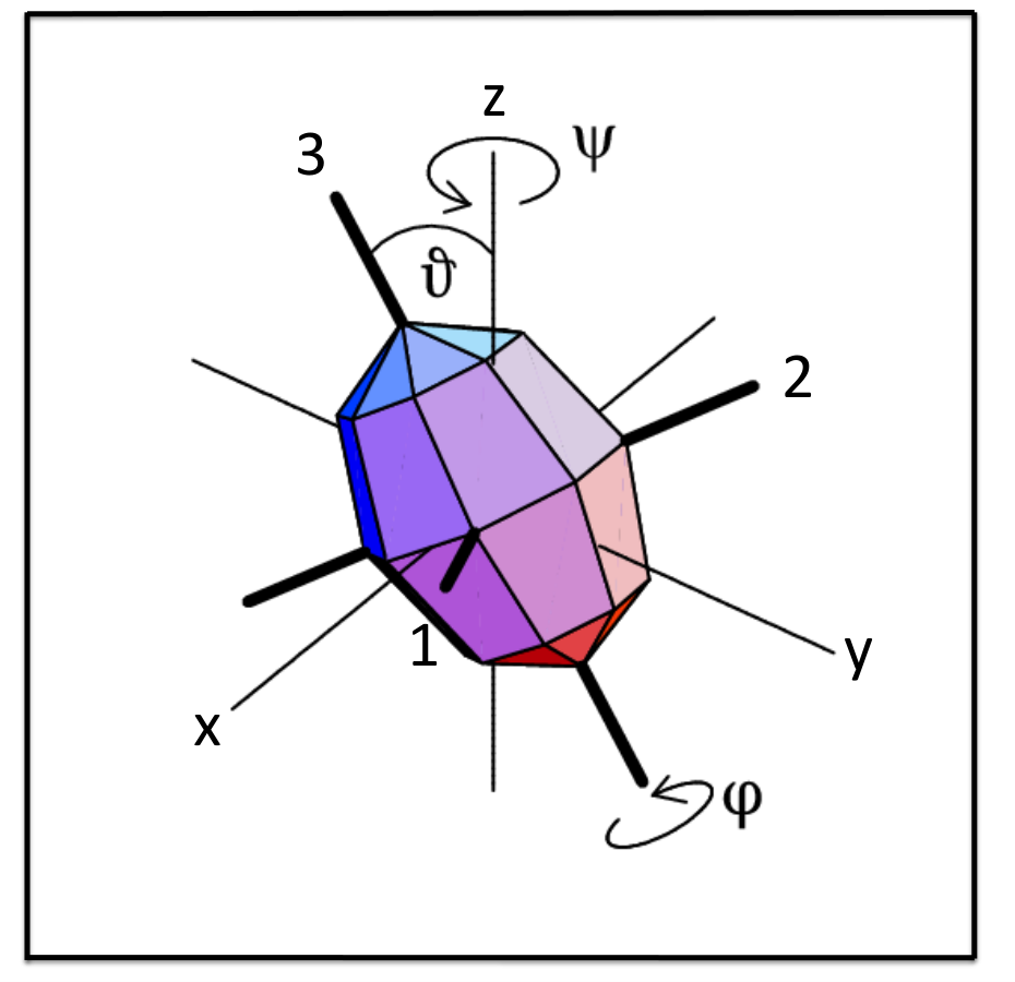
The moments of inertia are parameters that must be determined by additional considerations. The ratios between the moments of inertia of the three principal axes are assumed to be the ones of irrotational flow
| (27) |
where the scale is adjusted to the experimental energies. The analysis of rotational spectra Allmond and Wood 2017 and microscopic calculations by means of the cranking model Frauendorf 2018b demonstrated that the dependence of moments of inertia on the triaxiality parameter is well accounted for by Eq. (27). In the following we use , , and to denote the short, medium, and long axes of the density distribution.
As an example we show in Fig. 2 the energies of the triaxial rotor with the moments of inertia /MeV, /MeV, /MeV, which was studied in Refs. Frauendorf and Dönau 2014; Shi and Chen 2015.
Classical mechanics of gyroscopes provides a classification of the quantal states. The classical orbits of the angular momentum vector with respect to the body-fixed principal axes are the intersection lines between the sphere of constant angular momentum (1) and the ellipsoid of constant energy (24). The construction of the orbits was discussed in detail in Refs. Frauendorf 2018a; Frauendorf and Dönau 2014. For the triaxial rotor the orbits are given by the two angles and as
| (28) | ||||
The orbits on the unit sphere are determined by the implicit equation
| (29) |
They are shown in Fig. 3 for as an example 22 2 Note that the figure shows the polar angles and relative to the -axis, whereas the plot in Ref. Frauendorf and Dönau 2014 shows the phase space and relative to the -axis.. To connect with spectra in Fig. 2 the quantal energies are taken for and the square of classical angular momentum is replaced by its semiclassical corrected value of . The axes 1, 2, and 3 are associated with , , , respectively. Three-dimensional illustrations of the intersection between the angular momentum sphere and the energy ellipsoid can be found in Classical Mechanics textbooks or more specific for nuclei, e.g., in Ref. Frauendorf and Dönau 2014.
There are two topologically different types of orbits. For low energy they revolve the -axis with the maximal moment of inertia, and for high energy they revolve the -axis with the minimal moment of inertia. The separatrix shown by the dashed line in Fig. 2 divides the two regions. It is the unstable orbit of uniform rotation about the -axis with the intermediate moment of inertia. Its energy is shown by the red dashed line in Fig. 2, where the connected states correspond to classical orbits centered about the -axis (below) and -axis (above). The distance between the orbits is determined by an increase of the action by one unit, which is approximately of the area between two orbits on the cylinder shown in Fig. 3. Because the area shrinks with increasing angular momentum, new orbits are born above and below the separatrix, as seen in Fig. 2.
The lowest states correspond to the orbits that revolve the -axis with the largest moment of inertia. These orbits represent the “wobbling” mode. The name is quite appropriate, because the orbit of the angular momentum with respect to the body-fixed axes coincides with the orbit of the -axis of the density distribution in the laboratory system, where the angular momentum vector stands still. “Wobbling” is used to describe the staggering motion of a thrown baseball or of the swaying motion of the earth axis. For small amplitude the wobbling mode becomes harmonic, that is a precession cone that is generated by two harmonic oscillations in and directions with a phase difference of . Bohr and Mottelson discuss the harmonic limit in Nuclear Structure II Bohr and Mottelson 1975 p.190 ff.
III.1 Root mean square values
As a consequence of the D2 symmetry, the expectation values of the angular momentum components on the intrinsic principal axes are zero. Usually their root mean square expectation values are used to visualize the angular momentum geometry,
| (30) |
where we introduced the density matrix . For the considered case of the triaxial rotor without coupled particles it has the simple form
| (31) |
The amplitudes in the three basis sets are
| (32) | ||||
| (33) | ||||
| (34) |
with the amplitudes obtained from Eq. (26).
Fig. 4 shows the root mean square expectation values (30) for the yrast and one- and two-phonon wobbling excitations of the triaxial rotor. The angular momentum of yrast states is best aligned with the -axis, i.e., . The finite and values manifest the quantum uncertainty of the angular momentum orientation, where because .
The one-phonon state has one unit less aligned with the -axis and the two-phonon state two units less . The ratios and are approximately equal to the lengths of the semi axes of the elliptical orbits on the surface of the unit sphere that revolve the -axis (c.f. the states and in Figs. 7 and 9). This relation becomes only obvious when the geometry of the orbits is taken into account.
III.2 -plots
For , Fig. 5 shows the probability distributions
| (35) |
of the angular momentum projection on the three principal axes, which were used in Refs. Frauendorf and Meng 1996; Peng et al. 2003; Qi et al. 2009a; Chen et al. 2010; Shi and Chen 2015 and called -plots or -distributions by the authors.
The angular momentum of the lowest state is aligned with the -axis, which is displayed by the probabilities in the -basis. Complementary, the amplitudes in the - and -basis are broad. The angular momentum of highest state is aligned with the -axis, as seen by the probabilities in the -basis and the very broad distribution and the alternating phase factor in the -basis 33 3 The state state gives .. As seen in the left column, the angular momentum of state is well aligned with the -axis, which is reflected by the peaks centered at , (c.f. Fig. 6). This distribution reflects the close neighborhood of state to the classical separatrix orbit in Fig. 3, which corresponds to the uniform, yet unstable rotation about the -axis with the intermediate moment of inertia (one could call it also Dzhanibekov orbit). The wobbling about -axis nature of state (c.f. Fig. 3) can be recognized in the -basis as the shift of the strong component from to . The analog holds for the state with respect to the -axis.
The probability distributions have been used in illustrating the angular momentum geometry of the triaxial rotor discussed here Shi and Chen 2015 (see Figs. 6 and 7) and chiral bands Peng et al. 2003; Qi et al. 2009a; Chen et al. 2010. They are quite instructive in case of good alignment with respect to one of the principal axes. They are less instructive when the wave function is delocalized (and possibly oscillates), one sees just a broad distribution.
III.3 -plots
The probability distribution of the discrete states is given by
| (36) | ||||
| (37) |
where is angle with the -axis in the --plane and the amplitudes are given by Eq. (6). Fig. 6 shows the same states displayed in the -plots, where it retains the information about the phase factors by showing open and full symbols for or .
The localization of the zero- and one-phonon wobbling states and is well displayed in the -basis as the peaks around . The vibrational character of the state is seen as the zeros at . The discrete distribution of the state is counter intuitive. As is almost a good quantum number (c.f. Figs. 3 and 5), the probability for all ought to be about the same. Instead a decrease toward is seen. It is caused by the symmetrization of the state, , which causes an interference between the states. The density of the squeezed states looks like expected. It oscillates in terms of while the envelop is roughly constant.
III.4 Spin Coherent State (SCS) maps
A new elucidating visualization is to map probability distribution of the SCS. Such SCS maps have first been produced for the two-particle triaxial rotor model in order to illustrate the chiral geometry Frauendorf and Qi 2015. Later the authors of Ref. Chen et al. 2017 used SCS maps, which they called “azimuthal plots”, to visualize the appearance of chiral geometry in the results of quantal calculations in the framework of the angular momentum projection (AMP) method and in the two-particle triaxial rotor model Chen and Meng 2018. In Ref. Streck et al. 2018, the azimuthal plots were first used to study the wobbling geometry. In this section we demonstrate the potential of the method to extract the classical mechanics underpinning of the quantal triaxial rotor model from the numerical results.


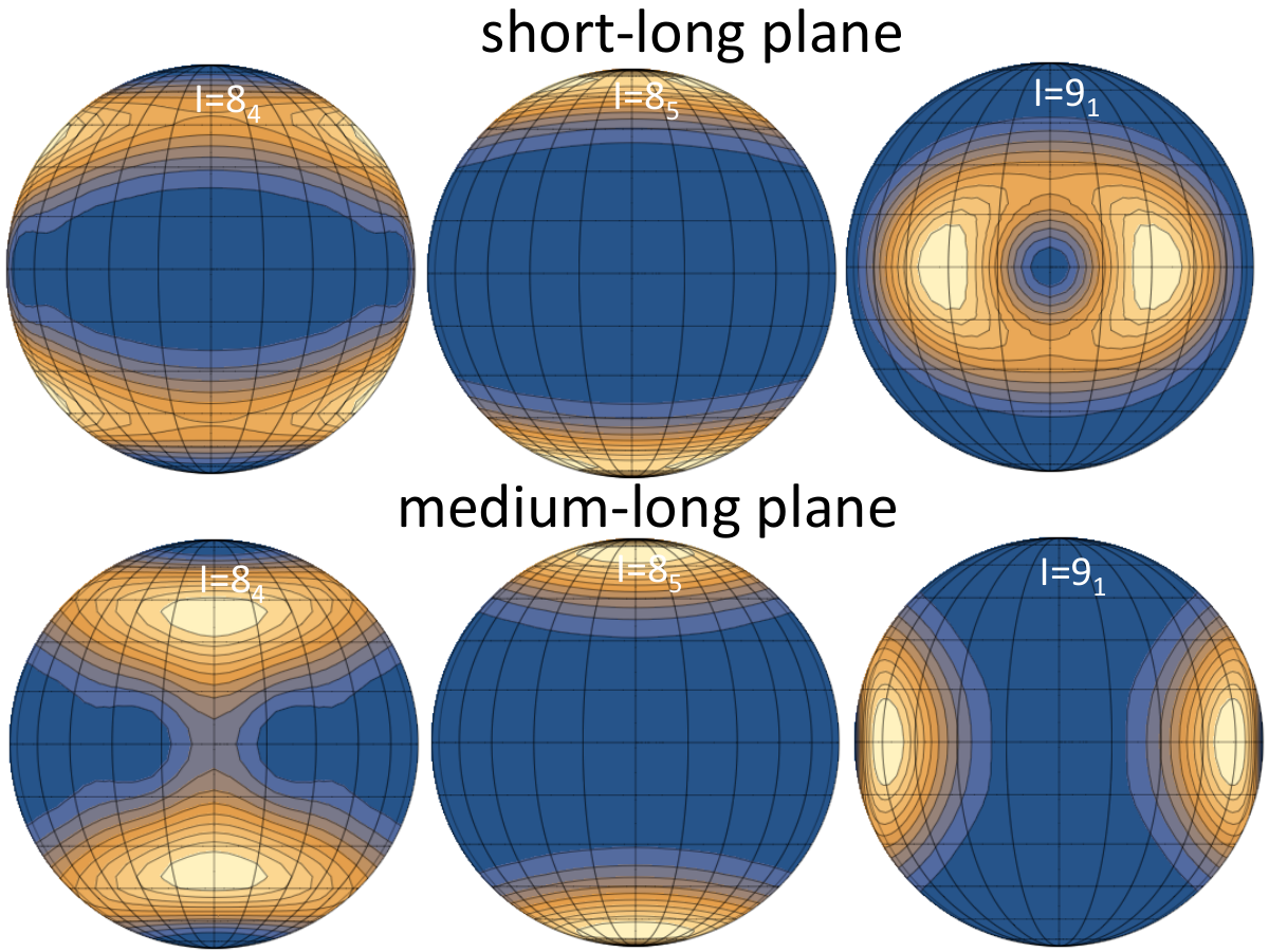
The rotor states in the SCS basis are
| (39) |
Their probability distributions are
| (40) | ||||
| (41) |
Fig. 7 shows contour plots of the probability distributions for the five rotor states and the first state, which we call SCS maps. Note, the maps shown in Refs. Frauendorf and Qi 2015; Chen et al. 2017; Chen and Meng 2018; Streck et al. 2018 do not contain the scale factor of the surface element on the unit sphere. We include it to ensure that the integral (41) is equal to one, and is the probability density on the cylindrical projection.
Preparing a SCS map, one has to decide how to project the surface of the sphere of constant angular momentum onto the map, which is analog to displaying the topography of the earth. Figs. 7 and 8 use the equidistant cylinder projection (invented by Marinus of Tyre 100 AD). Fig. 9 re-displays three of the states using the orthographic projections on the --plane, where the view point lies on the -axis on infinite distance, and the orthographic projections on the --plane, where the view point lies on the -axis at infinite distance (invented by Hipparchos 200 AD). In the orthographic projection is the probability for the SCS to be located in the small trapezoidal patch delineated by the coordinate lines.
The SCS are eigenstates of the angular momentum projection on the --axis,
| (42) |
where the axes are assigned as 3-, 1-, 2-. That is, Figs. 7, 8, and 9 show the probability for the angular momentum being oriented in a specific direction with respect to the principal axes of the body-fixed frame. However, “oriented” has to be understood in a restricted sense. The orientation is only specified within a distribution with the width discussed in the context of Eq. (17). We illustrate the uncertainty of the orientation as a green circle with the radius . In other words, the SCS maps are blurred by the Uncertainty Principle like a poorly resolved picture of the Earth’s surface taken from large distance (Zoom out Google Earth).
III.4.1 Ridges and classical orbits
The full lines in Figs. 7 and 8 depict the classical orbits from Fig. 3 for the angular momentum and the quantal energies as given in Fig. 2. The ridges of the SCS probability density distributions trace the corresponding classical orbits, that is, the SCS distribution is a fuzzy reproduction of the classical orbit. Note, the close correspondence between the ridges and the classical orbits appears only when the geometric scale factor is included in . The SCS maps filter out the classical mechanics underpinning of the quantal TRM with the best resolution permitted by the Uncertainty Principle.
The exact location of a ridge is found by determining the minimum of the square of the gradient as function of for given or as function of for given . Alternatively, one may search for the maximal curvature 44 4 The curvature of the contour line is given by , where , denote first order and , , second order partial derivatives. The expression holds when the contour line is a single-valued function . In case it is a single-valued function the curvature is . of the contour line. In principle, the two methods ought to give the same result 55 5 Approximate the region near the tong tip of a contour by an ellipse. The tip is located at the long semi axis where the curvature is maximal and distance to a slightly larger ellipse that approximates a nearby contour is maximal.. However, the equivalence holds only for infinitesimal distances. Approximating derivatives by finite differences on a grid of 1 degree, we found slight differences that are not visible on the scale of the figures.
As an example, Fig. 10 shows the ridge for the state determined numerically in this way. The SCS map filters the corresponding classical orbits from the quantal state as the location of the ridge. Although being close, the ridges deviate somewhat from the classical orbits with energy equal to the quantal energy of the rotor. As seen in Fig. 10 the classical orbit with the energy comes very close to the numerical determined ridge. The deviations are caused by the symmetrization of the quantal wave function, which couples the two distinct classical orbits.

As seen in Fig. 7, the ridge of the state is somewhat smaller than the classical orbit, because the state contains only the components =8, 6, 4, 2. The classical orbit also contains the projection , which has a larger distance from the center. For the 82 state, the ridge is closer to the classical orbit because the wave function contains the =8 component with . The turning points 2 and 4 of the ridge are somewhat closer to the center than the ones of the classical orbit. This is caused by the interaction with the turning points of the backside orbit (centered at ), which is seen as the bridges that connect them through , .
III.4.2 Velocity and phase
Janssen Janssen 1977 has shown that the expectation values obey the Euler equations which govern the classical motion of the triaxial top 66 6 This is a special case of the time development of coherent states being governed by the classical equations of motion.. This suggests an extension of the interpretation in classical terms: the scale of the SCS probability density represents the fraction of the period time that the rotor stays in a section of the orbit.
The probability to be in a square that encloses and has the edges parallel to the ridge to and perpendicular to it is given by
| (43) |
Classically, the probability to be in the interval of the orbit that encloses is given by
| (44) |
where is the angular velocity tangential to the orbit and the period. That is, if the SCS states obey the classical equations of motion, the probability of the SCS to be in the interval perpendicular to the ridge top is
| (45) |
which means . The classical angular velocity tangential to the orbit is
| (46) | ||||
| (47) | ||||
| (48) |
where and are given by Eq. (29). The result of is obtained from the fact that the angles satisfy Euler’s differential equations.
Fig. 11 compares the classical angular velocity for the two orbits shown in Fig. 10 with the scaled inverse probability density along the numerically determined top of the ridge shown in Fig. 10. The inverse of the probability density well approximates the angular velocity of the classical orbit that comes closest to the ridge top. The deviations near the turning point reflect the deviation of the classical orbit from the ridge top seen in Fig. 10.

The phase difference relative to some chosen point (only relative phases have a physical meaning), is given by
| (49) |
Conservation of flux relates the phase of the wave function to its probability density . For the SCS maps the conservation implies that is constant, where the integral is taken perpendicularly across the fuzzy orbit. That is, when goes down must go up. Therefore the phase change can be estimated from the probability density in a qualitative way. As is the momentum density in direction of the orbit, its connection with just tells us that the rotor passes the regions of low density faster than regions of high density, which repeats the above discussed interpretation of the inverse of the probability density as the tangential angular velocity.

Semiclassically, the phase is the mechanical action in units of , that is
| (50) |
if is in units of as commonly assumed. For the state , Fig. 12 compares the classical phase difference (50) with the SCS phase difference (III.4.2) along the path on top of the ridge. The latter nearly agrees with the classical phase of the orbit that come closest to the ridge in Fig. 10. That is, one can estimate the phase from the SCS map in orthographic projection (like Fig. 9) as the area between the meridians and multiplied by .

Fig. 13 displays the phase differences for the complete orbits of the states 91, 82, and 83. The function in Eq. (III.4.2) jumps from to at its branch cut. This generates the jumps of the full curves in the figure. The phase is only determined up to a multiple of . The dashed curves are generated by adding to the full curve such that a continuous curve results, which represents the increment of the action along the path. The jumps make two-dimensional maps of the phase generated by means of Eq. (III.4.2) very complex. We did not find them useful for interpretation. A calculation of the phase along the orbit (ridge of the probability density) provides useful insight in the quantal nature of the state. Semiclassical quantization requires that the classical action for a full turn must be . The number of phase jumps in a figure like Fig. 13 provides such kind of quantum number for the angular momentum motion.
The phase gain after passing one turn of the periodic orbit is of topological nature. We checked numerically that any closed path in the SCS plane of a state which encloses , gives a phase gain of respectively . This holds not only for the wobbling states but also for the states above the separatrix, which revolve the poles .
III.4.3 Detailed discussions of the SCS maps
Now we discuss the SCS maps in Fig. 7 in more detail. The yrast state 81 represents uniform rotation about the -axis. Accordingly the probability distribution is a blob centered at . Because of the D2 symmetry being even with respect to a rotation by about the three principal axes, there is another blob at . The doubling caused by the D2 symmetry is present in all other SCS maps.
The states and 82 are, respectively, the one- and two-phonon wobbling excitations about the -axis. Accordingly, their probability distributions are fuzzy ellipses centered at the -axis, where the size of the two-phonon 82 ellipse is larger. The probability is highest at the two turning points 2 and 4 of the coordinate , where classically the angular velocity is zero, and it is the lowest at the two turning points 1 and 3 of where the angular velocity has a maximum. For the one-phonon state the phase calculated by means of Eq. (III.4.2) is , , , at the turning points 1-4, respectively. For the two-phonon state the phase is , , , at the turning points 1-4, respectively. The phase increment corresponds to the action increment along the classical orbit, which is used for semiclassical quantization (see Fig. 13 and Ref. Frauendorf and Dönau 2014). As expected, the one-phonon wobbling state is odd and the two-phonon state even under .
The state is close to the classical separatrix orbit in Fig. 3. The separatrix contains the stationary points , and , , for which the rotor rotates uniformly about the -axis. These stationary points are unstable with respect to the dashed orbits, where it takes infinite time to approach or leave the stationary point. Accordingly, the SCS probability is centered around the -axis, and it has four extrusions in direction of the separatrix branches. As seen in Figs. 3 and 7, the classical orbit with its quantal energy lies slightly outside the separatrix. That is, it revolves the 3-axis (-), and it is topologically different from the so far discussed states, which revolve the 2-axis (-). This is reflected in Fig. 13 which shows a steady increase of the phase difference from , where to , where . The phase increment is small near at the points 2 and 4 and large only a little away from them. That is, the angular velocity is, respectively, small near and large away from these points. In terms of classical motion this means the rotor stays for a certain time rotating about the -axis, then it quickly flips to opposite direction of the -axis, remains for the same time rotating about it, then it flips back, etc. We suggest the name axis-flip wobbling for this flipping motion, which is repeated periodically. For macroscopic objects it is called the Dzhanibekov effect after the Russian astronaut, who unscrewed a wing nut under zero gravity, which slipped his hand and executed the axis-flip motion while flying through the space station. The reader can watch it on an entertaining movie on 77 7 https://www.youtube.com/watch?v=L2o9eBl_Gzw.. A recent mathematical analyse has been published in Ref. Mardešić et al. 2020, where further references can be found.
For odd the D2 symmetry requires that the wave function is odd with respect to a rotation about the -axis by . This is only possible if it is zero on the -axis, which is seen as the hole in the distributions for the states , , and . The acceleration away from the -axis increases with the distance from it. Due to the presence of the hole, the rotor remains a shorter fraction of the total period in this position than for even , which means it spends a larger fraction on the flip orbit.
As seen in Fig. 2, the energy difference between axis-flip states of even and odd is much smaller than the wobbling energy between two adjacent harmonic oscillation (HO) multi-phonon states. The transition from the HO limit to the axis-flip regime is gradual. The distance between adjacent states of opposite signature decreases. The fraction of the period the rotor stays near the -turning points increases.
The angular momentum of the state is as far as possible aligned with the -axis. Accordingly, the SCS probability density is maximal for and depends weakly on . The state has two-phonon structure with respect to the -axis. The polar angle and , and the azimuthal angle revolves the -axis.
The SCS plots disentangle the states that are superposed to generate the D2 symmetry. They appear at different places in the map. The pertaining classical orbits revolve the respective axis in opposite direction. This is clear from the orientation of the constituent SCS with respect to the axis and is reflected by the opposite sign of the phase calculated by Eq. (III.4.2).
Using the symmetry properties of D-function, Eq. (39) can be rewritten as
| (51) | ||||
| (52) |
As describes the orientation of the body-fixed axes in the laboratory frame, one recognizes that the SCS map also shows the probability for the rotor (its body-fixed axes) being oriented with respect to the laboratory frame. The two perspectives represent the “active” rotation of the state vectors generating the SCS basis versus the “passive” rotation of the coordinate system.
The panels , , and display, respectively, for the zero-, one-, and two-phonon states the wobbling motion of the -axis about the -axis of the laboratory system, along which the angular momentum is aligned. The state lies energetically quite close to the separatrix in Fig. 3. The panel shows that it corresponds to rotation about the unstable -axis with low probability to move away. The states and correspond to precession of the -axis about the laboratory -axis. (Fig. 9 is quite helpful in realizing the different types of shape wobbling.)

III.5 Transition density maps
The SCS probability density maps lose the information about the phase, which has to be exposed separately. Another way to retain this information is to map the transition density. It is well known from textbooks that the electromagnetic transition probabilities can be obtained from the classical radiation power by replacing the classical expression for the oscillating multipole by its the integral over the transition density obtained from the wave functions of the initial and final states (e.g., Ref. Krane 1988). Reversing the perspective, a SCS map of the transition density filters out the oscillating multipole that generates the transition.
The interband transition probability is calculated as
| (53) |
The matrix element is
| (54) |
with the quadrupole moment operator
| (55) |
We can define the transition density matrix as
| (56) |
and define the transition SCS plot as
| (57) |
The transition matrix element becomes an integral over the transition density and the quadrupole operator,
| (58) |
In classical radiation theory the matrix element (III.5) is replaced by the corresponding integral, which contains the time-dependent charge density instead of the transition density. That is the SCS map of the transition density visualizes the corresponding classical motion of the charge density.
Fig. 14 illustrates the transition from the one-phonon wobbling state to the zero-phonon state . The upper panels show the SCS maps of the transition density. The two blobs with opposite sign of the real part represent a linear oscillation of the body in -direction and the two blobs of the imaginary part a linear oscillation in -direction. The two linear oscillation with a relative phase shift of combine to an elliptical wobbling motion, which is shown by the absolute value in the middle panel. Multiplying the motion of the charged body by the quadrupole operator in the right middle panel, gives the integral of the matrix element (III.5). As the quadrupole matrix element is real, the integral over the imaginary part (lower left panel) is zero, as can easily be seen from its anti-symmetry. Only the integral over the real part is left.
IV Particle triaxial rotor model
Transverse and longitudinal wobbling as well as chiral modes are described by coupling particle(s) to the triaxial rotor, which leads to increasing complexity of the wave function. In order to visualize the angular momentum constituents of interest the reduced density matrix is used, which is constructed by averaging over the degrees of freedom that are not of interest. In this section we discuss the particle-plus-triaxial rotor model (PTR), which couples one high- particle (hole) to the triaxial rotor core. In his seminal papers Meyer-Ter-Vehn 1975a; Meyer-Ter-Vehn 1975b, Meyer-ter-Vehn generalized the approach to the quasiparticle triaxial rotor model and demonstrated its impressive capability to account for the experimental data in odd- nuclei available at the time. He interpreted the numerical results in the framework of a weak coupling approach. Here we focus on the analogies with classical mechanics of gyroscopes. In particular, the concepts of transverse and longitudinal wobbling introduced by Frauendorf and Dönau Frauendorf and Dönau 2014 will be substantiated by means of the various ways to analyse the quantal numerical results, which have been introduced in the preceding section.
IV.1 Construction of the plots
The PTR couples a high- particle to the triaxial rotor core. The corresponding Hamiltonian is
| (59) | ||||
| (60) |
where is the total angular momentum, the angular momentum of the particle, the angular momentum of the triaxial rotor, and is the coupling strength to the deformed potential.
The PTR Hamiltonian is diagonalized in the product basis , where are the rotational states for half-integer and the high- particle states in good spin approximation. The eigenstates are
| (61) |
The coefficients of the states in the triaxially deformed odd- nuclei are not completely free. They are restricted by requirement that collective rotor states must be symmetric representations of the D2 point group: When the and in the sum run respectively from to and from to , their difference must be even and one half of all coefficients is fixed by the relation .
From the amplitudes of the eigenstates , the reduced density matrices
| (62) |
and
| (63) |
are obtained, which contain the information about the particle angular momentum and the total angular momentum , respectively.
Most commonly discussed quantities (e.g., in Refs. Qi et al. 2009a; Qi et al. 2009b; Chen et al. 2010; Hamamoto 2013; Zhang and Chen 2016; Chen and Meng 2018; Streck et al. 2018; Chen et al. 2019b; Chen et al. 2019; Chen et al. 2020; Chen et al. 2020) are the root mean square expectation values of the projections on the principal axes the rotor of the total angular momentum , the proton angular momentum and the collective rotor angular momentum ,
| (64) | ||||
| (65) | ||||
| (66) |
One may define orientation angles of the classical vectors defined by means of the root mean square expectation values of the angular momentum components. Another way to derive mutual orientation angles from PTR wave functions has been introduced in Refs. Starosta et al. 2002; Tonev et al. 2007. It consists of replacing the classical expression for the angle derived from vector products by the corresponding quantal operator expression. For example the angle between and the replacement is
| (67) |
The -plots Qi et al. 2009a show the probability distribution with respect to three principal axes which are for the total angular momentum
| (68) | ||||
| (69) | ||||
| (70) |
and the proton angular momentum
| (71) | ||||
| (72) | ||||
| (73) |
Alternatively, the probability distributions for the - and -axes can be calculated by the simple expression for the -axis and re-assigning the axes by changing and . Fig. 26 shows the -plots for selected yrast and wobbling states.
The SCS map for the total angular momentum is given by Eq. (40) using the density matrix (63). For the particle angular momentum the map is given by
| (74) |
with the density matrix (62). Fig. 23 shows the SCS maps in cylindric projection for the total angular momentum, which are calculated by means of Eq. (40) using the density matrix (63). Fig. 22 adds a selection of the SCS maps in orthographic projection. Figs. 24 and 39 show the SCS maps for the odd proton in cylindrical projection.
The phase changes between different angles of is given by Eq. (III.4.2) with reduced density matrix using (63). It is important to realize that the reduced density matrix implies a certain degree of decoherence. The full density matrix (31) of the TRM represents one quantal state, which has fully coherent phase relations between different angles. In this case the phase differences are additive: . For the reduced density matrix this holds only approximately in case of weak decoherence or gets completely lost.
SCS plots of the transition density are obtained by means of Eq. (III.5) using the reduced transition density matrix (63). The more detailed behavior of the core angular momentum is visualized by the () and plots introduced in Refs. Streck et al. 2018; Chen et al. 2019b. The basis of the PTR eigenstates is re-coupled,
| (75) |
with
| (76) |
and a density matrix matrix is obtained from the components in the new basis
| (77) |
The probability distribution for the projection on the 3-axis is given by
| (78) |
The distributions with respect to the 1- and 2-axes are obtained by means of changing and . In contrast to and the absolute value of core angular momentum is not constant. Its probability distribution is given by
| (79) |
The SCS map showing the orientation of the core angular momentum with respect to the body-fixed coordinate system is constructed as
| (80) |
and the distribution
| (81) |
shows the probability for the orientation of rotor angular momentum , where its length depends on the angles.
We discuss the interpretation of the PTR model using 135Pr studied in Refs. Frauendorf and Dönau 2014; Streck et al. 2018 as an example. The parameters of the PTR are (corresponds to ), , and , 13, . Fig. 15 shows the energies of the lowest bands, which represent the zero-, one-, two-, and three-phonon wobbling states and the lowest excitation of the particle mode (signature partner state). Fig. 16 displays the standard angular momentum alignment Bengtsson and Frauendorf 1979 relative to a Harris reference, which corresponds to uniform rotation about the -axis.
IV.2 Geometry of the PTR states — the classical limit
The classical analog to the quantal PTR corresponds to considering and as pairs of classical canonical variables, which means, in Eq. (2) the commutator is replaced by the Poisson bracket. The classical PTR Hamiltonian is
| (82) | ||||
| (83) |
with angular momentum projections on --plane and . Using the classical Hamiltonian, we replace and , which is a semiclassical correction that brings the classical results closer to the quantal ones.
The system is two-dimensional and non-separable, that is, one cannot construct the orbits by conservation laws as for the TRM. Solving the classical equations of motion
| (84) |
is by far more complicated than finding the quantal states. Most relevant for the interpretation of the latter is the topological classification of the classical motion.
The static equilibrium configuration is found by minimizing with respect to all four angles, which gives the classical correspondence of the yrast energy. The minimum lies at and at the and values shown in Fig. 17.


The location of the minimum as function of angular momentum is understood as follows. The triaxial rotor is coupled with an proton. The -axis is its preferred orientation, because it maximizes the overlap of the particle orbit with the triaxial core Frauendorf and Meng 1996. The rotational energy of the rotor core prefers the -axis with the largest moment of inertia. Fig. 17 shows the result of the two competing torques. At low the torque of the quasiparticle wins. The orientation of and along the -axis represents the stable configuration. The growth of total angular momentum is generated by an increase the core angular momentum along the -axis. Above the critical angular momentum the torque of the rotor core takes over. The energy minimum moves to the angle in the --plane. The growth of total angular momentum is essentially generated by an increase the core angular momentum along the -axis while the components stays constant. The particle angular momentum is pulled toward to -axis because the Coriolis force tries to minimize the angle between and . The root mean square angular momentum components shown in Fig. 18 reflect the position of the classical energy minimum.
The development of the angular momentum geometry with increasing spin has already been discussed in Ref. Frauendorf and Dönau 2014. In order to simplify, the authors assumed that the angular momentum of the particle is rigidly aligned with the -axis (frozen alignment approximation-FA). At low the rotor angular momentum aligns with the -axis, in this way minimizing the Coriolis force. For rotor angular momentum re-aligns toward the -axis, which has the largest moment of inertia 88 8 For a detailed discussion of the coupling high- orbitals with the rotating triaxial potential see Ref. Frauendorf 2018a.. The critical angular momentum of in Fig. 17 is lower than the FA estimate of in Ref. Frauendorf and Dönau 2014 because taking into account the finite de-alignment of the proton lowers the stability of the minimum at .
The orientation angles can also be determined by applying the tilted axis cranking (TAC) approximation to the PTR Hamiltonian. In this case only the total angular momentum operator is replaced by its classical vector and the reduced PTR Hamiltonian is diagonalized in the subspace of the odd particle. The resulting energy is minimized with respect to the orientation angles , of the total angular momentum. The resulting angles are shown in Fig. 17 and corresponding angular momentum components in Fig. 19 together with their values at the minimum of the classical energy. For comparison, the root mean square components , , , , are included in Fig. 19. The cranking angular momentum components are not far from the classical values as expected from the angles shown in Fig. 17. The root mean square angular momentum components of the yrast states behave roughly like their cranking and classical counterparts. The contributions of the fluctuations to the root mean squares wash out the characteristic kinks at the critical angular momentum and generate 1-2 units of angular momentum for the vanishing components.
Fig. 20 shows the angle between the proton angular momentum and the total angular momentum . In case of the angles calculated by minimizing the classical yrast energy, shown in Fig. 17, which is zero below and increases afterwards. The angles obtained by the classic vector expression (67) from the root mean squares of the angular momentum components of the yrast states increase steadily. They approach the angles at the minimum of the classical energy at large , whereas the kink at is washed out. The quantal expectation value of the operator scalar product (67) gives a nearly constant angle, which is substantially larger than the angles obtained from the root means square values of the angular momentum components. The quantal indeterminacy of the angular momentum components leads to severe deviations from the classical vector scheme. The angles determined this way do not well reveal the underpinning angular momentum geometry.
A topological classification can be found by considering the adiabatic energy , which is obtained by minimizing classical energy with respect to the angles , for fixed angles , . The adiabatic energy along the path is displayed in Fig. 21, which represents the bottom of the valley in the surface . The figure includes the quantal PTR energies from Fig. 15 relative to the minimum of . The additional energy of the PTR states can be assigned to the collective wobbling motion. Assuming a constant mass parameter for the degree of freedom, the classical orbit is confined to the range . As will be discussed in detail below, the character of the PTR wave function is closely related to the classical orbit. There are three topological regions.
- 1.
Transverse wobbling (TW, panel ): the total angular momentum oscillates around , , which is the -axis that is transverse to the -axis with the largest moment of inertia.
- 2.
Longitudinal wobbling (LW, panel ): the total angular momentum oscillates around , which is the -axis with the largest moment of inertia.
- 3.
Axis-flip wobbling (panel ): the total angular momentum jumps over the whole range of .
The TW and LW modes are restricted to the lowest states. For the higher states the total angular momentum de-localizes.
IV.3 Transverse wobbling
The authors of Ref. Frauendorf and Dönau 2014 classified the excited wobbling states of the PTR system. In order to introduce the classification scheme, they started with assumption that odd quasiparticle is either rigidly aligned with the - or -axis, which are transverse to the -axis with the largest moment of inertia (transverse wobbling TW), or that it is aligned with the -axis (longitudinal wobbling LW). The assumption of “frozen alignment” FA makes the problem one-dimensional and the angular momentum orbits are the intersection lines of the angular momentum sphere and the energy ellipsoid, the center of which is shifted from origin Frauendorf and Dönau 2014. For the TW regime the revolves the -axis if the quasiparticle is particle-like or the -axis if it is hole-like. For the LW regime revolves the -axis. The classification of TW-LW was introduced in Ref. Frauendorf and Dönau 2014 based on the FA assumption because it leads to a transparent picture in terms of the classical orbits and to simple analytical expressions for the energy and transition in the small amplitude limit, the harmonic frozen alignment (HFA) approximation. Although not explicitly stated, the TW classification was understood in the topological sense illustrated by Fig. 21: the total angular momentum oscillates around the -axis, which is transverse to the -axis. Classically, the yrast states represent uniform rotation about the transverse -axis. For the TW excitations revolves the -axis in the body-fixed frame and in the laboratory system the density distribution wobbles such the -axis executes an ellipse with respect to the angular momentum axis . Fig. 17 shows that in TW regime, the classical vector is aligned with the -axis. As seen in Fig. 19 the alignment of in the yrast states is not complete for the full quantal calculation. As expected, the -component is smaller and the -component larger for TW excitation than for the adjacent yrast states.

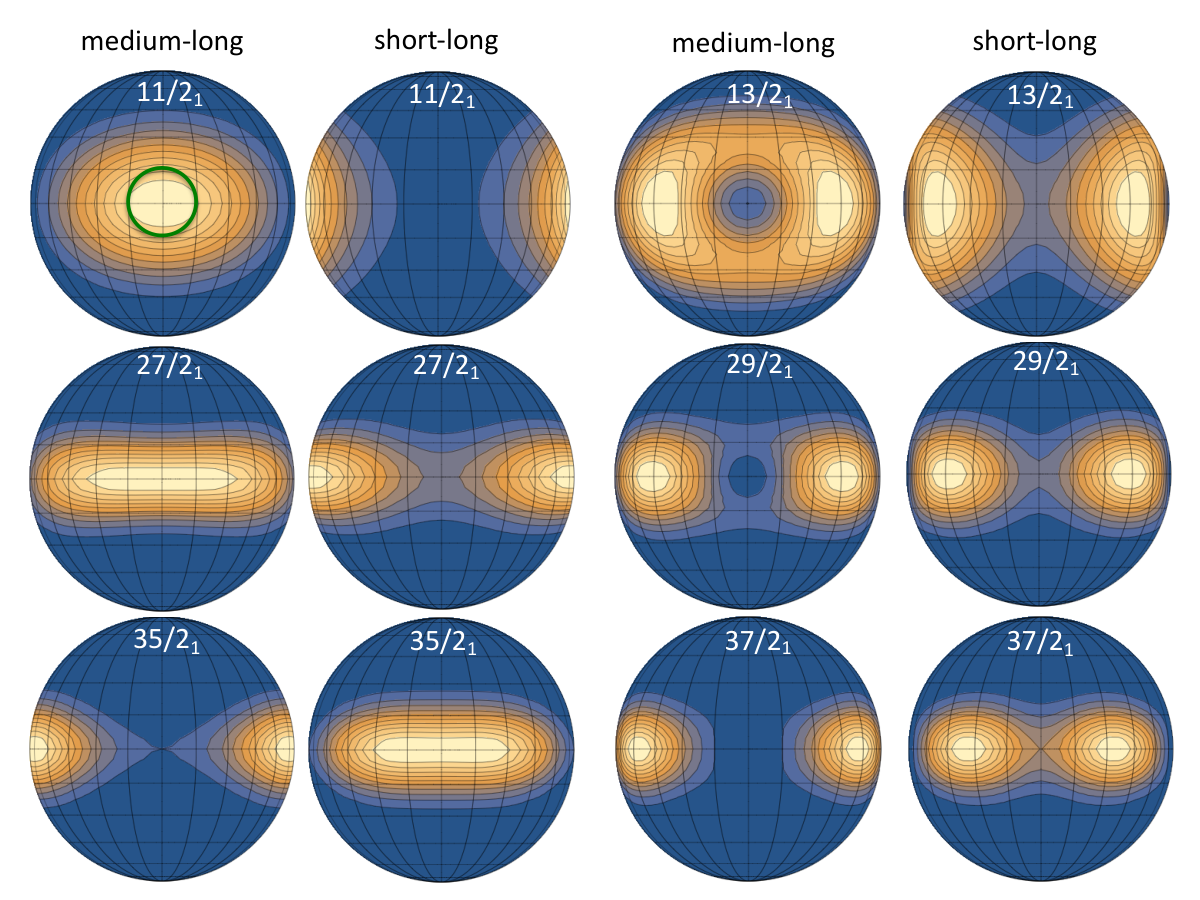
The SCS maps, which are directly generated from the quantal results, clearly illustrate the topology. Figs. 22 and 23 show the maps for the total angular momentum obtained by Eq. (40) using the density matrix (63). The TW regime extends to the critical angular momentum . The probability in the yrast maps , (not shown), and is localized around the -axis. The maps , (not shown), and for the one-phonon states show a rim that revolves the -axis. The distribution is analog to one of the one-phonon states of the simple rotor in Fig. 7, which has a rim around the -axis.
The dots in Fig. 23 display the minima of the classical energy given by the angles and according to Fig. 17. The SCS maps include the classical orbits, which are the contours of the adiabatic classical energy . As discussed in context with Fig. 21, the TAC energy at the minimum contains the zero point energy of the proton. The additional PTR energy is assigned to the wobbling motion.
The classical orbits trace the rim, although not quite as close as in the case of the simple rotor. Fig. 24 displays the probability distribution of of the odd proton obtained by Eq. (74) for the state . As expected for the TW regime, the density distribution is centered at the -axis. The distribution is wider than the natural width of the SCS, which is indicated by the circle. This reflects the zero point fluctuations of . The -maps for the states and are nearly the same, as expected for the strong coupling of the proton.
Fig. 25 shows the phase increment along the classical orbit of the one-phonon TW state . The phase development is similar to the triaxial rotor (TR) one-phonon wobbling state in Fig. 13. The phase gains over one revolution. However, the phase gain over the four branches between the turning points in not symmetric as in Fig. 13. The origin has been mentioned before. The phase is calculated from the reduced density matrix, not from the complete density matrix as for the TR state . The reduction generates some loss of phase information, which has the consequence that phase increment is no longer additive. The phase increment in Fig. 25 is calculated relative to the turning point at in the upper branch of the classical orbit. Relative to this starting point the lower branch differs from the upper one, and so does the phase increment. Nevertheless, the total gain after one revolution is , as expected.
The -plots in Fig. 26 qualitatively agree with the distributions along the three axes in the SCS maps, which is best visible by comparing with the maps in the orthographic projection Fig. 22. The existence of the rim around the -axis in Fig. 23 can be guessed from inspecting the -plots for the three axes.
Fig. 27 shows the SCS maps of the total angular momentum for the second and third wobbling states. In a harmonic vibration scenario, the two-phonon states and should appear as a wobbling mode with a wider rim than the one-phonon states (c.f. the state in Fig. 7), which is the case (c.f. in Fig. 23). However the wobbling cone that revolves the positive -axis and the cone that revolves the negative -axis are no longer as well separated as for the one- and zero-phonon states, which is expected from inspecting Fig. 21. The overlap causes deviations from the harmonic regime. Analogous to the state of the TR, the merging of the rims at indicates the instability of the TW mode. The anharmonicities drive the TW wobbler toward the axis-flip regime like in the case of the simple TR discussed in Sec. III.4.3. The role of the axes is reversed. In the TW regime the -axis is the stable and -axis the unstable axis. The concentration of the probability near the -axis signals the approach to instability of the TW mode. The -distributions in the lower two rows of Fig. 24 show the weak reaction of the proton angular momentum caused by the Coriolis coupling with . The distribution becomes elongated toward the -axis.
The -distributions of the and states have bridges at , between the upper and lower parts of the rim. They are a quantum feature. The state of the one-dimensional harmonic oscillator has probability distributions and , which are determined by the Hermite polynomial . The polynomial has a maximum at and , respectively. The corresponding bumps can by seen in the and in Fig. 26. The bumps combine to the bridge in the two-dimensional SCS map. We will discuss the structure in more detail in Sec. IV.4. The bridge is less visible for the TR two-phonon state in Fig. 7. The reason is the presence of the proton, which pulls toward .
Fig. 21 shows that the structures are not well confined by the classical potential. The map for the states in Fig. 27 and (not shown, but looks alike) have axis-flip character as well. Their probability around , is very small, because the state is odd under . The -map for the state is complex. We attribute this to the admixture of the signature partner structure, which has maxima at , (see discussions in the next section). The -distributions of the states in Fig. 24 show some response of the proton angular momentum to the inertial forces.
IV.4 Transverse wobbling and signature partner modes
For angular momentum well below the instability at the amplitudes of and are small, which allows one to approximate the PTR as a system of two coupled harmonic oscillators. As the coupling is not very strong in the TW regime, one may classify the excitations in terms of individual excitations of the uncoupled modes. The harmonic approximation has been worked out in Refs. Tanabe and Sugawara-Tanabe 2017; Raduta et al. 2020. The authors applied boson expansions to the angular momentum operators. The leading terms provide the coupled oscillator approximation. A review of the work in Ref. Tanabe and Sugawara-Tanabe 2017 is given in the Appendix A.
Here we discuss the structure of the two-oscillator Hamiltonian. We derive it in a modified way, which was used in Ref. Frauendorf and Dönau 2014. Assuming that amplitudes of , , , are small one may approximate
| (85) | ||||
| (86) |
and the PTR Hamiltonian (59) by the bi-linear expression
| (87) |
With the term
| (88) |
is recognized as the HFA Hamiltonian introduced in Ref. Frauendorf and Dönau 2014, which generates the pure harmonic TW excitation spectrum. Analytical expressions for the energies and transition probabilities are given there.
The modified particle Hamiltonian
| (89) |
has the form of a Hamiltonian in a frame rotating with the angular velocity . The cranking term accounts for the inertial forces. The other two corrections are known as the “recoil terms” of the PTR. As the particle excitations are given by the states in the rotating potential, the authors of Ref. Ødegård et al. 2001 called them “cranking mode”. We will keep this name. Interpreting the spectra in the framework of the Cranked Shell Model, it has become customary to call “signature partner” the excited quasiparticle Routhian of opposite signature which branches from the yrast Routhian with increasing . The authors of Ref. Matta et al. 2015 kept the custom using the name “signature partner band”. In the following we will also use the name “signature partner” to denote the first excited state of the odd proton. It should be noted that the authors of Ref. Tanabe and Sugawara-Tanabe 2017 called the cranking mode “precessional mode” and the authors of Ref. Raduta et al. 2020 use the terminologies “transversal”, “longitudinal”, and “signature partner” in different ways, which may cause confusion.
The term
| (90) |
couples the wobbling and cranking modes.
As reviewed in the Appendix A, the authors of Ref. Tanabe and Sugawara-Tanabe 2017 derived a somewhat more accurate expression for by means of Holstein-Primakoff boson expansion of the angular momentum operators, which includes semiclassical correction terms. After mapping on the boson space, it is diagonalized by means of a Bogoliubov transformation for bosons. The eigenvalue equation has two real solutions: the lower wobbling and the higher cranking solution. They are shown in Fig. 28 where they are labeled as HO , 2, 3 and SP, according to their character. The wobbling mode is unstable for , which is close to the instability of the minimum of the classical energy at in Fig. 17. This instability makes the vanish rapidly. Also shown are the uncoupled wobbling and cranking modes obtained by setting , which corresponds to in Eq. (A). The wobbling mode agrees with the HFA for TW in Ref. Frauendorf and Dönau 2014. (There are slight numerical differences caused by the mentioned semiclassical correction terms.) The FA approximation makes the TW mode more stable. As discussed in context of Fig. 17 the FA moves instability of the minimum of the classical energy at the -axis to higher values.
The slope of the cranking solution for SP is about . This corresponds to the difference of the particle alignment of about between the unfavored and favored signature partners, which is expected from the cranking Eq. (IV.4) and consistent with the alignment results shown in Fig. 16.
Fig. 28 compares the wobbling energies of the exact solutions of PTR with the approximate solutions of HP boson expansion. For , 17/2, PTR solutions agree fairly with the , 2, 3 HO TW phonon excitations. The PTR energy decreases with the increasing spin up to , which is the hallmark of TW. After that the TW regime changes into the transition and further into the LW regime. The HO approximation gives a collapse of TW at , which is near the angular momentum where the -minimum of the classical and TAC energy become unstable (cf. Figs. 17 and 19). The instability appears earlier than the end of the TW regime of exact solutions by PTR.
Fig. 29 compares the - and -distributions of the HO with PTR for . The HO shows the well known pattern generated by the Hermite polynomials of order 0, 1, 2. It is seen both in and ) on a different scale. As discussed in the Appendix A, the distributions are related as , where is the width of , because represent, respectively, the position and momentum operators of the TW oscillations. The narrow -distributions of HO and PTR agree well with each other, although the HO ones are somewhat more narrow. The -distributions deviate from each other substantially. The reason is that the space is finite, . Mapping it on the infinite boson space by means of the HP expansion removes this restriction. The wave function can relax beyond the limits, which lowers its energy and leads to instability eventually.
For the yrast states , , and , PTR and HO agree rather well. For the one-phonon states and , the HO distributions extend beyond the limit, which correlates with the deviation of the PTR energy from the HO value. The PTR distribution has the form of the one-phonon HO distribution cut at the maximal value . The cut-off does not substantially modify SCS plots for these states in Fig. 23, which look as expected for one-phonon states. The SCS map of the state, which is unstable for the HO approximation, deviates noticeably from the harmonic one-phonon shape. This indicates the proximity of the instability of the TW regime, where the classical energy substantially deviates from a parabola.
The PTR distributions for the states , , and deviate strongly from the HO distributions with phonon number . For small both distributions agree. Instead of the outer bumps of the HO two-phonon distribution, the PTR one is concentrated near , which is reflected by the maxima near in the SCS maps for the states in Fig. 27. It is appropriate to classify these states as strongly perturbed two-phonon structures, which are in the axis-flip regime.
For the simple TRM, a detailed study of the relation between the exact solutions and the HO oscillators approximation based on the HP expansion is given in Ref. Shi and Chen 2015, which may be instructive concerning the foregoing discussion.

Fig. 30 shows the SCS maps of the states and , which we classify as the signature-partner cranking excitation. The probability of the total angular momentum has a maximum at the -axis. The particle angular momentum executes a precession cone about the -axis. This is expected for the unfavored signature partner, which is interpreted as rotation about the -axis with one unit less of particle angular momentum along this axis. The -precession is compensated by the counter-precession of the core angular momentum , such that remains aligned with the -axis.
For the state, the -map has small bumps at , which disappear for the and states. We assign the bumps to a weak mixing with the third wobbling states , , and , which have a density maximum there (see Fig. 27). The mixing goes away with increasing because the wobbling and SP states move away from each other (see Figs. 15 and 33). This mixing between wobbling and cranking modes is the reason why the distribution of the third wobbling state in Fig. 27 looks different from the ones at higher . The SCS maps are sensitive to mixing between the wobbling and SP modes.

Fig. 31 shows the SCS probability distributions of the core angular momentum . The peaks of the are consistent with the root mean square expectation values of the angular momentum components shown in Fig. 18. If is larger than , the peaks are located at , while if is smaller than , the peaks are located at , . For the yrast state the small rotor angular momentum of (taken from Figs. 18 or 32) is distributed around . It counteracts the zero-point oscillations of such that the smaller zero-point oscillations of result. For the wobbling state the rotor angular momentum of is also distributed around . It generates the maxima of the probability distribution at the two turning points in the -SCS map shown in Fig. 23. In contrast to the yrast states there is a phase difference of between the left and right blobs. For the yrast states and the center of the probability moves toward the -axis, along which is aligned in the classical picture. Yet the fluctuations remain large. For the wobbling states (not shown) and there are maxima near and minima at , , which reflect the phase change. Combining these -distributions with the pertaining -distributions in Fig. 24 results in the -distribution in Fig. 23.
Fig. 32 shows the probability distributions of the projections of rotor angular momentum on the three axes for some yrast states (left panel) and wobbling states (middle panel). The right panel displays the fraction of the total rotor angular momentum in the same PTR states.
The distributions of the component of the yrast states with signature reflect the -dependence of in Fig. 18. First it widens, and above it does not change much. The -distribution of the yrast states continuously shift to larger values of . The -distributions remain narrowly centered around zero. For the sequence of the TW wobbling states with the signature the distributions of the components develop in an analogous way, which is expected from Fig. 18. The only difference is that the -distributions of the yrast states have a maxima at , where the ones of the wobbling states have minima. The difference is caused by the different symmetry of the wave functions with opposite signature, which was discussed in the context of the -SCS maps.
The right panel of Fig. 32 show the probabilities of the different rotor angular momenta . The distributions are restricted by the conservation of the total angular momentum , i.e., . Except for the lowest possible value has by far the highest probability in the yrast sequence. That is, the energy gain by reducing the rotor angular momentum overcomes the energy loss by reorienting . It should be kept in mind that the energy dependence on the orientation of and is weaker than for the classical energy expression. The reason is the large uncertainty in the orientation of , which has been discussed in the context of Fig. 20. The probability of is maximal for the wobbling states as well, while the fraction of is substantial. From the -plots, one sees that is an approximate quantum number in the yrast band (), but not in the wobbling band. The admixture of the states with and in the wobbling band generates larger angle between and in the wobbling cone.
The HO approximation is a useful tool to identify the two fundamental modes of the PTR model. The collective TW mode represents the periodic motion of with respect to the -axis in the body-fixed frame or, equivalently, the same periodic counter-motion of the -axis in the laboratory frame. The single particle SP mode represents a de-alignment of from the -axis, which is accompanied by a counter motion of such that does not wobble. Both modes are coupled. The coupling is weak enough that the resulting normal modes can be clearly classified as TW and SP. The HO model approximates the full PTR reasonably well for zero- and one-phonon states with values below . The deviations (unharmonicities) are substantial. However they do not change the topological character of the motion, which we use to classify the modes. That is, the classification of the collective mode as “transverse wobbling” is not restricted to the HFA as claimed by the authors of Ref. Lawrie et al. 2020 and by means of which it was introduced in Ref. Frauendorf and Dönau 2014. It is of topological nature: TW means that the total angular momentum vector revolves the -axis, which is transverse to the -axis with the largest moment of inertia. Although not explicitly stated in Ref. Frauendorf and Dönau 2014 and subsequent discussions Frauendorf 2018a; Matta et al. 2015; Streck et al. 2018; Timár et al. 2019; Sensharma et al. 2019; Chen et al. 2019; Nandi et al. 2020, TW classification was understood in this more general topological sense when applied to the quantal PTR calculations.
IV.5 Transverse wobbling versus alternative interpretations
The Triaxial Strongly Deformed (TSD) bands in the Lu isotopes, which represent the first experimental evidence for wobbling mode in nuclei Ødegård et al. 2001, were studied by several authors in the framework of the PTR. The authors of Ref. Frauendorf and Dönau 2014 classified the bands TSD1 and TSD2 in 163Lu as the zero- and one-TW states. Other authors arrived at different interpretations because they started with different assumption about the moments of inertia and used approximation schemes. In this section we judge these interpretations from our perspective.


In addition to 135Pr, the studies to be discussed focused on 161-165Lu. For this reason, we first present our perspective on 163Lu. We repeated the PTR calculation of Ref. Frauendorf and Dönau 2014, where the parameters are listed in Table I (163Lu - fit). Fig. 33 compares the PTR wobbling energies with the ones obtained from the experimental bands TSD1, TSD2, and TSD3, the HO approximation, and the HFA approximation. As discussed in the previous section for 135Pr, the HO mode becomes unstable at near the instability of classical rotation about the -axis while the TW mode of the PTR remains stable up to . The HFA approximation is stable up to . Its deviation from the PTR curve quantifies the coupling between the pure TW and cranking modes. The SP state is admixed with amplitudes , , into the states , 39/2, 63/2, respectively. The HO model is only reliable below .
The SCS maps in Fig. 34 clearly demonstrate the persistence of the TW regime over almost the whole range of angular momentum shown. The yrast states with signature represent rotation about the -axis. The yrare states with signature show the rims which characterize the one-phonon TW excitation. Their energy relative to the yrast sequence is shown in Fig. 33. The coupling between the TW and the SP modes is seen in the lower row of Fig. 34. The -map becomes more elongated with increasing because the wobbling of pulls more and more away from the -axis. This correlated motion increases the probability to stay near the two turning points and reduces the probability near the , . The TW mode changes from the HO form at to flipping between the turning points at . The TW regime ends at around .


Next we want to clarify the terminology. Bohr and Mottelson introduced wobbling in Nuclear Structure II Bohr and Mottelson 1975 p.190 ff. They describe the mode as “…the precessional motion of the axes with respect to the direction of ; for small amplitudes this motion has the character of a harmonic vibration…” (p.191). The quote indicates that they had in mind that the mode may have an anharmonic character as well, as it is common to speak about anharmonic vibrations of a certain type. The name wobbling is quite appropriate, it denotes the motion of the angular momentum with respect to the body-fixed axes, which coincides (except the time direction) with the motion of the axes of the density distribution in the laboratory system, where the angular momentum vector stands still. “Wobbling” describes the staggering motion of a thrown baseball or the swaying motion of the earth axis. The authors of Ref. Frauendorf and Dönau 2014 defined the termini “transverse wobbling” (TW) and “longitudinal wobbling” (LW) in the same topological sense. They discussed the harmonic limits of the modes combined with the frozen alignment (FA) approximation in order to obtain the analytical HFA expressions for a quick qualitative estimate, which allowed them to explain the underlying physics in a transparent way. The quantitative studies of TW in 135Pr and 163Lu were carried out in the frame work of the PTR model without any approximation, where using the name TW in the topological sense was self-understood. The authors of Ref. Lawrie et al. 2020 misunderstood the use of the name TW described in Refs. Frauendorf and Dönau 2014; Matta et al. 2015; Timár et al. 2019; Sensharma et al. 2019 by falsely restricting it to the HFA limit of the mode and called the general PTR states with precessional nature “tilted precession” (TiP) states. We think one should not replace established terminology without a good reason. We consider it confusing to have different names for one and the same mode: TW for the harmonic limit and TiP when there are anharmonicites present. Speaking about harmonic or anharmonic wobbling is the appropriate terminology in our view.
The authors of Ref. Lawrie et al. 2020 introduced the TiP concept starting from the triaxial rotor with two equal moments of inertia, which has a fixed component of the total angular momentum vector perpendicular to one of the principal axes. The TiP interpretation was applied to the general quasiparticle+triaxial rotor (QTR) system. The TiP bands represent QTR energies, where the particle is assumed to be in the state , which is the FA approximation of Ref. Frauendorf and Dönau 2014. Fig. 10 of Ref. Lawrie et al. 2020 compares the TiP approximation with the HFA approximation of Ref. Frauendorf and Dönau 2014 for TW. FA is a good approximation up to , which can be seen in Figs. 24 and 18 and the plots (not shown), which are strongly concentrated near . In this TW regime Fig. 10 of Ref. Lawrie et al. 2020 corresponds to our Fig. 28, in the context of which we have discussed the appearance of anharmonicities with increasing angular momentum and excitation energy. To claim a fundamental difference between TiP and TW appears inappropriate from our point of view. Above (see Figs. 17 and 39) the FA is no longer good. The lowest TiP energies in Fig. 10 of Ref. Lawrie et al. 2020 discontinuously merge into two degenerate bands, which is in stark contrast to the exact QTR energies. We will discuss this regime in Sec. IV.6.
The authors of Ref. Tanabe and Sugawara-Tanabe 2017 claim that the TW mode is unstable. Their claim is based on the stability criterion (116). As discussed in Sec. IV.4, the HO model predicts the instability of the TW mode too early. Moreover, the authors’ assumption of irrotational-flow moments of inertia destabilizes the TW mode further, such that for the relevant values the TW mode is unstable. In Ref. Frauendorf 2018b it is shown that the microscopic ratios between the three moments of inertia deviate from the irrotational-flow ratios. Thus we think that considering two of the ratios as adjustable parameters and determining them by a fit of the experimental wobbling energy is a legitimate procedure. The moments of inertia determined in this way in Ref. Frauendorf and Dönau 2014 provide the stable TW regions discussed before.
The authors of Ref. Tanabe and Sugawara-Tanabe 2017 assume ad hoc that the ratios between the moments of inertia are the same as for a rigid triaxial ellipsoid. The triaxiality parameter is adjusted to the ratios between intra- and inter-band values. For rigid-body ratios the moment of inertia of the -axis is the largest. That is, the wobbling mode is longitudinal (LW) according to the classification introduced in Ref. Frauendorf and Dönau 2014. Fig. 35 shows the SCS maps for this LW scenario, which is stable for all values. As characteristic for LW, the wobbling frequency increases with . To account for the decrease seen in experiment, the authors introduce an -dependent scaling factor. They justify the scaling by the reduction of the pair correlations.
There is a fundamental problem with the assumption in Ref. Tanabe and Sugawara-Tanabe 2017, which has been discussed in Ref. Frauendorf 2018b in detail. The assumption of rigid body moments of inertia is in conflict with the quantal nature of the triaxial rotor. The indistinguishability of the nucleons requires that the moment of inertia of a symmetry axis has to be zero, and any relation between the triaxiality parameter and the moments of inertia has to obey this requirement. The irrotational-flow relation is consistent with it, and microscopic cranking calculations fulfil it as well. For this reason we think that the longitudinal wobbling scenario of Ref. Tanabe and Sugawara-Tanabe 2017 is problematic.
The authors of Ref. Raduta et al. 2020 map the PTR model on the SCS basis, which is generated by two complex parameters , (which are equivalent to the angles , and , in Eq. (11) for the and spaces, respectively). They approximate the yrast sequence TSD1 by minimizing the energy with respect to , . The yrare sequence TSD2 is determined by minimizing the energy with respect to , as well, which is possible because the SCS spaces of opposite signature are distinct. They call TSD2 “signature partner band”. In our view this is an unfortunate choice because the name is conventionally used for single particle excitations in the context of cranking model, which has a different structure than TSD2. As explained in Sec. IV.4, we adopt the conventional name. The TSD3 band is treated as a small-amplitude vibrational excitation built on TSD2. The authors assume rigid-body ratios between the moments of inertia. This has the consequence that the vibration has longitudinal character, which leads the authors to the conclusion that the Lu isotopes are in the longitudinal regime. However, as discussed above, there is a fundamental problem with the assumption of rigid-body ratios between the moments of inertia and consequently with the interpretation.
IV.6 Transition to longitudinal wobbling
Above the critical angular momentum the minima of the classical energy move away from . As seen in Fig. 21, there are four minima with the same energy that are located at , with shown Fig. 17. That is, the rotational axis of the yrast state tilts into the --plane, where four equivalent orientations exist. The panel in Fig. 21 suggests to interpret the yrast and first wobbling states as superpositions of states localized at the four minima, which have to obey the D2 symmetry of the PTR model. In other words, the rotational axis flips between the four equivalent positions with equal probability for each. The interpretation is analogous to the Hückel model for the molecule. The electronic structure is described as a superposition of the electron orbitals localized at the atoms, which is called linear combination of atomic orbitals (LCAO) approximation. Based on this interpretation, we classify the regime as axis-flip wobbling.
The TAC approximation for the PTR treats the orientation of classically. As for the classical energy, there are four solutions at the angles , with given in Fig. 17, which have the same energy. The TAC solutions spontaneously break the D2 symmetry of the PTR on the mean field level (Tilted Axis Cranking — TAC solutions), which implies that the intrinsic signature is broken as well. In the case of strong symmetry breaking the two sequences of opposite signatures merge into one band Frauendorf 2001; Frauendorf 2018a. The broken symmetry is restored by combining the TAC solutions with equal weight and appropriate phase Chen et al. 2014; Chen et al. 2016. The mixing generates an energy difference between the two signature branches, which corresponds to the minimal distance of the and sequences in Figs. 15 and 28.
Fig. 36 shows the SCS maps for above the critical angular momentum . The figure indicates the locations of the minima of the classical energy as dots. As seen in Fig. 17, the corresponding values are not far from those obtained in the TAC approximation for the PTR, which are somewhat closer to . That is, the dots indicate the centers of the TAC mean field distributions. The SCS map of the state can be interpreted as the even superposition of the TAC states that are located left and right of . As illustrated in Fig. 37, the densities overlap. For the state the phase along the path is almost constant, which is also the case for other values of . Therefore the wave functions of the two TAC states combine constructively, which enhances the density in the overlap region. The phase change between the dots symmetric to is small as well. That is, the signature of the linear combination is .
For the state the overlap of the TAC states symmetric to is large. The phase along the path changes by about between the dots. The most rapid change appears in the overlap region. The phase change is similar rapid on paths with different values, which leads to destructive interference between the two TAC states and a reduction of the density in the overlap region. The phase change between the dots at via 0 or via is small, which gives the linear combination the required signature of .
There is an additional mechanism at work. In case of constructive interference, the increase of the probability in the overlap region pulls the vector there, because this increases the Coriolis coupling term . The energy gain means that the two TAC states “attract” each other. The attraction is seen for the state in Fig. 39, which shows the SCS maps for . The dots indicate the location of the classical angles of in the --plane shown in Fig. 17. The maxima of the probability density are closer to than the dots, which enhances the range of the overlap and the density therein. As a consequence, the probability density for stretches between the dots with no minima at , .
In case of destructive interference, the reduction of the density leads to a loss of energy, which means that two states “repel” each other. The repulsion is seen in Fig. 39 for the state . The density maxima are further away from than the dots. The distribution of in Fig. 36 shows four maxima at the dots. That is, for the wobbling state the nucleus flips between uniform rotation about the axes tilted by the angles , into the --plane.
The same mechanism acts for the states and of opposite signature. Because the angle is larger, the two TAC states symmetric to overlap stronger and dominate the interference.
With increasing angular momentum the two tilted axes approach each other toward the -axis. As seen in Figs. 36 and 37 the state has a probability distribution which corresponds to rotation about the -axis similar to the state in Fig. 7. The classical energy minima at are well outside the central density maximum. The same holds for the and the SCS map for in Fig. 39. The attraction between the two TAC states caused by the Coriolis term is so strong that they merge. Their zero point fluctuations completely wash out the small barrier of the classical energy between them.
The maxima of the probability distribution of the state are located near the minima of the classical energy at . Like discussed for the state, the reason is the destructive interference between the TAC states. The vector wobbles with respect to the -axis, which corresponds to wobbling of the -axis with respect to the space-fixed axis in the laboratory system. The opposite action of the Coriolis term makes the energy difference between the states of opposite signature increasing with . These are the signatures of longitudinal wobbling (LW).
Fig. 38 shows that the phase increment on a path enclosing the probability maxima is , which is expected for a one-phonon excitation. For the state there is no phase increment along the same path.

Fig. 40 shows the -SCS maps for the same states as the Fig. 36 for and Fig. 39 for . For the states and , the -distributions have maxima at , i.e., fluctuates about the -axis without generating a phase gain. The -distribution for has maxima at , i.e., fluctuates about the -axis without generating a phase gain. Their sum fluctuates the same way without generating a phase gain, which is characteristic for the zero-point motion of the zero-phonon state. The -distribution for has maxima near , with shown in Fig. 17. There is a phase gain of about between them, which is indicated by the minima at , . The phase gain transfers to the sum , which adds to the phase gain of for the circumferential path.
The discussion of figures leads to another perspective on the LW regime. Without the rotor-particle coupling, has a minimum and a maximum at the -axis. The coupling tries to align with , which results in the classical energy with a maximum at and two minima at 68∘ and separated by a shallow barrier (cf. Fig. 17). The zero- and one-phonon states are the lowest even and odd states within this double-well potential.
The authors of Ref. Frauendorf and Dönau 2014 introduced the LW mode based on the assumption that the odd particle is tightly aligned with the axis of the largest moment of inertia. The angular momentum vector executes a harmonic precession cone about the axis. This structure differs to some extend from the LW limit in the current study. The -SCS map of the state in Fig. 36 represents more of a flipping between the two orientations of the rotational axis that are marked by the dots. It reflects the flipping of between the two orientations symmetric to tilted by the angle from the -axis into the --plane. The distribution of is an elongated blob centered with the -axis similar to the zero-phonon state . Deviations from a harmonic precession cone (see the state in Fig. 7) are expected from the presence of the maxima at in the classical energy seen in Fig. 21. Above the critical angular momentum the wobbling mode consists of flipping between the two tilted axes, where the tilt angle gradually increases from 0 (TW regime) toward (LW regime).

From Fig. 21 one expects that the turning points of the classical orbits with two- and three-phonon character change from (panel ) to , (panel ) with a region of no turning points in between (panel ). The developments of the two-phonon-like states with , , …, are demonstrated by the -maps in Figs. 27 and 41 as well as in the SSS plots in Fig. 42. The probability shows six maxima. Four of them correspond to the classical turning points. The appearance of two additional maxima is a quantum effect, which characterizes the two-phonon nature of the states (see discussions of the structures for the TW regime above). The mode has axis-flip character with additional quantum bumps. Alternatively, one may understand the pattern as the oscillating wave function of the collective degree of freedom, which is generated by an adiabatic TAC potential similar to the classical one in Fig. 21. This perspective is particularly well visualized by the SSS plots for the , 1, and 2 states in the corresponding panels of Fig. 42.
The states , , …., and have an axis-flip structure with two probability maxima at . As seen in Figs. 27, 41, and 42, with increasing the width of the probability maxima shrinks and they change from the axis-flip structure with the four extrusions to near-elliptical shapes. For the state they look like the shapes with only slight modifications. The difference is seen in the -plots in Figs. 29 and 26. The distribution has a maximum at , which indicates a symmetric structure, whereas the distribution is zero there, which indicates an anti-symmetric structure. The maxima are shifted to =9/2, which is reflected by the elongation of the central density in -direction in Fig. 41.
Fig. 43 shows the response of the proton angular momentum in form of SSS plots of the probability distribution for the angle . On can see the change from being centered with the -axis in the TW regime to following the distributions to a certain extension at higher . The figure complements Figs. 24 and 39, which have been discussed before.
IV.7 Transition density maps
Eq. (III.5) for calculating transition density plots for triaxial rotor in Sec. III.5 can be easily extended to the case of odd-mass nuclei. One just needs to carry out the summation over the odd-particle degree of freedom when calculating the transition density matrix in Eq. (56), i.e.,
| (91) |


Fig. 44 shows the SCS maps of real and imaginary parts of the transition density for transitions between selected wobbling and yrast states. Fig. 45 displays the pertaining absolute values of and the real parts of , which are given by Eq. (III.5). As discussed for the TR in Sec. III.5, the latter represent density of the source of the quadrupole radiation which generates the transitions between the states. The pertaining imaginary parts are not shown because they are anti-symmetric. Their integral over , is zero, such that it does not contribute to the transition matrix element, which is real in the chosen basis. See Fig. 14 for the TR and its discussion in Sec. III.5.
In Fig. 44 the two-dimensional wobbling motion of is decomposed into a -oscillation represented by the real part and a -oscillation represented by the imaginary part. The absolute values of the distributions are shown in Fig. 45. They look similar to an overlay of the pertaining SCS maps of the states connected by the transitions in Figs. 23 and 36. With increasing , the real part is progressively suppressed. The transition in the TW regime has comparable real and imaginary parts. They generate the rim of the absolute value of the transition density, which classically corresponds to the elliptical precession cone of . Both oscillations contribute the transition matrix element. For the transition in the LW regime the -oscillation is suppressed. As discussed in Sec. IV.6, the LW mode is a near one-dimensional -oscillation.

V Summary and Conclusions
The classical perspective provides a revealing insight into the physics of several high- particles coupled to a triaxial rotor core. We studied in detail the interpretation of the one-particle-plus-triaxial rotor system with the intend to evaluate the various methods visualizing the structure. For the typical angular momentum range of nuclear experiments it turns out appropriate to keep absolute angular momentum value equal to its quantized value and interpret its orientation semiclassically. The non-commutativity of the angular momentum components limits the correspondence with the classical particle-rotor system. Starting from the finite dimensional Hilbert space spanned by the quantized projection of one angular momentum component we compared various methods to visualize the structure. We applied the methods to the triaxial rotor without the odd particle in order to demonstrate their capabilities for elucidating the structure of a simple system with only one kind of angular momentum. The description was based on the density matrix, which allowed us to straightforwardly generalize the methods to the particle-plus-triaxial rotor model (PTR) by studying the reduced density matrices for the total, particle, and the rotor angular momenta.
Plots of the root of the expectation values of the square of the angular momentum components have been used in the literature for a long time. They provide restricted information about the distribution of the angular momentum over the axes. The -plots used before as well show the probability distribution of the angular momentum projection on one of the axes. They provide additional information about the dynamics via their modulation. As a complement we introduced the -plots which display the probability for the orientation of angular momentum vector with respect to a chosen axis. The number of possible angles is equal to the dimension of the finite Hilbert space of the angular momentum projections. The discreteness of orientation is alien to classical systems. In order to establish the closest possible correspondence we introduced the over-complete, non-orthogonal Spin Squeezed State (SSS) basis. The continuous SSS plots of the pertaining probability density are instructive because they look quite like the familiar probability density of one-dimensional wave functions. Further, we introduced the continuous set the over-complete, non-orthogonal Spin Coherent States (SCS) spanned on the Hilbert space, which represent the orientation of the angular momentum vector. The SCS representation was studied in great detail because it makes the closest contact with the classical pendant of the quantal PTR model. The two-dimensional SCS maps provide the probability density distribution as function of the polar and azimuthal angles of the angular momentum vector with respect to the principal axes of the rotor. They distill, as far as possible, the classical orbit which corresponds to the quantum state of interest. The development of the phase along a path on the angular momentum sphere was also extracted within in the SCS representation. The phase increment along a closed path characterizes a state according to the semiclassical quantization rules. In addition, SCS maps of the transition density plots were proposed to illustrate the motion of the charge density which generates the collective -transitions between the rotational states.
For the triaxial rotor our analysis established a close correspondence between classical and quantal descriptions. The SCS maps trace the classical orbits in form of fuzzy rims. For fixed angular momentum, the phase increment over the closed orbits increases according to the semiclassical quantization rules in steps of with the energy of the states. In accordance with the classical rotor, the structure develops from a harmonic wobbling mode with respect to the medium axis with the largest moment of inertia at the lowest energy to harmonic wobbling with respect to the long axis with the smallest moment of inertia at the highest energy. The wobbling becomes increasingly anharmonic with energy. The mode geometry is seen as oval rims that enclose the respective axis points in the SCS maps. Near the transition from one to the other topology the mode consists in flipping between rotation about the positive and negative directions of the short axis seen as two blobs at the points where the short axis penetrates the angular momentum sphere. The name axis-flip wobbling is suggested for the mode, which emerges when classical triaxial objects are spun about the unstable axis with the intermediate moment of inertia.
The quantal results obtained by the PTR have been analyzed in detail, using 135Pr and 163Lu as examples, which have been thoroughly studied experimentally. The classical yrast energy defines a critical angular momentum, below which the nucleus rotates about the short axis, and above which the nucleus rotates about an axis, which is tilted into short-medium plane and moves toward the medium axis with increasing angular momentum. Below the critical angular momentum the transverse wobbling mode appears, where “transverse” indicates that the angular momentum vector revolves the short axis, which is perpendicular to the medium axis with the largest moment of inertia. The SCS maps for the total angular momentum visualize the topological character most clearly. The states of the lowest sequence appear as blobs centred at the short axis, which indicates their zero-phonon nature. The states of the next higher sequence (of opposite signature) appear as oval rims centred at the short axis, which indicates their one-phonon nature. The energy difference between the bands, which is the wobbling frequency, decreases with the angular momentum, which is the hallmark of transverse wobbling. The states of the third sequence, appear as oval rims centred at the short axis as well, which indicates their two-phonon nature. The states of the fourth sequence appear as blobs centred at the medium axis, which indicates axis-flip wobbling and signals the instability of transverse wobbling. The geometry of the wobbling mode can also be inferred from the -plots, which represent projections of the probability distributions on the principal axes. The analysis of the particle angular momentum shows that it remains well aligned with the short axis below the critical angular momentum.
Above the critical angular momentum the collective wobbling mode has axis-flip character. The states of the lowest sequence can be interpreted as the even superposition of two states that represent uniform rotation about the two equivalent tilted axes, which are related by a reflection through the short-long or medium-long principal planes. The SCS maps show two blobs centered to the axes and an overlap region connecting them. The states of the next higher sequence are interpreted as the odd superposition of the two states. The SCS maps show the two blobs centered at the axes without a connecting overlap region. With increasing angular momentum the two tilted axes approach the medium axis from both sides. The overlap of the symmetric yrast states strongly increases such that the probability distribution in the SCS map becomes an elongated blob centered at the medium axis. For the anti-symmetric yrare states the two blobs come close to the medium axis where the minimum at the axis remains. As the angular momentum vector executes an oscillatory motion with respect to the medium axis, the mode is interpreted as longitudinal wobbling, where the symmetric states represent the zero-phonon and the anti-symmetric the one-phonon states. The energy difference between the bands, which is the wobbling frequency, increases with the angular momentum, which is the hallmark of longitudinal wobbling. Above the critical angular momentum the particle angular momentum follow the total angular momentum to some extend. If an adiabatic treatment of the response in the framework of the cranking model will lead to a sufficiently accurate effective collective Hamiltonian remains to be investigated.
In addition to the wobbling modes, the PTR model contains the cranking modes, which are associated with the orientation of the angular momentum of the odd particle. The lowest excitation of this type, the signature partner mode, can be clearly discriminated from the wobbling modes below the critical angular momentum. The SCS maps of the signature partner states show the precession rims around the short axis for the particle angular momentum and for the total angular momentum the blobs at the short axis, which indicates uniform rotation.
We demonstrated that the small amplitude approximation in the framework of the truncated boson expansion gives a too early instability of the transverse wobbling mode. Alternative interpretations of the PTR results were critically reviewed from our perspective. The change of terminology by other authors was clarified. The assumption of other authors that the ratios between the three moments of inertia are given by the expressions for a rigid body contradicts fundamental properties of an ensemble of indistinguishable particles.
It was demonstrated that the SCS maps are a powerful tool to visualize the angular momentum geometry of rotating nuclei. Their application to the case of several particles coupled to a triaxial rotor as well as to the Triaxial Projected Shell Model will be studied in forthcoming papers.
Acknowledgements
Supports by the US DoE Grant DE-FG02-95ER40934 as well as the Deutsche Forschungsgemeinschaft (DFG) and the National Natural Science Foundation of China (NSFC) through funds provided to the Sino-German CRC 110 “Symmetries and the Emergence of Structure in QCD” (DFG Grant No. TRR110 and NSFC Grant No. 11621131001) are acknowledged.
Appendix A Harmonic approximation
In Ref. Tanabe and Sugawara-Tanabe 2017, the Holstein-Primakoff (HP) boson expansion was used as a starting point in order to derive the two-oscillator approximation of the PTR, to test the stability of the TW regime and discern the physical content of the exact solution. For the odd- case two kinds of bosons are introduced: for the total angular momentum and for the single-particle angular momentum . They identify the nature of each mode. The quantum number counts number of the wobbling phonons of and the number precession excitations of (we use the name cranking excitations).
For the transverse wobbling motion, the total energy becomes the lowest when both angular momentum vectors and are closely aligned along the 1-axis (-axis) direction, implies that the components and should be chosen as the diagonal terms in the HP boson representation. The angular momentum components are expressed in terms of the boson operators as
| (92) | ||||
| (93) | ||||
| (94) | ||||
| (95) |
with the boson number operators and . The authors of Ref. Tanabe and Sugawara-Tanabe 2017 expand the square roots up to the order of and as
| (96) | |||
| (97) |
Plugging this into PTR Hamiltonian they derive an approximate Hamiltonian of fourth order in the boson number. Here we are only interested in the terms up to the quadratic
| (98) |
where denotes a constant which collects all the terms independent of boson operators,
| (99) |
and the terms bilinear in the boson operators,
| (100) |
In the above formula, the corresponding coefficients are
| (101) | ||||
| (102) | ||||
| (103) | ||||
| (104) | ||||
| (105) | ||||
| (106) | ||||
| (107) | ||||
| (108) | ||||
| (109) | ||||
| (110) | ||||
| (111) |
The Hamiltonian is diagonalized by means of a Bogoliubov transformation, which leads to the eigenvalue equation for the frequencies of the eigen modes,
| (112) |
with
| (113) | ||||
| (114) |
This equation has two positive solutions,
| (115) |
the lower wobbling and the higher cranking solution, which are shown in Fig. 28. Both solutions only exist when the inequalities
| (116) |
hold, which compose the stability conditions for the modes. For our example the TW mode is stable for , which results in a critical angular momentum of .
The mapping of the finite space on the infinite boson space means that and become continuous variables. Considering and as coordinates, the pertaining momenta are and . In accordance with Eqs. (92)-(95), one can express the boson operators in terms of these two generalized coordinates and momenta by means of the standard relations
| (117) | ||||
| (118) | ||||
| (119) | ||||
| (120) |
The Hamiltonian (A) is rewritten as
| (121) |
which re-expresses the two-oscillator approximation as a set of two coupled differential equations, which describe the two oscillations in the and coordinates and their couplings. The solution is the wave function . The probability density
| (122) |
can be compared with the of the -plots generated from the PTR states.
The eigenvalue problem established by the Hamiltonian (A) is solved by discretizing the differential equations. We assume that there are and grid points and in coordinate space distributed symmetrically with respect to the origin,
| (123) | ||||
| (124) |
Taking the requirement of the D2 symmetry of a triaxial nucleus into account, and take the following values: and are even numbers; and if , . In addition, the grid points (, ) and (, ) are combined with the phase factor .
The derivatives at are approximated (using central difference format) as
| (125) | ||||
| (126) | ||||
| (127) | ||||
| (128) | ||||
| (129) |
To solve the eigenvalue problem we consider the grid points as a set of orthonormal states,
| (130) | |||
| (131) |
The discrete set of differential equation (125) becomes a matrix problem on the space, which we solve by standard numerical diagonalization. In the calculations, we take steps , and , . We have checked that if and are doubled, the wobbling energy and -plots do not change much. As shown in Fig. 28, the eigenvalues agree with the energies of the harmonic spectrum generated from the solutions of Eq. (115).
Eqs. (A) and (A) correspond to the choice of the axes 1, 2, 3 as , , . So the diagonalization of the Hamiltonian provides the -plot for the -axis. To obtain the -plot for the -axis, we have to choose the -axis as the -axis, -axis as the -axis, and -axis as the -axis. This can be done by changing the triaxial deformation parameter to .
Fig. 29 shows the - and -plots. They look nearly the same when scaled appropriately in . This is understood as follows. Eq. (A) implies and . That is, the -plot represents the probability distribution of the momentum . For a harmonic oscillator the distributions the wave functions in , and , are related by a simple scale transformation. The probability distributions of and are identical, where is the oscillator length. For coupled oscillators the scaling property holds for the normal coordinates. As the coupling between the wobbling and the cranking modes is not very strong in the TW regime one has , where is the width of .
References
- Frauendorf (2018a) S. Frauendorf, Phys. Scr. 93, 043003 (2018a).
- Atkins and Donovan (1971) P. W. Atkins and J. C. Donovan, Proc. Roy. Soc. London A 321, 321 (1971).
- Radcliffe (1971) J. M. Radcliffe, J. Phys. A: Gen. Phys 4, 313 (1971).
- Janssen (1977) D. Janssen, Sov. J. Nucl. Phys. 25, 479 (1977).
- Frauendorf and Dönau (2014) S. Frauendorf and F. Dönau, Phys. Rev. C 89, 014322 (2014).
- Tanabe and Sugawara-Tanabe (2017) K. Tanabe and K. Sugawara-Tanabe, Phys. Rev. C 95, 064315 (2017).
- Raduta et al. (2020) A. A. Raduta, R. Poenaru, and C. M. Raduta, Phys. Rev. C 101, 014302 (2020).
- Lawrie et al. (2020) E. A. Lawrie, O. Shirinda, and C. M. Petrache, Phys. Rev. C 101, 034306 (2020).
- Loh and Kim (2015) Y. L. Loh and M. Kim, Am. J. Phys. 83, 30 (2015).
- Bohr and Mottelson (1975) A. Bohr and B. R. Mottelson, Nuclear structure, vol. II (Benjamin, New York, 1975).
- Allmond and Wood (2017) J. M. Allmond and J. L. Wood, Phys. Lett. B 767, 226 (2017).
- Frauendorf (2018b) S. Frauendorf, Phys. Rev. C 97, 069801 (2018b).
- Shi and Chen (2015) W. X. Shi and Q. B. Chen, Chin. Phys. C 39, 054105 (2015).
- Frauendorf and Meng (1996) S. Frauendorf and J. Meng, Z. Phys. A 356, 263 (1996).
- Peng et al. (2003) J. Peng, J. Meng, and S. Q. Zhang, Phys. Rev. C 68, 044324 (2003).
- Qi et al. (2009a) B. Qi, S. Q. Zhang, J. Meng, S. Y. Wang, and S. Frauendorf, Phys. Lett. B 675, 175 (2009a).
- Chen et al. (2010) Q. B. Chen, J. M. Yao, S. Q. Zhang, and B. Qi, Phys. Rev. C 82, 067302 (2010).
- Frauendorf and Qi (2015)
S. Frauendorf and
B. Qi, in
S. Frauendorf, Chirality: from Symmetry to
dynamics, Nordita workshop on Chiral bands in Nuclei, Stockholm, 20-22 April
2015, slides from talks, https://www.nordita.org/events/workshops
/list_of_workshops/index.php (2015). - Chen et al. (2017) F. Q. Chen, Q. B. Chen, Y. A. Luo, J. Meng, and S. Q. Zhang, Phys. Rev. C 96, 051303(R) (2017).
- Chen and Meng (2018) Q. B. Chen and J. Meng, Phys. Rev. C 98, 031303(R) (2018).
- Streck et al. (2018) E. Streck, Q. B. Chen, N. Kaiser, and U.-G. Meißner, Phys. Rev. C 98, 044314 (2018).
- Mardešić et al. (2020) P. Mardešić, G. J. G. Guillen, L. Van Damme, and D. Sugny, Phys. Rev. Lett. 125, 064301 (2020).
- Krane (1988) K. S. Krane, Introductory nuclear physics (John Wiley & Sons, 1988).
- Meyer-Ter-Vehn (1975a) J. Meyer-Ter-Vehn, Nucl. Phys. A 249, 111 (1975a).
- Meyer-Ter-Vehn (1975b) J. Meyer-Ter-Vehn, Nucl. Phys. A 249, 141 (1975b).
- Qi et al. (2009b) B. Qi, S. Q. Zhang, S. Y. Wang, J. M. Yao, and J. Meng, Phys. Rev. C 79, 041302(R) (2009b).
- Hamamoto (2013) I. Hamamoto, Phys. Rev. C 88, 024327 (2013).
- Zhang and Chen (2016) H. Zhang and Q. B. Chen, Chin. Phys. C 40, 024101 (2016).
- Chen et al. (2019b) Q. B. Chen, N. Kaiser, U.-G. Meißner, and J. Meng, Phys. Rev. C 99, 064326 (2019b).
- Chen et al. (2019) Q. B. Chen, S. Frauendorf, and C. M. Petrache, Phys. Rev. C 100, 061301(R) (2019).
- Chen et al. (2020) Q. B. Chen, N. Kaiser, U.-G. Meißner, and J. Meng, Phys. Lett. B 807, 135568 (2020).
- Chen et al. (2020) Q. B. Chen, S. Frauendorf, N. Kaiser, U.-G. Meißner, and J. Meng, Phys. Lett. B 807, 135596 (2020).
- Starosta et al. (2002) K. Starosta, C. J. Chiara, D. B. Fossan, T. Koike, T. T. S. Kuo, D. R. LaFosse, S. G. Rohozinski, C. Droste, T. Morek, and J. Srebrny, Phys. Rev. C 65, 044328 (2002).
- Tonev et al. (2007) D. Tonev, G. de Angelis, S. Brant, S. Frauendorf, P. Petkov, A. Dewald, F. Doenau, D. L. Balabanski, Q. Zhong, P. Pejovic, et al., Phys. Rev. C 76, 044313 (2007).
- Bengtsson and Frauendorf (1979) R. Bengtsson and S. Frauendorf, Nucl. Phys. A 327, 139 (1979).
- Matta et al. (2015) J. T. Matta, U. Garg, W. Li, S. Frauendorf, A. D. Ayangeakaa, D. Patel, K. W. Schlax, R. Palit, S. Saha, J. Sethi, et al., Phys. Rev. Lett. 114, 082501 (2015).
- Sensharma et al. (2019) N. Sensharma, U. Garg, S. Zhu, A. D. Ayangeakaa, S. Frauendorf, W. Li, G. Bhat, J. A. Sheikh, M. P. Carpenter, Q. B. Chen, et al., Phys. Lett. B 792, 170 (2019).
- Ødegård et al. (2001) S. W. Ødegård, G. B. Hagemann, D. R. Jensen, M. Bergström, B. Herskind, G. Sletten, S. Törmänen, J. N. Wilson, P. O. Tjøm, I. Hamamoto, et al., Phys. Rev. Lett. 86, 5866 (2001).
- Timár et al. (2019) J. Timár, Q. B. Chen, B. Kruzsicz, D. Sohler, I. Kuti, S. Q. Zhang, J. Meng, P. Joshi, R. Wadsworth, K. Starosta, et al., Phys. Rev. Lett. 122, 062501 (2019).
- Nandi et al. (2020) S. Nandi, G. Mukherjee, Q. B. Chen, S. Frauendorf, R. Banik, S. Bhattacharya, S. Dar, S. Bhattacharyya, C. Bhattacharya, S. Chatterjee, et al., Phys. Rev. Lett. 125, 132501 (2020).
- Frauendorf (2001) S. Frauendorf, Rev. Mod. Phys. 73, 463 (2001).
- Chen et al. (2014) Q. B. Chen, S. Q. Zhang, P. W. Zhao, and J. Meng, Phys. Rev. C 90, 044306 (2014).
- Chen et al. (2016) Q. B. Chen, S. Q. Zhang, and J. Meng, Phys. Rev. C 94, 054308 (2016).