跳到论文正文
W Papers独立论文阅读器 arXiv:2012.03494 论文正文 计算阅读时间 · 0%
引用这篇论文根据当前论文元数据生成,正式投稿前建议核对。


License: CC BY 4.0
arXiv:2012.03494v1 [hep-th] 07 Dec 2020

OCU-PHYS 527

NITEP 85

Cancellation of One-loop Corrections

to Scalar Masses in Flux Compactification

with Higher Dimensional Operators

Takuya Hirosea and Nobuhito Marua,b,

aDepartment of Mathematics and Physics, Osaka City University,
Osaka 558-8585, Japan

bNambu Yoichiro Institute of Theoretical and Experimental Physics (NITEP),
Osaka City University, Osaka 558-8585, Japan

We further study the cancellation of the one-loop corrections to the scalar mass in a six dimensional SU(2) gauge theory with higher dimensional operators, which is compactified on a torus with magnetic flux. Higher dimensional operators also contribute to the corrections to the scalar mass nontrivially. We explicitly show by the diagrammatic calculations that the corrections are exactly cancelled even with the leading terms of the higher dimensional operators.

1 Introduction

The hierarchy problem has been regarded to be one of the guiding principles to consider the physics beyond the Standard Model (SM) of particle physics. In the SM, the quantum corrections to the masses of Higgs scalar field is sensitive to the cutoff scale squared of the theory, which is typically the Planck scale or the scale of the grand unified theory (GUT). The experimental values of the Higgs mass 125 GeV requires an unnatural fine-tuning of parameters unless any physical reason such as symmetry reason or dynamical reason is present. In order to avoid that fine-tuning, a new physics beyond the SM is believed to be present at order of TeV scale and the quantum corrections to the Higgs mass is of TeV2 order. Although supersymmetry or the extra dimensions as a new physics has been considered, there is no such experimental signatures. A discrepancy between the scale of new physics and the weak scale is accordingly larger and the degree of unnatural fine-tuning of parameters is enhanced. If the quantum corrections to Higgs mass is absent at the new physics scale and is generated at the different scale lower than the new physics scale, Higgs mass can be light even if the new physics scale is at Planck scale, for instance.

Such a scenario might be possible in the higher dimensional theory with magnetic flux compactification. Magnetic flux compactification has been originally studied in string theories [1, 2]. Even in the field theory, the flux compactification plays an important role to attempt to explain the number of the generations of the SM fermions [3], to compute Yukawa coupling [4, 5, 6]. Recently, it has been paid an attention to the fact that the quantum corrections to the masses for the zero mode of the scalar fields being extra spatial components of the higher dimensional gauge field are cancelled in higher dimensional theory with flux compactification [7, 8, 9, 10, 11]11 1 Similar results are also seen in a six dimensional gauge-Higgs unification compactified on two sphere [12].. The physical reason of cancellation is as follows. The translational symmetry in compactified space is spontaneously broken by the vacuum expectation value (VEV) of the extra components of the higher dimensional gauge field. In that situation, the zero mode of the scalar fields can be identified with Nambu-Goldstone (NG) boson of the spontaneously broken translational symmetry, which transform as the constant shift and the scalar sector has a shift symmetry. This fact implies that only the derivative terms for the scalar fields are allowed in the Lagrangian as in the case of the chiral Lagrangian for pions. Therefore, the zero mode of the scalar fields from the extra components of the gauge field in higher dimensions remain massless at the compactification scale. If some mechanism breaks the translational symmetry in compactified space explicitly at the different lower scale from the compactification scale, the scalar fields become pseudo NG bosons and can have a light mass as in the case of the pion with a mass due to the explicit chiral symmetry breaking by the quark mass.

In this paper, we further investigate the cancellation of the one-loop corrections to the scalar mass. Since the higher dimensional gauge theory is nonrenormalizable, the higher dimensional operators consistent with symmetry of the theory also contribute to the quantum corrections to the scalar mass. We will explicitly show in a six dimensional SU(2) Yang-Mills theory with flux compactification that the one-loop corrections to the zero mode of the scalar mass, which are extra components of the higher dimensional gauge field, are indeed cancelled even with the leading terms of the higher dimensional operators. The statement is straightforward, but the cancellation is not so trivial since the cancellations of the corrections require the interactions from the operators in different orders.

This paper is organized as follows. In the next section, our setup is introduced. The dimensional analysis on the higher dimensional operators is given and the relevant cubic and quartic interactions necessary for the calculations of one-loop corrections to the scalar masses are extracted in section 3. Then, the one-loop corrections to the scalar masses are calculated including the leading order terms of higher dimensional operators and are shown to be cancelled in section 4. Section 5 is devoted to summary of this paper. Details of our calculations are summarized in Appendices.

2 Set Up

In this section, we review some results in our previous paper [10], which are necessary for our later calculations.

2.1 Yang-Mills theory with magnetic flux

We consider a six-dimensional SU(2) Yang-Mills theory with a constant magnetic flux in compactified space. The six-dimensional spacetime is represented by M4×T2M^{4}\times T^{2}, where M4M^{4} is a four-dimensional Minkowski spacetime and T2T^{2} is a two-dimensional torus. The Lagrangian of Yang-Mills theory in six dimensions is given by

ℒ6\displaystyle\mathcal{L}_{6} =−14​FM​Na​Fa​M​N.\displaystyle=-\frac{1}{4}F_{MN}^{a}F^{aMN}. (1)

The field strength tensor is defined by

FM​Na=∂MANa−∂NAMa−i​g​[AM,AN]a,\displaystyle F_{MN}^{a}=\partial_{M}A_{N}^{a}-\partial_{N}A_{M}^{a}-ig[A_{M},A_{N}]^{a}, (2)

where the six-dimensional spacetime indices are denoted by M,N=0,1,2,3,5,6M,N=0,1,2,3,5,6, and the gauge indices of SU(2) are denoted by a,b,c=1,2,3a,b,c=1,2,3. gg is a SU(2) gauge coupling. We follow the metric convention as ηM​N=(−1,+1,⋯,+1)\eta_{MN}=(-1,+1,\cdots,+1).

Now, we introduce the magnetic flux in our model. The magnetic flux is given by the nontrivial background (or VEV) of the fifth and sixth component of the gauge field A5,6A_{5,6}. The background of A5,6A_{5,6} must satisfy their classical equation of motion Dm​⟨Fm​n⟩=0D^{m}\braket{F_{mn}}=0. Here, mm means by extra space indices m=5,6m=5,6 and the covariant derivative for the field in the adjoint representation is given by

DM​ANa=∂MANa−i​g​[AM,AN]a=∂MANa+g​εa​b​c​AMb​ANc,\displaystyle D_{M}A^{a}_{N}=\partial_{M}A^{a}_{N}-ig[A_{M},A_{N}]^{a}=\partial_{M}A^{a}_{N}+g\varepsilon^{abc}A_{M}^{b}A^{c}_{N}, (3)

where εa​b​c\varepsilon^{abc} is a totally anti-symmetric tensor, which is a structure constant of SU(2) group. Throughout this paper, we choose a solution

⟨A51⟩=−12​f​x6,⟨A61⟩=12​f​x5,⟨A52,3⟩=⟨A62,3⟩=0,\displaystyle\braket{A_{5}^{1}}=-\frac{1}{2}fx_{6},\quad\braket{A_{6}^{1}}=\frac{1}{2}fx_{5},\quad\braket{A_{5}^{2,3}}=\braket{A_{6}^{2,3}}=0, (4)

which introduces a constant magnetic flux density ⟨F561⟩=f\braket{F^{1}_{56}}=f. Note that this solution breaks a six-dimensional translational invariance spontaneously. The magnetic flux is obtained by integrating over T2T^{2} space and is found to be quantized.

g2​π​∫T2d​x5​d​x6​⟨F561⟩=g2​π​L2​f=N∈ℤ,\displaystyle\frac{g}{2\pi}\int_{T^{2}}dx_{5}dx_{6}\left\langle F_{56}^{1}\right\rangle=\frac{g}{2\pi}L^{2}f=N\in\mathbb{Z}, (5)

where L2L^{2} is an area of the square torus. For simplicity, we set L=1L=1 hereafter.

For convenience, we define ∂\partial, zz, and ϕ\phi as

∂≡∂z=∂5−i∂6,z≡12(x5+ix6),ϕ=12(A6+iA5).\displaystyle\partial\equiv\partial_{z}=\partial_{5}-i\partial_{6},\quad z\equiv\frac{1}{2}\left(x_{5}+ix_{6}\right),\quad\phi=\frac{1}{\sqrt{2}}\left(A_{6}+iA_{5}\right). (6)

In terms of this complex coordinates and variables, the VEV of ϕ\phi is given by ⟨ϕ⟩=f​z¯/2\braket{\phi}=f\bar{z}/\sqrt{2} from (4), and we expand it around the flux background

ϕa=⟨ϕa⟩+φa,\displaystyle\phi^{a}=\braket{\phi^{a}}+\varphi^{a}, (7)

where φa\varphi^{a} are quantum fluctuations of ϕ\phi and we refer to φa\varphi^{a} as scalar fields.

The covariant derivatives in the complex coordinates are useful and defined as

D​Xa\displaystyle DX^{a} ≡(D5−i​D6)​Xa=∂Xa−2​g​[ϕ,X]a=𝒟​Xa−2​g​[φ,X]a,\displaystyle\equiv(D_{5}-iD_{6})X^{a}=\partial X^{a}-\sqrt{2}g[\phi,X]^{a}=\mathcal{D}X^{a}-\sqrt{2}g[\varphi,X]^{a}, (8)
D¯​Xa\displaystyle\bar{D}X^{a} ≡(D5+i​D6)​Xa=∂¯​Xa+2​g​[ϕ¯,X]a=𝒟¯​Xa+2​g​[φ¯,X]a,\displaystyle\equiv(D_{5}+iD_{6})X^{a}=\bar{\partial}X^{a}+\sqrt{2}g[\bar{\phi},X]^{a}=\bar{\mathcal{D}}X^{a}+\sqrt{2}g[\bar{\varphi},X]^{a}, (9)
𝒟​Xa\displaystyle\mathcal{D}X^{a} ≡∂Xa−2​g​[⟨ϕ⟩,X]a,\displaystyle\equiv\partial X^{a}-\sqrt{2}g[\braket{\phi},X]^{a}, (10)
𝒟¯​Xa\displaystyle\bar{\mathcal{D}}X^{a} ≡∂¯​Xa+2​g​[⟨ϕ¯⟩,X]a,\displaystyle\equiv\bar{\partial}X^{a}+\sqrt{2}g[\braket{\bar{\phi}},X]^{a}, (11)

where XaX^{a} means an arbitrary field of the adjoint representation of SU(2).

Our Lagrangian of SU(2) Yang-Mills theory with gauge-fixing terms and a ghost Lagrangian can be written in a following way.

ℒt​o​t​a​l=\displaystyle\mathcal{L}_{total}= −14​Fμ​νa​Fa​μ​ν−12​ξ​Dμ​Aa​μ​Dν​Aa​ν−∂μϕ¯a​∂μϕa\displaystyle-\frac{1}{4}F_{\mu\nu}^{a}F^{a\mu\nu}-\frac{1}{2\xi}D_{\mu}A^{a\mu}D_{\nu}A^{a\nu}-\partial_{\mu}\bar{\phi}^{a}\partial^{\mu}\phi^{a}
−12∂Aμa∂¯Aa​μ+g2[Aμ,ϕ]a[Aμ,ϕ¯]a−g2{−∂Aμa[Aμ,ϕ¯]a+∂¯Aa​μ[Aμ,ϕ]a}\displaystyle-\frac{1}{2}\partial A_{\mu}^{a}\bar{\partial}A^{a\mu}+g^{2}[A_{\mu},\phi]^{a}[A^{\mu},\bar{\phi}]^{a}-\frac{g}{\sqrt{2}}\Big\{-\partial A_{\mu}^{a}[A^{\mu},\bar{\phi}]^{a}+\bar{\partial}A^{a\mu}[A_{\mu},\phi]^{a}\Big\}
+i​g​{∂μϕa​[Aμ,ϕ¯]a+∂μϕ¯a​[Aμ,ϕ]a}\displaystyle+ig\Big\{\partial_{\mu}\phi^{a}[A^{\mu},\bar{\phi}]^{a}+\partial^{\mu}\bar{\phi}^{a}[A_{\mu},\phi]^{a}\Big\}
−14​(D​ϕ¯a+D¯​ϕa+2​g​[ϕ,ϕ¯]a)2+ξ4​(𝒟​ϕ¯a−𝒟¯​ϕa)2\displaystyle-\frac{1}{4}\Big(D\bar{\phi}^{a}+\bar{D}\phi^{a}+\sqrt{2}g[\phi,\bar{\phi}]^{a}\Big)^{2}+\frac{\xi}{4}(\mathcal{D}\bar{\phi}^{a}-\bar{\mathcal{D}}\phi^{a})^{2}
−c¯a​(Dμ​Dμ+ξ​Dm​𝒟m)​ca,\displaystyle-\bar{c}^{a}(D_{\mu}D^{\mu}+\xi D_{m}\mathcal{D}^{m})c^{a}, (12)

where ξ\xi is a gauge parameter and set to be ξ=1\xi=1 for simplicity.

2.2 Kaluza-Klein mass spectrum

We need to derive mass eigenvalues and eigenstates of the gauge fields and the scalar fields for our calculations. The covariant derivatives 𝒟\mathcal{D} and 𝒟¯\bar{\mathcal{D}} can be identified with creation and annihilation operators by

a=12​g​f​i​𝒟¯,a†=12​g​f​i​𝒟,\displaystyle a=\frac{1}{\sqrt{2gf}}i\bar{\mathcal{D}},~~~a^{\dagger}=\frac{1}{\sqrt{2gf}}i\mathcal{D}, (13)

which satisfy the commutation relation [a,a†]a​c=i​εa​1​c[a,a^{\dagger}]^{ac}=i\varepsilon^{a1c}. Diagonalizing the covariant derivatives, then the commutation relation is diagonalized.

[a,a†]=(00001000−1).\displaystyle[a,a^{\dagger}]=\left(\begin{array}[]{ccc}0&0&0\\ 0&1&0\\ 0&0&-1\\ \end{array}\right).

The mass matrix of gauge fields is accordingly diagonalized as

ℋd​i​a​gc​c′=−𝒟d​i​a​g​𝒟¯d​i​a​g=2​g​f​(n1000n2000n3+1),\displaystyle\mathcal{H}^{cc^{\prime}}_{diag}=-\mathcal{D}_{diag}\bar{\mathcal{D}}_{diag}=2gf\left(\begin{array}[]{ccc}n_{1}&0&0\\ 0&n_{2}&0\\ 0&0&n_{3}+1\\ \end{array}\right),

where n2,3n_{2,3} are Landau levels. The corresponding mass eigenstates of the gauge fields are defined by

A~μa=U​Aμa,A~a​μ=U−1​Aa​μ\displaystyle\widetilde{A}_{\mu}^{a}=UA^{a}_{\mu},~~~\widetilde{A}^{a\mu}=U^{-1}A^{a\mu} (20)

with a unitary matrix

U=12​(20001i0i1).\displaystyle U=\frac{1}{\sqrt{2}}\left(\begin{array}[]{ccc}\sqrt{2}&0&0\\ 0&1&i\\ 0&i&1\\ \end{array}\right).

The mass matrix of scalar fields is diagonalized as

mφ2=2​g​f​(n1000n2+12000n3+12).\displaystyle m_{\varphi}^{2}=2gf\left(\begin{array}[]{ccc}n_{1}&0&0\\ 0&n_{2}+\frac{1}{2}&0\\ 0&0&n_{3}+\frac{1}{2}\\ \end{array}\right).

Mass eigenstate of scalar fields are defined by

φ~=U−1​φ,φ~¯=U​φ¯,\displaystyle\widetilde{\varphi}=U^{-1}\varphi,~~~\overline{\widetilde{\varphi}}=U\bar{\varphi}, (27)

where UU is the same as (2.2).

2.3 Kaluza-Klein expansion and mode function

By diagonalizing the covariant derivatives (13), each component of creation and annihilation operators are obtained as follows.

{a1≡12​g​f​i​∂¯a2≡12​g​f​i​(∂¯+g​f​z)a3≡12​g​f​i​(∂¯−g​f​z),{a1†≡12​g​fi∂a2†≡12​g​fi(∂−gfz¯)a3†≡12​g​fi(∂+gfz¯).\displaystyle\begin{cases}a_{1}\equiv\dfrac{1}{\sqrt{2gf}}i\bar{\partial}\\ \\ a_{2}\equiv\dfrac{1}{\sqrt{2gf}}i(\bar{\partial}+gfz)\\ \\ a_{3}\equiv\dfrac{1}{\sqrt{2gf}}i(\bar{\partial}-gfz)\end{cases},\qquad\begin{cases}a_{1}^{\dagger}\equiv\dfrac{1}{\sqrt{2gf}}i\partial\\ \\ a_{2}^{\dagger}\equiv\dfrac{1}{\sqrt{2gf}}i(\partial-gf\bar{z})\\ \\ a_{3}^{\dagger}\equiv\dfrac{1}{\sqrt{2gf}}i(\partial+gf\bar{z})\end{cases}. (28)

Note that a1a_{1} and a1†a_{1}^{\dagger} play no role of creation and annihilation operators. Although a2a_{2} and a2†a_{2}^{\dagger} are ordinary annihilation and creation operators, the roles of creation and annihilation operators for a3a_{3} and a3†a_{3}^{\dagger} are inverted because of [a3,a3†]=−1[a_{3},a_{3}^{\dagger}]=-1. By using (28), non-zero mode eigenfunctions ψna,ja\psi^{a}_{n_{a},j} are constructed similar to the harmonic oscillator,

ψn1,j1,ψn2,j2=1n2!​(a2†)n2​ψ0,j2,ψn3,j3=1n3!​(a3)n3​ψ0,j3,\displaystyle\psi^{1}_{n_{1},j},~~~\psi^{2}_{n_{2},j}=\frac{1}{\sqrt{n_{2}!}}(a_{2}^{\dagger})^{n_{2}}\psi^{2}_{0,j},~~~\psi^{3}_{n_{3},j}=\frac{1}{\sqrt{n_{3}!}}(a_{3})^{n_{3}}\psi^{3}_{0,j}, (29)

and satisfy orthonormality conditions

∫T2d​x2​(ψna′,j′a′)∗​ψna,ja=δa′​a​δna′​na​δj′​j.\displaystyle\int_{T^{2}}dx^{2}(\psi_{n_{a}^{\prime},j^{\prime}}^{a^{\prime}})^{*}\psi_{n_{a},j}^{a}=\delta^{a^{\prime}a}\delta_{n_{a}^{\prime}n_{a}}\delta_{j^{\prime}j}. (30)

To derive a four dimensional effective Lagrangian by KK reduction, we need to expand AμaA^{a}_{\mu} and φ2,3\varphi^{2,3} in terms of mass eigenfunctions ψna,ja\psi^{a}_{n_{a},j}

A~μa\displaystyle\widetilde{A}_{\mu}^{a} =∑na,jA~μ,na,ja​ψna,ja​(a=1,2,3),\displaystyle=\sum_{n_{a},j}\widetilde{A}_{\mu,n_{a},j}^{a}\psi_{n_{a},j}^{a}~(a=1,2,3), (31)
φ~a\displaystyle\widetilde{\varphi}^{a} =∑na,jφ~na,jaψna,ja,φ~¯a=∑na,jφ~¯na,jaψna,ja∗(a=2,3).\displaystyle=\sum_{n_{a},j}\widetilde{\varphi}^{a}_{n_{a},j}\psi^{a}_{n_{a},j},~~~\overline{\widetilde{\varphi}}^{a}=\sum_{n_{a},j}\overline{\widetilde{\varphi}}^{a}_{n_{a},j}\psi^{a*}_{n_{a},j}~(a=2,3). (32)

2.4 Effective Lagrangian

By substituting these mode expansions into Lagrangian (12) and performing a integration on T2T^{2}, the four dimensional effective Lagrangian can be obtained. Here, we list only cubic terms with a single φ1\varphi^{1} or φ¯1\overline{\varphi}^{1} which are required for our later calculations.22 2 The sign is different form the results in [10], but we verified that the sign in the present paper is correct.

ℒφ​A​A\displaystyle\mathcal{L}_{\varphi AA} =+∑n,jg​α⁡(n+1)2​iA~μ,n,j2A~n+1,j2​μφ¯1−∑n,jg​α⁡(n+1)2​iA~μ,n,j3A~n+1,j3​μφ¯1\displaystyle=+\sum_{n,j}\frac{g\sqrt{\alpha\left(n+1\right)}}{\sqrt{2}i}\widetilde{A}_{\mu,n,j}^{2}\widetilde{A}_{n+1,j}^{2\mu}\bar{\varphi}^{1}-\sum_{n,j}\frac{g\sqrt{\alpha\left(n+1\right)}}{\sqrt{2}i}\widetilde{A}_{\mu,n,j}^{3}\widetilde{A}_{n+1,j}^{3\mu}\bar{\varphi}^{1}
−∑n,jg​α⁡(n+1)2​iA~μ,n,j2A~n+1,j2​μφ1+∑n,jg​α⁡(n+1)2​iA~μ,n,j3A~n+1,j3​μφ1,\displaystyle\quad-\sum_{n,j}\frac{g\sqrt{\alpha\left(n+1\right)}}{\sqrt{2}i}\widetilde{A}_{\mu,n,j}^{2}\widetilde{A}_{n+1,j}^{2\mu}\varphi^{1}+\sum_{n,j}\frac{g\sqrt{\alpha\left(n+1\right)}}{\sqrt{2}i}\widetilde{A}_{\mu,n,j}^{3}\widetilde{A}_{n+1,j}^{3\mu}\varphi^{1}, (33)
ℒφ¯​φ¯​φ\displaystyle\mathcal{L}_{\bar{\varphi}\bar{\varphi}\varphi} =+∑n,jg​α⁡(n+1)2​iφ~¯n+1,j2φ~n,j2φ¯1−∑n,jg​α⁡(n+1)2​iφ~¯n,j3φ~n+1,j3φ¯\displaystyle=+\sum_{n,j}\frac{g\sqrt{\alpha\left(n+1\right)}}{\sqrt{2}i}\overline{\widetilde{\varphi}}_{n+1,j}^{2}\widetilde{\varphi}_{n,j}^{2}\bar{\varphi}^{1}-\sum_{n,j}\frac{g\sqrt{\alpha\left(n+1\right)}}{\sqrt{2}i}\overline{\widetilde{\varphi}}_{n,j}^{3}\widetilde{\varphi}_{n+1,j}^{3}\bar{\varphi}
−∑n,jg​α⁡(n+1)2​iφ~n+1,j2φ~¯n,j2φ1+∑n,jg​α⁡(n+1)2​iφ~n,j3φ~¯n+1,j3φ1,\displaystyle\quad-\sum_{n,j}\frac{g\sqrt{\alpha\left(n+1\right)}}{\sqrt{2}i}\widetilde{\varphi}_{n+1,j}^{2}\overline{\widetilde{\varphi}}_{n,j}^{2}\varphi^{1}+\sum_{n,j}\frac{g\sqrt{\alpha\left(n+1\right)}}{\sqrt{2}i}\widetilde{\varphi}_{n,j}^{3}\overline{\widetilde{\varphi}}_{n+1,j}^{3}\varphi^{1}, (34)

where α=2​g​f\alpha=2gf.

3 Higher Dimensional Operator

Since the higher dimensional gauge theory is nonrenormalizable, the higher dimensional operators which are consistent with symmetry of the theory should be considered. The main purpose of this paper is to show that one-loop quantum corrections to the masses of scalar fields φ1,φ¯1\varphi^{1},\bar{\varphi}^{1} are cancelled even if we take into account the contributions from the higher dimensional operators. Before going to the calculation in detail, we classify the higher dimensional operators based on a dimensional analysis.

In general, we can add the gauge invariant higher dimensional operators to Lagrangian (1).

ℒ6=−14​FM​Na​Fa​M​N+1Λ2​𝒪1​(D,F)+1Λ4​𝒪2​(D,F)+1Λ6​𝒪3​(D,F)+⋯,\displaystyle\mathcal{L}_{6}=-\frac{1}{4}F^{a}_{MN}F^{aMN}+\frac{1}{\Lambda^{2}}\mathcal{O}_{1}(D,F)+\frac{1}{\Lambda^{4}}\mathcal{O}_{2}(D,F)+\frac{1}{\Lambda^{6}}\mathcal{O}_{3}(D,F)+\cdots, (35)

where 𝒪n​(D,F)\mathcal{O}_{n}(D,F) is a set of gauge invariant operators with covariant derivatives and field strengths. Λ\Lambda is a cutoff scale of the theory and nn is an order of 1/Λ21/\Lambda^{2}. For 𝒪n​(D,F)\mathcal{O}_{n}(D,F), we can determine the form of operators allowed in 𝒪n​(D,F)\mathcal{O}_{n}(D,F) by considering mass dimension in four dimension of 𝒪n​(D,F)\mathcal{O}_{n}(D,F). In the case of n=1n=1 (the first order in 1/Λ21/\Lambda^{2}), there are three allowed operators.

𝒪1​(D,F)=D4​F+D2​F2+F3.\displaystyle\mathcal{O}_{1}(D,F)=D^{4}F+D^{2}F^{2}+F^{3}. (36)

Similarly, in the case of n=2n=2 (the second order in 1/Λ21/\Lambda^{2}), there are four allowed operators.

𝒪2​(D,F)=D6​F+D4​F2+D2​F3+F4.\displaystyle\mathcal{O}_{2}(D,F)=D^{6}F+D^{4}F^{2}+D^{2}F^{3}+F^{4}. (37)

More explicitly, the operators 𝒪1​(D,F)\mathcal{O}_{1}(D,F) and 𝒪2​(D,F)\mathcal{O}_{2}(D,F) are written by33 3 For convenience of the calculation, a factor “2” is included in the second term of 𝒪1​(D,F)\mathcal{O}_{1}(D,F) to cancel a factor 1/2 coming from the normalization condition for the generators.

𝒪1​(D,F)\displaystyle\mathcal{O}_{1}(D,F) =Tr⁡[DL​DL​DM​DN​FM​N]+2​T​r​[DL​FM​N​DL​FM​N]\displaystyle=\mathrm{Tr}[D_{L}D^{L}D_{M}D_{N}F^{MN}]+2\mathrm{Tr}[D_{L}F_{MN}D^{L}F^{MN}]
+ϵM1​N1​M2​N2​M3​N3​Tr​[FM1​N1​FM2​N2​FM3​N3],\displaystyle\quad+\epsilon^{M_{1}N_{1}M_{2}N_{2}M_{3}N_{3}}\mathrm{Tr}[F_{M_{1}N_{1}}F_{M_{2}N_{2}}F_{M_{3}N_{3}}], (38)
𝒪2​(D,F)\displaystyle\mathcal{O}_{2}(D,F) =Tr⁡[DK​DK​DL​DL​DM​DN​FM​N]+Tr⁡[Dk​DL​FM​N​DK​DL​FM​N]\displaystyle=\mathrm{Tr}[D_{K}D^{K}D_{L}D^{L}D_{M}D_{N}F^{MN}]+\mathrm{Tr}[D_{k}D_{L}F_{MN}D^{K}D^{L}F^{MN}]
+Tr⁡[ϵM1​N1​M2​N2​M3​N3​(DL​FM1​N2)​(DL​FM2​N2)​FM3​N3]+Tr⁡[FM​N​FM​N​FA​B​FA​B],\displaystyle\quad+\mathrm{Tr}[\epsilon^{M_{1}N_{1}M_{2}N_{2}M_{3}N_{3}}(D_{L}F_{M_{1}N_{2}})(D^{L}F_{M_{2}N_{2}})F_{M_{3}N_{3}}]+\mathrm{Tr}[F_{MN}F^{MN}F_{AB}F^{AB}], (39)

where ϵM1​N1​M2​N2​M3​N3\epsilon^{M_{1}N_{1}M_{2}N_{2}M_{3}N_{3}} is a totally anti-symmetric tensor.

In this paper, we mainly focus on the operators (38), which are the leading terms of the higher dimensional operators. Since only the second term in (38) will be found to be non-vanishing, we derive the cubic terms with a single φ1\varphi^{1} or φ¯1\overline{\varphi}^{1} and the quartic terms involving two φ1\varphi^{1} and φ¯1\overline{\varphi}^{1} from it, which are necessary for calculations of one-loop corrections to scalar mass.

3.1 Tr⁡[DL​DL​DM​DN​FM​N]\mathrm{Tr}[D_{L}D^{L}D_{M}D_{N}F^{MN}]

This operator vanishes because of the traceless condition for SU(2) generators.

Tr⁡[DL​DL​DM​DN​FM​N]=(DL​DL​DM​DN​FM​N)a​Tr​[ta]=0.\displaystyle\mathrm{Tr}[D_{L}D^{L}D_{M}D_{N}F^{MN}]=(D_{L}D^{L}D_{M}D_{N}F^{MN})^{a}\mathrm{Tr}[t^{a}]=0. (40)

Thus, we need not calculate the first term in (38).

3.2 ϵM1​N1​M2​N2​M3​N3​Tr​[FM1​N1​FM2​N2​FM3​N3]\epsilon^{M_{1}N_{1}M_{2}N_{2}M_{3}N_{3}}\mathrm{Tr}[F_{M_{1}N_{1}}F_{M_{2}N_{2}}F_{M_{3}N_{3}}]

The third term in (38) also vanishes because of properties of totally anti-symmetric tensor ϵM1​N1​M2​N2​M3​N3\epsilon^{M_{1}N_{1}M_{2}N_{2}M_{3}N_{3}} and the trace of three generators. We first note that the trace of ta​tb​tct^{a}t^{b}t^{c} is written as

Tr⁡[ta​tb​tc]\displaystyle\mathrm{Tr}\left[t^{a}t^{b}t^{c}\right] =14​i​ϵa​b​c.\displaystyle=\frac{1}{4}i\epsilon^{abc}. (41)

Using this result, we can find the third term to take the following form.

ϵM1​N1​M2​N2​M3​N3​Tr​[FM1​N1​FM2​N2​FM3​N3]\displaystyle\epsilon^{M_{1}N_{1}M_{2}N_{2}M_{3}N_{3}}\mathrm{Tr}[F_{M_{1}N_{1}}F_{M_{2}N_{2}}F_{M_{3}N_{3}}] =i4​ϵa​b​c​ϵM1​N1​M2​N2​M3​N3​FM1​N1a​FM2​N2b​FM3​N3c\displaystyle=\frac{i}{4}\epsilon^{abc}\epsilon^{M_{1}N_{1}M_{2}N_{2}M_{3}N_{3}}F^{a}_{M_{1}N_{1}}F^{b}_{M_{2}N_{2}}F^{c}_{M_{3}N_{3}}
=−i4​ϵa​b​c​ϵM1​N1​M2​N2​M3​N3​FM1​N1a​FM2​N2b​FM3​N3c,\displaystyle=-\frac{i}{4}\epsilon^{abc}\epsilon^{M_{1}N_{1}M_{2}N_{2}M_{3}N_{3}}F^{a}_{M_{1}N_{1}}F^{b}_{M_{2}N_{2}}F^{c}_{M_{3}N_{3}}, (42)

where we interchanged the indices a↔ba\leftrightarrow b and M1,N1↔M2,N2M_{1},N_{1}\leftrightarrow M_{2},N_{2} in the second equality, and used the properties of two anti-symmetric tensors ϵa​b​c\epsilon^{abc} and ϵM1​N1​M2​N2​M3​N3\epsilon^{M_{1}N_{1}M_{2}N_{2}M_{3}N_{3}}. Then we conclude

ϵM1​N1​M2​N2​M3​N3​Tr​[FM1​N1​FM2​N2​FM3​N3]=0.\displaystyle\epsilon^{M_{1}N_{1}M_{2}N_{2}M_{3}N_{3}}\mathrm{Tr}[F_{M_{1}N_{1}}F_{M_{2}N_{2}}F_{M_{3}N_{3}}]=0. (43)

3.3 2​Tr​[DL​FM​N​DL​FM​N]2\mathrm{Tr}[D_{L}F_{MN}D^{L}F^{MN}]

Finally, we discuss the second term in (38). This operator can be decomposed into the fields with four-dimensional and extra two-dimensional indices as follows.

2​T​r​[DL​FM​N​DL​FM​N]\displaystyle 2\mathrm{Tr}[D_{L}F_{MN}D^{L}F^{MN}] =DL​FM​Na​DL​Fa​M​N\displaystyle=D_{L}F^{a}_{MN}D^{L}F^{aMN}
=Dρ​Fμ​νa​Dρ​Fa​μ​ν+2​Dρ​Fμ​ma​Dρ​Fa​μ​m+2​Dρ​F56a​Dρ​Fa​56\displaystyle=D_{\rho}F^{a}_{\mu\nu}D^{\rho}F^{a\mu\nu}+2D_{\rho}F^{a}_{\mu m}D^{\rho}F^{a\mu m}+2D_{\rho}F^{a}_{56}D^{\rho}F^{a56}
+Dl​Fμ​νa​Dl​Fa​μ​ν+2​Dl​Fμ​ma​Dl​Fa​μ​m+2​Dl​F56a​Dl​Fa​56.\displaystyle\quad\quad+D_{l}F^{a}_{\mu\nu}D^{l}F^{a\mu\nu}+2D_{l}F^{a}_{\mu m}D^{l}F^{a\mu m}+2D_{l}F^{a}_{56}D^{l}F^{a56}. (44)

Since the first term does not have terms with φ1,φ¯1\varphi^{1},\bar{\varphi}^{1}, it is irrelevant to our calculations. We then decompose the remaining terms in (44) in more detail.

2​Dρ​Fμ​ma​Dρ​Fa​μ​m\displaystyle 2D_{\rho}F^{a}_{\mu m}D^{\rho}F^{a\mu m} ⊃+4gεa​b​c∂μ∂νφa∂νAb​μφ¯c+4gεa​b​c∂μ∂νφ¯a∂νAb​μφc\displaystyle\supset+4g\varepsilon_{abc}\partial_{\mu}\partial_{\nu}\varphi^{a}\partial^{\nu}A^{b\mu}\bar{\varphi}^{c}+4g\varepsilon_{abc}\partial_{\mu}\partial_{\nu}\bar{\varphi}^{a}\partial^{\nu}A^{b\mu}\varphi^{c}
−22igεa​b​c∂μ𝒟Aaν∂μAb​νφ¯c+22igεa​b​c∂μ𝒟¯Aaν∂μAb​νφc\displaystyle\quad-2\sqrt{2}ig\varepsilon_{abc}\partial_{\mu}\mathcal{D}A^{a}_{\nu}\partial^{\mu}A^{b\nu}\bar{\varphi}^{c}+2\sqrt{2}ig\varepsilon_{abc}\partial_{\mu}\bar{\mathcal{D}}A^{a}_{\nu}\partial^{\mu}A^{b\nu}\varphi^{c}
+4g2φ¯aφa∂μAbν∂μAb​ν−4g2φ¯aφb∂μAaν∂μAb​ν,\displaystyle\quad+4g^{2}\bar{\varphi}^{a}\varphi^{a}\partial_{\mu}A^{b}_{\nu}\partial^{\mu}A^{b\nu}-4g^{2}\bar{\varphi}^{a}\varphi^{b}\partial_{\mu}A^{a}_{\nu}\partial^{\mu}A^{b\nu}, (45)
2​Dμ​F56a​Dμ​Fa​56\displaystyle 2D_{\mu}F_{56}^{a}D^{\mu}F^{a56} ⊃−22g∂μ(𝒟φ¯a+𝒟¯φa)[∂μφ,φ¯]a−22g∂μ(𝒟φ¯a+𝒟¯φa)[φ,∂μφ¯]a\displaystyle\supset-2\sqrt{2}g\partial_{\mu}(\mathcal{D}\bar{\varphi}^{a}+\bar{\mathcal{D}}\varphi^{a})[\partial^{\mu}\varphi,\bar{\varphi}]^{a}-2\sqrt{2}g\partial_{\mu}(\mathcal{D}\bar{\varphi}^{a}+\bar{\mathcal{D}}\varphi^{a})[\varphi,\partial^{\mu}\bar{\varphi}]^{a}
+2​g2​[∂μφ,φ¯]a​[∂μφ,φ¯]a+4​g2​[∂μφ,φ¯]a​[φ,∂μφ¯]a+2​g2​[φ,∂μφ¯]a​[φ,∂μφ¯]a\displaystyle\quad+2g^{2}[\partial_{\mu}\varphi,\bar{\varphi}]^{a}[\partial^{\mu}\varphi,\bar{\varphi}]^{a}+4g^{2}[\partial_{\mu}\varphi,\bar{\varphi}]^{a}[\varphi,\partial^{\mu}\bar{\varphi}]^{a}+2g^{2}[\varphi,\partial_{\mu}\bar{\varphi}]^{a}[\varphi,\partial^{\mu}\bar{\varphi}]^{a}
−2εa​b​c∂μ(𝒟φ¯a+𝒟¯φa)(𝒟φ¯b+𝒟¯φb)Ac​μ\displaystyle\quad-2\varepsilon_{abc}\partial_{\mu}(\mathcal{D}\bar{\varphi}^{a}+\bar{\mathcal{D}}\varphi^{a})(\mathcal{D}\bar{\varphi}^{b}+\bar{\mathcal{D}}\varphi^{b})A^{c\mu}
+g2​Aμa​Aa​μ​(𝒟​φ¯b+𝒟¯​φb)​(𝒟​φ¯b+𝒟¯​φb)\displaystyle\quad+g^{2}A^{a}_{\mu}A^{a\mu}(\mathcal{D}\bar{\varphi}^{b}+\bar{\mathcal{D}}\varphi^{b})(\mathcal{D}\bar{\varphi}^{b}+\bar{\mathcal{D}}\varphi^{b})
−g2​Aμa​Ab​μ​(𝒟​φ¯a+𝒟¯​φa)​(𝒟​φ¯b+𝒟¯​φb),\displaystyle\quad-g^{2}A^{a}_{\mu}A^{b\mu}(\mathcal{D}\bar{\varphi}^{a}+\bar{\mathcal{D}}\varphi^{a})(\mathcal{D}\bar{\varphi}^{b}+\bar{\mathcal{D}}\varphi^{b}), (46)
Dl​Fμ​νa​Dl​Fa​μ​ν\displaystyle D_{l}F^{a}_{\mu\nu}D^{l}F^{a\mu\nu} ⊃2​2​i​g​εa​b​c​φa​(∂μ𝒟¯​Aνb​∂μAc​ν−∂μ𝒟¯​Aνb​∂νAc​μ)\displaystyle\supset 2\sqrt{2}ig\varepsilon_{abc}\varphi^{a}\Big(\partial_{\mu}\bar{\mathcal{D}}A_{\nu}^{b}\partial^{\mu}A^{c\nu}-\partial_{\mu}\bar{\mathcal{D}}A_{\nu}^{b}\partial^{\nu}A^{c\mu}\Big)
−2​2​i​g​εa​b​c​φ¯a​(∂μ𝒟​Aνb​∂μAc​ν−∂μ𝒟​Aνb​∂νAc​μ)\displaystyle\quad-2\sqrt{2}ig\varepsilon_{abc}\bar{\varphi}^{a}\Big(\partial_{\mu}\mathcal{D}A_{\nu}^{b}\partial^{\mu}A^{c\nu}-\partial_{\mu}\mathcal{D}A_{\nu}^{b}\partial^{\nu}A^{c\mu}\Big)
+4​g2​φ¯a​φa​(∂μAνa​∂μAa​ν−∂μAνa​∂νAa​μ)\displaystyle\quad+4g^{2}\bar{\varphi}^{a}\varphi^{a}(\partial_{\mu}A^{a}_{\nu}\partial^{\mu}A^{a\nu}-\partial_{\mu}A^{a}_{\nu}\partial^{\nu}A^{a\mu})
−4​g2​φ¯a​φb​(∂μAνa​∂μAb​ν−∂μAνa​∂νAb​μ),\displaystyle\quad-4g^{2}\bar{\varphi}^{a}\varphi^{b}(\partial_{\mu}A^{a}_{\nu}\partial^{\mu}A^{b\nu}-\partial_{\mu}A^{a}_{\nu}\partial^{\nu}A^{b\mu}), (47)
2​Dl​Fμ​ma​Dl​Fa​μ​m\displaystyle 2D_{l}F^{a}_{\mu m}D^{l}F^{a\mu m} ⊃−2​2​g​𝒟¯​(∂μφa)​[φ,∂μφ¯]a+2​2​g​𝒟​(∂μφ¯)​[φ¯,∂μφ]a\displaystyle\supset-2\sqrt{2}g\bar{\mathcal{D}}(\partial_{\mu}\varphi^{a})[\varphi,\partial^{\mu}\bar{\varphi}]^{a}+2\sqrt{2}g\mathcal{D}(\partial_{\mu}\bar{\varphi})[\bar{\varphi},\partial^{\mu}\varphi]^{a}
−4​g2​[φ¯,∂μφ]a​[φ,∂μφ¯]a−4​i​g​𝒟¯​(∂μφa)​[φ,𝒟¯​Aμ]a+4​i​g​𝒟​𝒟¯​Aμa​[φ¯,∂μφ]a\displaystyle\quad-4g^{2}[\bar{\varphi},\partial^{\mu}\varphi]^{a}[\varphi,\partial^{\mu}\bar{\varphi}]^{a}-4ig\bar{\mathcal{D}}(\partial_{\mu}\varphi^{a})[\varphi,\bar{\mathcal{D}}A^{\mu}]^{a}+4ig\mathcal{D}\bar{\mathcal{D}}A^{a}_{\mu}[\bar{\varphi},\partial^{\mu}\varphi]^{a}
−4​i​g​𝒟¯​(∂μφa)​𝒟​([Aμ,φ¯]a)+4​i​g​𝒟¯​𝒟​Aμa​[φ,∂μφ¯]a−4​i​g​[φ¯,𝒟​Aμ]a​𝒟​(∂μφ¯a)\displaystyle\quad-4ig\bar{\mathcal{D}}(\partial_{\mu}\varphi^{a})\mathcal{D}([A^{\mu},\bar{\varphi}]^{a})+4ig\bar{\mathcal{D}}\mathcal{D}A^{a}_{\mu}[\varphi,\partial^{\mu}\bar{\varphi}]^{a}-4ig[\bar{\varphi},\mathcal{D}A_{\mu}]^{a}\mathcal{D}(\partial^{\mu}\bar{\varphi}^{a})
−4​i​g​𝒟¯​([Aμ,φ]a)​𝒟​(∂μφ¯a)−2​2​g​𝒟¯​𝒟​Aμa​[φ,𝒟¯​Aμ]a+2​2​g​[φ¯,𝒟​Aμ]a​𝒟​𝒟¯​Aa​μ\displaystyle\quad-4ig\bar{\mathcal{D}}([A_{\mu},\varphi]^{a})\mathcal{D}(\partial^{\mu}\bar{\varphi}^{a})-2\sqrt{2}g\bar{\mathcal{D}}\mathcal{D}A^{a}_{\mu}[\varphi,\bar{\mathcal{D}}A^{\mu}]^{a}+2\sqrt{2}g[\bar{\varphi},\mathcal{D}A_{\mu}]^{a}\mathcal{D}\bar{\mathcal{D}}A^{a\mu}
−4​g2​[φ¯,𝒟​Aμ]a​[φ,𝒟¯​Aμ]a−2​2​g​𝒟¯​𝒟​Aμa​𝒟​([Aμ,φ¯]a)+4​g2​𝒟¯​𝒟​Aμa​[φ,[Aμ,φ¯]]a\displaystyle\quad-4g^{2}[\bar{\varphi},\mathcal{D}A_{\mu}]^{a}[\varphi,\bar{\mathcal{D}}A^{\mu}]^{a}-2\sqrt{2}g\bar{\mathcal{D}}\mathcal{D}A^{a}_{\mu}\mathcal{D}([A^{\mu},\bar{\varphi}]^{a})+4g^{2}\bar{\mathcal{D}}\mathcal{D}A^{a}_{\mu}[\varphi,[A^{\mu},\bar{\varphi}]]^{a}
−4​g2​[φ¯,𝒟​Aμ]a​𝒟​([Aμ,φ¯]a)+2​2​g​𝒟¯​([Aμ,φ]a)​𝒟​𝒟¯​Aa​μ\displaystyle\quad-4g^{2}[\bar{\varphi},\mathcal{D}A_{\mu}]^{a}\mathcal{D}([A^{\mu},\bar{\varphi}]^{a})+2\sqrt{2}g\bar{\mathcal{D}}([A_{\mu},\varphi]^{a})\mathcal{D}\bar{\mathcal{D}}A^{a\mu}
−4​g2​𝒟¯​([Aμ,φ]a)​[φ,𝒟¯​Aμ]a+4​g2​[φ¯,[Aμ,φ]]a​𝒟​𝒟¯​Aa​μ\displaystyle\quad-4g^{2}\bar{\mathcal{D}}([A_{\mu},\varphi]^{a})[\varphi,\bar{\mathcal{D}}A^{\mu}]^{a}+4g^{2}[\bar{\varphi},[A_{\mu},\varphi]]^{a}\mathcal{D}\bar{\mathcal{D}}A^{a\mu}
−4​g2​𝒟¯​([Aμ,φ]a)​𝒟​([Aμ,φ¯]a),\displaystyle\quad-4g^{2}\bar{\mathcal{D}}([A_{\mu},\varphi]^{a})\mathcal{D}([A^{\mu},\bar{\varphi}]^{a}), (48)
2​Dl​F56a​Dl​Fa​56\displaystyle 2D_{l}F^{a}_{56}D^{l}F^{a56} ⊃−2​g​𝒟¯​𝒟​φ¯a​𝒟​([φ,φ¯]a)−2​g​𝒟¯2​φa​𝒟​([φ,φ¯]a)\displaystyle\supset-\sqrt{2}g\bar{\mathcal{D}}\mathcal{D}\bar{\varphi}^{a}\mathcal{D}([\varphi,\bar{\varphi}]^{a})-\sqrt{2}g\bar{\mathcal{D}}^{2}\varphi^{a}\mathcal{D}([\varphi,\bar{\varphi}]^{a})
−2​g​𝒟¯​([φ,φ¯]a)​𝒟2​φ¯a−2​g​𝒟¯​([φ,φ¯]a)​𝒟​𝒟¯​φa+2​g2​𝒟¯​([φ,φ¯]a)​𝒟​([φ,φ¯]a)\displaystyle\quad-\sqrt{2}g\bar{\mathcal{D}}([\varphi,\bar{\varphi}]^{a})\mathcal{D}^{2}\bar{\varphi}^{a}-\sqrt{2}g\bar{\mathcal{D}}([\varphi,\bar{\varphi}]^{a})\mathcal{D}\bar{\mathcal{D}}\varphi^{a}+2g^{2}\bar{\mathcal{D}}([\varphi,\bar{\varphi}]^{a})\mathcal{D}([\varphi,\bar{\varphi}]^{a})
−2​g​𝒟¯​𝒟​φ¯a​[φ,𝒟​φ¯]a−2​g​𝒟¯​𝒟​φ¯a​[φ,𝒟¯​φ]a+2​g2​𝒟¯​𝒟​φ¯a​[φ,[φ,φ¯]]a\displaystyle\quad-\sqrt{2}g\bar{\mathcal{D}}\mathcal{D}\bar{\varphi}^{a}[\varphi,\mathcal{D}\bar{\varphi}]^{a}-\sqrt{2}g\bar{\mathcal{D}}\mathcal{D}\bar{\varphi}^{a}[\varphi,\bar{\mathcal{D}}\varphi]^{a}+2g^{2}\bar{\mathcal{D}}\mathcal{D}\bar{\varphi}^{a}[\varphi,[\varphi,\bar{\varphi}]]^{a}
−2​g​𝒟¯2​φa​[φ,𝒟​φ¯]a−2​g​𝒟¯2​φa​[φ,𝒟¯​φ]a+2​g2​𝒟¯​([φ,φ¯])​[φ,𝒟​φ¯]a\displaystyle\quad-\sqrt{2}g\bar{\mathcal{D}}^{2}\varphi^{a}[\varphi,\mathcal{D}\bar{\varphi}]^{a}-\sqrt{2}g\bar{\mathcal{D}}^{2}\varphi^{a}[\varphi,\bar{\mathcal{D}}\varphi]^{a}+2g^{2}\bar{\mathcal{D}}([\varphi,\bar{\varphi}])[\varphi,\mathcal{D}\bar{\varphi}]^{a}
+2​g​𝒟2​φ¯a​[φ¯,𝒟​φ¯]a+2​g​𝒟2​φ¯a​[φ¯,𝒟¯​φ]a+2​g​𝒟​𝒟¯​φa​[φ¯,𝒟​φ¯]a\displaystyle\quad+\sqrt{2}g\mathcal{D}^{2}\bar{\varphi}^{a}[\bar{\varphi},\mathcal{D}\bar{\varphi}]^{a}+\sqrt{2}g\mathcal{D}^{2}\bar{\varphi}^{a}[\bar{\varphi},\bar{\mathcal{D}}\varphi]^{a}+\sqrt{2}g\mathcal{D}\bar{\mathcal{D}}\varphi^{a}[\bar{\varphi},\mathcal{D}\bar{\varphi}]^{a}
+2​g​𝒟​𝒟¯​φa​[φ¯,𝒟¯​φ]a−2​g2​𝒟​𝒟¯​φa​[φ¯,[φ,φ¯]]a−2​g2​𝒟​([φ,φ¯])​[φ¯,𝒟¯​φ]a\displaystyle\quad+\sqrt{2}g\mathcal{D}\bar{\mathcal{D}}\varphi^{a}[\bar{\varphi},\bar{\mathcal{D}}\varphi]^{a}-2g^{2}\mathcal{D}\bar{\mathcal{D}}\varphi^{a}[\bar{\varphi},[\varphi,\bar{\varphi}]]^{a}-2g^{2}\mathcal{D}([\varphi,\bar{\varphi}])[\bar{\varphi},\bar{\mathcal{D}}\varphi]^{a}
−2​g2​[φ¯,𝒟​φ¯]a​[φ,𝒟¯​φ]a−2​g2​[φ¯,𝒟¯​φ]a​[φ,𝒟​φ¯]a\displaystyle\quad-2g^{2}[\bar{\varphi},\mathcal{D}\bar{\varphi}]^{a}[\varphi,\bar{\mathcal{D}}\varphi]^{a}-2g^{2}[\bar{\varphi},\bar{\mathcal{D}}\varphi]^{a}[\varphi,\mathcal{D}\bar{\varphi}]^{a}
+2​2​g2​f​𝒟¯​([φ,φ¯]a)​[φ,δ]a−2​2​g2​f​𝒟​([φ,φ¯]a)​[φ¯,δ]a\displaystyle\quad+2\sqrt{2}g^{2}f\bar{\mathcal{D}}([\varphi,\bar{\varphi}]^{a})[\varphi,\delta]^{a}-2\sqrt{2}g^{2}f\mathcal{D}([\varphi,\bar{\varphi}]^{a})[\bar{\varphi},\delta]^{a}
−2​2​g2​f​[φ¯,𝒟​φ¯]a​[φ,δ]a−2​2​g2​f​[φ¯,𝒟¯​φ]a​[φ,δ]a\displaystyle\quad-2\sqrt{2}g^{2}f[\bar{\varphi},\mathcal{D}\bar{\varphi}]^{a}[\varphi,\delta]^{a}-2\sqrt{2}g^{2}f[\bar{\varphi},\bar{\mathcal{D}}\varphi]^{a}[\varphi,\delta]^{a}
−2​2​g2​f​[φ,𝒟​φ¯]a​[φ¯,δ]a−2​2​g2​f​[φ,𝒟¯​φ]a​[φ¯,δ]a.\displaystyle\quad-2\sqrt{2}g^{2}f[\varphi,\mathcal{D}\bar{\varphi}]^{a}[\bar{\varphi},\delta]^{a}-2\sqrt{2}g^{2}f[\varphi,\bar{\mathcal{D}}\varphi]^{a}[\bar{\varphi},\delta]^{a}. (49)

δ\delta is a Kronecker’s delta which appears when F56aF^{a}_{56} is expanded around the VEV ⟨A5,6⟩\langle A_{5,6}\rangle as

(𝒟​φ¯)a+(𝒟¯​φ)a−2​[φ,φ¯]a+2​f​δa​1.\displaystyle(\mathcal{D}\bar{\varphi})^{a}+(\mathcal{\bar{D}}\varphi)^{a}-\sqrt{2}[\varphi,\bar{\varphi}]^{a}+\sqrt{2}f\delta^{a1}. (50)

In these decompositions, we have extracted only the cubic terms with a single φ1\varphi^{1} or φ¯1\bar{\varphi}^{1} and quartic terms with φ1\varphi^{1} and φ¯1\bar{\varphi}^{1}, which give contributions to one-loop corrections to the the scalar mass. After rewriting the original fields to the fields in the mass eigenstate A~μa\widetilde{A}^{a}_{\mu}, φ~a\widetilde{\varphi}^{a} by (20), (2.2) and (27), we expand the terms except for the first term in (44) in terms of KK modes. Using the orthonormality condition for mode functions, we obtain four-dimensional interaction terms

ℒφ​φ​A​A\displaystyle\mathcal{L}_{\varphi\varphi AA} =8​g2​φ¯1​φ1​∑n,j∂μA~ν,n,j2​∂μA~n,j2​ν+8​g2​φ¯1​φ1​∑n,j∂μA~ν,n,j3​∂μA~n,j3​ν\displaystyle=8g^{2}\overline{\varphi}^{1}\varphi^{1}\sum_{n,j}\partial_{\mu}\widetilde{A}^{2}_{\nu,n,j}\partial^{\mu}\widetilde{A}^{2\nu}_{n,j}+8g^{2}\overline{\varphi}^{1}\varphi^{1}\sum_{n,j}\partial_{\mu}\widetilde{A}^{3}_{\nu,n,j}\partial^{\mu}\widetilde{A}^{3\nu}_{n,j}
+16g2φ¯1φ1∑n,jαnA~μ,n,j2A~n,j2​μ+16g2φ¯1φ1∑n,jα(n+1)A~μ,n,j3A~n,j3​μ,\displaystyle\quad+16g^{2}\overline{\varphi}^{1}\varphi^{1}\sum_{n,j}\alpha n\widetilde{A}^{2}_{\mu,n,j}\widetilde{A}^{2\mu}_{n,j}+16g^{2}\overline{\varphi}^{1}\varphi^{1}\sum_{n,j}\alpha(n+1)\widetilde{A}^{3}_{\mu,n,j}\widetilde{A}^{3\mu}_{n,j}, (51)
ℒφ​φ​φ​φ\displaystyle\mathcal{L}_{\varphi\varphi\varphi\varphi} =8​g2​φ¯1​φ1​∑n,j∂μφ~¯n,j2​∂μφ~n,j2+8​g2​φ¯1​φ1​∑n,j∂μφ~¯n,j3​∂μφ~n,j3\displaystyle=8g^{2}\overline{\varphi}^{1}\varphi^{1}\sum_{n,j}\partial_{\mu}\overline{\widetilde{\varphi}}^{2}_{n,j}\partial^{\mu}\widetilde{\varphi}^{2}_{n,j}+8g^{2}\overline{\varphi}^{1}\varphi^{1}\sum_{n,j}\partial_{\mu}\overline{\widetilde{\varphi}}^{3}_{n,j}\partial^{\mu}\widetilde{\varphi}^{3}_{n,j}
+16g2φ¯1φ1∑n,jαnφ~n,j2φ~¯n,j2+16g2φ¯1φ1∑n,jα(n+1)φ~n,j3φ~¯n,j3,\displaystyle\quad+16g^{2}\overline{\varphi}^{1}\varphi^{1}\sum_{n,j}\alpha n\widetilde{\varphi}^{2}_{n,j}\overline{\widetilde{\varphi}}^{2}_{n,j}+16g^{2}\overline{\varphi}^{1}\varphi^{1}\sum_{n,j}\alpha(n+1)\widetilde{\varphi}^{3}_{n,j}\overline{\widetilde{\varphi}}^{3}_{n,j}, (52)
ℒφ​A​A\displaystyle\mathcal{L}_{\varphi AA} =+42ig∑n,jα⁡(n+1)∂μA~ν,n,j2∂μA~n+1,j2​νφ¯1−42ig∑n,jα⁡(n+1)∂μA~ν,n+1,j3∂μA~n,j3​νφ¯1\displaystyle=+4\sqrt{2}ig\sum_{n,j}\sqrt{\alpha\left(n+1\right)}\partial_{\mu}\widetilde{A}_{\nu,n,j}^{2}\partial^{\mu}\widetilde{A}_{n+1,j}^{2\nu}\overline{\varphi}^{1}-4\sqrt{2}ig\sum_{n,j}\sqrt{\alpha(n+1)}\partial_{\mu}\widetilde{A}_{\nu,n+1,j}^{3}\partial^{\mu}\widetilde{A}_{n,j}^{3\nu}\overline{\varphi}^{1}
−42ig∑n,jα⁡(n+1)∂μA~ν,n+1,j2∂μA~n,j2​νφ1+42ig∑n,jα⁡(n+1)∂μA~ν,n,j3∂μA~n+1,j3​νφ1\displaystyle\quad-4\sqrt{2}ig\sum_{n,j}\sqrt{\alpha(n+1)}\partial_{\mu}\widetilde{A}_{\nu,n+1,j}^{2}\partial^{\mu}\widetilde{A}_{n,j}^{2\nu}\varphi^{1}+4\sqrt{2}ig\sum_{n,j}\sqrt{\alpha(n+1)}\partial_{\mu}\widetilde{A}_{\nu,n,j}^{3}\partial^{\mu}\widetilde{A}_{n+1,j}^{3\nu}\varphi^{1}
+42ig∑n,jα(n+12)α⁡(n+1)A~μ,n+1,j2A~n,j2​μφ¯1\displaystyle\quad+4\sqrt{2}ig\sum_{n,j}\alpha\left(n+\frac{1}{2}\right)\sqrt{\alpha(n+1)}\widetilde{A}^{2}_{\mu,n+1,j}\widetilde{A}^{2\mu}_{n,j}\overline{\varphi}^{1}
−42ig∑n,jα(n+32)α⁡(n+1)A~μ,n,j3A~n+1,j3​μφ¯1\displaystyle\quad-4\sqrt{2}ig\sum_{n,j}\alpha\left(n+\frac{3}{2}\right)\sqrt{\alpha(n+1)}\widetilde{A}^{3}_{\mu,n,j}\widetilde{A}^{3\mu}_{n+1,j}\overline{\varphi}^{1}
−42ig∑n,jα(n+12)α⁡(n+1)A~μ,n+1,j2A~n,j2​μφ1\displaystyle\quad-4\sqrt{2}ig\sum_{n,j}\alpha\left(n+\frac{1}{2}\right)\sqrt{\alpha(n+1)}\widetilde{A}^{2}_{\mu,n+1,j}\widetilde{A}^{2\mu}_{n,j}\varphi^{1}
+42ig∑n,jα(n+32)α⁡(n+1)A~μ,n,j3A~n+1,j3​μφ1,\displaystyle\quad+4\sqrt{2}ig\sum_{n,j}\alpha\left(n+\frac{3}{2}\right)\sqrt{\alpha(n+1)}\widetilde{A}^{3}_{\mu,n,j}\widetilde{A}^{3\mu}_{n+1,j}\varphi^{1}, (53)
ℒφ​φ​φ\displaystyle\mathcal{L}_{\varphi\varphi\varphi} =+42ig∑n,jα⁡(n+1)∂μφ~¯n+1,j2∂μφ~n,j2φ¯1−42ig∑n,jα⁡(n+1)∂μφ~¯n,j3∂μφ~n+1,j3φ¯1\displaystyle=+4\sqrt{2}ig\sum_{n,j}\sqrt{\alpha(n+1)}\partial_{\mu}\overline{\widetilde{\varphi}}_{n+1,j}^{2}\partial^{\mu}\widetilde{\varphi}_{n,j}^{2}\overline{\varphi}^{1}-4\sqrt{2}ig\sum_{n,j}\sqrt{\alpha(n+1)}\partial_{\mu}\overline{\widetilde{\varphi}}_{n,j}^{3}\partial^{\mu}\widetilde{\varphi}_{n+1,j}^{3}\overline{\varphi}^{1}
−42ig∑n,jα⁡(n+1)∂μφ~n+1,j2∂μφ~¯n,j2φ1+42ig∑n,jα⁡(n+1)∂μφ~n,j3∂μφ~~¯n+1,j3φ1\displaystyle\quad-4\sqrt{2}ig\sum_{n,j}\sqrt{\alpha(n+1)}\partial_{\mu}\widetilde{\varphi}_{n+1,j}^{2}\partial^{\mu}\overline{\widetilde{\varphi}}_{n,j}^{2}\varphi^{1}+4\sqrt{2}ig\sum_{n,j}\sqrt{\alpha\left(n+1\right)}\partial_{\mu}\widetilde{\varphi}_{n,j}^{3}\partial^{\mu}\overline{\tilde{{\widetilde{\varphi}}}}_{n+1,j}^{3}\varphi^{1}
+42ig∑n2,jα(n−14)α⁡(n+1)φ~¯n2+1,j2φ~n2,j2φ¯1\displaystyle\quad+4\sqrt{2}ig\sum_{n_{2},j}\alpha\left(n-\frac{1}{4}\right)\sqrt{\alpha(n+1)}\overline{\widetilde{\varphi}}^{2}_{n_{2}+1,j}\widetilde{\varphi}^{2}_{n_{2},j}\overline{\varphi}^{1}
−42ig∑n3,jα(n+94)α⁡(n+1)φ~¯n3,j3φ~n3+1,j3φ¯1\displaystyle\quad-4\sqrt{2}ig\sum_{n_{3},j}\alpha\left(n+\frac{9}{4}\right)\sqrt{\alpha(n+1)}\overline{\widetilde{\varphi}}^{3}_{n_{3},j}\widetilde{\varphi}^{3}_{n_{3}+1,j}\overline{\varphi}^{1}
−42ig∑n2,jα(n−14)α⁡(n+1)φ~¯n2,j2φ~n2+1,j2φ1\displaystyle\quad-4\sqrt{2}ig\sum_{n_{2},j}\alpha\left(n-\frac{1}{4}\right)\sqrt{\alpha(n+1)}\overline{\widetilde{\varphi}}^{2}_{n_{2},j}\widetilde{\varphi}^{2}_{n_{2}+1,j}\varphi^{1}
+42ig∑n3,jα(n+94)α⁡(n+1)φ~¯n3+1,j3φ~n3,j3φ1,\displaystyle\quad+4\sqrt{2}ig\sum_{n_{3},j}\alpha\left(n+\frac{9}{4}\right)\sqrt{\alpha(n+1)}\overline{\widetilde{\varphi}}^{3}_{n_{3}+1,j}\widetilde{\varphi}^{3}_{n_{3},j}\varphi^{1}, (54)

where α\alpha is α=2​g​f\alpha=2gf. One might think that the finite masses of φ1,φ¯1\varphi^{1},\bar{\varphi}^{1} are generated at one-loop since all of the interactions (51)–(54) have the nonderivative terms for φ1,φ¯1\varphi^{1},\bar{\varphi}^{1}. However, these nonderivative terms are originated from the commutators such as [,φ1],[,φ¯1][\quad,\varphi^{1}],[\quad,\bar{\varphi}^{1}] and [φ1,φ¯1][\varphi^{1},\bar{\varphi}^{1}]. It means that these are invariant under the constant shifts for φ1,φ¯1\varphi^{1},\bar{\varphi}^{1}, which are the transformations of translation in compactified space. Therefore, the one-loop corrections to the scalar masses are still expected to be vanished.

Four-dimensional interaction Lagrangian is summarized as

ℒ4,i​n​t=1Λ2​(ℒφ​φ​A​A+ℒφ​φ​φ​φ+ℒφ​A​A+ℒφ​φ​φ).\displaystyle\mathcal{L}_{4,int}=\frac{1}{\Lambda^{2}}(\mathcal{L}_{\varphi\varphi AA}+\mathcal{L}_{\varphi\varphi\varphi\varphi}+\mathcal{L}_{\varphi AA}+\mathcal{L}_{\varphi\varphi\varphi}). (55)

4 One-loop Corrections to Scalar Masses from Higher Dimensional Operators

In this section, we calculate one-loop corrections to the zero mode of the scalar fields φ1,φ¯1\varphi^{1},\bar{\varphi}^{1}, which arise from the extra components of the gauge fields A5,6A_{5,6}. In our theory, those corrections can be calculated from two kinds of the diagrams. One is one-loop diagrams from a quartic interaction term, the other is those from two cubic interaction terms. As was discussed in [10], the zero mode of the scalar fields φ1,φ¯1\varphi^{1},\bar{\varphi}^{1} can be regarded as Nambu-Goldstone (NG) bosons with respect to the spontaneous breaking of translational symmetry in compactified space. Therefore, φ1,φ¯1\varphi^{1},\bar{\varphi}^{1} are allowed to have only derivative interactions and expected to be massless. In [10], we have shown that this expectation is indeed correct by computing one-loop corrections to the masses of φ1,φ¯1\varphi^{1},\bar{\varphi}^{1} explicitly in a six-dimensional Yang-Mills theory. Although the only renormalizable terms were considered in our previous paper [10], we have to take into account all of the higher dimensional interactions consistent with symmetry of the theory since our theory is non-renormalizable.

We will explicitly show below that one-loop corrections to the scalar masses are indeed cancelled even if the lowest term of the higher dimensional operators are present. The statement is straightforward, but the cancellation of quantum corrections to scalar mass is somewhat nontrivial since the cancelation is realized among the terms with different orders of 1/Λ21/\Lambda^{2}. For detail calculations, see Appendices.

4.1 One-loop Corrections from the Quartic Interactions

Refer to caption
Figure 1: One-loop diagram from the gauge boson loops by the quartic interaction.

From the interactions in (51), there are four types of one-loop corrections to the scalar masses from the gauge boson loop contributions as in Figure 1, which are expressed as

IA​1(2)\displaystyle I^{(2)}_{A1} =32​i​g2Λ2​|N|​∑n=0∞∫d4​p(2​π)4​p2p2+α​n,\displaystyle=\frac{32ig^{2}}{\Lambda^{2}}|N|\sum_{n=0}^{\infty}\int\frac{d^{4}p}{(2\pi)^{4}}\frac{p^{2}}{p^{2}+\alpha n}, (56)
IA​1(3)\displaystyle I^{(3)}_{A1} =32​i​g2Λ2​|N|​∑n=0∞∫d4​p(2​π)4​p2p2+α⁡(n+1),\displaystyle=\frac{32ig^{2}}{\Lambda^{2}}|N|\sum_{n=0}^{\infty}\int\frac{d^{4}p}{(2\pi)^{4}}\frac{p^{2}}{p^{2}+\alpha(n+1)}, (57)
IA​2(2)\displaystyle I^{(2)}_{A2} =64​i​g2Λ2​|N|​∑n=0∞∫d4​p(2​π)4​α​np2+α​n,\displaystyle=\frac{64ig^{2}}{\Lambda^{2}}|N|\sum_{n=0}^{\infty}\int\frac{d^{4}p}{(2\pi)^{4}}\frac{\alpha n}{p^{2}+\alpha n}, (58)
IA​2(3)\displaystyle I^{(3)}_{A2} =64​i​g2Λ2​|N|​∑n=0∞∫d4​p(2​π)4​α⁡(n+1)p2+α⁡(n+1),\displaystyle=\frac{64ig^{2}}{\Lambda^{2}}|N|\sum_{n=0}^{\infty}\int\frac{d^{4}p}{(2\pi)^{4}}\frac{\alpha(n+1)}{p^{2}+\alpha(n+1)}, (59)

where Wick rotation in momentum integral is understood throughout this paper. The superscript (2), (3) means the contributions from A~μ2,A~μ3\widetilde{A}^{2}_{\mu},\widetilde{A}^{3}_{\mu} loops respectively. A​1A1 and A​2A2 represent corrections from the interactions in the first line and the second line of (51), respectively. Performing the dimensional regularization for the four dimensional momentum integral, we find

IA​1\displaystyle I_{A1} ≡IA​1(2)+IA​1(3)=−i​4​g2​α2​|N|π2​Λ2​(4​πα)ϵ​Γ​(ϵ−1)​ζ​[ϵ−2,0],\displaystyle\equiv I^{(2)}_{A1}+I^{(3)}_{A1}=-i\frac{4g^{2}\alpha^{2}|N|}{\pi^{2}\Lambda^{2}}\left(\frac{4\pi}{\alpha}\right)^{\epsilon}\Gamma(\epsilon-1)\zeta[\epsilon-2,0], (60)
IA​2\displaystyle I_{A2} ≡IA​2(2)+IA​2(3)=+i​8​g2​α2​|N|π2​Λ2​(4​πα)ϵ​Γ​(ϵ−1)​ζ​[ϵ−2,0],\displaystyle\equiv I^{(2)}_{A2}+I^{(3)}_{A2}=+i\frac{8g^{2}\alpha^{2}|N|}{\pi^{2}\Lambda^{2}}\left(\frac{4\pi}{\alpha}\right)^{\epsilon}\Gamma(\epsilon-1)\zeta[\epsilon-2,0], (61)

where ζ⁡[s,a]\zeta[s,a] is Hurwitz zeta function and ϵ\epsilon is defined in the ordinary dimensional regularization as d=4−2​ϵd=4-2\epsilon.

Summing up (60) and (61), we obtain the total gauge boson loop contributions to one-loop correction due to the quartic interactions.

Iφ​φ​A​A≡IA​1+IA​2=+i​4​g2​α2​|N|π2​Λ2​(4​πα)ϵ​Γ​(ϵ−1)​ζ​[ϵ−2,0].\displaystyle I_{\varphi\varphi AA}\equiv I_{A1}+I_{A2}=+i\frac{4g^{2}\alpha^{2}|N|}{\pi^{2}\Lambda^{2}}\left(\frac{4\pi}{\alpha}\right)^{\epsilon}\Gamma(\epsilon-1)\zeta[\epsilon-2,0]. (62)
Refer to caption
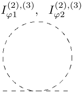
Figure 2: One-loop diagram from the scalar loops by the quartic interaction.

Next, we consider the corrections from the scalar quartic interactions (52). There are also four types of one-loop corrections to the scalar masses from the scalar loop contributions as in Figure 2, which are expressed as

Iφ​1(2)\displaystyle I^{(2)}_{\varphi 1} =8​i​g2Λ2​|N|​∑n=0∞∫d4​p(2​π)4​p2p2+α⁡(n+12),\displaystyle=\frac{8ig^{2}}{\Lambda^{2}}|N|\sum_{n=0}^{\infty}\int\frac{d^{4}p}{(2\pi)^{4}}\frac{p^{2}}{p^{2}+\alpha\left(n+\frac{1}{2}\right)}, (63)
Iφ​1(3)\displaystyle I^{(3)}_{\varphi 1} =8​i​g2Λ2​|N|​∑n=0∞∫d4​p(2​π)4​p2p2+α⁡(n+12),\displaystyle=\frac{8ig^{2}}{\Lambda^{2}}|N|\sum_{n=0}^{\infty}\int\frac{d^{4}p}{(2\pi)^{4}}\frac{p^{2}}{p^{2}+\alpha\left(n+\frac{1}{2}\right)}, (64)
Iφ​2(2)\displaystyle I^{(2)}_{\varphi 2} =16​i​g2Λ2​|N|​∑n=0∞∫d4​p(2​π)4​α​np2+α⁡(n+12),\displaystyle=\frac{16ig^{2}}{\Lambda^{2}}|N|\sum_{n=0}^{\infty}\int\frac{d^{4}p}{(2\pi)^{4}}\frac{\alpha n}{p^{2}+\alpha\left(n+\frac{1}{2}\right)}, (65)
Iφ​2(3)\displaystyle I^{(3)}_{\varphi 2} =16​i​g2Λ2​|N|​∑n=0∞∫d4​p(2​π)4​α⁡(n+1)p2+α⁡(n+12),\displaystyle=\frac{16ig^{2}}{\Lambda^{2}}|N|\sum_{n=0}^{\infty}\int\frac{d^{4}p}{(2\pi)^{4}}\frac{\alpha(n+1)}{p^{2}+\alpha\left(n+\frac{1}{2}\right)}, (66)

where the superscript (2), (3) means the contributions from φ~2,φ~3\widetilde{\varphi}^{2},\widetilde{\varphi}^{3} loops respectively. φ​1\varphi 1 and φ​2\varphi 2 represent corrections from the interactions in the first line and the second line of (52), respectively. Calculating these corrections similarly to the above gauge boson loop, we obtain

Iφ​1\displaystyle I_{\varphi 1} ≡Iφ​1(2)+Iφ​1(3)=−i​g2​α2​|N|π2​Λ2​(4​πα)ϵ​Γ​(ϵ−1)​ζ​[ϵ−2,1/2],\displaystyle\equiv I^{(2)}_{\varphi 1}+I^{(3)}_{\varphi 1}=-i\frac{g^{2}\alpha^{2}|N|}{\pi^{2}\Lambda^{2}}\left(\frac{4\pi}{\alpha}\right)^{\epsilon}\Gamma(\epsilon-1)\zeta[\epsilon-2,1/2], (67)
Iφ​2\displaystyle I_{\varphi 2} ≡Iφ​2(2)+Iφ​2(3)=+i​2​g2​α2​|N|π2​Λ2​(4​πα)ϵ​Γ​(ϵ−1)​ζ​[ϵ−2,1/2].\displaystyle\equiv I^{(2)}_{\varphi 2}+I^{(3)}_{\varphi 2}=+i\frac{2g^{2}\alpha^{2}|N|}{\pi^{2}\Lambda^{2}}\left(\frac{4\pi}{\alpha}\right)^{\epsilon}\Gamma(\epsilon-1)\zeta[\epsilon-2,1/2]. (68)

Summing up (67) and (68), we obtain the total scalar loop contributions to one-loop correction due to the scalar quartic interactions.

Iφ​φ​φ​φ≡Iφ​1+Iφ​2=+i​g2​α2​|N|π2​Λ2​(4​πα)ϵ​Γ​(ϵ−1)​ζ​[ϵ−2,1/2].\displaystyle I_{\varphi\varphi\varphi\varphi}\equiv I_{\varphi 1}+I_{\varphi 2}=+i\frac{g^{2}\alpha^{2}|N|}{\pi^{2}\Lambda^{2}}\left(\frac{4\pi}{\alpha}\right)^{\epsilon}\Gamma(\epsilon-1)\zeta[\epsilon-2,1/2]. (69)

4.2 One-loop Corrections from the Cubic Interactions

In the case of the corrections due to the cubic interactions, we note that one-loop corrections using both the cubic interaction in 𝒪⁡(Λ0)\mathcal{O}(\Lambda^{0}) and that in 𝒪⁡(1/Λ2)\mathcal{O}(1/\Lambda^{2}) appear. This is a nontrivial point in calculating the corrections in the presence of the higher dimensional operators.

Refer to caption
Figure 3: One-loop diagram from the gauge boson loops by the cubic interactions.

From the interacitons (33) and (53), there are four types of one-loop corrections to the scalar masses from the gauge boson loop contributions as in Figure 3 .

IA​3(2)\displaystyle I^{(2)}_{A3} =−32​i​g2Λ2|N|∑n=0∞∫d4​p(2​π)4​α⁡(n+1)​p2(p2+α​n)​(p2+α⁡(n+1)),\displaystyle=-\frac{32ig^{2}}{\Lambda^{2}}|N|\sum_{n=0}^{\infty}\int\frac{d^{4}p}{(2\pi)^{4}}\frac{\alpha(n+1)p^{2}}{(p^{2}+\alpha n)(p^{2}+\alpha(n+1))}, (70)
IA​3(3)\displaystyle I^{(3)}_{A3} =−32​i​g2Λ2|N|∑n=0∞∫d4​p(2​π)4​α⁡(n+1)​p2(p2+α⁡(n+1))​(p2+α⁡(n+2)),\displaystyle=-\frac{32ig^{2}}{\Lambda^{2}}|N|\sum_{n=0}^{\infty}\int\frac{d^{4}p}{(2\pi)^{4}}\frac{\alpha(n+1)p^{2}}{(p^{2}+\alpha(n+1))(p^{2}+\alpha(n+2))}, (71)
IA​4(2)\displaystyle I^{(2)}_{A4} =−32​i​g2Λ2|N|∑n=0∞∫d4​p(2​π)4​α⁡(n+1)​α​(n+12)(p2+α​n)​(p2+α⁡(n+1)),\displaystyle=-\frac{32ig^{2}}{\Lambda^{2}}|N|\sum_{n=0}^{\infty}\int\frac{d^{4}p}{(2\pi)^{4}}\frac{\alpha(n+1)\alpha\left(n+\frac{1}{2}\right)}{(p^{2}+\alpha n)(p^{2}+\alpha(n+1))}, (72)
IA​4(3)\displaystyle I^{(3)}_{A4} =−32​i​g2Λ2|N|∑n=0∞∫d4​p(2​π)4​α⁡(n+1)​α​(n+32)(p2+α⁡(n+1))​(p2+α⁡(n+2)).\displaystyle=-\frac{32ig^{2}}{\Lambda^{2}}|N|\sum_{n=0}^{\infty}\int\frac{d^{4}p}{(2\pi)^{4}}\frac{\alpha(n+1)\alpha\left(n+\frac{3}{2}\right)}{(p^{2}+\alpha(n+1))(p^{2}+\alpha(n+2))}. (73)

where A​3​(A​4)A3(A4) represents the contributions from the interactions of the first and the second (from the third to the sixth) lines in (53), respectively. Calculating these corrections by dimensional regularization, we find

IA​3\displaystyle I_{A3} ≡IA​3(2)+IA​3(3)=+i​4​g2​α2​|N|π2​Λ2​(4​πα)ϵ​Γ​(ϵ−1)​ζ​[ϵ−2,0],\displaystyle\equiv I^{(2)}_{A3}+I^{(3)}_{A3}=+i\frac{4g^{2}\alpha^{2}|N|}{\pi^{2}\Lambda^{2}}\left(\frac{4\pi}{\alpha}\right)^{\epsilon}\Gamma(\epsilon-1)\zeta[\epsilon-2,0], (74)
IA​4\displaystyle I_{A4} ≡IA​4(2)+IA​4(3)=−i​8​g2​α2​|N|π2​Λ2​(4​πα)ϵ​Γ​(ϵ−1)​ζ​[ϵ−2,0].\displaystyle\equiv I^{(2)}_{A4}+I^{(3)}_{A4}=-i\frac{8g^{2}\alpha^{2}|N|}{\pi^{2}\Lambda^{2}}\left(\frac{4\pi}{\alpha}\right)^{\epsilon}\Gamma(\epsilon-1)\zeta[\epsilon-2,0]. (75)

Summing up these results (74) and (75), we obtain the total one-loop corrections to the scalar masses from the gauge boson loop contributions.

Iφ​A​A≡IA​3+IA​4=−i​4​g2​α2​|N|π2​Λ2​(4​πα)ϵ​Γ​(ϵ−1)​ζ​[ϵ−2,0].\displaystyle I_{\varphi AA}\equiv I_{A3}+I_{A4}=-i\frac{4g^{2}\alpha^{2}|N|}{\pi^{2}\Lambda^{2}}\left(\frac{4\pi}{\alpha}\right)^{\epsilon}\Gamma(\epsilon-1)\zeta[\epsilon-2,0]. (76)
Refer to caption
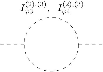
Figure 4: One-loop diagram from the scalar loops by the cubic interactions.

Next, we consider the corrections from (34) and (54), which also give four types of one-loop corrections from the scalar loop contributions as in Figure 4.

Iφ​3(2)\displaystyle I^{(2)}_{\varphi 3} =−8​i​g2Λ2|N|∑n=0∞∫d4​p(2​π)4​α⁡(n+1)​p2(p2+α⁡(n+12))​(p2+α⁡(n+32)),\displaystyle=-\frac{8ig^{2}}{\Lambda^{2}}|N|\sum_{n=0}^{\infty}\int\frac{d^{4}p}{(2\pi)^{4}}\frac{\alpha(n+1)p^{2}}{\left(p^{2}+\alpha\left(n+\frac{1}{2}\right)\right)\left(p^{2}+\alpha\left(n+\frac{3}{2}\right)\right)}, (77)
Iφ​3(3)\displaystyle I^{(3)}_{\varphi 3} =−8​i​g2Λ2|N|∑n=0∞∫d4​p(2​π)4​α⁡(n+1)​p2(p2+α⁡(n+12))​(p2+α⁡(n+32)),\displaystyle=-\frac{8ig^{2}}{\Lambda^{2}}|N|\sum_{n=0}^{\infty}\int\frac{d^{4}p}{(2\pi)^{4}}\frac{\alpha(n+1)p^{2}}{\left(p^{2}+\alpha\left(n+\frac{1}{2}\right)\right)\left(p^{2}+\alpha\left(n+\frac{3}{2}\right)\right)}, (78)
Iφ​4(2)\displaystyle I^{(2)}_{\varphi 4} =−8​i​g2Λ2|N|∑n=0∞∫d4​p(2​π)4​α⁡(n+1)​α​(n−14)(p2+α⁡(n+12))​(p2+α⁡(n+32)),\displaystyle=-\frac{8ig^{2}}{\Lambda^{2}}|N|\sum_{n=0}^{\infty}\int\frac{d^{4}p}{(2\pi)^{4}}\frac{\alpha(n+1)\alpha\left(n-\frac{1}{4}\right)}{\left(p^{2}+\alpha\left(n+\frac{1}{2}\right)\right)\left(p^{2}+\alpha\left(n+\frac{3}{2}\right)\right)}, (79)
Iφ​4(3)\displaystyle I^{(3)}_{\varphi 4} =−8​i​g2Λ2|N|∑n=0∞∫d4​p(2​π)4​α⁡(n+1)​α​(n+94)(p2+α⁡(n+12))​(p2+α⁡(n+32)).\displaystyle=-\frac{8ig^{2}}{\Lambda^{2}}|N|\sum_{n=0}^{\infty}\int\frac{d^{4}p}{(2\pi)^{4}}\frac{\alpha(n+1)\alpha\left(n+\frac{9}{4}\right)}{\left(p^{2}+\alpha\left(n+\frac{1}{2}\right)\right)\left(p^{2}+\alpha\left(n+\frac{3}{2}\right)\right)}. (80)

φ​3​(φ​4)\varphi 3(\varphi 4) represents the contributions from the interactions of the first and the second (from the third to the sixth) lines in (54), respectively. By similar calculations, we find

Iφ​3\displaystyle I_{\varphi 3} ≡Iφ​3(2)+Iφ​3(3)=+i​g2​α2​|N|π2​Λ2​(4​πϵ)ϵ​Γ​(ϵ−1)​ζ​[ϵ−2,1/2],\displaystyle\equiv I^{(2)}_{\varphi 3}+I^{(3)}_{\varphi 3}=+i\frac{g^{2}\alpha^{2}|N|}{\pi^{2}\Lambda^{2}}\left(\frac{4\pi}{\epsilon}\right)^{\epsilon}\Gamma(\epsilon-1)\zeta[\epsilon-2,1/2], (81)
Iφ​4\displaystyle I_{\varphi 4} ≡Iφ​4(2)+Iφ​4(3)=−i​2​g2​α2​|N|π2​Λ2​(4​πα)ϵ​Γ​(ϵ−1)​ζ​[ϵ−2,1/2].\displaystyle\equiv I^{(2)}_{\varphi 4}+I^{(3)}_{\varphi 4}=-i\frac{2g^{2}\alpha^{2}|N|}{\pi^{2}\Lambda^{2}}\left(\frac{4\pi}{\alpha}\right)^{\epsilon}\Gamma(\epsilon-1)\zeta[\epsilon-2,1/2]. (82)

Summing up (81) and (82), we obtain the total one-loop corrections to the scalar masses from the scalar loop contributions.

Iφ​φ​φ\displaystyle I_{\varphi\varphi\varphi} ≡Iφ​3+Iφ​4=−i​g2​α2​|N|π2​Λ2​(4​πα)ϵ​Γ​(ϵ−1)​ζ​[ϵ−2,1/2].\displaystyle\equiv I_{\varphi 3}+I_{\varphi 4}=-i\frac{g^{2}\alpha^{2}|N|}{\pi^{2}\Lambda^{2}}\left(\frac{4\pi}{\alpha}\right)^{\epsilon}\Gamma(\epsilon-1)\zeta[\epsilon-2,1/2]. (83)

4.3 Cancellation of One-loop Corrections to Scalar Mass at 𝒪⁡(1/Λ2)\mathcal{O}(1/\Lambda^{2})

Summing up all of the results (62), (69), (76) and (83), we can verify that one-loop corrections to the scalar masses are indeed cancelled at the leading order of 1/Λ21/\Lambda^{2}.

Iφ​φ​A​A+Iφ​A​A=0,\displaystyle I_{\varphi\varphi AA}+I_{\varphi AA}=0, (84)
Iφ​φ​φ​φ+Iφ​φ​φ=0.\displaystyle I_{\varphi\varphi\varphi\varphi}+I_{\varphi\varphi\varphi}=0. (85)

As can be seen, the gauge loop contributions and the scalar loop contributions are independently cancelled. In particular, the scalar loop contributions can be cancelled without the ghost loop contributions, which is different from the case of Yang-Mills theory [10].

4.4 Comments on the Corrections from the Higher Dimensional Operators More Than 𝒪⁡(1/Λ4)\mathcal{O}(1/\Lambda^{4})

Finally, we would like to comment on the generalization of our discussion, namely, the corrections from the higher dimensional operators more than 𝒪⁡(1/Λ4)\mathcal{O}(1/\Lambda^{4}). In this case, the cancellation of the one-loop corrections to the scalar masses becomes more involved. For instance, let us consider the next to leading order higher dimensional operators (39). We immediately find that the first term vanishes because of the traceless condition for SU(2) generators as in the section 3.1 and the third term also vanishes because of the properties of totally anti-symmetric tensor and the trace of generators as in the section 3.2. Thus, 𝒪2​(D,F)\mathcal{O}_{2}(D,F) is reduced to

𝒪2​(D,F)\displaystyle\mathcal{O}_{2}(D,F) =Tr⁡[Dk​DL​FM​N​DK​DL​FM​N]+Tr⁡[FM​N​FM​N​FA​B​FA​B].\displaystyle=\mathrm{Tr}[D_{k}D_{L}F_{MN}D^{K}D^{L}F^{MN}]+\mathrm{Tr}[F_{MN}F^{MN}F_{AB}F^{AB}]. (86)

If we use two kinds of cubic interactions (53) and (54), we obtain some one-loop corrections at the second order of 1/Λ21/\Lambda^{2}, however these corrections are not cancelled because we must take into account the contributions with the operators of 𝒪⁡(1/Λ0)\mathcal{O}(1/\Lambda^{0}) and 𝒪⁡(1/Λ4)\mathcal{O}(1/\Lambda^{4}). Even at 𝒪⁡(1/Λ4)\mathcal{O}(1/\Lambda^{4}), although it is relatively easy to calculate the second term in (86), the first term in (86) is found to have huge number of interaction terms which are relevant to the one-loop corrections to the scalar masses. At higher order than 𝒪⁡(1/Λ4)\mathcal{O}(1/\Lambda^{4}), we need to consider carefully the variety of combinations among the operators different order of 1/Λ21/\Lambda^{2} and it becomes more complicated. Such an analysis is very interesting, however it is beyond the scope of this paper and we leave it for a future study.

5 Summary

Since the higher dimensional theory is nonrenormalizable, the higher dimensional operators consistent with symmetry of the theory should be taken into account in the Lagrangian. In this paper, we have shown that one-loop corrections to the masses of the scalar fields, which are zero modes of extra components of the higher dimensional gauge fields, are indeed cancelled in flux compactification of a six dimensional SU(2) Yang-Mills theory including the leading order of higher dimensional operators. Even if the higher dimensional operators are taken into account, the cancellation is expected to be true as long as the zero mode of the scalar fields are NG bosons with respect to the translational symmetry in compactified space. The statement is straightforward, but the cancellation itself is not so trivial since the contributions to the scalar masses come from the interactions in the different order of the higher dimensional operators. In fact, the one-loop corrections to the scalar masses at 𝒪⁡(1/Λ2){\cal O}(1/\Lambda^{2}) are generated from the cubic interactions of higher dimensional operators at 𝒪⁡(1/Λ0){\cal O}(1/\Lambda^{0}) and 𝒪⁡(1/Λ2){\cal O}(1/\Lambda^{2}) and were shown to be cancelled in this paper. This cancellation would not be changed even if we take into account the fermion contributions.

One of the interesting applications of our results obtained in this paper is to identify the scalar field with the SM Higgs field. Since the information on the new physics are encoded in the higher dimensional operators consistent with the SM gauge symmetry, our observations and results in this paper are quite useful. As mentioned in the introduction, since the Higgs field is massless as it stands, the translational symmetry in compactified space must be explicitly broken at weak scale to give a mass to the Higgs field. Understanding a mechanism to realize this situation is a next issue in our future study.

Acknowledgments

This work is supported in part by JSPS KAKENHI Grant Number JP17K05420 (N.M.).

Appendix A Detail calculations for one-loop corrections to the scalar masses

In this Appendix, the calculations in the main text are explained in detail [8, 13].

A.1 Loop Integral Fomula and Hurwitz Zeta Function

In the calculation of the loop integral, we employ the dimensional regularization and use these integrals in Euclidean space.

∫dd​p(2​π)d​1(p2+Δ)n\displaystyle\int\frac{d^{d}p}{(2\pi)^{d}}\frac{1}{\left(p^{2}+\Delta\right)^{n}} =1(4​π)d/2​Γ⁡(n−d2)Γ⁡(n)​(1Δ)n−d2,\displaystyle=\frac{1}{(4\pi)^{d/2}}\frac{\Gamma\left(n-\frac{d}{2}\right)}{\Gamma(n)}\left(\frac{1}{\Delta}\right)^{n-\frac{d}{2}}, (87)
∫dd​p(2​π)d​pμ​pν(p2+Δ)n\displaystyle\int\frac{d^{d}p}{(2\pi)^{d}}\frac{p_{\mu}p_{\nu}}{\left(p^{2}+\Delta\right)^{n}} =1(4​π)d/2​δμ​ν2​Γ⁡(n−d2−1)Γ⁡(n)​(1Δ)n−d2−1,\displaystyle=\frac{1}{(4\pi)^{d/2}}\frac{\delta_{\mu\nu}}{2}\frac{\Gamma\left(n-\frac{d}{2}-1\right)}{\Gamma(n)}\left(\frac{1}{\Delta}\right)^{n-\frac{d}{2}-1}, (88)

where d=4−2​ϵd=4-2\epsilon and Γ⁡(n)\Gamma(n) is gamma function.

As for the mode summation with respect to nn, it is convenient to use Hurwitz zeta function

ζ⁡[s,a]=∑n=0∞1(n+a)s.\displaystyle\zeta[s,a]=\sum_{n=0}^{\infty}\frac{1}{(n+a)^{s}}. (89)

In the main text, we deal with ζ⁡[ϵ−2,a]\zeta[\epsilon-2,a] and ζ⁡[ϵ−3,a]\zeta[\epsilon-3,a] (a=0,1/2,1,3/2,2)(a=0,1/2,1,3/2,2), therefore, we summarize these values.

ζ⁡[ϵ−2,0]\displaystyle\zeta[\epsilon-2,0] =ζ⁡(3)4​π2​ϵ,\displaystyle=\frac{\zeta(3)}{4\pi^{2}}\epsilon, ζ⁡[ϵ−3,0]\displaystyle\zeta[\epsilon-3,0] =1120+ζ′​(−3)​ϵ\displaystyle=\frac{1}{120}+\zeta^{\prime}(-3)\epsilon
ζ⁡[ϵ−2,1/2]\displaystyle\zeta[\epsilon-2,1/2] =3​ζ​(3)16​π2​ϵ,\displaystyle=\frac{3\zeta(3)}{16\pi^{2}}\epsilon, ζ⁡[ϵ−3,1/2]\displaystyle\zeta[\epsilon-3,1/2] =−7960+(ln⁡2960−78​ζ′​(−3))​ϵ\displaystyle=-\frac{7}{960}+\left(\frac{\ln 2}{960}-\frac{7}{8}\zeta^{\prime}(-3)\right)\epsilon
ζ⁡[ϵ−2,1]\displaystyle\zeta[\epsilon-2,1] =ζ⁡(3)4​π2​ϵ,\displaystyle=\frac{\zeta(3)}{4\pi^{2}}\epsilon, ζ⁡[ϵ−3,1]\displaystyle\zeta[\epsilon-3,1] =1120+ζ′​(−3)​ϵ\displaystyle=\frac{1}{120}+\zeta^{\prime}(-3)\epsilon
ζ⁡[ϵ−2,3/2]\displaystyle\zeta[\epsilon-2,3/2] =−14+(−ln⁡24+3​ζ​(3)16​π2)​ϵ,\displaystyle=-\frac{1}{4}+\left(-\frac{\ln 2}{4}+\frac{3\zeta(3)}{16\pi^{2}}\right)\epsilon, ζ⁡[ϵ−3,3/2]\displaystyle\zeta[\epsilon-3,3/2] =−127960+(−119​ln⁡2960−78​ζ′​(−3))​ϵ\displaystyle=-\frac{127}{960}+\left(-\frac{119\ln 2}{960}-\frac{7}{8}\zeta^{\prime}(-3)\right)\epsilon
ζ⁡[ϵ−2,2]\displaystyle\zeta[\epsilon-2,2] =−1+ζ⁡(3)4​π2​ϵ,\displaystyle=-1+\frac{\zeta(3)}{4\pi^{2}}\epsilon, ζ⁡[ϵ−3,2]\displaystyle\zeta[\epsilon-3,2] =−119120+ζ′​(−3)​ϵ\displaystyle=-\frac{119}{120}+\zeta^{\prime}(-3)\epsilon

A.2 Case (56) and (57)

To calculate (56), JJ is defined as

J≡∑n=0∞∫d4​p(2​π)4​p2p2+α​n.\displaystyle J\equiv\sum_{n=0}^{\infty}\int\frac{d^{4}p}{(2\pi)^{4}}\frac{p^{2}}{p^{2}+\alpha n}. (90)

Using (88), JJ can be expressed as

J\displaystyle J =∑n=0∞1(4​π)d/2​d2​Γ​(−d2)​(1α​n)−d2\displaystyle=\sum_{n=0}^{\infty}\frac{1}{(4\pi)^{d/2}}\frac{d}{2}\Gamma\left(-\frac{d}{2}\right)\left(\frac{1}{\alpha n}\right)^{-\frac{d}{2}}
=−α216​π2​(4​πα)ϵ​Γ​(ϵ−1)​ζ​[ϵ−2,0].\displaystyle=-\frac{\alpha^{2}}{16\pi^{2}}\left(\frac{4\pi}{\alpha}\right)^{\epsilon}\Gamma(\epsilon-1)\zeta[\epsilon-2,0]. (91)

Similarly, to calculate (57), J′J^{\prime} is defined as and using (88), we find

J′\displaystyle J^{\prime} ≡∑n=0∞∫d4​p(2​π)4​p2p2+α⁡(n+1)\displaystyle\equiv\sum_{n=0}^{\infty}\int\frac{d^{4}p}{(2\pi)^{4}}\frac{p^{2}}{p^{2}+\alpha(n+1)}
=−α216​π2​(4​πα)ϵ​Γ​(ϵ−1)​ζ​[ϵ−2,1].\displaystyle=-\frac{\alpha^{2}}{16\pi^{2}}\left(\frac{4\pi}{\alpha}\right)^{\epsilon}\Gamma(\epsilon-1)\zeta[\epsilon-2,1]. (92)

Noting the fact that ζ⁡[ϵ−2,1]=ζ⁡[ϵ−2,0]\zeta[\epsilon-2,1]=\zeta[\epsilon-2,0], JJ and J′J^{\prime} are found to be same. Thus, IA​1I_{A1} is computed as

IA​1\displaystyle I_{A1} ≡IA​1(2)+IA​1(3)=64​i​g2Λ2​|N|​J\displaystyle\equiv I^{(2)}_{A1}+I^{(3)}_{A1}=\frac{64ig^{2}}{\Lambda^{2}}|N|J
=−i​4​g2​α2​|N|π2​Λ2​(4​πα)ϵ​Γ​(ϵ−1)​ζ​[ϵ−2,0].\displaystyle=-i\frac{4g^{2}\alpha^{2}|N|}{\pi^{2}\Lambda^{2}}\left(\frac{4\pi}{\alpha}\right)^{\epsilon}\Gamma(\epsilon-1)\zeta[\epsilon-2,0]. (93)

A.3 Case (58) and (59)

To calculate (58), KK is defined as

K≡∑n=0∞α​n​∫d4​p(2​π)4​1p2+α​n.\displaystyle K\equiv\sum_{n=0}^{\infty}\alpha n\int\frac{d^{4}p}{(2\pi)^{4}}\frac{1}{p^{2}+\alpha n}. (94)

Using (87), KK can be expressed as

K\displaystyle K =∑n=0∞α​n​1(4​π)d/2​Γ​(1−d2)​(1α​n)1−d/2\displaystyle=\sum_{n=0}^{\infty}\alpha n\frac{1}{(4\pi)^{d/2}}\Gamma\left(1-\frac{d}{2}\right)\left(\frac{1}{\alpha n}\right)^{1-d/2}
=α2(4​π)2​(4​πα)ϵ​Γ​(ϵ−1)​ζ​[ϵ−2,0].\displaystyle=\frac{\alpha^{2}}{(4\pi)^{2}}\left(\frac{4\pi}{\alpha}\right)^{\epsilon}\Gamma(\epsilon-1)\zeta[\epsilon-2,0]. (95)

Similarly, to calculate (59), K′K^{\prime} is defined as and using (87), we find

K′\displaystyle K^{\prime} ≡∑n=0∞α⁡(n+1)​∫d4​p(2​π)4​1p2+α⁡(n+1)\displaystyle\equiv\sum_{n=0}^{\infty}\alpha(n+1)\int\frac{d^{4}p}{(2\pi)^{4}}\frac{1}{p^{2}+\alpha(n+1)}
=α2(4​π)2​(4​πα)ϵ​Γ​(ϵ−1)​ζ​[ϵ−2,1].\displaystyle=\frac{\alpha^{2}}{(4\pi)^{2}}\left(\frac{4\pi}{\alpha}\right)^{\epsilon}\Gamma(\epsilon-1)\zeta[\epsilon-2,1]. (96)

Because of ζ⁡[ϵ−2,1]=ζ⁡[ϵ−2,0]\zeta[\epsilon-2,1]=\zeta[\epsilon-2,0] again, KK and K′K^{\prime} are found to be same. Thus, IA​2I_{A2} is computed as

IA​2\displaystyle I_{A2} ≡IA​2(2)+IA​2(3)=128​i​g2Λ2​|N|​K\displaystyle\equiv I^{(2)}_{A2}+I^{(3)}_{A2}=\frac{128ig^{2}}{\Lambda^{2}}|N|K
=+i​8​g2​α2​|N|π2​Λ2​(4​πα)ϵ​Γ​(ϵ−1)​ζ​[ϵ−2,0].\displaystyle=+i\frac{8g^{2}\alpha^{2}|N|}{\pi^{2}\Lambda^{2}}\left(\frac{4\pi}{\alpha}\right)^{\epsilon}\Gamma(\epsilon-1)\zeta[\epsilon-2,0]. (97)

A.4 Case (63) and (64)

To calculate (63) and (64), LL is defined as

L≡∑n=0∞∫d4​p(2​π)4​p2p2+α⁡(n+12).\displaystyle L\equiv\sum_{n=0}^{\infty}\int\frac{d^{4}p}{(2\pi)^{4}}\frac{p^{2}}{p^{2}+\alpha\left(n+\frac{1}{2}\right)}. (98)

Using (88), LL is expressed to be

L\displaystyle L =∑n=0∞1(4​π)d/2​d2​Γ​(−d2)​(1α⁡(n+12))−d2\displaystyle=\sum_{n=0}^{\infty}\frac{1}{(4\pi)^{d/2}}\frac{d}{2}\Gamma\left(-\frac{d}{2}\right)\left(\frac{1}{\alpha\left(n+\frac{1}{2}\right)}\right)^{-\frac{d}{2}}
=−α216​π2​(4​πα)ϵ​Γ​(ϵ−1)​ζ​[ϵ−2,1/2].\displaystyle=-\frac{\alpha^{2}}{16\pi^{2}}\left(\frac{4\pi}{\alpha}\right)^{\epsilon}\Gamma(\epsilon-1)\zeta[\epsilon-2,1/2]. (99)

Thus, Iφ​1I_{\varphi 1} is computed as

Iφ​1\displaystyle I_{\varphi 1} ≡Iφ​1(2)+Iφ​1(3)=16​i​g2Λ2​|N|​L\displaystyle\equiv I^{(2)}_{\varphi 1}+I^{(3)}_{\varphi 1}=\frac{16ig^{2}}{\Lambda^{2}}|N|L
=−i​g2​α2​|N|π2​Λ2​(4​πα)ϵ​Γ​(ϵ−1)​ζ​[ϵ−2,1/2].\displaystyle=-i\frac{g^{2}\alpha^{2}|N|}{\pi^{2}\Lambda^{2}}\left(\frac{4\pi}{\alpha}\right)^{\epsilon}\Gamma(\epsilon-1)\zeta[\epsilon-2,1/2]. (100)

A.5 Case (65) and (66)

In this calculation, it is easy to calculate Iφ​2I_{\varphi 2} defined as Iφ​2≡Iφ​2(2)+Iφ​2(3)I_{\varphi 2}\equiv I^{(2)}_{\varphi 2}+I^{(3)}_{\varphi 2} rather than computations of Iφ​2(2)I^{(2)}_{\varphi 2} and Iφ​2(3)I^{(3)}_{\varphi 2} individually. Then, Iφ​2I_{\varphi 2} is given by

Iφ​2\displaystyle I_{\varphi 2} =Iφ​2(2)+Iφ​2(3)\displaystyle=I^{(2)}_{\varphi 2}+I^{(3)}_{\varphi 2}
=32​i​g2Λ2​|N|​∑n=0∞∫d4​p(2​π)4​α⁡(n+12)p2+α⁡(n+12).\displaystyle=\frac{32ig^{2}}{\Lambda^{2}}|N|\sum_{n=0}^{\infty}\int\frac{d^{4}p}{(2\pi)^{4}}\frac{\alpha\left(n+\frac{1}{2}\right)}{p^{2}+\alpha\left(n+\frac{1}{2}\right)}. (101)

To calculate Iφ​2I_{\varphi 2}, MM is defined as

M≡∑n=0∞∫d4​p(2​π)4​α⁡(n+12)p2+α⁡(n+12).\displaystyle M\equiv\sum_{n=0}^{\infty}\int\frac{d^{4}p}{(2\pi)^{4}}\frac{\alpha\left(n+\frac{1}{2}\right)}{p^{2}+\alpha\left(n+\frac{1}{2}\right)}. (102)

Using (87), MM expresses

M=α216​π2​(4​πα)ϵ​Γ​(ϵ−1)​ζ​[ϵ−2,1/2]\displaystyle M=\frac{\alpha^{2}}{16\pi^{2}}\left(\frac{4\pi}{\alpha}\right)^{\epsilon}\Gamma(\epsilon-1)\zeta[\epsilon-2,1/2] (103)

Thus, Iφ​2I_{\varphi 2} is computed as

Iφ​2\displaystyle I_{\varphi 2} =32​i​g2Λ2​|N|​M\displaystyle=\frac{32ig^{2}}{\Lambda^{2}}|N|M
=+i​2​g2​α2​|N|π2​Λ2​(4​πα)ϵ​Γ​(ϵ−1)​ζ​[ϵ−2,1/2].\displaystyle=+i\frac{2g^{2}\alpha^{2}|N|}{\pi^{2}\Lambda^{2}}\left(\frac{4\pi}{\alpha}\right)^{\epsilon}\Gamma(\epsilon-1)\zeta[\epsilon-2,1/2]. (104)

A.6 Case (70) and (71)

To calculate (70), AA is defined as

A\displaystyle A ≡∑n=0∞∫d4​p(2​π)4​α⁡(n+1)​p2(p2+α​n)​(p2+α⁡(n+1))\displaystyle\equiv\sum_{n=0}^{\infty}\int\frac{d^{4}p}{(2\pi)^{4}}\frac{\alpha(n+1)p^{2}}{(p^{2}+\alpha n)(p^{2}+\alpha(n+1))}
=∑n=0∞α⁡(n+1)​∫01d​x​∫d4​p(2​π)4​p2(p2+Δ⁡(x,n))2,\displaystyle=\sum_{n=0}^{\infty}\alpha(n+1)\int_{0}^{1}dx\int\frac{d^{4}p}{(2\pi)^{4}}\frac{p^{2}}{(p^{2}+\Delta(x,n))^{2}}, (105)

where Δ⁡(x,n)=α⁡(n+1)−α​x\Delta(x,n)=\alpha(n+1)-\alpha x. Using (88), AA is expressed as

A\displaystyle A =∑n=0∞α⁡(n+1)​1(4​π)d/2​d2​Γ​(1−d2)​(1Δ)1−d2\displaystyle=\sum_{n=0}^{\infty}\alpha(n+1)\frac{1}{(4\pi)^{d/2}}\frac{d}{2}\Gamma\left(1-\frac{d}{2}\right)\left(\frac{1}{\Delta}\right)^{1-\frac{d}{2}}
=(−1)ϵ−1​α216​π2​(4​πα)ϵ​(2−ϵ)​Γ​(ϵ−1)​∑n=0∞(n+1)​∫01d​x​(1x−α⁡(n+1))ϵ−1.\displaystyle=(-1)^{\epsilon-1}\frac{\alpha^{2}}{16\pi^{2}}\left(\frac{4\pi}{\alpha}\right)^{\epsilon}(2-\epsilon)\Gamma(\epsilon-1)\sum_{n=0}^{\infty}(n+1)\int_{0}^{1}dx\left(\frac{1}{x-\alpha(n+1)}\right)^{\epsilon-1}. (106)

Performing the integral over xx, we find

A\displaystyle A =−α216​π2(4​πα)ϵΓ(ϵ−1)∑n=0∞(n+1)(1nϵ−2−1(n+1)ϵ−2)\displaystyle=-\frac{\alpha^{2}}{16\pi^{2}}\left(\frac{4\pi}{\alpha}\right)^{\epsilon}\Gamma(\epsilon-1)\sum_{n=0}^{\infty}(n+1)\left(\frac{1}{n^{\epsilon-2}}-\frac{1}{(n+1)^{\epsilon-2}}\right)
=−α216​π2​(4​πα)ϵ​Γ​(ϵ−1)​(ζ⁡[ϵ−3,0]+ζ⁡[ϵ−2,0]−ζ⁡[ϵ−3,1])\displaystyle=-\frac{\alpha^{2}}{16\pi^{2}}\left(\frac{4\pi}{\alpha}\right)^{\epsilon}\Gamma(\epsilon-1)\Big(\zeta[\epsilon-3,0]+\zeta[\epsilon-2,0]-\zeta[\epsilon-3,1]\Big)
=−α216​π2​(4​πα)ϵ​Γ​(ϵ−1)​ζ​[ϵ−2,0].\displaystyle=-\frac{\alpha^{2}}{16\pi^{2}}\left(\frac{4\pi}{\alpha}\right)^{\epsilon}\Gamma(\epsilon-1)\zeta[\epsilon-2,0]. (107)

Similarly, to calculate (71), A′A^{\prime} is defined as

A′\displaystyle A^{\prime} ≡∑n=0∞∫d4​p(2​π)4​α⁡(n+1)​p2(p2+α⁡(n+1))​(p2+α⁡(n+2))\displaystyle\equiv\sum_{n=0}^{\infty}\int\frac{d^{4}p}{(2\pi)^{4}}\frac{\alpha(n+1)p^{2}}{(p^{2}+\alpha(n+1))(p^{2}+\alpha(n+2))}
=∑n=0∞α⁡(n+1)​∫01d​x​∫d4​p(2​π)4​p2(p2+Δ′​(x,n))2,\displaystyle=\sum_{n=0}^{\infty}\alpha(n+1)\int_{0}^{1}dx\int\frac{d^{4}p}{(2\pi)^{4}}\frac{p^{2}}{(p^{2}+\Delta^{\prime}(x,n))^{2}}, (108)

where Δ′​(x,n)=α⁡(n+2)−α​x\Delta^{\prime}(x,n)=\alpha(n+2)-\alpha x. Using (88) and performing the integral over xx, we find

A′\displaystyle A^{\prime} =−α216​π2(4​πα)ϵΓ(ϵ−1)∑n=0∞(n+1)(1(n+1)ϵ−2−1(n+2)ϵ−2)\displaystyle=-\frac{\alpha^{2}}{16\pi^{2}}\left(\frac{4\pi}{\alpha}\right)^{\epsilon}\Gamma(\epsilon-1)\sum_{n=0}^{\infty}(n+1)\left(\frac{1}{(n+1)^{\epsilon-2}}-\frac{1}{(n+2)^{\epsilon-2}}\right)
=−α216​π2​(4​πα)ϵ​Γ​(ϵ−1)​(ζ⁡[ϵ−3,1]−ζ⁡[ϵ−3,2]+ζ⁡[ϵ−2,2])\displaystyle=-\frac{\alpha^{2}}{16\pi^{2}}\left(\frac{4\pi}{\alpha}\right)^{\epsilon}\Gamma(\epsilon-1)\Big(\zeta[\epsilon-3,1]-\zeta[\epsilon-3,2]+\zeta[\epsilon-2,2]\Big)
=−α216​π2​(4​πα)ϵ​Γ​(ϵ−1)​ζ​[ϵ−2,0].\displaystyle=-\frac{\alpha^{2}}{16\pi^{2}}\left(\frac{4\pi}{\alpha}\right)^{\epsilon}\Gamma(\epsilon-1)\zeta[\epsilon-2,0]. (109)

Thus, IA​3I_{A3} is computed as

IA​3\displaystyle I_{A3} ≡IA​3(2)+IA​3(3)=−32​i​g2Λ2​|N|​(A+A′)\displaystyle\equiv I^{(2)}_{A3}+I^{(3)}_{A3}=-\frac{32ig^{2}}{\Lambda^{2}}|N|(A+A^{\prime})
=+i​4​g2​α2​|N|π2​Λ2​(4​πα)ϵ​Γ​(ϵ−1)​ζ​[ϵ−2,0].\displaystyle=+i\frac{4g^{2}\alpha^{2}|N|}{\pi^{2}\Lambda^{2}}\left(\frac{4\pi}{\alpha}\right)^{\epsilon}\Gamma(\epsilon-1)\zeta[\epsilon-2,0]. (110)

A.7 Case (72) and (73)

To calculate (72), BB is defined as

B\displaystyle B ≡∑n=0∞∫d4​p(2​π)4​α⁡(n+1)​α​(n+12)(p2+α​n)​(p2+α⁡(n+1))\displaystyle\equiv\sum_{n=0}^{\infty}\int\frac{d^{4}p}{(2\pi)^{4}}\frac{\alpha(n+1)\alpha\left(n+\frac{1}{2}\right)}{(p^{2}+\alpha n)(p^{2}+\alpha(n+1))}
=α2​∑n=0∞(n+1)​(n+12)​∫01d​x​∫d4​p(2​π)4​1(p2+Δ⁡(x,n))2,\displaystyle=\alpha^{2}\sum_{n=0}^{\infty}(n+1)\left(n+\frac{1}{2}\right)\int_{0}^{1}dx\int\frac{d^{4}p}{(2\pi)^{4}}\frac{1}{(p^{2}+\Delta(x,n))^{2}}, (111)

where Δ⁡(x,n)=α⁡(n+1)−α​x\Delta(x,n)=\alpha(n+1)-\alpha x. Using (87), BB is expressed as

B\displaystyle B =α2​∑n=0∞(n+1)​(n+12)​∫01d​x​1(4​π)d/2​Γ​(2−d2)​(1Δ)2−d2\displaystyle=\alpha^{2}\sum_{n=0}^{\infty}(n+1)\left(n+\frac{1}{2}\right)\int_{0}^{1}dx\frac{1}{(4\pi)^{d/2}}\Gamma\left(2-\frac{d}{2}\right)\left(\frac{1}{\Delta}\right)^{2-\frac{d}{2}}
=(−1)ϵ​α216​π2​(4​πα)ϵ​Γ​(ϵ)​∑n=0∞(n+1)​(n+12)​∫01d​x​(1x−(n+1))ϵ.\displaystyle=(-1)^{\epsilon}\frac{\alpha^{2}}{16\pi^{2}}\left(\frac{4\pi}{\alpha}\right)^{\epsilon}\Gamma(\epsilon)\sum_{n=0}^{\infty}(n+1)\left(n+\frac{1}{2}\right)\int_{0}^{1}dx\left(\frac{1}{x-(n+1)}\right)^{\epsilon}. (112)

Performing the integral over xx, we find

B\displaystyle B =−α216​π2(4​πα)ϵΓ(ϵ−1)∑n=0∞(n+1)(n+12)(−1nϵ−1+1(n+1)ϵ−1).\displaystyle=-\frac{\alpha^{2}}{16\pi^{2}}\left(\frac{4\pi}{\alpha}\right)^{\epsilon}\Gamma(\epsilon-1)\sum_{n=0}^{\infty}(n+1)\left(n+\frac{1}{2}\right)\left(-\frac{1}{n^{\epsilon-1}}+\frac{1}{(n+1)^{\epsilon-1}}\right). (113)

We compute the part of mode summation as follows.

(S​u​m)\displaystyle(Sum) =∑n=0∞(n+1)​(n+12)​(−1nϵ−1+1(n+1)ϵ−1)\displaystyle=\sum_{n=0}^{\infty}(n+1)\left(n+\frac{1}{2}\right)\left(-\frac{1}{n^{\epsilon-1}}+\frac{1}{(n+1)^{\epsilon-1}}\right)
=∑n=0∞(−1nϵ−3−12​1nϵ−2−1nϵ−2−12​1nϵ−1+1(n+1)ϵ−3−12​1(n+1)ϵ−2)\displaystyle=\sum_{n=0}^{\infty}\left(-\frac{1}{n^{\epsilon-3}}-\frac{1}{2}\frac{1}{n^{\epsilon-2}}-\frac{1}{n^{\epsilon-2}}-\frac{1}{2}\frac{1}{n^{\epsilon-1}}+\frac{1}{(n+1)^{\epsilon-3}}-\frac{1}{2}\frac{1}{(n+1)^{\epsilon-2}}\right)
=−2​ζ​[ϵ−2,0]−12​ζ​[ϵ−1,0],\displaystyle=-2\zeta[\epsilon-2,0]-\frac{1}{2}\zeta[\epsilon-1,0],

where we use the Hurwitz zeta functions in A.1. Thus, BB is computed as

B\displaystyle B =α216​π2​(4​πα)ϵ​Γ​(ϵ−1)​(2​ζ​[ϵ−2,0]+12​ζ​[ϵ−1,0]).\displaystyle=\frac{\alpha^{2}}{16\pi^{2}}\left(\frac{4\pi}{\alpha}\right)^{\epsilon}\Gamma(\epsilon-1)\left(2\zeta[\epsilon-2,0]+\frac{1}{2}\zeta[\epsilon-1,0]\right). (114)

Similarly, to calculate (73), B′B^{\prime} is defined as

B′\displaystyle B^{\prime} ≡∑n=0∞∫d4​p(2​π)4​α⁡(n+1)​α​(n+32)(p2+α⁡(n+1))​(p2+α⁡(n+2))\displaystyle\equiv\sum_{n=0}^{\infty}\int\frac{d^{4}p}{(2\pi)^{4}}\frac{\alpha(n+1)\alpha\left(n+\frac{3}{2}\right)}{(p^{2}+\alpha(n+1))(p^{2}+\alpha(n+2))}
=α2​∑n=0∞(n+1)​(n+32)​∫01d​x​∫d4​p(2​π)4​1(p2+Δ′​(x,n))2,\displaystyle=\alpha^{2}\sum_{n=0}^{\infty}(n+1)\left(n+\frac{3}{2}\right)\int_{0}^{1}dx\int\frac{d^{4}p}{(2\pi)^{4}}\frac{1}{(p^{2}+\Delta^{\prime}(x,n))^{2}}, (115)

where Δ′​(x,n)=α⁡(n+2)−α​x\Delta^{\prime}(x,n)=\alpha(n+2)-\alpha x. Using (87) and performing the integral over xx,

B′\displaystyle B^{\prime} =−α216​π2(4​πα)ϵΓ(ϵ−1)∑n=0∞(n+1)(n+32)(−1(n+1)ϵ−1+1(n+2)ϵ−1).\displaystyle=-\frac{\alpha^{2}}{16\pi^{2}}\left(\frac{4\pi}{\alpha}\right)^{\epsilon}\Gamma(\epsilon-1)\sum_{n=0}^{\infty}(n+1)\left(n+\frac{3}{2}\right)\left(-\frac{1}{(n+1)^{\epsilon-1}}+\frac{1}{(n+2)^{\epsilon-1}}\right). (116)

We compute the part of mode summation as was done in the previous case.

(S​u​m)\displaystyle(Sum) =∑n=0∞(n+1)​(n+32)​(−1(n+1)ϵ−1+1(n+2)ϵ−1)\displaystyle=\sum_{n=0}^{\infty}(n+1)\left(n+\frac{3}{2}\right)\left(-\frac{1}{(n+1)^{\epsilon-1}}+\frac{1}{(n+2)^{\epsilon-1}}\right)
=∑n=0∞(−1(n+1)ϵ−3−12​1(n+1)ϵ−2+1(n+2)ϵ−3−12​1(n+2)ϵ−2CLOSE\displaystyle=\sum_{n=0}^{\infty}\left(-\frac{1}{(n+1)^{\epsilon-3}}-\frac{1}{2}\frac{1}{(n+1)^{\epsilon-2}}+\frac{1}{(n+2)^{\epsilon-3}}-\frac{1}{2}\frac{1}{(n+2)^{\epsilon-2}}\right.
OPEN−1(n+2)ϵ−2+12​1(n+2)ϵ−1)\displaystyle\qquad\left.-\frac{1}{(n+2)^{\epsilon-2}}+\frac{1}{2}\frac{1}{(n+2)^{\epsilon-1}}\right)
=−2​ζ​[ϵ−2,0]+12​ζ​[ϵ−1,0],\displaystyle=-2\zeta[\epsilon-2,0]+\frac{1}{2}\zeta[\epsilon-1,0],

where we use the value of Hurwitz zeta function in A.1. Thus, B′B^{\prime} is computed as

B′\displaystyle B^{\prime} =α216​π2​(4​πα)ϵ​Γ​(ϵ−1)​(2​ζ​[ϵ−2,0]−12​ζ​[ϵ−1,0]).\displaystyle=\frac{\alpha^{2}}{16\pi^{2}}\left(\frac{4\pi}{\alpha}\right)^{\epsilon}\Gamma(\epsilon-1)\Big(2\zeta[\epsilon-2,0]-\frac{1}{2}\zeta[\epsilon-1,0]\Big). (117)

Summing (114) and (117), IA​4I_{A4} is found to be

IA​4\displaystyle I_{A4} ≡IA​4(2)+IA​4(3)=−32​i​g2Λ2​|N|​(B+B′)\displaystyle\equiv I^{(2)}_{A4}+I^{(3)}_{A4}=-\frac{32ig^{2}}{\Lambda^{2}}|N|(B+B^{\prime})
=−i​8​g2​α2​|N|π2​Λ2​(4​πα)ϵ​Γ​(ϵ−1)​ζ​[ϵ−2,0].\displaystyle=-i\frac{8g^{2}\alpha^{2}|N|}{\pi^{2}\Lambda^{2}}\left(\frac{4\pi}{\alpha}\right)^{\epsilon}\Gamma(\epsilon-1)\zeta[\epsilon-2,0]. (118)

A.8 Case (77) and (78)

To calculate (77) and (78), CC is defined as

C\displaystyle C ≡∑n=0∞∫d4​p(2​π)4​α⁡(n+1)​p2(p2+α⁡(n+12))​(p2+α⁡(n+32))\displaystyle\equiv\sum_{n=0}^{\infty}\int\frac{d^{4}p}{(2\pi)^{4}}\frac{\alpha(n+1)p^{2}}{\left(p^{2}+\alpha\left(n+\frac{1}{2}\right)\right)\left(p^{2}+\alpha\left(n+\frac{3}{2}\right)\right)}
=∑n=0∞α⁡(n+1)​∫01d​x​∫d4​p(2​π)4​p2(p2+Δ⁡(x,n))2,\displaystyle=\sum_{n=0}^{\infty}\alpha(n+1)\int_{0}^{1}dx\int\frac{d^{4}p}{(2\pi)^{4}}\frac{p^{2}}{(p^{2}+\Delta(x,n))^{2}}, (119)

where Δ⁡(x,n)=α⁡(n+3/2)−α​x\Delta(x,n)=\alpha(n+3/2)-\alpha x. Using (88), CC is expressed as

C=(−1)ϵ−1​α216​π2​(4​πϵ)ϵ​(2−ϵ)​Γ​(ϵ−1)​∑n=0∞(n+1)​∫01d​x​(1x−α⁡(n+32))ϵ−1.\displaystyle C=(-1)^{\epsilon-1}\frac{\alpha^{2}}{16\pi^{2}}\left(\frac{4\pi}{\epsilon}\right)^{\epsilon}(2-\epsilon)\Gamma(\epsilon-1)\sum_{n=0}^{\infty}(n+1)\int_{0}^{1}dx\left(\frac{1}{x-\alpha\left(n+\frac{3}{2}\right)}\right)^{\epsilon-1}. (120)

Performing the integral over xx, we find

C\displaystyle C =−α216​π2(4​πϵ)ϵΓ(ϵ−1)∑n=0∞(n+1)(1(n+12)ϵ−2−1(n+32)ϵ−2).\displaystyle=-\frac{\alpha^{2}}{16\pi^{2}}\left(\frac{4\pi}{\epsilon}\right)^{\epsilon}\Gamma(\epsilon-1)\sum_{n=0}^{\infty}(n+1)\left(\frac{1}{\left(n+\frac{1}{2}\right)^{\epsilon-2}}-\frac{1}{\left(n+\frac{3}{2}\right)^{\epsilon-2}}\right). (121)

The part of mode summation is computed as follows.

(S​u​m)\displaystyle(Sum) =∑n=0∞(n+1)​(1(n+12)ϵ−2−1(n+32)ϵ−2)\displaystyle=\sum_{n=0}^{\infty}(n+1)\left(\frac{1}{\left(n+\frac{1}{2}\right)^{\epsilon-2}}-\frac{1}{\left(n+\frac{3}{2}\right)^{\epsilon-2}}\right)
=ζ⁡[ϵ−3,1/2]+12​ζ​[ϵ−2,1/2]−ζ⁡[ϵ−3,3/2]+12​ζ​[ϵ−2,3/2]\displaystyle=\zeta[\epsilon-3,1/2]+\frac{1}{2}\zeta[\epsilon-2,1/2]-\zeta[\epsilon-3,3/2]+\frac{1}{2}\zeta[\epsilon-2,3/2]
=ζ⁡[ϵ−2,1/2].\displaystyle=\zeta[\epsilon-2,1/2].

Thus, CC is computed as

C\displaystyle C =−α216​π2​(4​πϵ)ϵ​Γ​(ϵ−1)​ζ​[ϵ−2,1/2],\displaystyle=-\frac{\alpha^{2}}{16\pi^{2}}\left(\frac{4\pi}{\epsilon}\right)^{\epsilon}\Gamma(\epsilon-1)\zeta[\epsilon-2,1/2],

and Iφ​3I_{\varphi 3} is expressed as

Iφ​3\displaystyle I_{\varphi 3} ≡Iφ​3(2)+Iφ​3(3)=−8​i​g2Λ2|N|C×2\displaystyle\equiv I^{(2)}_{\varphi 3}+I^{(3)}_{\varphi 3}=-\frac{8ig^{2}}{\Lambda^{2}}|N|C\times 2
=+i​g2​α2​|N|π2​Λ2​(4​πϵ)ϵ​Γ​(ϵ−1)​ζ​[ϵ−2,1/2].\displaystyle=+i\frac{g^{2}\alpha^{2}|N|}{\pi^{2}\Lambda^{2}}\left(\frac{4\pi}{\epsilon}\right)^{\epsilon}\Gamma(\epsilon-1)\zeta[\epsilon-2,1/2]. (122)

A.9 Case (79) and (80)

To calculate (79), DD is defined as

D\displaystyle D ≡∑n=0∞∫d4​p(2​π)4​α⁡(n+1)​α​(n−14)(p2+α⁡(n+12))​(p2+α⁡(n+32))\displaystyle\equiv\sum_{n=0}^{\infty}\int\frac{d^{4}p}{(2\pi)^{4}}\frac{\alpha(n+1)\alpha\left(n-\frac{1}{4}\right)}{\left(p^{2}+\alpha\left(n+\frac{1}{2}\right)\right)\left(p^{2}+\alpha\left(n+\frac{3}{2}\right)\right)}
=α2​∑n=0∞(n+1)​(n−14)​∫01d​x​∫d4​p(2​π)4​1(p2+Δ⁡(x,n))2,\displaystyle=\alpha^{2}\sum_{n=0}^{\infty}(n+1)\left(n-\frac{1}{4}\right)\int_{0}^{1}dx\int\frac{d^{4}p}{(2\pi)^{4}}\frac{1}{(p^{2}+\Delta(x,n))^{2}}, (123)

where Δ⁡(x,n)=α⁡(n+3/2)−α​x\Delta(x,n)=\alpha(n+3/2)-\alpha x. Using (87), DD is expressed as

D\displaystyle D =(−1)ϵ​α216​π2​(4​πα)ϵ​Γ​(ϵ)​∑n=0∞(n+1)​(n−14)​∫01d​x​(1x−(n+32))ϵ.\displaystyle=(-1)^{\epsilon}\frac{\alpha^{2}}{16\pi^{2}}\left(\frac{4\pi}{\alpha}\right)^{\epsilon}\Gamma(\epsilon)\sum_{n=0}^{\infty}(n+1)\left(n-\frac{1}{4}\right)\int_{0}^{1}dx\left(\frac{1}{x-\left(n+\frac{3}{2}\right)}\right)^{\epsilon}. (124)

Performing the integral over xx, we find

D\displaystyle D =−α216​π2(4​πα)ϵΓ(ϵ−1)∑n=0∞(n+1)(n−14)(−1(n+12)ϵ−1+1(n+32)ϵ−1).\displaystyle=-\frac{\alpha^{2}}{16\pi^{2}}\left(\frac{4\pi}{\alpha}\right)^{\epsilon}\Gamma(\epsilon-1)\sum_{n=0}^{\infty}(n+1)\left(n-\frac{1}{4}\right)\left(-\frac{1}{\left(n+\frac{1}{2}\right)^{\epsilon-1}}+\frac{1}{\left(n+\frac{3}{2}\right)^{\epsilon-1}}\right). (125)

The part of mode summation is computed as

(S​u​m)\displaystyle(Sum) =∑n=0∞(n+1)​(n−14)​(−1(n+12)ϵ−1+1(n+32)ϵ−1)\displaystyle=\sum_{n=0}^{\infty}(n+1)\left(n-\frac{1}{4}\right)\left(-\frac{1}{\left(n+\frac{1}{2}\right)^{\epsilon-1}}+\frac{1}{\left(n+\frac{3}{2}\right)^{\epsilon-1}}\right)
=−ζ⁡[ϵ−3,1/2]+14​ζ​[ϵ−2,1/2]+38​ζ​[ϵ−1,1/2]+ζ⁡[ϵ−3,3/2]\displaystyle=-\zeta[\epsilon-3,1/2]+\frac{1}{4}\zeta[\epsilon-2,1/2]+\frac{3}{8}\zeta[\epsilon-1,1/2]+\zeta[\epsilon-3,3/2]
−94​ζ​[ϵ−2,3/2]+78​ζ​[ϵ−1,3/2]\displaystyle\quad-\frac{9}{4}\zeta[\epsilon-2,3/2]+\frac{7}{8}\zeta[\epsilon-1,3/2]
=−2​ζ​[ϵ−2,1/2]+54​ζ​[ϵ−1,1/2],\displaystyle=-2\zeta[\epsilon-2,1/2]+\frac{5}{4}\zeta[\epsilon-1,1/2],

where we use the value of Hurwitz zeta function in A.1. Thus, DD is computed as

D\displaystyle D =α216​π2​(4​πα)ϵ​Γ​(ϵ−1)​(2​ζ​[ϵ−2,1/2]−54​ζ​[ϵ−1,1/2]).\displaystyle=\frac{\alpha^{2}}{16\pi^{2}}\left(\frac{4\pi}{\alpha}\right)^{\epsilon}\Gamma(\epsilon-1)\Big(2\zeta[\epsilon-2,1/2]-\frac{5}{4}\zeta[\epsilon-1,1/2]\Big). (126)

Similarly, to calculate (80), D′D^{\prime} is defined as

D′\displaystyle D^{\prime} ≡∑n=0∞∫d4​p(2​π)4​α⁡(n+1)​α​(n+94)(p2+α⁡(n+12))​(p2+α⁡(n+32))\displaystyle\equiv\sum_{n=0}^{\infty}\int\frac{d^{4}p}{(2\pi)^{4}}\frac{\alpha(n+1)\alpha\left(n+\frac{9}{4}\right)}{\left(p^{2}+\alpha\left(n+\frac{1}{2}\right)\right)\left(p^{2}+\alpha\left(n+\frac{3}{2}\right)\right)}
=α2​∑n=0∞(n+1)​(n+94)​∫01d​x​∫d4​p(2​π)4​1(p2+Δ⁡(x,n))2,\displaystyle=\alpha^{2}\sum_{n=0}^{\infty}(n+1)\left(n+\frac{9}{4}\right)\int_{0}^{1}dx\int\frac{d^{4}p}{(2\pi)^{4}}\frac{1}{(p^{2}+\Delta(x,n))^{2}}, (127)

where Δ⁡(x,n)=α⁡(n+3/2)−α​x\Delta(x,n)=\alpha(n+3/2)-\alpha x. Using (87) and performing the integral over xx, we find

D′=−α216​π2(4​πα)ϵΓ(ϵ−1)∑n=0∞(n+1)(n+94)(−1(n+12)ϵ−1+1(n+32)ϵ−1).\displaystyle D^{\prime}=-\frac{\alpha^{2}}{16\pi^{2}}\left(\frac{4\pi}{\alpha}\right)^{\epsilon}\Gamma(\epsilon-1)\sum_{n=0}^{\infty}(n+1)\left(n+\frac{9}{4}\right)\left(-\frac{1}{\left(n+\frac{1}{2}\right)^{\epsilon-1}}+\frac{1}{\left(n+\frac{3}{2}\right)^{\epsilon-1}}\right). (128)

The part of mode summation is computed as

(S​u​m)\displaystyle(Sum) =∑n=0∞(n+1)​(n+94)​(−1(n+12)ϵ−1+1(n+32)ϵ−1)\displaystyle=\sum_{n=0}^{\infty}(n+1)\left(n+\frac{9}{4}\right)\left(-\frac{1}{\left(n+\frac{1}{2}\right)^{\epsilon-1}}+\frac{1}{\left(n+\frac{3}{2}\right)^{\epsilon-1}}\right)
=−ζ⁡[ϵ−3,1/2]−94​ζ​[ϵ−2,1/2]−78​ζ​[ϵ−1,1/2]+ζ⁡[ϵ−3,3/2]\displaystyle=-\zeta[\epsilon-3,1/2]-\frac{9}{4}\zeta[\epsilon-2,1/2]-\frac{7}{8}\zeta[\epsilon-1,1/2]+\zeta[\epsilon-3,3/2]
+14​ζ​[ϵ−2,3/2]−38​ζ​[ϵ−1,3/2]\displaystyle\quad+\frac{1}{4}\zeta[\epsilon-2,3/2]-\frac{3}{8}\zeta[\epsilon-1,3/2]
=−2​ζ​[ϵ−2,1/2]−54​ζ​[ϵ−1,1/2].\displaystyle=-2\zeta[\epsilon-2,1/2]-\frac{5}{4}\zeta[\epsilon-1,1/2].

where we use the Hurwitz zeta functions in A.1. Thus, D′D^{\prime} is computed as

D′\displaystyle D^{\prime} =α216​π2​(4​πα)ϵ​Γ​(ϵ−1)​(2​ζ​[ϵ−2,1/2]+54​ζ​[ϵ−1,1/2]).\displaystyle=\frac{\alpha^{2}}{16\pi^{2}}\left(\frac{4\pi}{\alpha}\right)^{\epsilon}\Gamma(\epsilon-1)\Big(2\zeta[\epsilon-2,1/2]+\frac{5}{4}\zeta[\epsilon-1,1/2]\Big). (129)

Summing (126) and (129), Iφ​4I_{\varphi 4} is expressed as

Iφ​4\displaystyle I_{\varphi 4} =Iφ​4(2)+Iφ​4(3)=−8​i​g2Λ2​|N|​(D+D′)\displaystyle=I^{(2)}_{\varphi 4}+I^{(3)}_{\varphi 4}=-\frac{8ig^{2}}{\Lambda^{2}}|N|(D+D^{\prime})
=−i​2​g2​α2​|N|π2​Λ2​(4​πα)ϵ​Γ​(ϵ−1)​ζ​[ϵ−2,1/2].\displaystyle=-i\frac{2g^{2}\alpha^{2}|N|}{\pi^{2}\Lambda^{2}}\left(\frac{4\pi}{\alpha}\right)^{\epsilon}\Gamma(\epsilon-1)\zeta[\epsilon-2,1/2]. (130)

References

  • [1] R. Blumenhagen, B. Kors, D. Lust and S. Stieberger, “Four-dimensional String Compactifications with D-Branes, Orientifolds and Fluxes,” Phys. Rept. 445, 1 (2007) [hep-th/0610327].
  • [2] L. E. Ibanez and A. M. Uranga, “String theory and particle physics: An introduction to string theory,” Cambridge Univ. Press (2012).
  • [3] E. Witten, “Some Properties of O(32) Superstrings,” Phys. Lett. 149B, 351 (1984).
  • [4] D. Cremades, L. E. Ibanez and F. Marchesano, “Computing Yukawa couplings from magnetized extra dimensions,” JHEP 0405 079 (2004) [hep-th/0404229].
  • [5] H. Abe, K. -S. Choi, T. Kobayashi and H. Ohki, “Higher Order Couplings in Magnetized Brane Models,” JHEP 0906 080 (2009) [hep-th/0903.3800].
  • [6] Y. Matsumoto and Y. Sakamura, “Yukawa couplings in 6D gauge-Higgs unification on T2/ZNT^{2}/Z_{N} with magnetic fluxes,” [hep-th/1602.01994].
  • [7] W. Buchmuller, M. Dierigl, E. Dudas and J. Schweizer, “Effective field theory for magnetic compactifications,” JHEP 1706 (2017) 039 [hep-th/1611.03798].
  • [8] D. M. Ghilencea and H. M. Lee, “Wilson lines and UV sensitivity in magnetic compactifications,” JHEP 1706 039 (2017) [hep-th/1703.10418].
  • [9] W. Buchmuller, M. Dierigl, E. Dudas, “Flux compactifications and naturalness,” JHEP 1808 151 (2018) [hep-th/1804.07497].
  • [10] T. Hirose, and N. Maru, “Cancellation of One-loop Corrections to Scalar Masses in Yang-Mills Theory with Flux Compactification,” JHEP 1908 (2019) 054 [hep-th/1904.06028]
  • [11] M. Honda and T. Shibasaki, “Wilson-line Scalar as a Nambu-Goldstone Boson in Flux Compactifications and Higher-loop Corrections,” JHEP 03 (202) 031 [hep-th/1912.04581]
  • [12] C. S. Lim, N. Maru and K. Hasegawa, “Six Dimensional Gauge-Higgs Unification with an Extra Space S**2 and the Hierarchy Problem,” J. Phys. Soc. Jap. 77, 074101 (2008) [hep-th/0605180].
  • [13] A. P. Braun, A. Hebecker and M. Trapletti, “Flux Stabilization in 6 Dimensions: D-terms and Loop Corrections,” JHEP 02, 015 (2007) [arXiv:hep-th/0611102 [hep-th]].