Stat Appl Genet Mol Biol 2011; 10(1): Article 41. \ArchiveDOI: 10.2202/1544-6115.1560 \PaperTitleA modified maximum contrast method for unequal sample sizes in pharmacogenomic studies \ShortTitleModified maximum contrast method for unequal sample sizes \AuthorsKengo Nagashima1*, Yasunori Sato2, and Chikuma Hamada3 \KeywordsMultiple contrast statistics, Maximum contrast statistic, Unequal sample size, Pharmacokinetics-related gene, Biological response pattern \AbstractIn pharmacogenomic studies, biomedical researchers commonly analyze the association between genotype and biological response by using the Kruskal–Wallis test or one-way analysis of variance (ANOVA) after logarithmic transformation of the obtained data. However, because these methods detect unexpected biological response patterns, the power for detecting the expected pattern is reduced. Previously, we proposed a combination of the maximum contrast method and the permuted modified maximum contrast method for unequal sample sizes in pharmacogenomic studies. However, we noted that the distribution of the permuted modified maximum contrast statistic depends on a nuisance parameter , which is the population variance. In this paper, we propose a modified maximum contrast method with a statistic that does not depend on the nuisance parameter. Furthermore, we compare the performance of these methods via simulation studies. The simulation results showed that the modified maximum contrast method gave the lowest false-positive rate; therefore, this method is powerful for detecting the true response patterns in some conditions. Further, it is faster and more accurate than the permuted modified maximum contrast method. On the basis of these results, we suggest a rule of thumb to select the appropriate method in a given situation.
1 Introduction
Interindividual variations in drug efficacy and side effects pose a serious problem in medicine. These variations are influenced by factors such as drug-metabolizing enzymes, drug transporters, and drug targets (e.g., receptors). For many medications, these factors develop partly due to genetic polymorphisms [2, 3]. In fact, genomic biomarkers are sometimes used to modify drug responses and reduce side effects by controlling the medication or dose according to the genotype [9, 15], but more of these biomarkers need to be identified.
It is difficult to identify genomic biomarkers according to whether patients will respond positively, be non-responders, or experience adverse reactions to the same medication and dose. Therefore, many pharmacogenomic studies have been launched worldwide, such as a pharmacokinetic (PK) study including analyses of single-nucleotide polymorphisms (SNPs) in a candidate gene or a genome-wide approach. With the completion of the International HapMap Project [12] and the availability of powerful array-based SNP-typing platforms, the genome-wide approach has become the popular strategy for identifying susceptibility to and drug-response genes in common diseases.
To identify SNPs related to drug metabolism, biomedical researchers usually test the null hypothesis () that there is no difference between the genotype in the location parameters of the distribution of PK parameters such as area under the blood concentration–time curve (), maximum drug concentration (), and half-life period (). Researchers commonly use the Kruskal–Wallis test [10] or one-way analysis of variance (ANOVA) after logarithmic transformation of the obtained data. On the basis of the statistical significance of these tests, they then visually check the response patterns between the PK parameters and genotypes for the expected biological response patterns.


For additive, dominant, and recessive patterns, the PK parameters monotonically increase or decrease in the wider sense with the number of alleles, as shown in Figure 1, i–iii. However, because there are two degrees of freedom in the Kruskal–Wallis test, unexpected non-monotonic biological response patterns can be detected (see Figure 1, iv). Thus, this commonly used approach has disadvantages when screening for the true PK-related genes.
In a previous study, we proposed contrast statistic-based methods [11] for screening PK-related genes in genome-wide studies. We applied the maximum contrast method [16, 13] but found that this method is inferior for detecting specific response patterns in unequal sample sizes. In pharmacogenomic studies, the sample size of each genotypic group was rather different. Thus, we proposed the permuted modified maximum contrast method for unequal sample sizes and combined it with the maximum contrast method. These methods can consider a specific alternative hypothesis for monotonic response patterns (Figure 1, i–iii; see Section 2).
However, we noted that the distribution of the permuted modified maximum contrast statistic under the overall null hypothesis depends on a nuisance parameter , which is the population variance. Therefore, in this paper, we propose a modified maximum contrast method with a statistic that does not depend on this parameter (see Section 3).
Further, using simulation studies, we compare the performance of the Kruskal–Wallis test, the maximum contrast method, and the modified maximum contrast method in pharmacogenomic studies (see Section 4). Finally, we compare the computational speed and accuracy of the permuted modified maximum contrast method and the modified maximum contrast method (see Section 5).
2 Contrast statistic-based methods
2.1 Notation and assumptions
Herein, we consider the typical one-way fixed analysis of variance model with unequal sample sizes. The random variable indicates the observed response (PK parameter) of the -th subject in the -th group (genotype), and is the logarithmic transformation of the observed response. We assume that
| (1) |
where is the population mean of the -th group, and is the population variance. Under the assumption shown in Equation 1, the sample mean vector of each group, , follows the -variate normal distribution , where and . Of note, indicates a diagonal matrix with diagonal elements in parentheses and superscript “t” indicates the transpose of a matrix.
There are most commonly three genotypes considered for the relationship between SNPs and the PK parameters in pharmacogenomic studies: = 1 (AA), 2 (Aa), and 3 (aa), where “A” and “a” are the major and minor alleles, respectively. Moreover, although the exact distributions of the PK parameters are often unknown, they are empirically modeled using the assumption of a log-normal distribution, because the PK parameters must not be negative, and the normal distribution does not satisfy this condition; in addition, the distribution of the estimated PK parameters is often right-skewed, which is compatible with a log-normal distribution [4].
2.2 The maximum contrast method
The maximum contrast method for dose-response studies has been previously discussed by Yoshimura, et al. 1997 and Wakana, et al. 2007. Both of these groups considered the maximum contrast statistic, , for testing the overall null hypothesis, , versus the ordered or monotonic multiple alternative hypotheses, .
| (2) |
To specify alternative hypotheses, it is necessary to define the constants as , where subject to and is the number of alternative hypotheses. The matrix is referred to as the contrast coefficient matrix, and the element is referred to as the -th contrast coefficient vector.
In a typical pharmacogenomic study, the association between the PK parameters and genotypes is modeled according to the response patterns in Figure 1, i–iii, and the maximum contrast method is subsequently applied to the three contrast statistics with the following contrast coefficient matrix
| (3) |
The first contrast coefficient vector corresponds to an additive model, the second to a recessive model, and the third to a dominant model. In terms of the matrix , Equation 3 implies that the alternative hypotheses are , , and .
The maximum contrast statistic is defined as
| (4) |
where the random variable follows the -variate normal distribution
, is an unbiased estimator of , and is the degrees of freedom for .
The simultaneous distribution of the random vector is the non-central -variate -distribution , where
is a non-central parameter vector, and is a positive semi-definite covariance matrix represented as
Note that does not exist if for a given covariance matrix. For such singular multivariate -distribution distributions, the probability mass is concentrated on a linear subspace. Fortunately, the integration method for these distributions has been proposed by Genz and Bretz [7], which separates the linear subspace and transforms the integration region by using separation-of-variables transformations.
The -value of the maximum contrast method can be derived as follows [5]:
| (5) |
where is the observed value of the test statistic. To calculate Equation 5, we must integrate the simultaneous distribution of under the overall null hypothesis. Therefore, Equation 5 is given by the integral
| (6) |
In this article, Equation 6 is calculated using the randomized quasi-Monte Carlo method for integration [5, 6, 7]. In addition, the coefficient vector for the contrast statistic with the maximum value is then selected as the true response pattern that best fits the observed data.
Designs with equal sample sizes are often used in dose-response studies. In contrast, in pharmacogenomic studies the sample size of each group is not controlled and the population is in Hardy–Weinberg equilibrium. Therefore, these studies are likely to have unequal sample sizes for different genotypes, and a minor allele frequency (MAF) of less than 0.5, and most commonly around 0.2.

In cases with unequal sample sizes, the denominator of the contrast statistic from Equation 4,
is overestimated at specific contrast coefficient vectors, although the statistic of this variance estimate is robust. Thus, using only the maximum contrast method is insufficient for detecting the true response pattern in pharmacogenomic studies.
2.3 The permuted modified maximum contrast method
Since the maximum contrast method should not be used alone in pharmacogenomic studies, it has been proposed that the permuted modified maximum contrast method should instead be used for such cases with unequal sample sizes [11], with statistic
This statistic can be used to test the hypotheses in Equation 2, and the -value can be defined similarly to that in Equation 5, . Moreover, this method selects the coefficient vector that best fits the observed data by . The simultaneous distribution of the random vector is the -variate normal distribution , where is a population mean vector, and is a positive semi-definite covariance matrix represented as
| (7) |
It follows from Equation 7 that the statistic depends on the value of the nuisance parameter under the overall null hypothesis, such that the exact distribution is unknown.
In a previous study, an approximate -value was calculated by the permutation method [14] following Algorithm 1.
Algorithm 1: Permutation method for the statistic .
- 1.
Initialize counting variable: .
Input parameters: (minimum resampling count, set to 1000), (maximum resampling count), and (absolute error tolerance). - 2.
Calculate , the observed value of the test statistic.
- 3.
Let denote the data, which are sampled without replacement and independently from observed value . Here, is the resampling index .
- 4.
Calculate from . If , then increment the counting variable: . Calculate the approximate -value, , and the simulation standard error, .
- 5.
Repeat steps 3 and 4 if and (corresponding to an approximate confidence level of 99.95%; this is the accuracy of the randomized quasi-Monte-Carlo method of Genz and Bretz 2002) or times. Output the approximate -value, , and the standard error, .
3 The proposed method
3.1 The modified maximum contrast method
In this section, we propose a modified maximum contrast statistic
| (8) |
where is the random variable . Since the distribution of the statistic in Equation 8 is not dependent on under the overall null hypothesis, the -value is calculated using the randomized quasi-Monte Carlo method for integration, which improves the computational speed and accuracy (see Section 5). The modified maximum contrast statistic can be used to test the hypotheses in Equation 2, and the -value is defined similarly to that in Equation 5, . Moreover, this method can select the coefficient vector that best fits the observed data by . The simultaneous distribution of the random vector is the non-central -variate -distribution , where is a population mean vector, and is a positive semi-definite covariance matrix represented as
Therefore, follows the -variate -distribution under the overall null hypothesis.
3.2 Difference between the maximum contrast method and the modified maximum contrast method
In this section, we illustrate an important difference between the maximum contrast method and the modified maximum contrast method. In particular, the difference between the statistics and is that they are respectively with and without the matrix in the dominator of Equations 4 and 8. Of note, this difference affects the properties of both methods.
Let the non-central -variate integral be given by
where . The critical values that correspond to a significance level can then be defined by
because the cumulative distribution function of the modified maximum contrast statistic can be written as
where
, , , and . We now have a power function of the maximum contrast statistic that is defined by
| (9) |
and a power function of the modified maximum contrast statistic that is defined by
| (10) |
where . The critical values are symmetric, whereas the critical values are asymmetric in Equations 9 and 10. Therefore, the difference between the statistics and is that the rejection region is respectively equivalent to or not equivalent to each contrast statistic. In other words, the statistic gives priority to a contrast statistic that satisfies the equation below:
| (11) |
Similarly, we define
| (12) |
which is the probability for detecting the true response pattern among the detected PK-related SNPs (positive predictive value), where the statistics and satisfy with a finite constant . However, it is important to note that evaluations of general cases are difficult. We show some numerical examples of this in A.
4 Simulation studies
Here, we present the results of simulation studies to compare the methods. We assessed the type I error rate, power, positive predictive value, and false-positive rate of the Kruskal–Wallis test, maximum contrast method, and modified maximum contrast method.
4.1 Simulation conditions
The simulation conditions were almost identical to those used in the previous study (Sato et al., 2009). The scenarios are similar to those of actual pharmacogenomic studies. In particular, we were interested in the performance of all the three tests when the MAF decreases.
- •
The MAF was set to 0.12, 0.25, 0.33, or 0.50. It was uniformly distributed in [0.05, 0.5], according to the actual data (Hirakawa et al., [8]). The total sample size () was set to 100 or 300. We assumed that the population was in Hardy–Weinberg equilibrium and set the sample size for each group as given in Table 1.
- •
The genotypic response patterns examined were (i) additive, ; (ii) dominant, ; (iii) recessive, (expected response patterns); and (iv) valley, (unexpected response pattern).
Under these conditions, we generated pseudo response values for each genotype by using random numbers from a normal distribution with mean ; that is, , where , and is a given coefficient for the effect sizes. Here, was set to 0.00, 0.25, 0.50, and 1.00. - •
The maximum contrast and modified maximum contrast methods were applied with contrast coefficient matrix in Equation 3.
- •
The criteria to evaluate the performance of each method were , . is the probability to detect PK-related SNPs (power), whereas is the probability to detect the true response pattern among the detected PK-related SNPs (positive predictive value). Here, is the repetition count of the simulation, is the number of rejections by the hypothesis test, and is the number of detected true response patterns. The two-tailed significance-level of each test was set to 0.05.
- •
The Monte-Carlo simulations were repeated 20 000 times. This provided sufficient accuracy.
We performed the simulations in R and used the R function pmvt() to calculate the -value for the maximum contrast and modified maximum contrast methods.
| MAF | ||||||||
|---|---|---|---|---|---|---|---|---|
| 0.12 | 78 | 20 | 2 | 234 | 61 | 5 | ||
| 0.25 | 56 | 37 | 7 | 168 | 113 | 19 | ||
| 0.33 | 44 | 44 | 12 | 133 | 133 | 34 | ||
| 0.50 | 25 | 50 | 25 | 75 | 150 | 75 | ||
4.2 Simulation results
The simulation results for each method are shown in Figures 3–6 for various values of MAF, = 0.00 or 0.50, and = 100 or 300. Further results are given in Supplemental Tables S3–S7; these results showed the same tendencies discussed below. The results in Figure 5 and Supplemental Tables S4 and S5 show the positive predictive value () for the detection of the true response patterns. There is no for the Kruskal–Wallis test because it is an overall test and rejecting the null hypothesis means that there is no difference among genotypes in the population mean of the PK parameters.
The type I error rates (Figure 3) were well controlled below the nominal level of 5% and were below 4% for the Kruskal–Wallis test at = 100 and MAF = 0.12.
The and increased with increasing or . They generally decreased with decreasing MAF. However, in the results for the maximum contrast method and the Kruskal–Wallis test in the recessive pattern, and increased for MAF = 0.5 to 0.33 and decreased for MAF = 0.33 to 0.12 (Figures 4 and 5, iii), because the balance of the sample size is better at 0.5 than at 0.33 (see Table 1). In contrast, the modified maximum contrast method was robust in unequal-sample-size situations.
For detecting PK-related genes, the for the Kruskal–Wallis test was lower than that for the maximum contrast methods, except in the additive pattern (MAF = 0.12) and the recessive pattern (MAF = 0.12, 0.25, and 0.33) (Figure 4). Furthermore, the proportion of false positives was about 0.4–0.6 higher in the Kruskal–Wallis test than in the maximum contrast methods (Figure 6) and about 0.01–0.2 lower in the modified maximum contrast method than in the maximum contrast method. Therefore, the simulation results suggested that the Kruskal–Wallis test detects many SNPs that are not PK-related because this test ignores the order of the response patterns among genotypes.
We evaluated the proportion for detecting the true response pattern in the two maximum contrast methods. When the MAF was equal to 0.25 or 0.33, in the additive and dominant patterns, the for the modified maximum contrast method was about 0.2–0.3 higher than that for the maximum contrast method (Figure 5, i and ii). However, in the recessive model, the for the modified maximum contrast method was about 0.5 lower than that for the maximum contrast method (Figure 5, iii). Therefore, in unequal sample-size situations, the former method was more powerful for detecting the true response pattern in the additive and dominant models, whereas the latter method was more powerful in the recessive model.


5 Computational speed and accuracy of the modified maximum contrast method
In this section, we compare the modified maximum contrast methods to assess the computational speed for the same level of accuracy.
5.1 Simulation conditions
The simulation conditions were the same as in subsection 4.1.
- •
Conditions for the pseudo-response values were the same as in subsection 4.1. We set five conditions.
- •
The total sample size was .
- •
The absolute error tolerance of both methods was .
- •
We evaluated the performance in terms of computational time.
- •
Each simulation was repeated 100 times.
The methods were implemented in the R language (R-2.10.0) and compiled C and FORTRAN 77 functions. The modified maximum contrast method was programmed by using the R function pmvt() of Genz and Bretz [5, 7]. The simulations were conducted on a personal computer with a 3.0-GHz Intel Core 2 Duo CPU and 3.25 GB of RAM running under 32-bit Windows XP.
5.2 Simulation results
The simulation results for each method are given in Table 2. The permuted modified maximum contrast method required 16.78–298.25 s of computational time. The computational time for this method was largest for the overall null hypothesis and the valley pattern; these have larger -values than the other cases have. In contrast, the computational time for the modified maximum contrast method was nearly constant.
| Situation | MAF | Sum of computational time (s) | ||
|---|---|---|---|---|
| pMMCM | MMCM | |||
| overall null hypothesis | 0.00 | 0.33 | 298.25 | 0.92 |
| (i) additive | 0.25 | 0.12 | 94.77 | 0.90 |
| (ii) dominant | 1.00 | 0.50 | 16.78 | 0.92 |
| (iii) recessive | 0.50 | 0.25 | 71.85 | 0.90 |
| (iv) valley | 0.25 | 0.33 | 254.31 | 0.92 |
| Abbreviations: MAF, minor allele frequency; pMMCM, permuted modified maximum contrast method; MMCM, modified maximum contrast method. | ||||
In genome-wide association studies, 100 000–1 000 000 SNPs are available by using the oligonucleotide SNP array. Typically, most SNPs have no relation to the PK parameters, and have a large -value; therefore, the simulation results suggested that the modified maximum contrast method is faster than the permuted modified maximum contrast method.
6 Discussion and recommendations
In this paper, we proposed the modified maximum contrast method for unequal sample sizes in pharmacogenomic studies. As this method does not depend on the nuisance parameter, , it is not necessary to use approximation. The use of the randomized quasi-Monte-Carlo method improves the computational speed and accuracy of this method.
Because the modified maximum contrast method is an extension of the permuted modified maximum contrast method, the former method gives similar results for the -value and the best-fit response pattern. It is however substantially faster and, therefore, a practical choice for unequal sample sizes in large-scale datasets such as those in genome-wide association studies.
The simulation results showed that the modified maximum contrast method is powerful for detecting the true response patterns in the additive and dominant model and has the lowest false-positive rate. In contrast, the maximum contrast method is powerful for detecting the true response patterns in the recessive model. The use of a combination of the two methods may be the best approach for screening PK-related genes.
7 Software
The modified maximum contrast method is implemented in the R package “mmcm,” which is available from CRAN (https://cran.r-project.org/package=mmcm). The package also provides the maximum contrast method.
Acknowledgements
The authors thank the editor and two anonymous reviewers for their constructive comments that helped to greatly improve the presentation of the article. The authors also thank Prof. Akira Terao for helpful comments.
References
- [1]
- Evans and Johnson [2001] Evans WE, Johnson JA. Pharmacogenomics: the inherited basis for interindividual differences in drug response. Annual Review of Genomics and Human Genetics 2001; 2: 9–39.
- Evans and McLeod [2003] Evans WE, McLeod HL. Pharmacogenomics — drug disposition, drug targets, and side effects. The New England Journal of Medicine 2003; 348(6): 538–549.
- Gabrielsson and Weiner [2000] Gabrielsson J, Weiner D. Pharmacokinetic and pharmacodynamic data analysis: concepts and applications. Stockholm, Sweden: Taylor & Francis AS; 2000.
- Genz and Bretz [1999] Genz A, Bretz F. Numerical computation of multivariate t-probabilities with application to power calculation of multiple contrasts. Journal of Statistical Computation and Simulation 1999; 63(4): 103–117.
- Genz and Bretz [2002] Genz A, Bretz F. Comparison of methods for the computation of multivariate probabilities. Journal of Computational and Graphical Statistics 2002; 11(4): 950–971.
- Genz and Bretz [2009] Genz A, Bretz F. Computation of multivariate normal and probabilities. Berlin, Heidelberg: Springer-Verlag; 2009.
- Hirakawa, et al. [2002] Hirakawa M, Tanaka T, Hashimoto Y, Kuroda M, Takagi T, Nakamura Y. JSNP: a database of common gene variations in the Japanese population. Nucleic Acids Research 2002; 30(1): 158–162.
- Innocenti, et al. [2004] Innocenti F, Undevia SD, Iyer L, Chen PX, Das S, Kocherginsky M, Karrison T, Janisch L, Ramírez J, Rudin CM, Vokes EE, Ratain MJ. Genetic variants in the UDP-glucuronosyltransferase 1A1 gene predict the risk of severe neutropenia of Irinotecan. Journal of Clinical Oncology 2004; 22(8): 1382–1388.
- Kruskal and Wallis [1952] Kruskal WH, Wallis WA. Use of ranks in one-criterion variance analysis. Journal of the American Statistical Association 1952; 260(47): 583–621.
- Sato, et al. [2009] Sato Y, Laird NM, Nagashima K, Kato R, Hamano H, Yafune A, Kaniwa N, Saito Y, Sugiyama E, Kim S-R, Furuse J, Ishii H, Ueno H, Okusaka T, Saijo N, Sawada J-I, Yoshida T. A new statistical screening approach for finding pharmacokinetics-related genes in genome-wide studies. The Pharmacogenomics Journal 2009; 9(2): 137–146.
- The International HapMap Consortium [2003] The International HapMap Consortium. The international HapMap project. Nature 2003; 426(6968): 789–796.
- Wakana, et al. [2007] Wakana A, Yoshimura I, Hamada C. A Method for therapeutic dose selection in a phase II clinical trial using contrast statistics Statistics in Medicine 2007; 26(3): 498–511.
- Westfall and Young [1993] Westfall PH, Young SS. Resampling-based multiple testing: examples and methods for p-Value adjustment (Wiley Series in Probability and Statistics). New York: John Wiley & Sons, Inc. 1993.
- Wilkinson [2005] Wilkinson GR. Drug metabolism and variability among patients in drug response. The New England Journal of Medicine 2005; 352(21): 2211–2221.
- Yoshimura, et al. [1997] Yoshimura I, Wakana A, Hamada C. A performance comparison of maximum contrast methods to detect dose dependency. Drug Information Journal 1997; 31: 423–432.
Appendix A Numerical examples of the difference between the maximum contrast method and the modified maximum contrast method
The following examples illustrate the difference between the maximum contrast method and the modified maximum contrast method.
The condition of this numerical example is set to a dominant pattern, taking in account the actual pharmacogenomic studies. The contrast coefficient matrix is Equation 3, the total sample size is , the MAF is 0.25 (() = (56, 37, 7)), and the significance level is . The critical values are
If the true response pattern is a (ii) dominant pattern with (), then the powers are
| (13) |
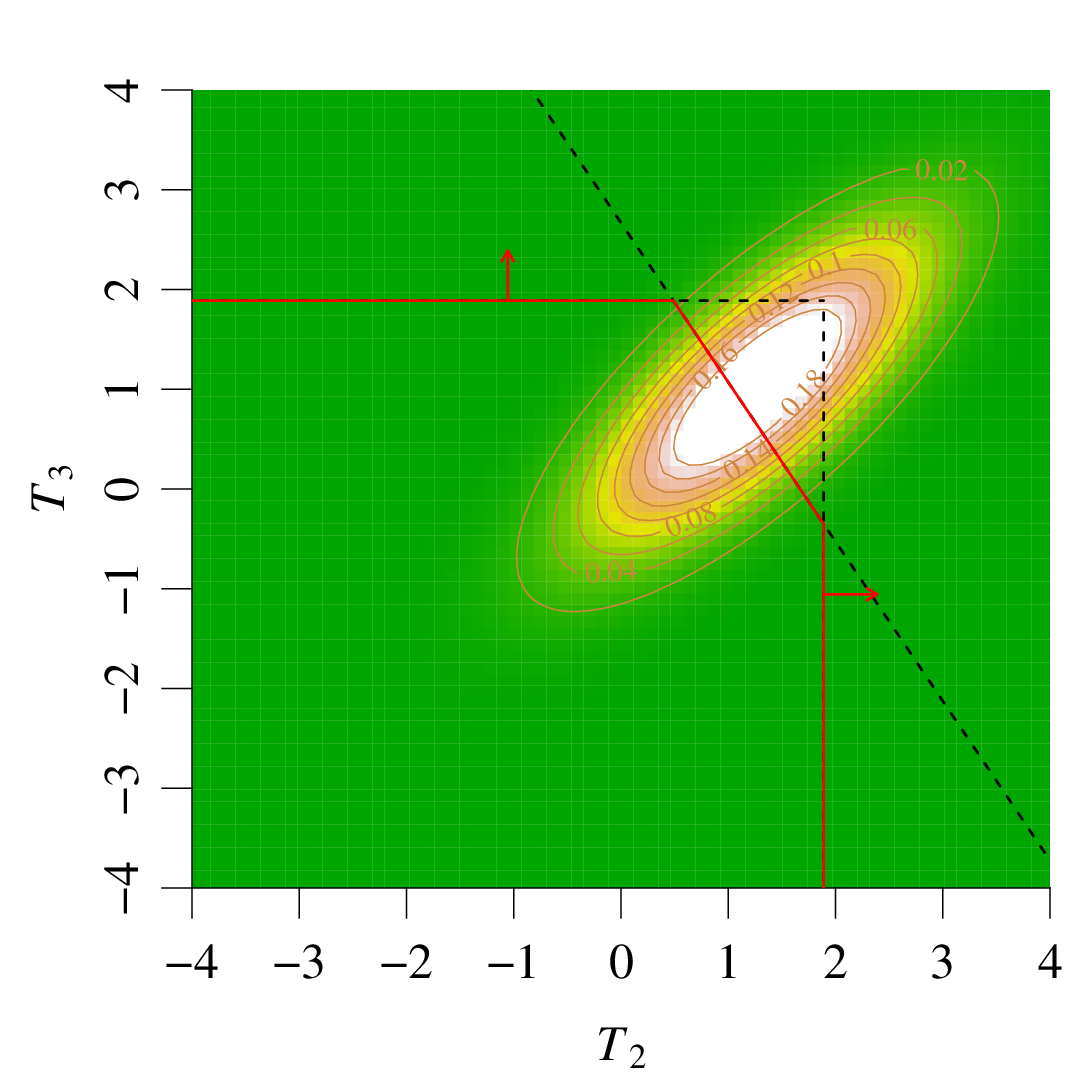
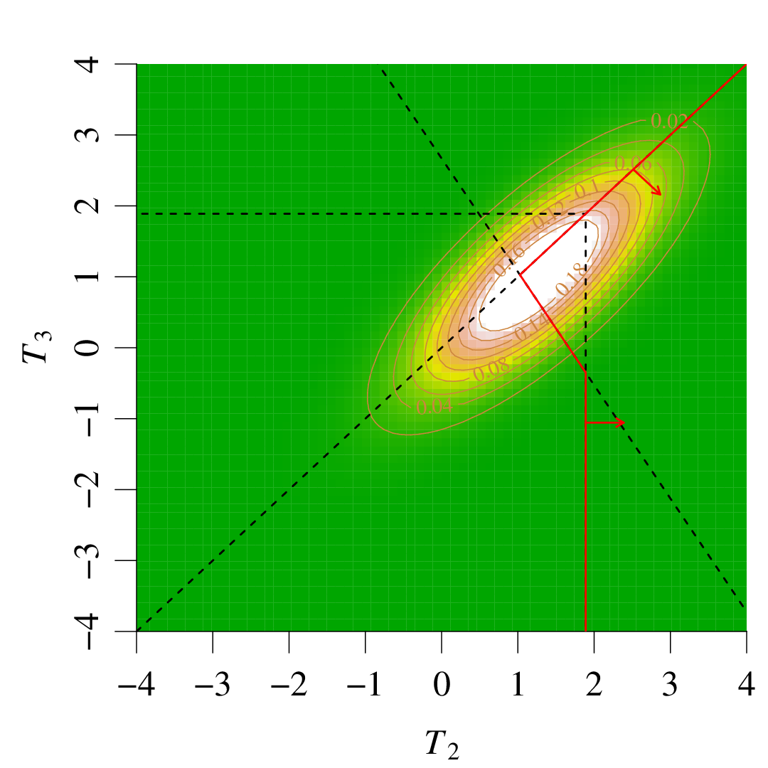
Supplemental Figures S2 and S2 show the contour plots and rejection regions of both statistics. Since the rank of the contrast coefficient matrix equals 2, the statistics , , and are linearly dependent random variables. Furthermore, the statistic is expressed by the equation:
.

.
| MAF | Method | (i) additive | (ii) dominant | (iii) recessive | ||||
|---|---|---|---|---|---|---|---|---|
| 0.12 | 1.83 | 1.83 | 1.83 | 78 | 20 | 2 | ||
| 1.93 | 1.67 | 3.08 | ||||||
| 0.25 | 1.89 | 1.89 | 1.89 | 56 | 37 | 7 | ||
| 1.91 | 1.69 | 2.70 | ||||||
| 0.33 | 1.91 | 1.91 | 1.91 | 44 | 44 | 12 | ||
| 1.89 | 1.73 | 2.40 | ||||||
| 0.50 | 1.93 | 1.93 | 1.93 | 25 | 50 | 25 | ||
| 1.87 | 1.95 | 1.95 | ||||||
| Abbreviation: MAF, minor allele frequency. Shaded region shows the smaller | ||||||||
| critical value from two methods. | ||||||||
Thus, it is apparent that the power for the modified maximum contrast method is higher than that for the maximum contrast method, as shown in Supplemental Figures S2 and S2, and in Equation 13.
Supplemental Table S1 shows other examples of the critical values and with a , and . In general, if the element of is smaller than the element of , then the power of the modified maximum contrast method is superior to that of the maximum contrast method in regard to the true response pattern, as shown in Equation 11. For instance, as shown in Supplemental Table S1, in the case of , if the true response pattern is the (i) additive, then the modified maximum contrast method is superior to the maximum contrast method (1.91 vs. 1.89, respectively); if the true response pattern is the (ii) dominant, then the modified maximum contrast method is again superior to the maximum contrast method (1.91 vs. 1.73, respectively); if the true response pattern is the (iii) recessive, then the modified method is instead inferior to the maximum contrast method (1.91 vs. 2.40, respectively).
Next, we consider the numerical example of and with , , and the (ii) dominant pattern with (; ). From Equation 12,
| (14) |
using Monte-Carlo integration. Supplemental Figures S4 and S4 show contour plots and integrating regions of both statistics.

| MAF | True response pattern | non-central parameter vector () | ||
|---|---|---|---|---|
| (i) additive | (ii) dominant | (iii) recessive | ||
| 0.12 | (i) additive | 0.70 | 0.52 | 0.97 |
| (ii) dominant | 0.70 | 0.70 | 0.64 | |
| (iii) recessive | 0.70 | 0.35 | 1.29 | |
| 0.25 | (i) additive | 1.25 | 0.96 | 1.53 |
| (ii) dominant | 1.25 | 1.27 | 1.02 | |
| (iii) recessive | 1.25 | 0.64 | 2.04 | |
| 0.33 | (i) additive | 1.54 | 1.22 | 1.69 |
| (ii) dominant | 1.54 | 1.62 | 1.13 | |
| (iii) recessive | 1.54 | 0.81 | 2.25 | |
| 0.50 | (i) additive | 1.77 | 1.60 | 1.60 |
| (ii) dominant | 1.77 | 2.13 | 1.07 | |
| (iii) recessive | 1.77 | 1.07 | 2.13 | |
| Shaded region shows the highest absolute value of the element of the non-central parameter vector. | ||||
Supplemental Table S2 shows the relationship between the true response patterns and the non-central parameter vectors. We considered true response patterns that were (i) additive, (ii) dominant pattern, and (iii) recessive with and a , and 0.50.
The element of the non-contral parameter vector that corresponds to the true response pattern must be the highest value in order to achieve a high ; however, as shown in Supplemental Table S2, this requirement is not satisfied when the MAF equals 0.12, 0.25, or 0.33. For example, in the case of , if the true response pattern is (i) additive, then the element of the (iii) recessive pattern is the highest value (0.97).
On the other hand, the modified maximum contrast method gives priority to ((i) additive) or ((ii) dominant) when the MAF is equal to 0.12, 0.25, or 0.33, as shown in Supplemental Table S1. In other words, this method adjusts the lower value of the non-contral parameter shown in Supplemental Table S2 ((i) additive and (ii) dominant). Therefore, is expected to be higher than with the (i) additive and (ii) dominant pattern in the conditions that are similar to those of actual pharmacogenomic studies.
Appendix B The simultaneous distribution of the proposed statistic
Now, we derive the simultaneous distribution of and show that does not depend on . As , follows -variate normal distribution , where is population mean vector and either singular or non-singular covariance matrix is
Statistic can be written as according to Equation 8, where is independently and follows a chi-square distribution with degrees of freedom. Thus, the joint distribution of is
| (15) |
Consider the transformation and the inverse transformation . The Jacobian of the transformation is
Note that is equal to 0 in the calculation. Thus, the joint distribution of is
| (16) |
Thus, the distribution of is obtained from Equations 15 and 16 by integrating out ,
| (17) |
Finally, under the overall null hypothesis, holds, then holds. Thus, Equation 17 becomes
Therefore, follows -variate -distribution under the overall null hypothesis.
Appendix C Supplemental tables
| MAF | Method | ||
|---|---|---|---|
| 0.12 | MCM | 0.050 | 0.049 |
| MMCM | 0.051 | 0.049 | |
| KW | 0.039 | 0.048 | |
| 0.25 | MCM | 0.049 | 0.052 |
| MMCM | 0.049 | 0.051 | |
| KW | 0.047 | 0.050 | |
| 0.33 | MCM | 0.051 | 0.049 |
| MMCM | 0.051 | 0.050 | |
| KW | 0.050 | 0.049 | |
| 0.50 | MCM | 0.049 | 0.051 |
| MMCM | 0.048 | 0.051 | |
| KW | 0.047 | 0.049 | |
| Abbreviations: MAF, minor allele frequency; MCM, maximum contrast method; MMCM, modified maxi- mum contrast method; KW, Kruskal–Wallis test. | |||
| = 0.25 | = 0.50 | = 1.00 | ||||||||||||
| MAF | True situation | Method | (i) | (ii) | (iii) | (i) | (ii) | (iii) | (i) | (ii) | (iii) | |||
| 0.12 |
(i) additive
![[Uncaptioned image]](2012.03475v1/type-a.png)
|
MCM | 0.010 | 0.018 | 0.041 | 0.069 | 0.012 | 0.015 | 0.102 | 0.129 | 0.014 | 0.005 | 0.398 | 0.417 |
| MMCM | 0.004 | 0.055 | 0.000 | 0.058 | 0.011 | 0.070 | 0.000 | 0.081 | 0.088 | 0.109 | 0.000 | 0.197 | ||
| KW | – | – | – | 0.058 | – | – | – | 0.132 | – | – | – | 0.484 | ||
(ii) dominant
![[Uncaptioned image]](2012.03475v1/type-b.png)
|
MCM | 0.011 | 0.026 | 0.027 | 0.064 | 0.018 | 0.045 | 0.039 | 0.103 | 0.058 | 0.120 | 0.091 | 0.270 | |
| MMCM | 0.002 | 0.060 | 0.000 | 0.062 | 0.002 | 0.104 | 0.000 | 0.106 | 0.004 | 0.271 | 0.000 | 0.275 | ||
| KW | – | – | – | 0.040 | – | – | – | 0.053 | – | – | – | 0.105 | ||
(iii) recessive
![[Uncaptioned image]](2012.03475v1/type-c.png)
|
MCM | 0.007 | 0.014 | 0.062 | 0.083 | 0.005 | 0.008 | 0.196 | 0.208 | 0.000 | 0.002 | 0.664 | 0.666 | |
| MMCM | 0.005 | 0.049 | 0.000 | 0.054 | 0.029 | 0.044 | 0.000 | 0.074 | 0.161 | 0.011 | 0.031 | 0.203 | ||
| KW | – | – | – | 0.116 | – | – | – | 0.399 | – | – | – | 0.954 | ||
| 0.25 |
(i) additive
|
MCM | 0.021 | 0.020 | 0.062 | 0.104 | 0.046 | 0.021 | 0.211 | 0.278 | 0.066 | 0.008 | 0.727 | 0.801 |
| MMCM | 0.020 | 0.062 | 0.001 | 0.083 | 0.083 | 0.092 | 0.006 | 0.181 | 0.438 | 0.115 | 0.054 | 0.607 | ||
| KW | – | – | – | 0.090 | – | – | – | 0.243 | – | – | – | 0.760 | ||
|
(ii) dominant
|
MCM | 0.020 | 0.038 | 0.032 | 0.089 | 0.061 | 0.114 | 0.053 | 0.228 | 0.205 | 0.390 | 0.083 | 0.678 | |
| MMCM | 0.010 | 0.083 | 0.000 | 0.093 | 0.022 | 0.224 | 0.000 | 0.246 | 0.045 | 0.668 | 0.000 | 0.713 | ||
| KW | – | – | – | 0.075 | – | – | – | 0.168 | – | – | – | 0.550 | ||
|
(iii) recessive
|
MCM | 0.014 | 0.012 | 0.110 | 0.136 | 0.010 | 0.004 | 0.425 | 0.438 | 0.000 | 0.000 | 0.969 | 0.970 | |
| MMCM | 0.033 | 0.040 | 0.003 | 0.075 | 0.116 | 0.022 | 0.050 | 0.188 | 0.196 | 0.001 | 0.616 | 0.812 | ||
| KW | – | – | – | 0.171 | – | – | – | 0.556 | – | – | – | 0.994 | ||
| 0.33 |
(i) additive
|
MCM | 0.030 | 0.026 | 0.060 | 0.116 | 0.089 | 0.037 | 0.215 | 0.342 | 0.199 | 0.020 | 0.672 | 0.891 |
| MMCM | 0.038 | 0.058 | 0.005 | 0.102 | 0.149 | 0.103 | 0.028 | 0.279 | 0.609 | 0.106 | 0.110 | 0.824 | ||
| KW | – | – | – | 0.099 | – | – | – | 0.274 | – | – | – | 0.831 | ||
|
(ii) dominant
|
MCM | 0.030 | 0.054 | 0.029 | 0.113 | 0.087 | 0.192 | 0.041 | 0.320 | 0.223 | 0.610 | 0.029 | 0.862 | |
| MMCM | 0.025 | 0.095 | 0.002 | 0.122 | 0.053 | 0.302 | 0.001 | 0.357 | 0.072 | 0.818 | 0.000 | 0.890 | ||
| KW | – | – | – | 0.093 | – | – | – | 0.255 | – | – | – | 0.791 | ||
|
(iii) recessive
|
MCM | 0.020 | 0.014 | 0.124 | 0.159 | 0.022 | 0.004 | 0.489 | 0.515 | 0.001 | 0.000 | 0.987 | 0.988 | |
| MMCM | 0.050 | 0.033 | 0.020 | 0.103 | 0.145 | 0.014 | 0.172 | 0.332 | 0.151 | 0.001 | 0.804 | 0.955 | ||
| KW | – | – | – | 0.172 | – | – | – | 0.556 | – | – | – | 0.993 | ||
| 0.50 |
(i) additive
|
MCM | 0.041 | 0.045 | 0.045 | 0.132 | 0.155 | 0.120 | 0.117 | 0.392 | 0.529 | 0.195 | 0.199 | 0.923 |
| MMCM | 0.062 | 0.035 | 0.035 | 0.132 | 0.226 | 0.088 | 0.084 | 0.398 | 0.692 | 0.116 | 0.119 | 0.927 | ||
| KW | – | – | – | 0.104 | – | – | – | 0.304 | – | – | – | 0.864 | ||
|
(ii) dominant
|
MCM | 0.034 | 0.095 | 0.020 | 0.149 | 0.079 | 0.392 | 0.013 | 0.483 | 0.049 | 0.928 | 0.000 | 0.977 | |
| MMCM | 0.053 | 0.080 | 0.015 | 0.148 | 0.127 | 0.346 | 0.007 | 0.480 | 0.101 | 0.875 | 0.000 | 0.977 | ||
| KW | – | – | – | 0.137 | – | – | – | 0.443 | – | – | – | 0.968 | ||
|
(iii) recessive
|
MCM | 0.035 | 0.019 | 0.102 | 0.156 | 0.077 | 0.014 | 0.388 | 0.480 | 0.043 | 0.000 | 0.935 | 0.978 | |
| MMCM | 0.056 | 0.013 | 0.087 | 0.156 | 0.125 | 0.008 | 0.345 | 0.478 | 0.098 | 0.000 | 0.879 | 0.977 | ||
| KW | – | – | – | 0.144 | – | – | – | 0.439 | – | – | – | 0.967 | ||
| Abbreviations: MAF, minor allele frequency; MCM, maximum contrast method; MMCM, modified maximum contrast method; KW, Kruskal–Wallis test. Shaded region shows positive predictive value () for detection of true response patterns. | ||||||||||||||
| = 0.25 | = 0.50 | = 1.00 | ||||||||||||
| MAF | True situation | Method | (i) | (ii) | (iii) | (i) | (ii) | (iii) | (i) | (ii) | (iii) | |||
| 0.12 |
(i) additive
|
MCM | 0.010 | 0.015 | 0.073 | 0.098 | 0.013 | 0.007 | 0.273 | 0.293 | 0.001 | 0.000 | 0.834 | 0.835 |
| MMCM | 0.005 | 0.063 | 0.000 | 0.068 | 0.043 | 0.100 | 0.000 | 0.143 | 0.381 | 0.094 | 0.005 | 0.480 | ||
| KW | – | – | – | 0.121 | – | – | – | 0.392 | – | – | – | 0.942 | ||
|
(ii) dominant
|
MCM | 0.015 | 0.035 | 0.033 | 0.083 | 0.036 | 0.081 | 0.070 | 0.188 | 0.135 | 0.273 | 0.179 | 0.587 | |
| MMCM | 0.001 | 0.083 | 0.000 | 0.084 | 0.002 | 0.190 | 0.000 | 0.192 | 0.006 | 0.590 | 0.000 | 0.596 | ||
| KW | – | – | – | 0.064 | – | – | – | 0.131 | – | – | – | 0.424 | ||
|
(iii) recessive
|
MCM | 0.004 | 0.010 | 0.133 | 0.147 | 0.000 | 0.003 | 0.477 | 0.481 | 0.000 | 0.001 | 0.977 | 0.977 | |
| MMCM | 0.015 | 0.047 | 0.000 | 0.062 | 0.109 | 0.020 | 0.004 | 0.134 | 0.220 | 0.001 | 0.454 | 0.676 | ||
| KW | – | – | – | 0.321 | – | – | – | 0.887 | – | – | – | 1.000 | ||
| 0.25 |
(i) additive
|
MCM | 0.035 | 0.021 | 0.154 | 0.210 | 0.059 | 0.011 | 0.589 | 0.659 | 0.008 | 0.000 | 0.990 | 0.998 |
| MMCM | 0.055 | 0.085 | 0.002 | 0.141 | 0.306 | 0.124 | 0.024 | 0.454 | 0.850 | 0.031 | 0.100 | 0.981 | ||
| KW | – | – | – | 0.193 | – | – | – | 0.629 | – | – | – | 0.997 | ||
|
(ii) dominant
|
MCM | 0.041 | 0.080 | 0.046 | 0.167 | 0.150 | 0.289 | 0.085 | 0.523 | 0.326 | 0.613 | 0.043 | 0.982 | |
| MMCM | 0.013 | 0.166 | 0.000 | 0.179 | 0.037 | 0.516 | 0.000 | 0.553 | 0.014 | 0.971 | 0.000 | 0.986 | ||
| KW | – | – | – | 0.129 | – | – | – | 0.419 | – | – | – | 0.958 | ||
|
(iii) recessive
|
MCM | 0.010 | 0.005 | 0.316 | 0.331 | 0.000 | 0.001 | 0.892 | 0.893 | 0.000 | 0.000 | 1.000 | 1.000 | |
| MMCM | 0.085 | 0.026 | 0.018 | 0.129 | 0.211 | 0.003 | 0.386 | 0.600 | 0.078 | 0.000 | 0.922 | 1.000 | ||
| KW | – | – | – | 0.450 | – | – | – | 0.971 | – | – | – | 1.000 | ||
| 0.33 |
(i) additive
|
MCM | 0.071 | 0.034 | 0.169 | 0.275 | 0.173 | 0.027 | 0.583 | 0.783 | 0.096 | 0.000 | 0.904 | 1.000 |
| MMCM | 0.108 | 0.094 | 0.018 | 0.220 | 0.478 | 0.121 | 0.087 | 0.686 | 0.909 | 0.023 | 0.067 | 0.999 | ||
| KW | – | – | – | 0.230 | – | – | – | 0.712 | – | – | – | 1.000 | ||
|
(ii) dominant
|
MCM | 0.066 | 0.136 | 0.042 | 0.244 | 0.207 | 0.489 | 0.040 | 0.736 | 0.188 | 0.810 | 0.002 | 1.000 | |
| MMCM | 0.043 | 0.226 | 0.001 | 0.271 | 0.074 | 0.703 | 0.001 | 0.777 | 0.011 | 0.989 | 0.000 | 1.000 | ||
| KW | – | – | – | 0.201 | – | – | – | 0.658 | – | – | – | 0.999 | ||
|
(iii) recessive
|
MCM | 0.022 | 0.005 | 0.379 | 0.406 | 0.003 | 0.000 | 0.946 | 0.949 | 0.000 | 0.000 | 1.000 | 1.000 | |
| MMCM | 0.121 | 0.019 | 0.099 | 0.239 | 0.182 | 0.001 | 0.670 | 0.853 | 0.038 | 0.000 | 0.962 | 1.000 | ||
| KW | – | – | – | 0.449 | – | – | – | 0.969 | – | – | – | 1.000 | ||
| 0.50 |
(i) additive
|
MCM | 0.115 | 0.096 | 0.102 | 0.312 | 0.437 | 0.200 | 0.202 | 0.839 | 0.817 | 0.090 | 0.093 | 1.000 |
| MMCM | 0.169 | 0.071 | 0.077 | 0.317 | 0.589 | 0.127 | 0.129 | 0.845 | 0.945 | 0.028 | 0.028 | 1.000 | ||
| KW | – | – | – | 0.244 | – | – | – | 0.761 | – | – | – | 1.000 | ||
|
(ii) dominant
|
MCM | 0.072 | 0.290 | 0.016 | 0.379 | 0.065 | 0.865 | 0.002 | 0.932 | 0.002 | 0.998 | 0.000 | 1.000 | |
| MMCM | 0.112 | 0.255 | 0.010 | 0.377 | 0.123 | 0.806 | 0.001 | 0.930 | 0.016 | 0.985 | 0.000 | 1.000 | ||
| KW | – | – | – | 0.351 | – | – | – | 0.915 | – | – | – | 1.000 | ||
|
(iii) recessive
|
MCM | 0.068 | 0.014 | 0.300 | 0.382 | 0.064 | 0.002 | 0.867 | 0.933 | 0.002 | 0.000 | 0.998 | 1.000 | |
| MMCM | 0.106 | 0.009 | 0.264 | 0.379 | 0.124 | 0.001 | 0.807 | 0.931 | 0.013 | 0.000 | 0.987 | 1.000 | ||
| KW | – | – | – | 0.354 | – | – | – | 0.917 | – | – | – | 1.000 | ||
| Abbreviations: MAF, minor allele frequency; MCM, maximum contrast method; MMCM, modified maximum contrast method; KW, Kruskal–Wallis test. Shaded region shows positive predictive value () for detection of true response patterns. | ||||||||||||||
| MAF | Response pattern | ||||
|---|---|---|---|---|---|
| 0.12 |
(iv) valley
![[Uncaptioned image]](2012.03475v1/type-d.png)
|
MCM | 0.066 | 0.103 | 0.273 |
| MMCM | 0.055 | 0.064 | 0.119 | ||
| KW | 0.118 | 0.380 | 0.936 | ||
| 0.25 |
(iv) valley
|
MCM | 0.082 | 0.183 | 0.604 |
| MMCM | 0.062 | 0.111 | 0.363 | ||
| KW | 0.161 | 0.537 | 0.989 | ||
| 0.33 |
(iv) valley
|
MCM | 0.091 | 0.223 | 0.742 |
| MMCM | 0.076 | 0.164 | 0.608 | ||
| KW | 0.170 | 0.560 | 0.993 | ||
| 0.50 |
(iv) valley
|
MCM | 0.095 | 0.248 | 0.804 |
| MMCM | 0.091 | 0.238 | 0.792 | ||
| KW | 0.173 | 0.559 | 0.994 | ||
| Abbreviations: MAF, minor allele frequency; MCM, maximum contrast method; MMCM, modified maximum contrast method; KW, Kruskal–Wallis test. Shaded region is minimum false positive rate at each MAF and . | |||||
| MAF | Response pattern | ||||
|---|---|---|---|---|---|
| 0.12 |
(iv) valley
|
MCM | 0.091 | 0.198 | 0.629 |
| MMCM | 0.062 | 0.091 | 0.245 | ||
| KW | 0.306 | 0.869 | 1.000 | ||
| 0.25 |
(iv) valley
|
MCM | 0.147 | 0.455 | 0.996 |
| MMCM | 0.091 | 0.247 | 0.944 | ||
| KW | 0.425 | 0.964 | 1.000 | ||
| 0.33 |
(iv) valley
|
MCM | 0.175 | 0.584 | 1.000 |
| MMCM | 0.128 | 0.439 | 0.999 | ||
| KW | 0.448 | 0.968 | 1.000 | ||
| 0.50 |
(iv) valley
|
MCM | 0.197 | 0.664 | 1.000 |
| MMCM | 0.190 | 0.648 | 1.000 | ||
| KW | 0.452 | 0.971 | 1.000 | ||
| Abbreviations: MAF, minor allele frequency; MCM, maximum contrast method; MMCM, modified maximum contrast method; KW, Kruskal–Wallis test. Shaded region is minimum false positive rate at each MAF and . | |||||