跳到论文正文
W Papers独立论文阅读器 arXiv:2012.03467 论文正文 计算阅读时间 · 0%
引用这篇论文根据当前论文元数据生成,正式投稿前建议核对。


License: CC BY 4.0
arXiv:2012.03467v2 [math.PR] 11 Nov 2022

Hyperbolic Radial Spanning TreeAcknowledgments. This work has been supported by the LAMAV (Université Polytechnique des Hauts de France) and the Laboratoire P. Painlevé (Université de Lille). It has also benefitted from the GdR GeoSto 3477 from CNRS, the Labex CEMPI (ANR-11-LABX-0007-01), the Labex Bézout (ANR-10-LABX-0058) and the ANR PPPP (ANR-16-CE40-0016).

David Coupier Note: Institut Mines Télécom Nord Europe, F-59650 Villeneuve d’Ascq, France david.coupier@imt-nord-europe.fr    Lucas Flammant  and  Viet Chi Tran Note: Univ. de Valenciennes, CNRS, EA 4015 - LAMAV, F-59313 Valenciennes Cedex 9, France Note: LAMA, Univ Gustave Eiffel, Univ Paris Est Creteil, CNRS, F-77454 Marne-la-Vallée, France; IRL 3457, CRM-CNRS, Université de Montréal, Canada. chi.tran@univ-eiffel.fr
August 11, 2026
Abstract

We define and analyze an extension to the dd-dimensional hyperbolic space of the Radial Spanning Tree (RST) introduced by Baccelli and Bordenave in the two-dimensional Euclidean space (2007). In particular, we will focus on the description of the infinite branches of the tree. The properties of the two-dimensional Euclidean RST are extended to the hyperbolic case in every dimension: almost surely, every infinite branch admits an asymptotic direction and each asymptotic direction is reached by at least one infinite branch. Moreover, the branch converging to any deterministic asymptotic direction is unique almost surely. To obtain results for any dimension, a completely new approach is considered here. Our strategy mainly involves the two following ingredients, that rely on the hyperbolic Directed Spanning Forest (DSF) introduced and studied in Flammant (2019). First, the hyperbolic metric allows us to obtain fine control of the branches’ fluctuations in the hyperbolic DSF without using planarity arguments. Then, we couple the hyperbolic RST with the hyperbolic DSF and conclude.

Key words: continuum percolation, hyperbolic space, stochastic geometry, random geometric tree, Radial Spanning Tree, Directed Spanning Forest, Poisson point processes.

AMS 2010 Subject Classification: Primary 60D05, 60K35, 82B21.

1 Introduction

Geometric random trees are well studied in the literature since they interact with many other fields, such as communication networks, particles systems or population dynamics. Several works have established scaling limits for two-dimensional radial trees [10, 9] and translation invariant forests [11, 26, 15]. In addition, random spanning trees appear in the context of first passage percolation [16]. A complete introduction to geometric random graphs is given in Penrose [22].

Here we are interested in the Radial Spanning Tree (RST), introduced by Baccelli and Bordenave [1] in the Euclidean plane and with motivations from communication networks. The construction of this tree is the same on the plane ℝ2\mathbb{R}^{2} or on the hyperbolic space ℍd+1\mathbb{H}^{d+1} (presented below). The set of vertices is given by a homogeneous Poisson Point Process (PPP) 𝒩\mathcal{N} of intensity λ\lambda. The RST rooted at the origin 00 is the graph obtained by connecting each point z∈𝒩z\in\mathcal{N} to its parent A⁡(z)A(z), defined as the closest point to zz among all points z′∈𝒩∪{0}z^{\prime}\in\mathcal{N}\cup\{0\} that are closer to the origin than zz. This defines a random tree rooted at the origin with a radial structure. Given a path, we will say that the forward direction is towards 00 and the backward direction is towards infinity. An infinite backward path is defined as a sequence of Poisson points (zn)n≥0∈(𝒩∪{0})ℕ(z_{n})_{n\geq 0}\in\left(\mathcal{N}\cup\{0\}\right)^{\mathbb{N}} with z0=0z_{0}=0 and zn=A⁡(zn+1)z_{n}=A(z_{n+1}) for any n≥0n\geq 0. Because a vertex can be the ancestor of no other vertex, all backward paths are not infinite.

The topological properties of the bi-dimensional Euclidean RST are well-understood. Baccelli and Bordenave showed that almost surely (a.s.), any infinite backward path admits an asymptotic direction, i.e. that a.s. for any infinite path (zn)n≥0(z_{n})_{n\geq 0}, the sequence (zn/|zn|)n≥0(z_{n}/|z_{n}|)_{n\geq 0} converges to a limit in the unit sphere 𝕊1\mathbb{S}^{1} of ℝ2\mathbb{R}^{2}. The limit is called the asymptotic direction of the infinite path. Moreover, a.s., every asymptotic direction of 𝕊1\mathbb{S}^{1} is reached by at least one infinite backward path and there exists a.s. a unique infinite path in any given deterministic asymptotic direction [1]. These results on the infinite paths are completed by Baccelli, Coupier & Tran [2].

For any integer d≥1d\geq 1, the hyperbolic space ℍd+1\mathbb{H}^{d+1} is a (d+1)(d+1)-dimensional Riemannian manifold with constant negative curvature, that can be chosen equal to −1-1 without loss of generality. It admits a set of ideal boundary points ∂ℍd+1\partial\mathbb{H}^{d+1}, and ℍd+1¯:=ℍd+1∪∂ℍd+1\overline{\mathbb{H}^{d+1}}:=\mathbb{H}^{d+1}\cup\partial\mathbb{H}^{d+1} denotes the hyperbolic space endowed with its boundary. It is a non-amenable space, i.e. the measure of the boundary of a large subset is not negligible with respect to its volume. The hyperbolic space is defined in more details in [7, 8, 21, 25].

There is a growing interest for the study of random models in a hyperbolic setting. Benjamini and Schramm establish percolation results on regular tilings and Voronoï tessellations in the hyperbolic plane [3]. Mean characteristics of the Poisson-Voronoï tessellation have also been considered in a general Riemannian manifold by Calka et al. [6]. This interest is explained by at least two reasons. First, hyperbolic random graphs are well-fitted to model social networks [5]. Secondly, strong differences have been noticed for properties of random models depending on whether they are considered in an Euclidean or in a hyperbolic setting. For example, some hyperbolic random graphs admit a non-degenerate regime with infinitely many unbounded components in the hyperbolic space [27, 17], which is generally not the case in the Euclidean space. In addition, behaviors of non-amenable spaces are well studied in a discrete context [4, 19, 23].

Thus it is natural to consider and study the hyperbolic RST, which we define in the same way as the Euclidean RST. A simulation of the two-dimensional hyperbolic RST is given in Figure 1. In this paper, we extend the results of Baccelli and his coauthors to hyperbolic geometry in every dimension. Here is our main result:

Theorem 1.1.

For any dimension d≥1d\geq 1 and any intensity λ\lambda, the following happens:

  1. (i)

    almost surely, any infinite backward path (zn)n∈ℕ(z_{n})_{n\in\mathbb{N}} admits an asymptotic direction, i.e. there exists z∞∈∂ℍd+1z_{\infty}\in\partial\mathbb{H}^{d+1} such that limn→∞zn=z∞\lim_{n\to\infty}z_{n}=z_{\infty} (in the sense of the topology of ℍd+1¯\overline{\mathbb{H}^{d+1}});

  2. (ii)

    almost surely, for any z∞∈∂ℍd+1z_{\infty}\in\partial\mathbb{H}^{d+1}, there exists an infinite backward path (zn)(z_{n}) with asymptotic direction z∞z_{\infty};

  3. (iii)

    for any deterministic boundary point z∞∈∂ℍd+1z_{\infty}\in\partial\mathbb{H}^{d+1}, the path with asymptotic direction z∞z_{\infty} is almost surely unique;

  4. (iv)

    the set of boundary points with at least two infinite backward paths is dense in ∂ℍd+1\partial\mathbb{H}^{d+1};

  5. (v)

    this set is moreover countable in the bi-dimensional case (i.e. d=1d=1).

Theorem 1.1 describes the infinite branches of the hyperbolic RST: every infinite branch admits an asymptotic direction and Point (ii) and (iii) say that for any fixed and deterministic boundary point II, there exists a unique infinite path having II as asymptotic direction. But there is a random dense set of boundary points having more than one backwards paths, and in dimension 2 (for d=1d=1) this set is countable.

Establishing the results announced in Theorem 1.1 in every dimension constitutes the main originality of this paper. For the two reasons explained further, the proofs of Baccelli and Bordenave in the 2D-Euclidean setting [1] cannot be generalized to higher dimensions.

In both contexts ℝ2\mathbb{R}^{2} and ℍd+1\mathbb{H}^{d+1}, for any d≥1d\geq 1, the proofs of (i), (ii), (iv) and (v) of Theorem 1.1 follow the strategy of Howard and Newman [16], which is to show that the tree is straight, that is, the descendant subtree of a vertex far from the origin is included in a thin cone. To prove that the 2D-Euclidean RST is straight, Baccelli and Bordenave used a translation invariant model derived from the RST: the Directed Spanning Forest (DSF), which constitutes a local approximation of the RST far from the origin [1]. They exploit the theory of Markov chains to bound from above fluctuations of trajectories in the DSF and then, they deduce the straightness of the RST via planarity. This strategy cannot be generalized to higher dimensions. However, in ℍd+1\mathbb{H}^{d+1}, we manage to control the angular deviations of branches in the RST without resorting to an auxiliary model, that requires planarity as in the Euclidean setting. The hyperbolic metric guarantees that angular deviations decay exponentially fast with the distance to the origin, which is strong enough to show straightness.

In addition, in the Euclidean context, the uniqueness part (point (iii) in Theorem 1.1) is only proved in dimension 22 since it strongly uses planarity [16, 1], and the strategy of proof cannot be generalized to higher dimensions. To prove (iii) in ℍd+1\mathbb{H}^{d+1}, our strategy consists in exploiting the link existing between the hyperbolic RST and the hyperbolic DSF, defined and studied in Flammant 2019 [12], which is the hyperbolic counterpart of the Euclidean DSF used by Baccelli and Bordenave. Roughly speaking, the hyperbolic DSF can be defined as the limit of the hyperbolic RST when the origin point tends to an ideal boundary point. Similarly to the Euclidean setting, it constitutes a local approximation of the RST far from the origin. The proof of (iii) exploits the coalescence of the hyperbolic DSF (i.e. it is almost surely a tree) [12, Theorem 1.1], which is a non-trivial fact obtained by exploiting the mass-transport principle, and a local coupling between the two models.

After defining the hyperbolic RST and giving its basic properties, we define two quantities that encode angular fluctuations along trajectories, the Cumulative angular Forward Deviations (CFD) and the Maximal Backward Deviations (MBD). We then establish upper bounds of these quantities: first, we upper-bound the Maximal Backward Deviations in a thin annulus of width δ>0\delta>0 (Proposition 2.5) and then we deduce a global control of MBD in the whole space (Proposition 2.6), that roughly says that angular deviations decay exponentially fast with the distance to the origin. From this upper-bound, we deduce that the RST is straight in the sense of Howard & Newman (Proposition 2.7). The points (i), (ii), (iv) and (v) in Theorem 1.1 can be deduced from straightness and the upper-bound of MBD given by Proposition 2.6. The point (iii) (the uniqueness part) is done by exploiting a local coupling existing between the RST and the DSF far from the origin.

The rest of paper is organized as follows. In Section 2, we set some reminders of hyperbolic geometry and we define the hyperbolic RST. Then, we give its basic properties and a road-map of the proofs. We also announce the upper bounds of angular deviations (Propositions 2.5 and 2.6) and the straightness property (Proposition 2.7). The proof of Theorem 1.1 is done in Section 3. Proposition 2.5 is proved in Section 4 and the proofs of Propositions 2.6 and 2.7 are done in Section 5.

Refer to caption
Figure 1: Simulation of the two-dimensional hyperbolic RST, with λ=30\lambda=30, in the Poincaré disc model. The edges are represented by geodesics. The different connected components of the RST (apart from the root) are represented with different colors.

2 Definitions, notations and basic properties

We denote by ℕ\mathbb{N} the set of non-negative integers and by ℕ∗\mathbb{N}^{*} the set of positive integers. In the rest of the paper, cc (resp. CC) will be some small (resp. large) constant whose value can change from a line to another.

2.1 The hyperbolic space

We refer to [25] for a complete introduction to hyperbolic geometry. For d∈ℕ∗d\in\mathbb{N}^{*}, the (d+1)(d+1)-dimensional hyperbolic space, denoted by ℍd+1\mathbb{H}^{d+1}, is a (d+1)(d+1)-dimensional Riemannian manifold of constant negative curvature −1-1 that can be defined by several isometric models. One of them is the open-ball model consisting in the unit open ball

I={(x1,…,xd+1)∈ℝd+1,x12+…+xd+12<1}\displaystyle I=\{(x_{1},...,x_{d+1})\in\mathbb{R}^{d+1},~x_{1}^{2}+...+x_{d+1}^{2}<1\} (2.1)

endowed with the following metric:

d​sI2:=4​d​x12+…+d​xd+12(1−x12−…−xd+12)2.\displaystyle ds_{I}^{2}:=4\frac{dx_{1}^{2}+...+dx_{d+1}^{2}}{(1-x_{1}^{2}-...-x_{d+1}^{2})^{2}}. (2.2)

We denote by d⁡(⋅,⋅)d(\cdot,\cdot) the hyperbolic distance in ℍd+1\mathbb{H}^{d+1}, and by ∥⋅∥\|\cdot\| the Euclidean norm in ℝd\mathbb{R}^{d}, with the convention ‖∞‖=∞\|\infty\|=\infty.

The volume measure on (I,d​sI2)(I,ds_{I}^{2}), denoted by VolI\mbox{Vol}_{I}, is given by

d​VolI=2d+1​d​x1​…​d​xd+1(1−x12−…−xd+12)d+1.\displaystyle d\mbox{Vol}_{I}=2^{d+1}\frac{dx_{1}...dx_{d+1}}{(1-x_{1}^{2}-...-x_{d+1}^{2})^{d+1}}. (2.3)

An important fact about hyperbolic geometry is that ℍd+1\mathbb{H}^{d+1} is homogeneous, isotropic and rotation invariant. It means that the group of isometries of ℍd+1\mathbb{H}^{d+1} acts transitively on the unit tangent bundle of ℍd+1\mathbb{H}^{d+1}: given two points x,y∈ℍd+1x,y\in\mathbb{H}^{d+1} and two unit tangent vectors u∈Tx​ℍd+1,v∈Ty​ℍd+1u\in T_{x}\mathbb{H}^{d+1},~v\in T_{y}\mathbb{H}^{d+1}, there exists an isometry gg of ℍd+1\mathbb{H}^{d+1} such that g⁡(x)=yg(x)=y and that pushes forward uu on vv. The notations TxT_{x}, TyT_{y} and the vocabulary relating to Riemannian geometry are defined in [18]. We refer to [21, Proposition 1.2.1 p.5] for a proof.

Let 0∈ℍd+10\in\mathbb{H}^{d+1} be some arbitrary origin point (it can be thought as the center of the ball in the open-ball representation), which will play the role of the root of the RST.
The hyperbolic space ℍd+1\mathbb{H}^{d+1} is naturally equipped with a set of points at infinity, denoted by ∂ℍd+1\partial\mathbb{H}^{d+1}. In the open-ball model (I,d​sI2)(I,ds_{I}^{2}), the set of points at infinity is identified by the boundary unit sphere. Let us denote by 𝕊d\mathbb{S}^{d} the unit Euclidean sphere in ℝd+1\mathbb{R}^{d+1} and by ν\nu its dd-dimensional volume measure. We denote by ℍd+1¯:=ℍd+1∪∂ℍd+1\overline{\mathbb{H}^{d+1}}:=\mathbb{H}^{d+1}\cup\partial\mathbb{H}^{d+1} the hyperbolic space ℍd+1\mathbb{H}^{d+1} plus the set of points at infinity, with the topology given by the closed ball. A point z∞∈∂ℍd+1z_{\infty}\in\partial\mathbb{H}^{d+1} is called ideal point or point at infinity.
The metric becomes smaller as we get closer to the boundary unit sphere ∂I\partial I, and this boundary is at infinite distance from the center 00.
For any subset E⊂ℍd+1¯E\subset\overline{\mathbb{H}^{d+1}}, E¯\overline{E} denotes the closure of EE in ℍd+1¯\overline{\mathbb{H}^{d+1}}.

In the open ball model (I,d​sI2)(I,ds_{I}^{2}), the geodesics are of two types: the diameters of II and the arcs that are perpendicular to the boundary unit sphere 𝕊d\mathbb{S}^{d}, see Figure 2. We refer to discussion [7, p.80] for a proof. This model is conformal, which means that the hyperbolic angle between two geodesics corresponds to their Euclidean angle in the open-ball representation. For z1,z2,z3∈ℍ¯d+1z_{1},z_{2},z_{3}\in\overline{\mathbb{H}}^{d+1}, z1​z2​z3^\widehat{z_{1}z_{2}z_{3}} is the measure of the corresponding (non-oriented) angle.
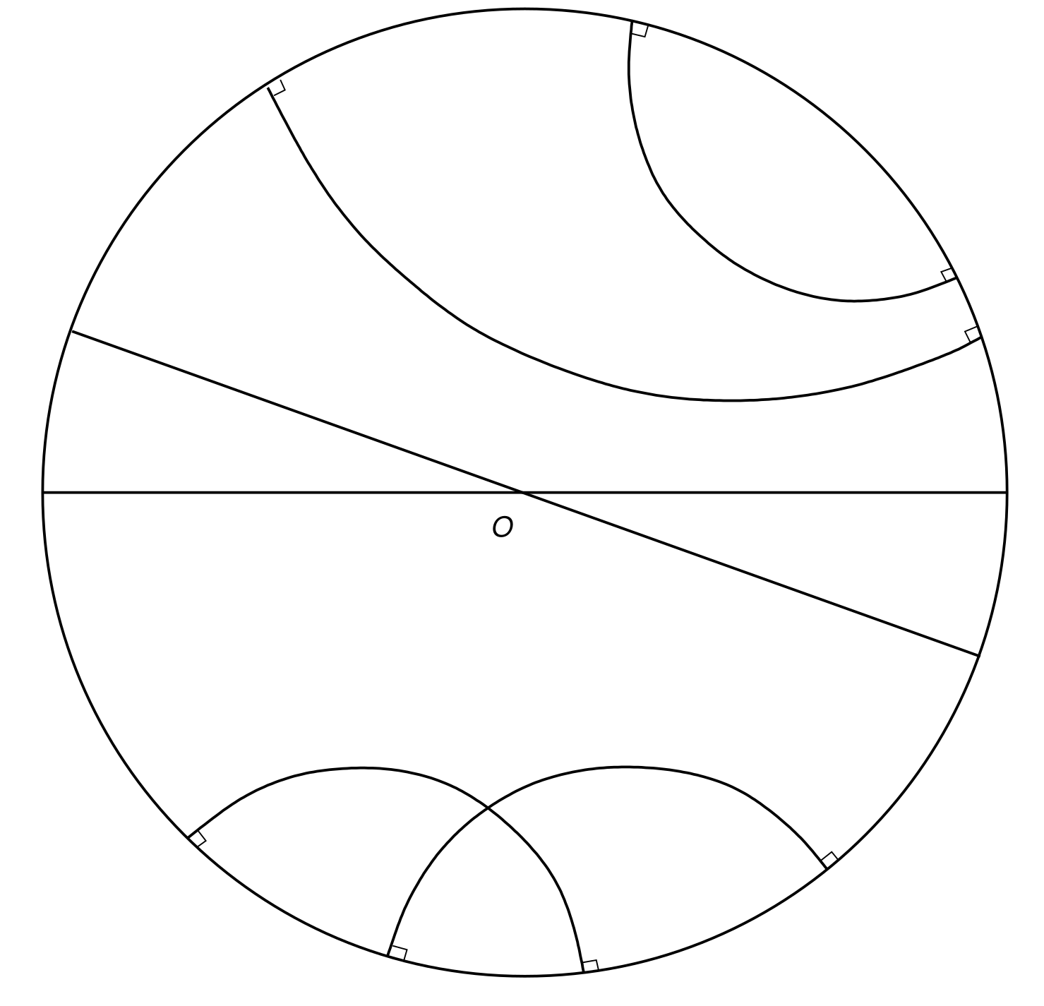
Refer to caption
Figure 2: Geodesics in the open ball model

For z1,z2∈ℍ¯d+1z_{1},z_{2}\in\overline{\mathbb{H}}^{d+1}, let us denote by [z1,z2][z_{1},z_{2}] the geodesic between z1z_{1} and z2z_{2}. Moreover, we set the notations:

[z1,z2[:=[z1,z2]\{z2},]z1,z2]:=[z1,z2]\{z1},]z1,z2[\({z2}∪{z2}).[z_{1},z_{2}[:=[z_{1},z_{2}]\backslash\{z_{2}\},\quad]z_{1},z_{2}]:=[z_{1},z_{2}]\backslash\{z_{1}\},\quad]z_{1},z_{2}[\backslash(\{z_{2}\}\cup\{z_{2}\}).

Let us denote by [z1,z2)[z_{1},z_{2}) (resp. (z1,z2](z_{1},z_{2}]) the semi-geodesic passing through z2z_{2} (resp. z1z_{1}) and ending at z1z_{1} (resp. z2z_{2}).

For z∈ℍd+1z\in\mathbb{H}^{d+1} and r>0r>0, we denote by B⁡(z,r):={z′∈H,d⁡(z,z′)<r}B(z,r):=\{z^{\prime}\in H,~d(z,z^{\prime})<r\} (resp. S⁡(z,r):={z′∈H,d⁡(z,z′)=r}S(z,r):=\{z^{\prime}\in H,~d(z,z^{\prime})=r\}) the hyperbolic ball (resp. s​p​h​e​r​esphere) centered at zz of radius rr, and we set B⁡(r):=B⁡(0,r)B(r):=B(0,r) (resp. S⁡(r):=S⁡(0,r)S(r):=S(0,r)). For x∈ℝdx\in\mathbb{R}^{d} and r>0r>0, let us also denote by Bℝd​(x,r):={x′∈ℝd,‖x′−x‖<r}B_{\mathbb{R}^{d}}(x,r):=\{x^{\prime}\in\mathbb{R}^{d},~\|x^{\prime}-x\|<r\} the Euclidean ball centered at xx of radius rr.
For any point z∈ℍd+1¯z\in\overline{\mathbb{H}^{d+1}} and θ>0\theta>0, Cone​(z,θ):={z′∈ℍd+1,z​0​z′^≤θ}\text{Cone}(z,\theta):=\{z^{\prime}\in\mathbb{H}^{d+1},~\widehat{z0z^{\prime}}\leq\theta\} is defined as the cone of apex 00 and aperture θ\theta (if θ≥π\theta\geq\pi then Cone​(z,θ)\text{Cone}(z,\theta) is the whole space ℍd+1\mathbb{H}^{d+1}).

Since the RST is a graph rooted at 00, a convenient way to represent points in ℍd+1\mathbb{H}^{d+1} is to use polar coordinates. Recall that 00 is the origin point. For any point z∈ℍd+1z\in\mathbb{H}^{d+1}, we denote by z=(r,u)z=(r;u) its polar coordinates w.r.t. 00: rr is its distance to 00 and u∈U​T0​ℍd+1≃𝕊du\in UT_{0}\mathbb{H}^{d+1}\simeq\mathbb{S}^{d} is its direction (U​T0​ℍd+1UT_{0}\mathbb{H}^{d+1} is the unitary tangent space of 00 in ℍd+1\mathbb{H}^{d+1}, consisting of tangent vectors of norm 1). In polar coordinates, the volume measure Vol is given by

dVol(r;u)=sinh(r)ddrdν(u).\displaystyle d\mbox{Vol}(r;u)=\sinh(r)^{d}~dr~d\nu(u). (2.4)

A direct consequence is that the volume of a ball of radius rr is given by:

Vol​(B⁡(r))=∫0rsinh⁡(t)d​𝑑t×ν⁡(𝕊d)≍ed​r​ when ​r→∞,\displaystyle\mbox{Vol}(B(r))=\int_{0}^{r}\sinh(t)^{d}~dt\times\nu(\mathbb{S}^{d})\asymp e^{dr}\text{ when }r\to\infty, (2.5)

where ≍\asymp means that Vol​(B​(r))\mbox{Vol}(B(r)) is asymptotically proportional to ed​re^{dr} when r→+∞r\rightarrow+\infty. We refer the reader to [8, Section III.3 and (III.4.1)].

The hyperbolic law of cosines [24, (6.3-5) p.197] is a well adapted tool to compute distances using polar coordinates. Given z1=(r1;u1)z_{1}=(r_{1};u_{1}), z2=(r2,u2)∈ℍd+1z_{2}=(r_{2},u_{2})\in\mathbb{H}^{d+1}, the hyperbolic law of cosines gives,

cosh⁡d⁡(z1,z2)=cosh⁡(r1)​cosh⁡(r2)−⟨u1,u2⟩​sinh⁡(r1)​sinh⁡(r2).\displaystyle\cosh d(z_{1},z_{2})=\cosh(r_{1})\cosh(r_{2})-\langle u_{1},u_{2}\rangle\sinh(r_{1})\sinh(r_{2}). (2.6)

2.2 The hyperbolic RST

In the rest of the paper, the dimension d≥1d\geq 1 and the intensity λ>0\lambda>0 are fixed. Let 𝒩\mathcal{N} be a homogeneous PPP of intensity λ\lambda in ℍd+1\mathbb{H}^{d+1}. The definition of the hyperbolic RST is similar to the Euclidean case. The set of vertices is 𝒩∪{0}\mathcal{N}\cup\{0\}. Each vertex z∈𝒩z\in\mathcal{N} has a unique outgoing edge that connects zz to the closest Poisson point among those that are closer to the origin:

Definition 2.1 (Radial Spanning Tree in ℍd+1\mathbb{H}^{d+1}).

For any z=(r,u)∈𝒩z=(r;u)\in\mathcal{N}, the parent (or ancestor) of zz is defined as

A⁡(z):=argminz′∈(𝒩∪{0})∩B⁡(r)d​(z′,z).A(z):=\argmin_{z^{\prime}\in(\mathcal{N}\cup\{0\})\cap B(r)}d(z^{\prime},z)~.

We call Radial Spanning Tree (RST) in ℍd+1\mathbb{H}^{d+1} rooted at 00 the oriented graph (V,E→)(V,\vec{E}) where

V:=𝒩∪{0},E→:={(z,A⁡(z)),z∈𝒩}.V:=\mathcal{N}\cup\{0\},\quad\vec{E}:=\{(z,A(z)),~z\in\mathcal{N}\}.

It is possible to assume that 𝒩∪{0}\mathcal{N}\cup\{0\} does not contain isosceles triangles, since this event has probability 11. Thus the ancestor A⁡(z)A(z) is well-defined, and clearly the RST is a tree rooted at 00.

For z∈𝒩∪{0}z\in\mathcal{N}\cup\{0\} and k∈ℕk\in\mathbb{N}, let us define the kk-th ancestor of zz by A(k)(z)=A∘..∘A(z)A^{(k)}(z)=A\circ..\circ A(z), where composition is taken kk times, and their descents after kk generations by A(−k)​(z)={z′∈𝒩,A(k)​(z′)=z}A^{(-k)}(z)=\{z^{\prime}\in\mathcal{N},~A^{(k)}(z^{\prime})=z\} (in particular A(−1)​(z)A^{(-1)}(z) is the set of daughters of zz). For z∈𝒩z\in\mathcal{N} and r≥0r\geq 0, let us define

B+​(z,r):=B⁡(z,r)∩B⁡(0,d⁡(0,z))​ and ​B+​(z):=B+​(z,d⁡(z,A⁡(z))).B^{+}(z,r):=B(z,r)\cap B(0,d(0,z))\text{ and }B^{+}(z):=B^{+}(z,d(z,A(z))). (2.7)

By definition of the parent, B+​(z)∩𝒩=∅B^{+}(z)\cap\mathcal{N}=\emptyset for all z∈𝒩z\in\mathcal{N}. This fact is responsible for many difficulties when studying the RST. Indeed, when restarting from A⁡(z)=(r′;u′)A(z)=(r^{\prime};u^{\prime}) and constructing the path forward (towards 00), with probability one B⁡(r′)∩B+​(z,d⁡(z,A⁡(z)))≠∅B(r^{\prime})\cap B^{+}(z,d(z,A(z)))\not=\emptyset. This means that the geometric information used to determine A⁡(z)A(z) is still involved for later steps of the process, generating statistical dependencies.
Nevertheless, we can obtain the following basic properties about RST proved in Appendix A.

Proposition 2.2.

The RST is a tree and it has finite degree a.s. Moreover, in the bi-dimensional case (d=1d=1), the representation of the RST obtained by connecting each vertex z∈𝒩z\in\mathcal{N} to its parent A⁡(z)A(z) by the geodesic [z,A⁡(z)][z,A(z)] (instead of [z,A⁡(z)]∗[z,A(z)]^{*}) is planar, i.e. their is no two points z1,z2∈𝒩z_{1},z_{2}\in\mathcal{N} such that [z1,A⁡(z1)]∩[z2,A⁡(z2)]≠∅[z_{1},A(z_{1})]\cap[z_{2},A(z_{2})]\neq\emptyset.

In the above proposition, the edges are geodesics. However, Definition 2.1 does not specify the shape of edges. Since the results announced in Theorem 1.1 only concern the graph structure of the hyperbolic RST, their veracity does not depend on the geometry of edges. Although it is more natural to represent edges with hyperbolic geodesics, we do another choice in the sequel which will appear more convenient for the proofs. Given z1=(r1;u1),z2=(r2;u2)∈ℍd+1z_{1}=(r_{1};u_{1}),z_{2}=(r_{2};u_{2})\in\mathbb{H}^{d+1} such that 0∉[z1,z2]0\notin[z_{1},z_{2}], we define a path [z1,z2]∗[z_{1},z_{2}]^{*}, in an isotropic way, verifying the two following conditions:

  1. i)

    the distance to the origin 00 is monotone along the path [z1,z2]∗[z_{1},z_{2}]^{*},

  2. ii)

    the distance to z1z_{1} is also monotone along this path.

It will be necessary for the proofs that the shape of edges satisfy conditions (i) and (ii): remark that the geodesic [z1,z2][z_{1},z_{2}] or the Euclidean segment between z1z_{1} and z2z_{2} do not satisfy condition (i) in general. Since 0∉[z1,z2]0\notin[z_{1},z_{2}], u1u_{1} and u2u_{2} are not antipodal. Thus one can consider the unique geodesic path γu1,u2:[0,1]→U​T0​ℍd+1\gamma_{u_{1},u_{2}}:[0,1]\to UT_{0}\mathbb{H}^{d+1} on the sphere with constant speed connecting u1u_{1} to u2u_{2}. Hence we define the path [z1,z2]∗[z_{1},z_{2}]^{*} as

[0,1]\displaystyle[0,1] →\displaystyle\to ℍd+1\displaystyle\mathbb{H}^{d+1}
t\displaystyle t ↦\displaystyle\mapsto ((1−t)​r1+t​r2,γu1,u2​(ϕr1,r2,u1,u2^​(t))),\displaystyle\big((1-t)r_{1}+tr_{2};\gamma_{u_{1},u_{2}}(\phi_{r_{1},r_{2},\widehat{u_{1},u_{2}}}(t))\big), (2.8)

where ϕr1,r2,u1,u2^:[0,1]→[0,1]\phi_{r_{1},r_{2},\widehat{u_{1},u_{2}}}:[0,1]\to[0,1] is defined as:

ϕr1,r2,u1,u2^​(t):=1u1,u2^​arccos⁡((1−t)​sinh⁡(r1)+t​cos⁡(u1​u2^)​sinh⁡(r2)sinh⁡((1−t)​r1+t​r2)).\displaystyle\phi_{r_{1},r_{2},\widehat{u_{1},u_{2}}}(t):=\frac{1}{\widehat{u_{1},u_{2}}}\arccos\left(\frac{(1-t)\sinh(r_{1})+t\cos(\widehat{u_{1}u_{2}})\sinh(r_{2})}{\sinh((1-t)r_{1}+tr_{2})}\right).

This function ϕr1,r2,u1,u2^\phi_{r_{1},r_{2},\widehat{u_{1},u_{2}}} is built to ensure that the distance to the origin z1z_{1} is monotone along the path [z1,z2]∗[z_{1},z_{2}]^{*}. Indeed, by the hyperbolic law of cosines (2.6),

cosh⁡d⁡(z1,((1−t)​r1+t​r2,γu1,u2​(ϕ⁡(t)))CLOSE\displaystyle\cosh d\big(z_{1},((1-t)r_{1}+tr_{2};\gamma_{u_{1},u_{2}}(\phi(t))\big)
=cosh⁡(r1)​cosh⁡((1−t)​r1+t​r2)−cos⁡(ϕ⁡(t)​(u1,u2^))​sinh⁡(r1)​sinh⁡((1−t)​r1+t​r2)\displaystyle=\cosh(r_{1})\cosh((1-t)r_{1}+tr_{2})-\cos(\phi(t)(\widehat{u_{1},u_{2}}))\sinh(r_{1})\sinh((1-t)r_{1}+tr_{2})
=t⁡[cosh⁡(r1)​cosh⁡(r2)−cos⁡(u1,u2^)​sinh⁡(r1)​sinh⁡(r2)]\displaystyle=t\left[\cosh(r_{1})\cosh(r_{2})-\cos(\widehat{u_{1},u_{2}})\sinh(r_{1})\sinh(r_{2})\right]

is monotone in tt.

We define [z1,z2[∗:=[z1,z2]∗\{z2}[z_{1},z_{2}[^{*}:=[z_{1},z_{2}]^{*}\backslash\{z_{2}\} and ]z1,z2]∗:=[z1,z2]∗\{z1}]z_{1},z_{2}]^{*}:=[z_{1},z_{2}]^{*}\backslash\{z_{1}\}. It is possible to assume that 𝒩\mathcal{N} does not contain two points z1,z2z_{1},z_{2} such that 0∈[z1,z2]0\in[z_{1},z_{2}] since this event has probability 11. Let us now define the random set RST by connecting each point z∈𝒩z\in\mathcal{N} to A⁡(z)A(z) by the path [z,A⁡(z)]∗[z,A(z)]^{*}:

RST:=⨆z∈𝒩[z,A(z)[∗.\text{RST}:=\bigsqcup_{z\in\mathcal{N}}[z,A(z)[^{*}.

It may exist some points zz belonging to several paths [z1,A(z1)[∗[z_{1},A(z_{1})[^{*}, …, [zk,A(zk)[∗[z_{k},A(z_{k})[^{*}; in that case, zz is counted with multiplicity kk in RST. Formally, we should define the RST as ⋃z∈𝒩[z,A(z)[∗×{z}⊂ℍd+1×ℍd+1.\bigcup_{z\in\mathcal{N}}[z,A(z)[^{*}\times\{z\}\subset\mathbb{H}^{d+1}\times\mathbb{H}^{d+1}., i.e. an element (z,z′)∈RST(z,z^{\prime})\in\text{RST} is a couple where z∈ℍd+1z\in\mathbb{H}^{d+1} is a point of the RST and z′z^{\prime} is the root of an edge containing zz. For (z,z′)∈RST(z,z^{\prime})\in\text{RST}, we define

z↓=z′,z↑=A⁡(z′).z_{\downarrow}=z^{\prime},\quad z_{\uparrow}=A(z^{\prime}). (2.9)

For the sake of simplification, we will commit an abuse of notations by considering that RST⊂ℍd+1\text{RST}\subset\mathbb{H}^{d+1} and identifying an element (z,z′)∈RST(z,z^{\prime})\in\text{RST} to the corresponding point z∈ℍd+1z\in\mathbb{H}^{d+1}. Given z∈RSTz\in\text{RST}, let n:=min⁡{k≥0,A(k)​(z↑)=0}n:=\min\{k\geq 0,~A^{(k)}(z_{\uparrow})=0\} be the number of steps required to reach the origin from z↑z_{\uparrow}; we define the trajectory from zz as

π⁡(z):=[z,z↑]∗∪⋃k=0n−1[A(k)​(z↑),A(k+1)​(z↑)]∗.\displaystyle\pi(z):=[z,z_{\uparrow}]^{*}\cup\bigcup_{k=0}^{n-1}\left[A^{(k)}(z_{\uparrow}),A^{(k+1)}(z_{\uparrow})\right]^{*}.

For r>0r>0, we define the level rr as

ℒr:=RST∩S⁡(r).\mathcal{L}_{r}:=\text{RST}\cap S(r).

For 0<r≤r′0<r\leq r^{\prime} and for z′∈ℒr′z^{\prime}\in\mathcal{L}_{r^{\prime}}, the ancestor at level rr of z′z^{\prime}, denoted by 𝒜rr′​(z′)\mathcal{A}_{r}^{r^{\prime}}(z^{\prime}) is the intersection point of π⁡(z′)\pi(z^{\prime}) and S⁡(r)S(r). For 0<r≤r′0<r\leq r^{\prime} and for z∈ℒrz\in\mathcal{L}_{r}, the set of descendants at level r′r^{\prime} is defined as

𝒟rr′​(z):={z′∈ℒr′,z∈π⁡(z′)}\mathcal{D}_{r}^{r^{\prime}}(z):=\{z^{\prime}\in\mathcal{L}_{r^{\prime}},z\in\pi(z^{\prime})\}

(we extend the notation for z∉ℒrz\notin\mathcal{L}_{r} by setting 𝒟rr′​(z):=∅\mathcal{D}_{r}^{r^{\prime}}(z):=\emptyset). For z=(r,u)∈RSTz=(r;u)\in\text{RST}, the descendant subtree of zz is defined as 𝒟⁡(z):=⋃r′≥r𝒟rr′​(z)\mathcal{D}(z):=\bigcup_{r^{\prime}\geq r}\mathcal{D}_{r}^{r^{\prime}}(z), see Figure 3. Recall that an infinite backward path is a sequence (zn)n∈ℕ∈(ℍd+1)ℕ(z_{n})_{n\in\mathbb{N}}\in\left(\mathbb{H}^{d+1}\right)^{\mathbb{N}} such that z0=0z_{0}=0 and zn=A⁡(zn+1)z_{n}=A(z_{n+1}) for all n≥0n\geq 0.

Refer to caption00rrr′r^{\prime}z2∈ℒrz_{2}\in\mathcal{L}_{r}z1∈ℒr′z_{1}\in\mathcal{L}_{r^{\prime}}Arr′​(z1)A_{r}^{r^{\prime}}(z_{1})𝒟rr′​(z2)\mathcal{D}_{r}^{r^{\prime}}(z_{2})
Figure 3: Representation of levels rr and r′r^{\prime}, the ancestor Arr′​(⋅)A_{r}^{r^{\prime}}(\cdot) and the set of descendants 𝒟rr′​(⋅)\mathcal{D}_{r}^{r^{\prime}}(\cdot). Note that ancestors are towards the root 00 of the RST, which is the “forward” direction. Descendants are seen when moving to higher radii, which is the “backward direction”.

2.3 Sketch of proofs

In order to prove our main result (Theorem 1.1), the key point is to upper-bound angular deviations of trajectories. We first introduce two quantities, the Cumulative Forward angular Deviations (CFD) and Maximal Backward Deviations (MBD) to quantify those fluctuations.

Definition 2.3 (Cumulative Forward angular Deviations).

Let 0<r≤r′0<r\leq r^{\prime} and z′∈S⁡(r′)z^{\prime}\in S(r^{\prime}). If z′∉RSTz^{\prime}\notin\text{RST}, we set CFDrr′​(z′)=0\text{CFD}_{r}^{r^{\prime}}(z^{\prime})=0 by convention and we now suppose that z′∈RSTz^{\prime}\in\text{RST}. Let z:=𝒜rr′​(z′)z:=\mathcal{A}_{r}^{r^{\prime}}(z^{\prime}). We define the Cumulative Forward angular Deviations of z′z^{\prime} between levels rr and r′r^{\prime} as

CFDrr′(z′):={z′​0​z^​ if ​z↓=z↓′,z′​0​z↑′^+∑k=0n−1A(k)​(z↑′)​0​A(k+1)​(z↑′)^+z↓​0​z^​ else,\displaystyle\text{CFD}_{r}^{r^{\prime}}(z^{\prime}):=\left\{\begin{aligned} &\widehat{z^{\prime}0z}\text{ if }z_{\downarrow}=z^{\prime}_{\downarrow},\\ &\widehat{z^{\prime}0z^{\prime}_{\uparrow}}+\sum_{k=0}^{n-1}\widehat{A^{(k)}(z^{\prime}_{\uparrow})0A^{(k+1)}(z^{\prime}_{\uparrow})}+\widehat{z_{\downarrow}0z}\text{ else,}\end{aligned}\right.

where nn is the unique non negative integer such that A(n)​(z↑′)=z↓A^{(n)}(z^{\prime}_{\uparrow})=z_{\downarrow}.

Definition 2.4 (Maximal Backward angular Deviations).

Let 0<r≤r′0<r\leq r^{\prime} and z∈S⁡(r)z\in S(r). We define the Maximal Backward angular Deviations between levels rr and r′r^{\prime} as

MBDrr′(z):={0​ if ​z∉RST,supr′′∈[r,r′]maxz′′∈𝒟rr′′​(z)⁡CFDrr′′​(z′′)​ if ​z∈RST.\displaystyle\text{MBD}_{r}^{r^{\prime}}(z):=\left\{\begin{aligned} &0\text{ if }z\notin\text{RST},\\ &\sup_{r^{\prime\prime}\in[r,r^{\prime}]}\max_{z^{\prime\prime}\in\mathcal{D}_{r}^{r^{\prime\prime}}(z)}\text{CFD}_{r}^{r^{\prime\prime}}(z^{\prime\prime})\text{ if }z\in\text{RST}.\end{aligned}\right.

We extend the definition to r′=∞r^{\prime}=\infty by setting:

MBDr∞​(z):=limr′→∞MBDrr′​(z),\displaystyle\text{MBD}_{r}^{\infty}(z):=\lim_{r^{\prime}\to\infty}\text{MBD}_{r}^{r^{\prime}}(z),

the limit exists since r′↦MBDrr′​(z)r^{\prime}\mapsto\text{MBD}_{r}^{r^{\prime}}(z) is non-decreasing.

All forward paths of the RST end at the root 00, but they can be finite in the backward direction if a vertex is the ancestor of no other vertex. The quantity MBDrr′​(z)\text{MBD}_{r}^{r^{\prime}}(z) takes into account backward paths from zz that either end (in the backward direction) before level r′r^{\prime} or reach level r′r^{\prime}.

These quantities will be upper-bounded in two steps. First, a percolation argument is used to control angular deviations in any annulus of width δ>0\delta>0 for some small δ>0\delta>0 (Proposition 2.5) and then we deduce a global control of angular deviations (Proposition 2.6). These two propositions are proved in Sections 4 and 5.

Let us introduce some further notations. For r>0r>0, z∈ℍd+1z\in\mathbb{H}^{d+1} and θ>0\theta>0, we define

BS⁡(r)​(z,θ):=Cone​(z,θ)∩S⁡(r).\displaystyle B_{S(r)}(z,\theta):=\text{Cone}(z,\theta)\cap S(r). (2.10)

We will control moments of the maximal backward angular deviations between close radii rr and r+δr+\delta when zz belongs to such arc BS⁡(r)​(z,θ)B_{S(r)}(z,\theta).

Proposition 2.5.

There exists δ>0\delta>0 such that, for any p≥1p\geq 1, there exists C=C⁡(d,p)>0C=C(d,p)>0 such that for any r>0r>0, θ≥0\theta\geq 0 and any direction u∈𝕊du\in\mathbb{S}^{d},

𝔼⁡[∑z∈BS⁡(r)​(u,θ)∩RST(MBDrr+δ​(z))p]≤C​θd​er⁡(d−p),\displaystyle\mathbb{E}\left[\sum_{z\in B_{S(r)}(u,\theta)\cap\text{RST}}\left(\text{MBD}_{r}^{r+\delta}(z)\right)^{p}\right]\leq C\theta^{d}e^{r(d-p)}, (2.11)
Proposition 2.6.

For any p≥3​d/2p\geq 3d/2, there exists some constant Cfl>0C_{\text{fl}}>0 such that, for any 0<r0<∞0<r_{0}<\infty, A>0A>0 and any direction u∈𝕊du\in\mathbb{S}^{d},

𝔼⁡[∑z∈BS⁡(r0)​(u,A​e−r0)∩RST(MBDr0∞​(z))p]≤Cfl​Ad​e−r0​p.\displaystyle\mathbb{E}\left[\sum_{z\in B_{S(r_{0})}(u,Ae^{-r_{0}})\cap\text{RST}}\left(\text{MBD}_{r_{0}}^{\infty}(z)\right)^{p}\right]\leq C_{\text{fl}}A^{d}e^{-r_{0}p}.

These controls of angular deviations will be first used to show that the RST is straight (Proposition 2.7). The straightness property is the key to show (i), (ii) and (iv) in Theorem 1.1.

Proposition 2.7 (straightness property).

Almost surely, the following happens. For any ε>0\varepsilon>0, there exists some R0>0R_{0}>0, such that, for any radius r0≥R0r_{0}\geq R_{0}, for any z∈RSTz\in\text{RST} with d⁡(0,z)≥r0d(0,z)\geq r_{0}, the descendant subtree 𝒟⁡(z)\mathcal{D}(z) is contained in a cone of apex 00 and aperture e−(1−ε)​r0e^{-(1-\varepsilon)r_{0}}, i.e. for any z′,z′′∈𝒟⁡(z)z^{\prime},z^{\prime\prime}\in\mathcal{D}(z), z′​0​z′′^≤e−(1−ε)​r0\widehat{z^{\prime}0z^{\prime\prime}}\leq e^{-(1-\varepsilon)r_{0}}.

The proof of (iii) in Theorem 1.1 exploits the controls of angular deviations (Proposition 2.6) and the link existing between the RST and the hyperbolic Directed Spanning Forest introduced: the DSF approximates locally the RST far from the origin. The uniqueness of the infinite backward path with some given deterministic asymptotic direction has been shown for the DSF [14], and the local coupling existing between the two models permits to show that this property remains true for the RST.

3 Proof of Theorem 1.1

Here we assume that Propositions 2.6 and 2.7 are proved and we show that it implies Theorem 1.1.

3.1 The existence part: proof of (i),(ii),(iv) and (v)

Proof of (i) and (ii)

We first show that any infinite backward path admits an asymptotic direction and that any ideal boundary point is the asymptotic direction of an infinite backward path. The strategy consists in exploiting the straightness property (Proposition 2.7):

Let (zn)n≥0(z_{n})_{n\geq 0} be an infinite backward path, we prove that (zn)n≥0(z_{n})_{n\geq 0} admits an asymptotic direction. For n≥0n\geq 0, let us decompose znz_{n} in polar coordinates: zn=(rn;un)z_{n}=(r_{n};u_{n}). Proposition 2.7 immediately implies that the sequence (un)n≥0(u_{n})_{n\geq 0} is a Cauchy sequence in U​T0​ℍd+1≃𝕊dUT_{0}\mathbb{H}^{d+1}\simeq\mathbb{S}^{d}. To see this, let ε>0\varepsilon>0. Since the path (zn)(z_{n}) is infinite, the sequence (rn)(r_{n}) converges to infinity. Let nεn_{\varepsilon} be such that e−rnε/2≤εe^{-r_{n_{\varepsilon}}/2}\leq\varepsilon. By the straightness property, there exists N0N_{0} such that for n0≥N0n_{0}\geq N_{0}, the path (zn)n≥n0(z_{n})_{n\geq n_{0}} remains inside Cone(zn0,e−rn0/2)∩B(rn0)c\text{Cone}(z_{n_{0}},e^{-r_{n_{0}}/2})\cap B(r_{n_{0}})^{c}. Thus, for n0≥N0∨nεn_{0}\geq N_{0}\vee n_{\varepsilon}, the path (zn)n≥n0(z_{n})_{n\geq n_{0}} remains in a cone of aperture ε\varepsilon, proving that (un)n≥0(u_{n})_{n\geq 0} is a Cauchy sequence. Thus the sequence (un)n≥0(u_{n})_{n\geq 0} converges, and so (zn)n≥0(z_{n})_{n\geq 0} converges to some boundary point z∞∈∂ℍd+1z_{\infty}\in\partial\mathbb{H}^{d+1}, which proves (i).

Let Ψ={limn→∞zn,(zn)​ is an infinite backward path}⊂∂ℍd+1\Psi=\{\lim_{n\to\infty}z_{n},~(z_{n})\text{ is an infinite backward path}\}\subset\partial\mathbb{H}^{d+1} be the set of asymptotic directions reached by at least one infinite backward path. In order to prove that Ψ=∂ℍd+1\Psi=\partial\mathbb{H}^{d+1}, we proceed in two steps: we first show that Ψ\Psi is dense in ∂ℍd+1\partial\mathbb{H}^{d+1}, then we show that Ψ\Psi is closed in ∂ℍd+1\partial\mathbb{H}^{d+1}.
Since the RST is an infinite tree with finite degree a.s. (Proposition 2.2), there exists an infinite backward path from 00 and the corresponding infinite backward path converges to an ideal boundary point by the previous paragraph, thus Ψ≠∅\Psi\neq\emptyset almost surely.

We denote by Stab​(0)\text{Stab}(0) the set of isometries that fix 00, in particular it contains rotations centred at 00. Let BB be an open subset of ∂ℍd+1\partial\mathbb{H}^{d+1}. Since ∂ℍd+1≃𝕊d\partial\mathbb{H}^{d+1}\simeq\mathbb{S}^{d} is compact, there exists finitely many isometries γ1,…,γk∈Stab​(0)\gamma_{1},...,\gamma_{k}\in\text{Stab}(0) such that ⋃i=1,…,kγi​B=∂ℍd+1\bigcup_{i=1,...,k}\gamma_{i}B=\partial\mathbb{H}^{d+1}. The random set RST is invariant in distribution by Stab​(0)\text{Stab}(0), so the events {Ψ∩γiB≠∅}\{\Psi\cap\gamma_{i}B\neq\emptyset\} all have the same probability. Since Ψ≠∅\Psi\neq\emptyset almost surely, ℙ[⋃i=1,…,k{Ψ∩γiB≠∅}]=1\mathbb{P}\left[\bigcup_{i=1,...,k}\{\Psi\cap\gamma_{i}B\neq\emptyset\}\right]=1 therefore ℙ⁡(Ψ∩B≠∅)>0\mathbb{P}(\Psi\cap B\neq\emptyset)>0. In addition, for any neighbourhood Φ⊂ℍd+1¯\Phi\subset\overline{\mathbb{H}^{d+1}} of BB, the event {Ψ∩B≠∅}\{\Psi\cap B\neq\emptyset\} is entirely determined by 𝒩∩Φ\mathcal{N}\cap\Phi, therefore it has probability 00 or 11, by Kolmogorov’s 0-1 law. Thus Ψ∩B≠∅\Psi\cap B\neq\emptyset almost surely, since we already showed that ℙ⁡(Ψ∩B≠∅)>0\mathbb{P}(\Psi\cap B\neq\emptyset)>0. Since the topology on ∂ℍd+1\partial\mathbb{H}^{d+1} admits a countable basis, Ψ\Psi is almost surely dense in ∂ℍd+1\partial\mathbb{H}^{d+1}.

It remains to show that Ψ\Psi is a closed subset of ∂ℍd+1\partial\mathbb{H}^{d+1}. Let I∈Ψ¯I\in\overline{\Psi} (recall that Ψ¯\overline{\Psi} is the closure of Ψ\Psi in ℍd+1¯\overline{\mathbb{H}^{d+1}}). We construct by induction an infinite backward path (zn)n≥0∈𝒩ℕ∗(z_{n})_{n\geq 0}\in\mathcal{N}^{\mathbb{N}^{*}} such that, for any i∈ℕi\in\mathbb{N}, I∈𝒟⁡(zi)¯I\in\overline{\mathcal{D}(z_{i})}. Suppose 0,…,zi−10,...,z_{i-1} already defined such that zj=A⁡(zj+1)z_{j}=A(z_{j+1}) for 0≤j≤i−20\leq j\leq i-2 and I∈𝒟⁡(zi−1)¯I\in\overline{\mathcal{D}(z_{i-1})}. Since the vertex zi−1z_{i-1} has finitely many daughters, there exists some z∈A(−1)​(zi−1)z\in A^{(-1)}(z_{i-1}) such that I∈𝒟⁡(z)¯I\in\overline{\mathcal{D}(z)}. We define ziz_{i} as such a zz.

We now use straightness to show that the infinite backward path (zn)(z_{n}) constructed above converges to II (and thus I∈ΨI\in\Psi). This infinite backward path converges to some I′∈∂ℍd+1I^{\prime}\in\partial\mathbb{H}^{d+1} by (i). Let ε>0\varepsilon>0, by Proposition 2.7 there exists some i≥0i\geq 0 such that 𝒟⁡(zi)\mathcal{D}(z_{i}) (and thus 𝒟⁡(zi)¯\overline{\mathcal{D}(z_{i})}) is contained in a cone of apex 00 and aperture at most ε\varepsilon. Since both II and I′I^{\prime} belong to 𝒟⁡(zi)¯\overline{\mathcal{D}(z_{i})}, I​0​I′^≤ε\widehat{I0I^{\prime}}\leq\varepsilon. Thus I=I′I=I^{\prime}, which achieves the proof of (ii).

Proof of (iv) and (v)

Let us denote by Ψ′⊂∂ℍd+1\Psi^{\prime}\subset\partial\mathbb{H}^{d+1} the set of asymptotic directions with two infinite backward paths. To show (iv), we first show that, a.s. Ψ′≠∅\Psi^{\prime}\neq\emptyset. For z∈RSTz\in\text{RST}, let us define Ψz⊂∂ℍd+1\Psi_{z}\subset\partial\mathbb{H}^{d+1} as the set of asymptotic directions of infinite backward paths from zz (empty or not). By the same argument as in Step 2, Ψz\Psi_{z} is a closed subset of ∂ℍd+1\partial\mathbb{H}^{d+1}. By (ii), a.s., there exists at least two infinite backward paths, so there exists a.s. some level r0>0r_{0}>0 with two points connected to infinity. Thus {Ψz,z∈ℒ⁡(r0)}\{\Psi_{z},~z\in\mathcal{L}(r_{0})\} is a covering of ∂ℍd+1\partial\mathbb{H}^{d+1} by closed subsets, where at least two of them are nonempty. Since ∂ℍd+1\partial\mathbb{H}^{d+1} is connected, it implies that there exists z1,z2∈ℒr0z_{1},z_{2}\in\mathcal{L}_{r_{0}} such that Ψz1∩Ψz2≠∅\Psi_{z_{1}}\cap\Psi_{z_{2}}\neq\emptyset. Thus Ψ′≠∅\Psi^{\prime}\neq\emptyset a.s.

We use the same argument as in Step 2 to deduce that Ψ′\Psi^{\prime} is dense. Let BB be an open subset of ∂ℍd+1\partial\mathbb{H}^{d+1}. Since ∂ℍd+1≃𝕊d\partial\mathbb{H}^{d+1}\simeq\mathbb{S}^{d} is compact, there exist finitely many isometries γ1,…,γk∈Stab​(0)\gamma_{1},...,\gamma_{k}\in\text{Stab}(0) such that ⋃i=1,…,kγi​B=∂ℍd+1\bigcup_{i=1,...,k}\gamma_{i}B=\partial\mathbb{H}^{d+1}. The random set RST is invariant in distribution by Stab​(0)\text{Stab}(0), so the events Γi:={Ψ′∩γiB≠∅}\Gamma_{i}:=\{\Psi^{\prime}\cap\gamma_{i}B\neq\emptyset\} all have the same probability. Since Ψ≠∅\Psi\neq\emptyset almost surely, ℙ⁡[⋃i=1,…,kΓi]=1\mathbb{P}\left[\bigcup_{i=1,...,k}\Gamma_{i}\right]=1 and therefore ℙ⁡(Γi)>0\mathbb{P}(\Gamma_{i})>0. In addition, for any neighbourhood Φ⊂ℍd+1¯\Phi\subset\overline{\mathbb{H}^{d+1}} of BB, the event Γi\Gamma_{i} is entirely determined by 𝒩∩Φ\mathcal{N}\cap\Phi, which implies that it has probability 00 or 11. Thus Ψ′∩B≠∅\Psi^{\prime}\cap B\neq\emptyset almost surely. Since the topology on ∂ℍd+1\partial\mathbb{H}^{d+1} admits a countable basis, Ψ′\Psi^{\prime} is almost surely dense in ∂ℍd+1\partial\mathbb{H}^{d+1}.

The proof of (v) is done by exploiting the planarity in the bi-dimensional case (Proposition 2.2). Let us associate to any z∞∈Ψ′z_{\infty}\in\Psi^{\prime} a couple of vertices P⁡(z∞)=(z1,z2)∈𝒩2P(z_{\infty})=(z_{1},z_{2})\in\mathcal{N}^{2} with z1≠z2z_{1}\neq z_{2} such that z∞∈Ψz1∩Ψz2z_{\infty}\in\Psi_{z_{1}}\cap\Psi_{z_{2}}. By planarity, such an application PP must be injective. Indeed, if z∞≠z∞′z_{\infty}\neq z^{\prime}_{\infty} are such that P⁡(z∞)=P⁡(z∞′)=(z1,z2)P(z_{\infty})=P(z^{\prime}_{\infty})=(z_{1},z_{2}), then there exists four distinct backward infinite paths joining z∞z_{\infty} to z1z_{1}, z∞z_{\infty} to z2z_{2}, z∞′z^{\prime}_{\infty} to z1z_{1} and z∞′z^{\prime}_{\infty} to z2z_{2}. This implies that two paths among them intersect each other, even if the representation of edges are replaced by geodesics, which contradicts planarity. Therefore Ψ′\Psi^{\prime} is a.s. countable in the case d=1d=1.

3.2 The uniqueness part: proof of (iii)

The strategy is to exploit the link between the hyperbolic RST and the hyperbolic Directed Spanning Forest (DSF). First, recall that the space ℍd+1\mathbb{H}^{d+1} can be described with several isometric models. We have already seen the open-ball model (I,d​sI2)(I,ds_{I}^{2}) and we introduce here another one, called the upper half-space model, (H,d​s2)(H,ds^{2}), where:

H={z=(x1,…,xd,y)∈ℝd+1,y>0},ds2=d​x12+⋯+d​xd2+d​y2y2.\displaystyle H=\{z=(x_{1},\dots,x_{d},y)\in\mathbb{R}^{d+1},~y>0\},\quad ds^{2}=\frac{dx_{1}^{2}+\dots+dx_{d}^{2}+dy^{2}}{y^{2}}.

In the following, we will identify the point z=(x1,…,xd,y)∈Hz=(x_{1},\dots,x_{d},y)\in H with the couple (x,y)∈ℝd×ℝ+∗(x,y)\in\mathbb{R}^{d}\times\mathbb{R}_{+}^{*} with x:=(x1,…,xd)x:=(x_{1},\dots,x_{d}) and y:=xd+1y:=x_{d+1}. The coordinate xx is referred as the abscissa and yy as the ordinate. The latter coordinate yy plays a special role and will be the direction in which the DSF is built.

Let us remind that, in the half-space representation, the boundary set ∂ℍd+1\partial\mathbb{H}^{d+1} is identified as the boundary hyper-plane ℝd×{0}\mathbb{R}^{d}\times\{0\}, plus an additional point at infinity denoted by ∞\infty, obtained by compactifying the closed half-space ℝd×ℝ+\mathbb{R}^{d}\times\mathbb{R}_{+}. Let us define I∞I_{\infty} as the boundary point represented by (0,0)(0,0) in HH.

We now recall the definition of the hyperbolic DSF with direction ∞\infty (the point defined in the preceding paragraph) in the half-space model (H,d​s2)(H,ds^{2}). The hyperbolic DSF with direction ∞\infty is a graph with set vertices the points of our PPP 𝒩\mathcal{N} and whose nodes have out-degree 1. We connect each point z∈𝒩z\in\mathcal{N} to the closest Poisson point in the direction of ∞\infty: this point, denoted as ADSF​(z)A_{\text{DSF}}(z), is the parent of z=(x,y)∈𝒩z=(x,y)\in\mathcal{N} and is defined as:

ADSF​(z):=argminz′=(x′,y′)∈𝒩,y′>yd​(z′,z).A_{\text{DSF}}(z):=\argmin_{z^{\prime}=(x^{\prime},y^{\prime})\in\mathcal{N},~y^{\prime}>y}d(z^{\prime},z). (3.1)

where d(.,.)d(.,.) is the hyperbolic distance. Underlying this notion is the notion of horodistance (see [14]), but in the case where the direction is ∞\infty, the definition boils down to (3.1).

For any h≥0h\geq 0, let us now define RST​(h)\text{RST}(h) as the Radial Spanning Tree of 𝒩\mathcal{N} with origin O⁡(h):=(0,eh)O(h):=(0,e^{h}) similarly as in Definition 2.1. It is the tree rooted at O⁡(h)O(h) with vertex set 𝒩\mathcal{N} and whose nodes have out-degree 1. Each point z∈𝒩z\in\mathcal{N} is connected to its parent

ARST​(z)=argminz′∈(𝒩∪{O⁡(h)})∩B⁡(O⁡(h),r)d​(z′,z), with r=d⁡(O⁡(h),z).A_{\text{RST}}(z)=\argmin_{z^{\prime}\in(\mathcal{N}\cup\{O(h)\})\cap B(O(h),r)}d(z^{\prime},z),\qquad\mbox{ with }\quad r=d(O(h),z). (3.2)

To avoid confusion, the parent of zz in the hyperbolic RST is now denoted by ARST​(z)A_{\text{RST}}(z) instead of A⁡(z)A(z) (see Definition 2.1) when necessary.

We will also consider, for any given h≥0h\geq 0, the direction toward I∞I_{\infty} defined as u:=(0,…,−1)∈U​TO⁡(h)​ℍd+1≃𝕊du:=(0,...,-1)\in UT_{O(h)}\mathbb{H}^{d+1}\simeq\mathbb{S}^{d}. The proof is based on the two following propositions. The next one asserts that the RST​(h)\text{RST}(h) and the DSF coincide in a given compact set when hh is large enough.

Proposition 3.1 (Coupling between RST and DSF).

Let K⊂ℍd+1K\subset\mathbb{H}^{d+1} be some compact set. Then

limh→∞ℙ[∀z∈𝒩∩K,ARST​(h)(z)=ADSF(z)]=1.\displaystyle\lim_{h\to\infty}\mathbb{P}[\forall z\in\mathcal{N}\cap K,~A_{\text{RST}(h)}(z)=A_{\text{DSF}}(z)]=1.

For A,a,h≥0A,a,h\geq 0, let us define:

Vois​(A,h):=ConeO⁡(h)​(I∞,A​e−h)\B⁡(O⁡(h),h),\displaystyle\text{Vois}(A,h):=\text{Cone}_{O(h)}(I_{\infty},Ae^{-h})\backslash B(O(h),h),
Vois′​(A,a,h):=(B⁡(O⁡(h),h+a)∩ConeO⁡(h)​(I∞,A​e−h))\B⁡(O⁡(h),h),\displaystyle\text{Vois}^{\prime}(A,a,h):=(B(O(h),h+a)\cap\text{Cone}_{O(h)}(I_{\infty},Ae^{-h}))\backslash B(O(h),h),
Vois′′​(A,a,h):=ConeO⁡(h)​(I∞,A​e−h−a)\B⁡(O⁡(h),h+a),\displaystyle\text{Vois}^{\prime\prime}(A,a,h):=\text{Cone}_{O(h)}(I_{\infty},Ae^{-h-a})\backslash B(O(h),h+a),

where Conez0​(z,θ)\text{Cone}_{z_{0}}(z,\theta) denotes the cone with apex z0z_{0}, direction zz and aperture θ\theta. Let us also define:

Cyl​(A):=Bℝd​(0,A)×(0,32],\displaystyle\text{Cyl}(A):=B_{\mathbb{R}^{d}}\left(0,A\right)\times\left(0,\frac{3}{2}\right],
Cyl′​(A,a):=Bℝd​(0,A)×[12​e−a,32],\displaystyle\text{Cyl}^{\prime}(A,a):=B_{\mathbb{R}^{d}}\left(0,A\right)\times\left[\frac{1}{2}e^{-a},\frac{3}{2}\right],
Cyl′′​(A,a):=Bℝd​(0,A​e−a)×(0,32​e−a].\displaystyle\text{Cyl}^{\prime\prime}(A,a):=B_{\mathbb{R}^{d}}\left(0,Ae^{-a}\right)\times\left(0,\frac{3}{2}e^{-a}\right].

The sets Vois​(A,h),Vois′​(A,a,h),Vois′′​(A,a,h)\text{Vois}(A,h),\text{Vois}^{\prime}(A,a,h),\text{Vois}^{\prime\prime}(A,a,h) and Cyl​(A),Cyl′​(A,a),Cyl′′​(A,a)\text{Cyl}(A),\text{Cyl}^{\prime}(A,a),\text{Cyl}^{\prime\prime}(A,a) are represented in Figure 4. We will use the following geometrical fact:

Lemma 3.2.

For any A,a≥0A,a\geq 0, hh can be chosen large enough such that

Vois​(A,h)⊂Cyl​(A),Vois′​(A,a,h)⊂Cyl′​(A,a), and Vois′′​(A,a,h)⊂Cyl′′​(A,a).\displaystyle\text{Vois}(A,h)\subset\text{Cyl}(A),\quad\text{Vois}^{\prime}(A,a,h)\subset\text{Cyl}^{\prime}(A,a),\text{ and }\text{Vois}^{\prime\prime}(A,a,h)\subset\text{Cyl}^{\prime\prime}(A,a). (3.3)

Let us now prove (iii) of Theorem 1.1. For A,h≥0A,h\geq 0, let us define the event E⁡(A,h)E(A,h) saying that every infinite backward path converging to I∞I_{\infty} in RST​(h)\text{RST}(h) restricted to the annulus ℍd+1\B⁡(O⁡(h),h)\mathbb{H}^{d+1}\backslash B(O(h),h) are contained in Vois​(A,h)\text{Vois}(A,h):

E(A,h):={∀z∈RST(h)∩(ℍd+1\B(O(h),h)),I∞∈𝒟RST​(h)​(z)¯⟹z∈Vois(A,h)},\displaystyle E(A,h):=\{\forall z\in\text{RST}(h)\cap(\mathbb{H}^{d+1}\backslash B(O(h),h)),~I_{\infty}\in\overline{\mathcal{D}_{\text{RST}(h)}(z)}\implies z\in\text{Vois}(A,h)\},

where 𝒟RST​(h)​(z)\mathcal{D}_{\text{RST}(h)}(z) denotes the descendant subtree of zz in RST​(h)\text{RST}(h). Let us also define, for A,h,a≥0A,h,a\geq 0, the event E′​(A,h,a)E^{\prime}(A,h,a) saying that every infinite backward path converging to I∞I_{\infty} in RST​(h)\text{RST}(h) restricted to the annulus ℍd+1\B⁡(O⁡(h),h+a)\mathbb{H}^{d+1}\backslash B(O(h),h+a) are contained in Vois′′​(A,a,h)\text{Vois}^{\prime\prime}(A,a,h):

E′(A,a,h):={∀z∈RST(h)∩(ℍd+1\B(O(h),h)),I∞∈𝒟RST​(h)​(z)¯⟹z∈Vois′′(A,a,h)}.\displaystyle E^{\prime}(A,a,h):=\{\forall z\in\text{RST}(h)\cap(\mathbb{H}^{d+1}\backslash B(O(h),h)),~I_{\infty}\in\overline{\mathcal{D}_{\text{RST}(h)}(z)}\implies z\in\text{Vois}^{\prime\prime}(A,a,h)\}.

The following proposition asserts that, uniformly in hh, the events E⁡(A,h)E(A,h) and E′​(A,a,h)E^{\prime}(A,a,h) occur with high probability when AA is large.

Proposition 3.3.

We have

limA→∞lim infh→∞ℙ⁡[E⁡(A,h)]=1,limA→∞lim infh→∞ℙ⁡[E′​(A,a,h)]=1​ for any ​a≥0.\displaystyle\lim_{A\to\infty}\liminf_{h\to\infty}\mathbb{P}[E(A,h)]=1,\quad\lim_{A\to\infty}\liminf_{h\to\infty}\mathbb{P}[E^{\prime}(A,a,h)]=1\text{ for any }a\geq 0.

Let us assume Propositions 3.1, 3.3 and Lemma 3.2 for the moment and let us prove part (iii) of Theorem 1.1. Let h≥0h\geq 0. By Point (i) of Theorem 1.1, there exists a.s. an infinite backward path converging to I∞I_{\infty} in RST​(h)\text{RST}(h). Let us define the event

U⁡(h):={there is a unique infinite backward path converging to I∞ in RST​(h)}.\displaystyle U(h):=\{\text{there is a unique infinite backward path converging to $I_{\infty}$ in $\text{RST}(h)$}\}.

By isometric invariance, ℙ⁡[U⁡(h)]\mathbb{P}[U(h)] is independent of hh. Let us suppose for contradiction that q:=ℙ⁡[U​(h)c]>0q:=\mathbb{P}[U(h)^{c}]>0. For A,a,h≥0A,a,h\geq 0, let us define the event

CO(A,a,h):={∀z∈𝒩∩Cyl′(A,a),ARST​(h)(z)=ADSF(z)}.\displaystyle\text{CO}(A,a,h):=\{\forall z\in\mathcal{N}\cap\text{Cyl}^{\prime}(A,a),~A_{\text{RST}(h)}(z)=A_{\text{DSF}}(z)\}.

By Proposition 3.3, A=A⁡(a)A=A(a) can be chosen such that

lim infh→∞ℙ⁡[E⁡(A,h)]>1−q/8, and lim infh→∞ℙ⁡[E′​(A,a,h)]>1−q/8.\displaystyle\liminf_{h\to\infty}\mathbb{P}[E(A,h)]>1-q/8,\quad\mbox{ and }\quad\liminf_{h\to\infty}\mathbb{P}[E^{\prime}(A,a,h)]>1-q/8.

Then, by Proposition 3.1 applied to the compact set K:=Cyl′​(A,a)K:=\text{Cyl}^{\prime}(A,a) and Lemma 3.2, h=h⁡(a)h=h(a) can be chosen large enough such that inclusions (3.3) hold and such that

ℙ⁡[CO​(A,a,h)]>1−q/4,ℙ⁡[E⁡(A,h)]≥1−q/4​ and ​ℙ​[E′​(A,a,h)]≥1−q/4.\displaystyle\mathbb{P}[\text{CO}(A,a,h)]>1-q/4,\quad\mathbb{P}[E(A,h)]\geq 1-q/4\text{ and }\mathbb{P}[E^{\prime}(A,a,h)]\geq 1-q/4.

Let us define the event Z⁡(a)Z(a) as

Z⁡(a):=U​(h⁡(a))c∩E⁡(A⁡(a),h⁡(a))∩E′​(A⁡(a),a,h⁡(a))∩CO​(A⁡(a),a,h⁡(a)),\displaystyle Z(a):=U(h(a))^{c}\cap E(A(a),h(a))\cap E^{\prime}(A(a),a,h(a))\cap\text{CO}(A(a),a,h(a)),

and define

Z:=⋂a0>0⋃a≥a0Z⁡(a).\displaystyle Z:=\bigcap_{a_{0}>0}\bigcup_{a\geq a_{0}}Z(a).

For the choices of aa done before, ℙ⁡[Z⁡(a)]≥q/4\mathbb{P}[Z(a)]\geq q/4 and so ℙ⁡[Z]≥q/4>0\mathbb{P}[Z]\geq q/4>0. On the event Z⁡(a)Z(a), and because inclusion (3.3) holds, there exists two infinite backward paths in RST​(h)\text{RST}(h) whose restrictions to ℝd×(0,3/2]\mathbb{R}^{d}\times(0,3/2] are contained in Cyl​(A,a)\text{Cyl}(A,a) and converging to I∞I_{\infty}, and intersecting Cyl′′​(A,a)\text{Cyl}^{\prime\prime}(A,a). These two infinite backward paths coincide with those of DSF inside Cyl′​(A,a)\text{Cyl}^{\prime}(A,a). Thus, in DSF, there exist two infinite backward paths contained in Cyl​(A,a)\text{Cyl}(A,a) and intersecting Cyl′′​(A,a)\text{Cyl}^{\prime\prime}(A,a). Therefore, since this is true for all a>0a>0 sufficiently large, on the event ZZ, it is possible to construct two infinite backward paths converging to I∞I_{\infty} in DSF using the fact that DSF is locally finite (it is true by [14, Proposition 2.10]). However, by [14, Theorem 1.2], there exists almost surely a unique infinite backward path converging to I∞I_{\infty} in DSF. This leads to a contradiction, which achieves the proof of (iii).

Figure 4: Representation of the sets Vois​(A,h)\text{Vois}(A,h), Vois′​(A,a,h)\text{Vois}^{\prime}(A,a,h), Vois′′​(A,a,h)\text{Vois}^{\prime\prime}(A,a,h) and Cyl​(A)\text{Cyl}(A), Cyl′​(A,a)\text{Cyl}^{\prime}(A,a), Cyl′′​(A,a)\text{Cyl}^{\prime\prime}(A,a). The backward paths of RST​(h)\text{RST}(h) converging to 00 (in blue) are all contained in Vois′′​(A,a,h)\text{Vois}^{\prime\prime}(A,a,h) up to level h+ah+a and contained in Vois​(A,a,h)\text{Vois}(A,a,h) up to level hh. In the dashed area (Cyl′​(A,a)\text{Cyl}^{\prime}(A,a)), the DSF and RST​(h)\text{RST}(h) coincide.
00x∈ℝdx\in\mathbb{R}^{d}y∈ℝy\in\mathbb{R}O(h)Cyl′′​(A,a)\text{Cyl}^{\prime\prime}(A,a)Cyl′​(A,a)\text{Cyl}^{\prime}(A,a)Cyl​(A)\text{Cyl}(A)Vois′​(A,a,h)\text{Vois}^{\prime}(A,a,h)Vois​(A,h)\text{Vois}(A,h)Vois′′​(A,a,h)\text{Vois}^{\prime\prime}(A,a,h)S⁡(O⁡(h),h)S(O(h),h)S⁡(O⁡(h),h+a)S(O(h),h+a)

It remains to prove Propositions 3.1 and 3.3.

Proof of Proposition 3.1.

Recall the notations (3.1) and (3.2). Let us define, for z=(x,y)∈𝒩z=(x,y)\in\mathcal{N} and h≥0h\geq 0:

BDSF+​(z):=\displaystyle B^{+}_{\text{DSF}}(z):= B⁡(z,d⁡(z,ARST​(z)))∩(ℝd×(y,∞)),\displaystyle B(z,d(z,A_{\text{RST}}(z)))\cap(\mathbb{R}^{d}\times(y,\infty)),
BRST​(h)+​(z):=\displaystyle B^{+}_{\text{RST}(h)}(z):= B⁡(z,d⁡(z,ADSF​(z)))∩B⁡(O⁡(h),d⁡(O⁡(h),z)).\displaystyle B(z,d(z,A_{\text{DSF}}(z)))\cap B(O(h),d(O(h),z)).

Let K⊂ℍd+1K\subset\mathbb{H}^{d+1} be some compact set. For any given z∈𝒩∩Kz\in\mathcal{N}\cap K, h≥0h\geq 0, ADSF​(z)=ARST​(h)​(z)A_{\text{DSF}}(z)=A_{\text{RST}(h)}(z) if and only if 𝒩∩(BDSF+​(z)​Δ​BRST​(h)+​(z))=∅\mathcal{N}\cap(B^{+}_{\text{DSF}}(z)\Delta B^{+}_{\text{RST}(h)}(z))=\emptyset. For any z=(x,y)∈ℍd+1z=(x,y)\in\mathbb{H}^{d+1}, because B⁡(O⁡(h),d⁡(O⁡(h),z))B(O(h),d(O(h),z)) converges to ℝd×(y,∞)\mathbb{R}^{d}\times(y,\infty) when h→∞h\to\infty, we have that Vol​(BDSF+​(z)​Δ​BRST​(h)+​(z))→0\mbox{Vol}(B^{+}_{\text{DSF}}(z)\Delta B^{+}_{\text{RST}(h)}(z))\to 0 (recall that Vol is the hyperbolic volume).

We now use Campbell formula [13, Prop. 13.1.IV]. Let z∈ℍd+1z\in\mathbb{H}^{d+1} and denote by ℙz′\mathbb{P}_{z^{\prime}} the Palm distribution of 𝒩\mathcal{N} conditionally on having a point at z′∈ℍd+1z^{\prime}\in\mathbb{H}^{d+1}. Then,

𝔼[#{z′∈𝒩∩B(z,d(z,A(z))),𝒩∩(BDSF+(z)ΔBRST​(h)+(z′))≠∅}]\displaystyle\mathbb{E}\left[\#\{z^{\prime}\in\mathcal{N}\cap B(z,d(z,A(z))),~\mathcal{N}\cap(B^{+}_{\text{DSF}}(z)\Delta B^{+}_{\text{RST}(h)}(z^{\prime}))\neq\emptyset\}\right]
=λ∫B⁡(z,d⁡(z,A⁡(z)))ℙz′[𝒩∩(BDSF+(z)ΔBRST​(h)+(z′))≠∅]dVol(z′)\displaystyle=\lambda\int_{B(z,d(z,A(z)))}\mathbb{P}_{z^{\prime}}\left[\mathcal{N}\cap(B^{+}_{\text{DSF}}(z)\Delta B^{+}_{\text{RST}(h)}(z^{\prime}))\neq\emptyset\right]~d\mbox{Vol}(z^{\prime})
=λ​∫B⁡(z,d⁡(z,A⁡(z)))1−exp⁡(−λ​Vol​(BDSF+​(z)​Δ​BRST​(h)+​(z′)))​𝑑Vol​(z′)→0​ as ​h→∞\displaystyle=\lambda\int_{B(z,d(z,A(z)))}1-\exp(-\lambda\mbox{Vol}(B^{+}_{\text{DSF}}(z)\Delta B^{+}_{\text{RST}(h)}(z^{\prime})))~d\mbox{Vol}(z^{\prime})\to 0\text{ as }h\to\infty

by dominated convergence. Proposition 3.1 follows. ∎

Proof of Proposition 3.3.

Let n∈ℕn\in\mathbb{N} and h≥0h\geq 0. Let us define the event

Fn(h):={∃z∈S(O(h),h)∩ConeO⁡(h)(I∞,2n+1e−h),MBDh∞(z)>2ne−h}.\displaystyle F_{n}(h):=\{\exists z\in S(O(h),h)\cap\text{Cone}_{O(h)}(I_{\infty},2^{n+1}e^{-h}),~\text{MBD}_{h}^{\infty}(z)>2^{n}e^{-h}\}.

Let us first show that E​(2n,h)c⊂⋃m≥nFm​(h)E(2^{n},h)^{c}\subset\bigcup_{m\geq n}F_{m}(h), which will imply:

ℙ⁡[E⁡(2n,h)]≥1−∑m≥nℙ⁡[Fm​(h)].\displaystyle\mathbb{P}[E(2^{n},h)]\geq 1-\sum_{m\geq n}\mathbb{P}[F_{m}(h)]. (3.4)

If E⁡(2n,h)E(2^{n},h) does not occur, then there exists some z′∉Vois​(2n,h)z^{\prime}\notin\text{Vois}(2^{n},h) such that I∞∈𝒟RST​(h)​(z′)¯I_{\infty}\in\overline{\mathcal{D}_{\text{RST}(h)}(z^{\prime})}. Let zz be the ancestor of z′z^{\prime} on S⁡(O⁡(h),h)S(O(h),h). Either z​O​(h)​I∞^<2n+1​e−h\widehat{zO(h)I_{\infty}}<2^{n+1}e^{-h} and we set m=nm=n, or there exists m>nm>n such that 2m​e−h≤z​O​(h)​I∞^<2m+1​e−h2^{m}e^{-h}\leq\widehat{zO(h)I_{\infty}}<2^{m+1}e^{-h}. Then z∈S⁡(O⁡(h),h)∩ConeO⁡(h)​(I∞,2m+1​e−h)z\in S(O(h),h)\cap\text{Cone}_{O(h)}(I_{\infty},2^{m+1}e^{-h}). If m=nm=n, MBDh∞​(z)≥z′​O​(h)​I∞^>2n​e−h\text{MBD}_{h}^{\infty}(z)\geq\widehat{z^{\prime}O(h)I_{\infty}}>2^{n}e^{-h} and Fn​(h)F_{n}(h) occurs. If m>nm>n, MBDh∞​(z)≥z​O​(h)​I∞^≥2m​e−h\text{MBD}_{h}^{\infty}(z)\geq\widehat{zO(h)I_{\infty}}\geq 2^{m}e^{-h} and Fm​(h)F_{m}(h) occurs. This proves (3.4). To conclude, we now upper-bound ℙ​[Fm​(h)]\mathbb{P}[F_{m}(h)]. On Fm​(h)F_{m}(h), the following occurs:

∑z∈S⁡(O⁡(h),h)∩ConeO⁡(h)​(I∞,2m+1​e−h)∩RSTMBDh∞​(z)p>2m​p​e−p​h,\displaystyle\sum_{z\in S(O(h),h)\cap\text{Cone}_{O(h)}(I_{\infty},2^{m+1}e^{-h})\cap\text{RST}}\text{MBD}_{h}^{\infty}(z)^{p}>2^{mp}e^{-ph}, (3.5)

thus, by Markov inequality,

ℙ⁡[Fm​(h)]≤2−m​p​ep​h​𝔼​[∑zMBDh∞​(z)p]≤Cfl​2d​2m⁡(d−p)\displaystyle\mathbb{P}\left[F_{m}(h)\right]\leq 2^{-mp}e^{ph}\mathbb{E}\left[\sum_{z}\text{MBD}_{h}^{\infty}(z)^{p}\right]\leq C_{\text{fl}}2^{d}2^{m(d-p)}

where we used Proposition 2.6 with r0=hr_{0}=h, A=2m+1A=2^{m+1}. The constant Cfl>0C_{\text{fl}}>0 appears in Proposition 2.6 and depends only on pp. Thus, for some p>dp>d,

ℙ⁡[E⁡(2n,h)]≥1−2d​Cfl​2n⁡(d−p)1−2d−p.\displaystyle\mathbb{P}[E(2^{n},h)]\geq 1-2^{d}C_{\text{fl}}\frac{2^{n(d-p)}}{1-2^{d-p}}.

The right hand side converges to 1 when n→∞n\to\infty, and this proves the first part of Proposition 3.3. The second part be deduced from the first part by applying the dilation (x,y)↦(ea​x,ea​y)(x,y)\mapsto(e^{a}x,e^{a}y), which is an isometry of (H,d​s2)(H,ds^{2}). ∎

Proof of Lemma 3.2.

Let A,a≥0A,a\geq 0 be fixed. For h≥0h\geq 0, let z=(x,y)∈Vois​(A,h)z=(x,y)\in\text{Vois}(A,h). Considering the totally geodesic plane containing I∞,zI_{\infty},z and O⁡(h)O(h) (represented by a half-plane in HH), it is possible to suppose d=1d=1 without loss of generality. We apply the distance and angle formulas in (H,d​s2)(H,ds^{2}) (see e.g. [14, Proposition 2.1]).

Let z=(x,y)∈Vois​(A,h)z=(x,y)\in\text{Vois}(A,h). We recall that the angle I∞​O​(h)​z^\widehat{I_{\infty}O(h)z} can be computed as a function of xx, yy and hh:

I∞​O​(h)​z^=arctan⁡|2​x​ehe2​h−x2−y2|.\displaystyle\widehat{I_{\infty}O(h)z}=\arctan\left|\frac{2xe^{h}}{e^{2h}-x^{2}-y^{2}}\right|. (3.6)

This formula can be obtained by noticing that the Poincaré open-ball model is conform and by using the fact that the application ϕ:H→I\phi:H\to I, sending the half-space model to the open-ball model, and defined as:

(x,y)↦1x2+(y+1)2​(x2+y2−1,−2​x)\displaystyle(x,y)\mapsto\frac{1}{x^{2}+(y+1)^{2}}\left(x^{2}+y^{2}-1,-2x\right)

is an isometry sending (0,1)(0,1) on (0,0)(0,0). Then, the angle OPENz​O​(h)​I∞^=ϕ′​(z)​0​ϕ′​(I∞CLOSE^)\widehat{zO(h)I_{\infty}}=\widehat{\phi^{\prime}(z)0\phi^{\prime}(I_{\infty}}), where the second angle is taken in the disc model. Since ϕ′​(I∞)=(−1,0)\phi^{\prime}(I_{\infty})=(-1,0), if y<ehy<e^{h} then z​0​(h)​I∞^<π2\widehat{z0(h)I_{\infty}}<\frac{\pi}{2} and we can establish (3.6).
On the one hand, z​O​(h)​I∞^≤A​e−h\widehat{zO(h)I_{\infty}}\leq Ae^{-h}, so, taking hh large enough such that A​e−h<π/2Ae^{-h}<\pi/2, we have

arctan⁡|2​x​ehe2​h−x2−y2|≤A​e−h.\displaystyle\arctan\left|\frac{2xe^{h}}{e^{2h}-x^{2}-y^{2}}\right|\leq Ae^{-h}.

Thus, for hh large enough,

|x|​e−h≤arctan⁡|2​x​e−h|≤arctan⁡|2​x​ehe2​h−x2−y2|≤A​e−h,\displaystyle|x|e^{-h}\leq\arctan|2xe^{-h}|\leq\arctan\left|\frac{2xe^{h}}{e^{2h}-x^{2}-y^{2}}\right|\leq Ae^{-h},

so |x|≤A|x|\leq A.
On the other hand, d⁡(O⁡(h),z)≥hd(O(h),z)\geq h. Recall that for z1=(x1,y1)z_{1}=(x_{1},y_{1}) and z2=(x2,y2)∈Hz_{2}=(x_{2},y_{2})\in H,

d⁡(z1,z2)=2​tanh−1⁡(κ2+(v−1)2κ2+(v+1)2)=2​tanh−1⁡(1−4​vκ2+(v+1)2),\displaystyle d(z_{1},z_{2})=2\tanh^{-1}\left(\sqrt{\frac{\kappa^{2}+(v-1)^{2}}{\kappa^{2}+(v+1)^{2}}}\right)=2\tanh^{-1}\left(\sqrt{1-\frac{4v}{\kappa^{2}+(v+1)^{2}}}\right), (3.7)

where κ=‖x1−x2‖/y1\kappa=\|x_{1}-x_{2}\|/y_{1} and v=y2/y1v=y_{2}/y_{1}. Applying this formula for z=(x,y)z=(x,y) and O⁡(h)=(0,eh)O(h)=(0,e^{h}),

2​tanh−1⁡(1−4​y​ehA2+(y+eh)2)\displaystyle 2\tanh^{-1}\left(\sqrt{1-\frac{4ye^{h}}{A^{2}+(y+e^{h})^{2}}}\right)
≥|x|≤A​2​tanh−1⁡(1−4​y​e−h(x​e−h)2+(y​e−h+1)2)=d⁡(O⁡(h),z)≥h.\displaystyle\overset{|x|\leq A}{\geq}2\tanh^{-1}\left(\sqrt{1-\frac{4ye^{-h}}{(xe^{-h})^{2}+(ye^{-h}+1)^{2}}}\right)=d(O(h),z)\geq h.

This implies that

1−4​y​e−h(x​e−h)2+(y​e−h+1)2≥tanh⁡(h2)=eh/2−e−h/2eh/2+e−h/2,\sqrt{1-\frac{4ye^{-h}}{(xe^{-h})^{2}+(ye^{-h}+1)^{2}}}\geq\tanh\big(\frac{h}{2}\big)=\frac{e^{h/2}-e^{-h/2}}{e^{h/2}+e^{-h/2}},

from which we deduce that:

eh\displaystyle e^{h} ≤1+1−4​y​ehA2+(y+eh)21−1−4​y​ehA2+(y+eh)2=ehy+o⁡(eh)​ when ​h→∞,\displaystyle\leq\frac{1+\sqrt{1-\frac{4ye^{h}}{A^{2}+(y+e^{h})^{2}}}}{1-\sqrt{1-\frac{4ye^{h}}{A^{2}+(y+e^{h})^{2}}}}=\frac{e^{h}}{y}+o(e^{h})\text{ when }h\to\infty,

for hh large enough this implies y≤3/2y\leq 3/2. The two other inclusions are shown by similar computations. ∎

4 Proof of Proposition 2.5

We use a block control argument similar to [14, Section 4.3, Proof of Prop. 4.6]. Let δ>0\delta>0 small and A>0A>0 large that will be chosen later. For r0>0r_{0}>0 and z∈S⁡(r0)z\in S(r_{0}), let us define

Ψ1​(r0,z)\displaystyle\Psi_{1}(r_{0},z) :⁣=\displaystyle:= Cone​(z,3​A​e−r0)∩(B⁡(r0+δ)\B⁡(r0)),\displaystyle\text{Cone}(z,3Ae^{-r_{0}})\cap(B(r_{0}+\delta)\backslash B(r_{0})),
Ψ2​(r0,z)\displaystyle\Psi_{2}(r_{0},z) :⁣=\displaystyle:= Cone​(z,A​e−r0)∩(B⁡(r0)\B⁡(r0−1)).\displaystyle\text{Cone}(z,Ae^{-r_{0}})\cap(B(r_{0})\backslash B(r_{0}-1)). (4.1)

A point z∈S⁡(r0)z\in S(r_{0}) is said to be good if the following event G⁡(r0,z)G(r_{0},z) occurs (see Figure 5):

G(r0,z):={𝒩∩Ψ1(r0,z)=∅ and 𝒩∩Ψ2(r0,z)≠∅}.\displaystyle G(r_{0},z):=\left\{\mathcal{N}\cap\Psi_{1}(r_{0},z)=\emptyset\text{ and }\mathcal{N}\cap\Psi_{2}(r_{0},z)\neq\emptyset\right\}. (4.2)
00∈𝒩\in\mathcal{N}∅\emptyset∅\emptyset∅\emptysetzzS⁡(r0−1)S(r_{0}-1)S⁡(r0)S(r_{0})S⁡(r0+δ)S(r_{0}+\delta)A​e−r0Ae^{-r_{0}}Ψ1​(r0,z)\Psi^{1}(r_{0},z)Ψ2​(r0,z)\Psi^{2}(r_{0},z)
Figure 5: The point zz is a good point; the fluctuations of trajectories crossing BS⁡(r0)​(z,A​e−r0)B_{S(r_{0})}(z,Ae^{-r_{0}}) (in blue) are well controlled.

Let us define the random subsets χ^​(r0)⊂S⁡(r0)\hat{\chi}(r_{0})\subset S(r_{0}) and χ⁡(r0)⊂ℍd+1\{0}\chi(r_{0})\subset\mathbb{H}^{d+1}\backslash\{0\} as

χ^(r0):={z∈S(r0),G(r0,z) occurs},χ(r0):=⋃z=(r0;u)∈χ^​(r0)]0,(r0+δ;u))⊂ℍd+1\{0}.\displaystyle\hat{\chi}(r_{0}):=\big\{z\in S(r_{0}),\,G(r_{0},z)\text{ occurs}\big\},\quad\chi(r_{0}):=\bigcup_{z=(r_{0};u)\in\hat{\chi}(r_{0})}]0,(r_{0}+\delta;u))\subset\mathbb{H}^{d+1}\backslash\{0\}. (4.3)

The region χ⁡(r0)\chi(r_{0}) is the controlled region, where the cumulative forward deviations in the annulus B⁡(r0+δ)\B⁡(r0)B(r_{0}+\delta)\backslash B(r_{0}) will be upper-bounded. This control of fluctuations is given by the following lemma proved in Section 4.4, and from which we will obtain the upper bound of MBDrr+δ​(z)\text{MBD}_{r}^{r+\delta}(z) appearing in Proposition 2.5:

Lemma 4.1.

There exists some deterministic constant Cgeom>0C_{\text{geom}}>0 such that for any r0>0r_{0}>0,

sups∈[r0,r0+δ]supz∈ℒs∩χ⁡(r0)CFDr0s​(z)≤Cgeom​e−r0.\sup_{s\in[r_{0},r_{0}+\delta]}\sup_{z\in\mathcal{L}_{s}\cap\chi(r_{0})}\text{CFD}_{r_{0}}^{s}(z)\leq C_{\text{geom}}e^{-r_{0}}.

For any r0>0r_{0}>0, we cover the sphere S⁡(r0)S(r_{0}) with balls of angular radius e−r0e^{-r_{0}} such that the number of balls that overlap at a given point never exceeds some constant KK, and such that the number of balls intersecting BS⁡(r0)​(z,A​e−r0)B_{S(r_{0})}(z,Ae^{-r_{0}}) (recall (2.10)) is upper-bounded by Cball​AdC_{\text{ball}}A^{d}. To proceed, we use the following lemma, proved in Section 4.4:

Lemma 4.2.

There exists K=K⁡(d,p)∈ℕ∗K=K(d,p)\in\mathbb{N}^{*} such that, for any r0>0r_{0}>0, there exist a non-negative integer N⁡(r0)≥0N(r_{0})\geq 0 and a family of points z1,…,zN⁡(r0)∈S⁡(r0)z_{1},...,z_{N(r_{0})}\in S(r_{0}) such that:

  • •

    ⋃1≤i≤N⁡(r0)BS⁡(r0)​(zi,e−r0)=S⁡(r0)\bigcup_{1\leq i\leq N(r_{0})}B_{S(r_{0})}(z_{i},e^{-r_{0}})=S(r_{0}),

  • •

    ∀z∈S⁡(r0)\forall z\in S(r_{0}), #{1≤i≤N(r0),z∈BS⁡(r0)(zi,e−r0)}≤K\#\{1\leq i\leq N(r_{0}),~z\in B_{S(r_{0})}(z_{i},e^{-r_{0}})\}\leq K.

Moreover, there exists Cball=Cball​(K,d)>0C_{\text{ball}}=C_{\text{ball}}(K,d)>0, such that for all r0>0,r_{0}>0, and A≥1A\geq 1,

supz∈S⁡(r0)#{1≤i≤N(r0),BS⁡(r0)(zi,e−r0)∩BS⁡(r0)(z,Ae−r0)≠∅}≤CballAd.\displaystyle\sup_{z\in S(r_{0})}\#\{1\leq i\leq N(r_{0}),B_{S(r_{0})}(z_{i},e^{-r_{0}})\cap B_{S(r_{0})}(z,Ae^{-r_{0}})\neq\emptyset\}\leq C_{\text{ball}}A^{d}.

For 1≤i≤N⁡(r0)1\leq i\leq N(r_{0}), ziz_{i} is said to be inhibited if the ball BS⁡(r0)​(zi,e−r0)B_{S(r_{0})}(z_{i},e^{-r_{0}}) intersects S⁡(r0)\χ^​(r0)S(r_{0})\backslash\hat{\chi}(r_{0}), and the corresponding event is denoted by Inhib​(i)\mbox{Inhib}(i). Let Ψ(r0)⊂⟦1,N(r0)⟧\Psi(r_{0})\subset\llbracket 1,N(r_{0})\rrbracket be the union of all inhibited spherical caps:

Ψ⁡(r0):=⋃1≤i≤N⁡(r0),BS⁡(r0)​(zi,e−r0)∩(S⁡(r0)\χ^​(r0))≠∅BS⁡(r0)​(zi,e−r0).\displaystyle\Psi(r_{0}):=\bigcup_{\begin{subarray}{c}1\leq i\leq N(r_{0}),\\ B_{S(r_{0})}(z_{i},e^{-r_{0}})\cap\left(S(r_{0})\backslash\hat{\chi}(r_{0})\right)\neq\emptyset\end{subarray}}B_{S(r_{0})}(z_{i},e^{-r_{0}}).

The region Ψ⁡(r0)\Psi(r_{0}) is the augmented uncontrolled region, that contains (ℍd+1\{0})\χ⁡(r0)\left(\mathbb{H}^{d+1}\backslash\{0\}\right)\backslash\chi(r_{0}). For z∈S⁡(r0)z\in S(r_{0}), let Cl^​(z)\hat{\text{Cl}}(z) be the cluster of zz in Ψ⁡(r0)\Psi(r_{0}) and let us also define (recall that ]0,z)]0,z) is the semi-geodesic starting at 00 and containing zz, without 00):

Cl(z)=⋃z∈Cl^​(z),z=(r0,u)]0,(r0+δ;u))⊂ℍd+1\{0}.\displaystyle\text{Cl}(z)=\bigcup_{\begin{subarray}{c}z\in\hat{\text{Cl}}(z),\\ z=(r_{0};u)\end{subarray}}]0,(r_{0}+\delta;u))\subset\mathbb{H}^{d+1}\backslash\{0\}.

We define the angular radius of Cl​(z)\text{Cl}(z) as

Rad​(z):=supz′∈Cl​(z)z′​0​z^.\text{Rad}(z):=\sup_{z^{\prime}\in\text{Cl}(z)}\widehat{z^{\prime}0z}. (4.4)

The next lemma, proved in Section 4.4, asserts that the connected components of the augmented uncontrolled region Ψ\Psi are small (the radius admits exponential tail decay):

Lemma 4.3.

There exist δ>0\delta>0 small enough, A>0A>0 large enough and some constant cdec>0c_{\text{dec}}>0 such that, for any B>0B>0 large enough and r0>0r_{0}>0,

supz∈S⁡(r0)ℙ[er0Rad(z)>B]≤e−cdec​B.\displaystyle\sup_{z\in S(r_{0})}\mathbb{P}\left[e^{r_{0}}\text{Rad}(z)>B\right]\leq e^{-c_{\text{dec}}B}.

In addition, we need a control of the number of points in a given region of a sphere S⁡(r0)S(r_{0}), which is given by the next lemma, proved in Section 4.4:

Lemma 4.4.

For any p≥1p\geq 1, there exists a constant C=C⁡(d,p)>0C=C(d,p)>0 such that, for any r0>0r_{0}>0,

supz∈S⁡(r0)𝔼⁡[#​(ℒr0∩BS⁡(r0)​(z,e−r0))p]≤C.\displaystyle\sup_{z\in S(r_{0})}\mathbb{E}\left[\#\left(\mathcal{L}_{r_{0}}\cap B_{S(r_{0})}(z,e^{-r_{0}})\right)^{p}\right]\leq C.

Let us choose A,δ>0A,\delta>0 as in Lemma 4.3 and CgeomC_{\text{geom}} as in Lemma 4.1. The proof of Proposition 2.5 is now divided into steps. First, we will prove in Section 4.1 an estimate on the maximal backward deviations in the control region, between the radii r0r_{0} and r0+δr_{0}+\delta using Lemma 4.1. This upper bound involves the number of points M⁡(z)M(z) of a random region of the annulus B⁡(r0+δ)\B⁡(r0)B(r_{0}+\delta)\backslash B(r_{0}) (see (4.5) below). The moments of this random variable are controlled in Section 4.2, using in particular the result of Lemma 4.3. In the computation, Lemma 4.4 will be useful. This allows us to conclude.

4.1 Step 1: an almost-sure upper-bound of MBDr0r0+δ​(⋅)\text{MBD}_{r_{0}}^{r_{0}+\delta}(\cdot)

For z∈S⁡(r0)z\in S(r_{0}), let us define

M⁡(z):=#⁡(𝒩∩Cl​(z)∩(B⁡(r0+δ)\B⁡(r0))).\displaystyle M(z):=\#\Big(\mathcal{N}\cap\text{Cl}(z)\cap(B(r_{0}+\delta)\backslash B(r_{0}))\Big)~. (4.5)

The quantity M⁡(z)M(z) is the number of Poisson points inside a random part of the thin annulus B⁡(r0+δ)\B⁡(r0)B(r_{0}+\delta)\backslash B(r_{0}), whose diameter admits exponential tail decay (Lemma 4.3).

This step is devoted to the proof of the following upper-bound:

Lemma 4.5.

Almost surely, for any z∈S⁡(r0)z\in S(r_{0}) and p≥1p\geq 1,

MBDr0r0+δ​(z)p≤2p−1​(2p​Rad​(z)p​(M⁡(z)+1)p+Cgeomp​e−p​r0).\displaystyle\text{MBD}_{r_{0}}^{r_{0}+\delta}(z)^{p}\leq 2^{p-1}\big(2^{p}\text{Rad}(z)^{p}(M(z)+1)^{p}+C_{\text{geom}}^{p}e^{-pr_{0}}\big). (4.6)
Proof.

Recall that MBDr0r0+δ​(z)\text{MBD}_{r_{0}}^{r_{0}+\delta}(z) takes into account backward paths from zz that end (in the backward direction) before level r0+δr_{0}+\delta and backward paths reaching level r0+δr_{0}+\delta. For z∈S⁡(r0)z\in S(r_{0}), we define Stop​(z)\text{Stop}(z) as the set of ending points of backward paths from zz stopping before level r0+δr_{0}+\delta:

Stop(z):={z′=(r′;u′)∈𝒩∩𝒟r0r′(z),r0≤r′<r0+δ,A(−1)(z′)=∅}.\displaystyle\text{Stop}(z):=\{z^{\prime}=(r^{\prime};u^{\prime})\in\mathcal{N}\cap\mathcal{D}_{r_{0}}^{r^{\prime}}(z),~r_{0}\leq r^{\prime}<r_{0}+\delta,~A^{(-1)}(z^{\prime})=\emptyset\}. (4.7)

For any z′∈𝒟r0r0+δ​(z)∪Stop​(z)z^{\prime}\in\mathcal{D}_{r_{0}}^{r_{0}+\delta}(z)\cup\text{Stop}(z), one the two following cases occur. Either the branch from z′z^{\prime} to zz stays inside Cl​(z)\text{Cl}(z), or it crosses χ⁡(r0)\chi(r_{0}). Let us define 𝒞\mathcal{C} (resp. 𝒞′\mathcal{C}^{\prime}) as the set of couples (z,z′)(z,z^{\prime}) such that the branch from z′z^{\prime} to zz crosses χ⁡(r0)\chi(r_{0}) (resp. does not cross χ⁡(r0)\chi(r_{0})):

𝒞:={(z,z′),z∈S(r0),z′=(r′,u′)∈𝒟r0r0+δ(z)∪Stop(z),∃s∈[r0,r′],𝒜sr′(z′)∈χ(r0)},\displaystyle\mathcal{C}:=\{(z,z^{\prime}),~z\in S(r_{0}),~z^{\prime}=(r^{\prime},u^{\prime})\in\mathcal{D}_{r_{0}}^{r_{0}+\delta}(z)\cup\text{Stop}(z),~\exists s\in[r_{0},r^{\prime}],~\mathcal{A}_{s}^{r^{\prime}}(z^{\prime})\in\chi(r_{0})\},
𝒞′:={(z,z′),z∈S(r0),z′=(r′,u′)∈𝒟r0r0+δ(z)∪Stop(z),∀s∈[r0,r′],𝒜sr′(z′)∉χ(r0)}.\displaystyle\mathcal{C}^{\prime}:=\{(z,z^{\prime}),~z\in S(r_{0}),~z^{\prime}=(r^{\prime},u^{\prime})\in\mathcal{D}_{r_{0}}^{r_{0}+\delta}(z)\cup\text{Stop}(z),~\forall s\in[r_{0},r^{\prime}],~\mathcal{A}_{s}^{r^{\prime}}(z^{\prime})\notin\chi(r_{0})\}.

Moreover, for any (z,z′)∈𝒞(z,z^{\prime})\in\mathcal{C}, we define hit​(z,z′)\text{hit}(z,z^{\prime}) as the highest level where the branch from z′=(r′,u′)z^{\prime}=(r^{\prime},u^{\prime}) to zz hits χ⁡(r0)\chi(r_{0}):

hit​(z,z′):=sup{s∈[r0,r0+δ],𝒜sr′​(z′)∈χ⁡(r0)}.\displaystyle\text{hit}(z,z^{\prime}):=\sup\{s\in[r_{0},r_{0}+\delta],~\mathcal{A}_{s}^{r^{\prime}}(z^{\prime})\in\chi(r_{0})\}.

By definition, for (z,z′)∈𝒞(z,z^{\prime})\in\mathcal{C}, the set on which the supremum is non empty and bounded by r0+δr_{0}+\delta, so the supremum is well defined and smaller than r0+δr_{0}+\delta.

Let 1≤i≤N⁡(r0)1\leq i\leq N(r_{0}). Let z∈BS⁡(r0)​(zi,e−r0)z\in B_{S(r_{0})}(z_{i},e^{-r_{0}}). Using the above notations and Definition 2.4, we recall that:

MBDr0r0+δ​(z)=maxz′=(r′,u′)∈𝒞∪𝒞′⁡CFDr0r′​(z′).\text{MBD}_{r_{0}}^{r_{0}+\delta}(z)=\max_{z^{\prime}=(r^{\prime},u^{\prime})\in\mathcal{C}\cup\mathcal{C}^{\prime}}\text{CFD}_{r_{0}}^{r^{\prime}}(z^{\prime}).

We will now establish that for every z′=(r′;u′)∈𝒟r0r0+δ​(z)∪Stop​(z)z^{\prime}=(r^{\prime};u^{\prime})\in\mathcal{D}_{r_{0}}^{r_{0}+\delta}(z)\cup\text{Stop}(z), CFDr0r′​(z′)\text{CFD}_{r_{0}}^{r^{\prime}}(z^{\prime}) is upper bounded by the right hand side of (4.6). Once this is proved, (4.6) follows as the upper bound does not depend on z′z^{\prime}.

Let us first consider the case where (z,z′)∈𝒞′(z,z^{\prime})\in\mathcal{C}^{\prime} (the branch between zz and z′z^{\prime} does not cross χ⁡(r0)\chi(r_{0})). Then this branch stays inside Cl​(z)\text{Cl}(z). Thus it crosses at most M⁡(z)M(z) points of 𝒩\mathcal{N}, then, for r0≤r′≤r0+δr_{0}\leq r^{\prime}\leq r_{0}+\delta,

CFDr0r′​(z′)≤2​Rad​(z)​(M⁡(z)+1).\displaystyle\text{CFD}_{r_{0}}^{r^{\prime}}(z^{\prime})\leq 2\text{Rad}(z)(M(z)+1).

In the second case where (z,z′)∈𝒞(z,z^{\prime})\in\mathcal{C}, let z′′=(r′′;u′′)z^{\prime\prime}=(r^{\prime\prime};u^{\prime\prime}) be the ancestor of z′z^{\prime} at the level r′′=hit​(z,z′)r^{\prime\prime}=\text{hit}(z,z^{\prime}). Let p≥1p\geq 1. Then,

CFDr0r′​(z′)p≤(CFDr0r′′​(z′′)+CFDr′′r0+δ​(z′))p≤2p−1​(CFDr0r′′​(z′′)p+CFDr′′r0+δ​(z′)p).\displaystyle\text{CFD}_{r_{0}}^{r^{\prime}}(z^{\prime})^{p}\leq\left(\text{CFD}_{r_{0}}^{r^{\prime\prime}}(z^{\prime\prime})+\text{CFD}_{r^{\prime\prime}}^{r_{0}+\delta}(z^{\prime})\right)^{p}\leq 2^{p-1}\left(\text{CFD}_{r_{0}}^{r^{\prime\prime}}(z^{\prime\prime})^{p}+\text{CFD}_{r^{\prime\prime}}^{r_{0}+\delta}(z^{\prime})^{p}\right). (4.8)

By the same argument as in the previous case, CFDr0r′′​(z′′)≤2​Rad​(z)​(M⁡(z)+1)\text{CFD}_{r_{0}}^{r^{\prime\prime}}(z^{\prime\prime})\leq 2\text{Rad}(z)(M(z)+1), and, by Lemma 4.1, CFDr′′r0+δ​(z′)≤Cgeom​e−r0\text{CFD}_{r^{\prime\prime}}^{r_{0}+\delta}(z^{\prime})\leq C_{\text{geom}}e^{-r_{0}}, since, by definition of z′′z^{\prime\prime}, the part of trajectory between z′′z^{\prime\prime} and zz is included in Cl​(z)\text{Cl}(z). Thus,

CFDr0r′​(z′)p≤2p−1​(2p​Rad​(z)p​(M⁡(z)+1)p+Cgeomp​e−p​r0).\displaystyle\text{CFD}_{r_{0}}^{r^{\prime}}(z^{\prime})^{p}\leq 2^{p-1}\left(2^{p}\text{Rad}(z)^{p}(M(z)+1)^{p}+C_{\text{geom}}^{p}e^{-pr_{0}}\right). (4.9)

The upper-bounds (4.8) and (4.9) hold whatever (z,z′)(z,z^{\prime}) belongs to 𝒞\mathcal{C} or 𝒞′\mathcal{C}^{\prime}, and does not depend on z′z^{\prime}. It follows that (4.6) holds for any z∈S⁡(r0)z\in S(r_{0}).∎

4.2 Step 2: a control of the tail decay of M⁡(z)M(z)

Recall that, for z=(r;u)∈S⁡(r0)z=(r;u)\in S(r_{0}), M⁡(z)M(z) is defined in (4.5). In this step, it is shown that:

Lemma 4.6.

For any z∈S⁡(r0)z\in S(r_{0}), and for p≥1p\geq 1,

𝔼⁡[M​(z)4​p]≤C\displaystyle\mathbb{E}\left[M(z)^{4p}\right]\leq C (4.10)

for some C=C⁡(p)>0C=C(p)>0.

Proof.

Let z∈S⁡(r0)z\in S(r_{0}). For given R≥0R\geq 0, let us define

Reg​(R):=Cone​(zi,R​e−r0)∩(B⁡(r0+δ)\B⁡(r0)).\displaystyle\mbox{Reg}(R):=\text{Cone}(z_{i},Re^{-r_{0}})\cap\big(B(r_{0}+\delta)\backslash B(r_{0})\big).

For any R,m≥0R,m\geq 0,

{M(z)>m}⊂{Rad(z)>Re−r0}∪{#(𝒩∩Reg(R))>m}\displaystyle\{M(z)>m\}\subset\{\text{Rad}(z)>Re^{-r_{0}}\}\cup\{\#\left(\mathcal{N}\cap\mbox{Reg}(R)\right)>m\}

thus

ℙ[M(z)>m]≤ℙ[Rad(z)>Re−r0]+ℙ[#(𝒩∩Reg(R))>m].\displaystyle\mathbb{P}\left[M(z)>m\right]\leq\mathbb{P}\left[\text{Rad}(z)>Re^{-r_{0}}\right]+\mathbb{P}\left[\#\left(\mathcal{N}\cap\mbox{Reg}(R)\right)>m\right]. (4.11)

By Lemma 4.3, ℙ[Rad(z)>Re−r0]≤e−cdec​R\mathbb{P}\left[\text{Rad}(z)>Re^{-r_{0}}\right]\leq e^{-c_{\text{dec}}R}. The random variable OPEN#​(𝒩∩Reg​(R)))\#\left(\mathcal{N}\cap\mbox{Reg}(R))\right) is distributed according to the Poisson law with parameter λ​Vol​(Reg​(R))\lambda\mbox{Vol}(\mbox{Reg}(R)). Recall that ν\nu the dd-dimensional volume measure on 𝕊d\mathbb{S}^{d}, and that uu is the direction of zz. Then:

λ​Vol​(Reg​(R))=λ​ν​({u′:u​0​u′^<R​e−r0})​Vol​(B⁡(r0+δ)\B⁡(r0))≤C​Rd.\displaystyle\lambda\mbox{Vol}(\mbox{Reg}(R))=\lambda\nu(\{u^{\prime}\ :\ \widehat{u0u^{\prime}}<Re^{-r_{0}}\})\mbox{Vol}(B(r_{0}+\delta)\backslash B(r_{0}))\leq CR^{d}. (4.12)

for some constant C>0C>0 independent of r0,Rr_{0},R, since Vol​(B⁡(r0+δ))=O⁡(ed​r0)\mbox{Vol}(B(r_{0}+\delta))=O\left(e^{dr_{0}}\right) by (2.5). Thus #(𝒩∩Reg(R))⪯s​t𝒫(CRd)\#(\mathcal{N}\cap\mbox{Reg}(R))\preceq_{st}\mathcal{P}(CR^{d}). By Chernoff bound for the Poisson distribution [20],

ℙ[#(𝒩∩Reg(R))≥m]≤e−C​Rd​(C​Rd​e1)mmm\displaystyle\mathbb{P}\left[\#(\mathcal{N}\cap\mbox{Reg}(R))\geq m\right]\leq\frac{e^{-CR^{d}}(CR^{d}e^{1})^{m}}{m^{m}} (4.13)

for any m≥C​Rdm\geq CR^{d}. Let us chose R=(m/(2​e​C))1/dR=(m/(2eC))^{1/d} (thus m=2​e​C​Rdm=2eCR^{d}). It leads to:

ℙ[#(𝒩∩Reg(R))≥m]≤(e−1/(2e)2)m≤(12)m.\displaystyle\mathbb{P}\left[\#(\mathcal{N}\cap\mbox{Reg}(R))\geq m\right]\leq\left(\frac{e^{-1/(2e)}}{2}\right)^{m}\leq\left(\frac{1}{2}\right)^{m}. (4.14)

Finally, we combine (4.11), Lemma 4.3 and (4.14) to obtain:

ℙ[M(z)>m]\displaystyle\mathbb{P}\left[M(z)>m\right] ≤\displaystyle\leq e−cdec​R+(12)m\displaystyle e^{-c_{\text{dec}}R}+\left(\frac{1}{2}\right)^{m} (4.15)
=\displaystyle= exp⁡(−cdec​(m/2​e​C)1/d)+(12)m≤exp⁡(−c​m1/d)\displaystyle\exp\left(-c_{\text{dec}}(m/2eC)^{1/d}\right)+\left(\frac{1}{2}\right)^{m}\leq\exp(-cm^{1/d})

for some C>0C>0. Therefore:

𝔼⁡[(M⁡(z))4​p]\displaystyle\mathbb{E}\left[(M(z))^{4p}\right] =\displaystyle= ∫0∞ℙ[M(z)>m1/(4​p)]dm\displaystyle\int_{0}^{\infty}\mathbb{P}\left[M(z)>m^{1/(4p)}\right]~dm
≤(4.15)\displaystyle\overset{(\ref{E:queuenopcl})}{\leq} ∫0∞exp⁡(−c​m1/(4​d​p))​𝑑m<∞,\displaystyle\int_{0}^{\infty}\exp(-cm^{1/(4dp)})~dm<\infty,

which proves (4.10).∎

4.3 Step 3: conclusion

By (4.6), for any 1≤i≤N⁡(r0)1\leq i\leq N(r_{0}),

∑z∈BS⁡(r0)​(zi,e−r0)∩RSTMBDr0r0+δ​(z)p≤2p−1​𝔼​[∑z∈BS⁡(r0)​(zi,e−r0)∩RST(2p​Rad​(z)p​(M⁡(z)+1)p+Cgeomp​e−p​r0)]≤I+I​I,\sum_{z\in B_{S(r_{0})}(z_{i},e^{-r_{0}})\cap\text{RST}}\text{MBD}_{r_{0}}^{r_{0}+\delta}(z)^{p}\\ \begin{aligned} \leq&2^{p-1}\mathbb{E}\Big[\sum_{z\in B_{S(r_{0})}(z_{i},e^{-r_{0}})\cap\text{RST}}\left(2^{p}\text{Rad}(z)^{p}(M(z)+1)^{p}+C_{\text{geom}}^{p}e^{-pr_{0}}\right)\Big]\\ \leq&I+II,\end{aligned} (4.16)

where

I=\displaystyle I= 22​p−1​𝔼​[∑z∈BS⁡(r0)​(zi,e−r0)∩RSTRad​(z)p​(M⁡(z)+1)p]\displaystyle 2^{2p-1}\mathbb{E}\Big[\sum_{z\in B_{S(r_{0})}(z_{i},e^{-r_{0}})\cap\text{RST}}\text{Rad}(z)^{p}(M(z)+1)^{p}\Big]
I​I=\displaystyle II= 2p−1​Cgeomp​e−p​r0​𝔼​[#⁡{RST∩BS⁡(r0)​(zi,e−r0)}]\displaystyle 2^{p-1}C_{\text{geom}}^{p}e^{-pr_{0}}\mathbb{E}\big[\#\{\text{RST}\cap B_{S(r_{0})}(z_{i},e^{-r_{0}})\}\big]

By Lemma 4.4, the expectation in I​III is upperbounded by a constant C>0C>0. For the term II, notice that by construction of Ψ⁡(r0)\Psi(r_{0}), Cl​(z)=Cl​(zi)\text{Cl}(z)=\text{Cl}(z_{i}), Rad​(z)≤Rad​(zi)+e−r0\text{Rad}(z)\leq\text{Rad}(z_{i})+e^{-r_{0}} and M⁡(z)=M⁡(zi)M(z)=M(z_{i}). Thus, we have:

I≤\displaystyle I\leq 22​p−1​𝔼​[∑z∈BS⁡(r0)​(zi,e−r0)∩RST(e−r0+Rad​(zi))p​(M⁡(zi)+1)p]\displaystyle 2^{2p-1}\mathbb{E}\Big[\sum_{z\in B_{S(r_{0})}(z_{i},e^{-r_{0}})\cap\text{RST}}(e^{-r_{0}}+\text{Rad}(z_{i}))^{p}(M(z_{i})+1)^{p}\Big]
=\displaystyle= 22​p−1​𝔼​[#⁡{RST∩BS⁡(r0)​(zi,e−r0)}​(e−r0+Rad​(zi))p​(M⁡(zi)+1)p]\displaystyle 2^{2p-1}\mathbb{E}\Big[\#\{\text{RST}\cap B_{S(r_{0})}(z_{i},e^{-r_{0}})\}(e^{-r_{0}}+\text{Rad}(z_{i}))^{p}(M(z_{i})+1)^{p}\Big]
≤\displaystyle\leq 22​p−1​𝔼​[#​{RST∩BS⁡(r0)​(zi,e−r0)}2]1/2​𝔼​[(e−r0+Rad​(zi))2​p​(M⁡(zi)+1)2​p]1/2\displaystyle 2^{2p-1}\mathbb{E}\Big[\#\{\text{RST}\cap B_{S(r_{0})}(z_{i},e^{-r_{0}})\}^{2}\Big]^{1/2}\mathbb{E}\Big[(e^{-r_{0}}+\text{Rad}(z_{i}))^{2p}(M(z_{i})+1)^{2p}\Big]^{1/2}
≤\displaystyle\leq 22​p−1​𝔼​[#​{RST∩BS⁡(r0)​(zi,e−r0)}2]1/2​𝔼​[(e−r0+Rad​(zi))4​p]1/4​𝔼​[(M⁡(zi)+1)4​p]1/4,\displaystyle 2^{2p-1}\mathbb{E}\Big[\#\{\text{RST}\cap B_{S(r_{0})}(z_{i},e^{-r_{0}})\}^{2}\Big]^{1/2}\mathbb{E}\Big[(e^{-r_{0}}+\text{Rad}(z_{i}))^{4p}\Big]^{1/4}\mathbb{E}\Big[(M(z_{i})+1)^{4p}\Big]^{1/4}, (4.17)

by using Cauchy-Schwarz’ inequality. By Lemma 4.4 applied to p=2p=2,

𝔼⁡[#​{RST∩BS⁡(r0)​(zi,e−r0)}2]≤C,\displaystyle\mathbb{E}\left[\#\{\text{RST}\cap B_{S(r_{0})}(z_{i},e^{-r_{0}})\}^{2}\right]\leq C, (4.18)

for CC independent of r0r_{0}, ziz_{i}. By Lemma 4.3,

𝔼⁡[Rad​(zi)4​p]\displaystyle\mathbb{E}\left[\text{Rad}(z_{i})^{4p}\right] ≤e−4​p​r0∫0∞ℙ[e4​p​r0Rad(zi)4​p>B]dB\displaystyle\leq e^{-4pr_{0}}\int_{0}^{\infty}\mathbb{P}\left[e^{4pr_{0}}\text{Rad}(z_{i})^{4p}>B\right]~dB (4.19)
=e−4​p​r0∫0∞ℙ[er0Rad(zi)>B14​p]dB\displaystyle=e^{-4pr_{0}}\int_{0}^{\infty}\mathbb{P}\left[e^{r_{0}}\text{Rad}(z_{i})>B^{\frac{1}{4p}}\right]~dB
≤e−4​p​r0​∫0∞e−cdec​B14​p​𝑑B<∞.\displaystyle\leq e^{-4pr_{0}}\int_{0}^{\infty}e^{-c_{\text{dec}}B^{\frac{1}{4p}}}~dB<\infty.

Then, by combining (4.17), (4.18), (4.19) and (4.10), I≤C⁡(p)​e−p​r0I\leq C(p)e^{-pr_{0}} and

𝔼⁡[∑z∈BS⁡(r0)​(zi,e−r0)∩RSTMBDr0r0+δ​(z)p]≤C​e−p​r0,\displaystyle\mathbb{E}\left[\sum_{z\in B_{S(r_{0})}(z_{i},e^{-r_{0}})\cap\text{RST}}\text{MBD}_{r_{0}}^{r_{0}+\delta}(z)^{p}\right]\leq Ce^{-pr_{0}}, (4.20)

for some C=C⁡(p)>0C=C(p)>0.

The final step is to sum over all ii such that BS⁡(r0)​(zi,e−r0)B_{S(r_{0})}(z_{i},e^{-r_{0}}) intersects BS⁡(r0)​(u,θ)B_{S(r_{0})}(u,\theta) for any given u∈𝕊du\in\mathbb{S}^{d} and θ>0\theta>0. Let θ>0\theta>0. By Lemma 4.2 it can be assumed that BS⁡(r0)​(zi,e−r0)B_{S(r_{0})}(z_{i},e^{-r_{0}}) intersects BS⁡(r0)​(u,θ)B_{S(r_{0})}(u,\theta) for at most Cball​ed​r0​θdC_{\text{ball}}e^{dr_{0}}\theta^{d} values of i∈⟦1,N(r0)⟧i\in\llbracket 1,N(r_{0})\rrbracket. Therefore

𝔼⁡[∑z∈BS⁡(r0)​(u,θ)∩RSTMBDr0r0+δ​(z)p]=∑1≤i≤N⁡(r0),BS⁡(r0)​(zi,e−r0)∩BS⁡(r0)​(u,θ)≠∅𝔼⁡[∑z∈BS⁡(r0)​(zi,e−r0)∩RSTMBDr0r0+δ​(z)p]≤(4.20)Ce−p​r0#{1≤i≤N(r0),BS⁡(r0)(zi,e−r0)∩BS⁡(r0)(u,θ)≠∅}≤C​e(d−p)​r0​θd,\mathbb{E}\left[\sum_{z\in B_{S(r_{0})}(u,\theta)\cap\text{RST}}\text{MBD}_{r_{0}}^{r_{0}+\delta}(z)^{p}\right]\\ \begin{aligned} =&\sum_{\begin{subarray}{c}1\leq i\leq N(r_{0}),\\ B_{S(r_{0})}(z_{i},e^{-r_{0}})\\ \cap B_{S(r_{0})}(u,\theta)\neq\emptyset\end{subarray}}\mathbb{E}\left[\sum_{z\in B_{S(r_{0})}(z_{i},e^{-r_{0}})\cap\text{RST}}\text{MBD}_{r_{0}}^{r_{0}+\delta}(z)^{p}\right]\\ \overset{(\ref{E:majorunebouleelem})}{\leq}&Ce^{-pr_{0}}\#\{1\leq i\leq N(r_{0}),B_{S(r_{0})}(z_{i},e^{-r_{0}})\cap B_{S(r_{0})}(u,\theta)\neq\emptyset\}\\ \leq&Ce^{(d-p)r_{0}}\theta^{d},\end{aligned} (4.21)

which achieves the proof of Proposition 2.5.

4.4 Proof of Lemmas 4.1, 4.2, 4.3, 4.4

Proof of Lemma 4.1.

Let r0≤s≤r0+δr_{0}\leq s\leq r_{0}+\delta and z=(s;u)∈χ⁡(r0)∩ℒ⁡(s)z=(s;u)\in\chi(r_{0})\cap\mathcal{L}(s). Recall that the edge of the RST containing zz is [z↑,z↓][z_{\uparrow},z_{\downarrow}], with z↑=A⁡(z)z_{\uparrow}=A(z).

We will first prove that the ancestor z↑z_{\uparrow} belongs to B⁡(r0)B(r_{0}). Let us introduce z1=(r0;u)z_{1}=(r_{0};u) and z2=(r0+δ,u)z_{2}=(r_{0}+\delta,u), and let R=inf{ρ>0:B⁡(z2,ρ)⊃Ψ2​(r0,z1)}R=\inf\{\rho>0\ :\ B(z_{2},\rho)\supset\Psi_{2}(r_{0},z_{1})\} be the smallest radius such that Ψ2​(r0,z1)\Psi_{2}(r_{0},z_{1}) is included into B⁡(z2,R)B(z_{2},R).
Let us denote by V:=B⁡(z2,R)∩(B⁡(r0+δ)∖B⁡(r0))V:=B(z_{2},R)\cap(B(r_{0}+\delta)\setminus B(r_{0})). For sufficiently large AA in the definition of Ψ1​(r0,z1)\Psi_{1}(r_{0},z_{1}) and Ψ2​(r0,z1)\Psi_{2}(r_{0},z_{1}) (A≥2A\geq 2), this region is included into Ψ1​(r0,z1)\Psi_{1}(r_{0},z_{1}).
Since z∈χ⁡(r0)z\in\chi(r_{0}), G⁡(r0,z1)G(r_{0},z_{1}) is true: there is no Poisson point in Ψ1​(r0,z1)\Psi_{1}(r_{0},z_{1}) and at least one point, say z′z^{\prime} in Ψ2​(r0,z1)\Psi_{2}(r_{0},z_{1}). Hence, the ancestor of zz is necessarily in B⁡(z2,R)B(z_{2},R) and since it can not be in VV, it is in B⁡(r0)B(r_{0}). Therefore, the radius r↑r_{\uparrow} of z↑z_{\uparrow} is smaller than r0r_{0}, and z3:=𝒜r0s​(z)z_{3}:=\mathcal{A}_{r_{0}}^{s}(z) of radius r0r_{0} is well-defined.

The points z↑z_{\uparrow}, z3z_{3}, zz and z↓z_{\downarrow} are all on the same edge of the RST. Our purpose is now to prove that

CFDr0s​(z)=z​0​z3^≤A​e−r0.\text{CFD}_{r_{0}}^{s}(z)=\widehat{z0z_{3}}\leq Ae^{-r_{0}}. (4.22)

We proceed by contradiction. Assume that z​0​z3^>A​e−r0\widehat{z0z_{3}}>Ae^{-r_{0}}. On the one hand, since zz is ‘between’ z3z_{3} and z↓z_{\downarrow}

z↓​0​z3^=\displaystyle\widehat{z_{\downarrow}0z_{3}}= z↓​0​z^+z​0​z3^>z↓​0​z^+A​e−r0,\displaystyle\widehat{z_{\downarrow}0z}+\widehat{z0z_{3}}>\widehat{z_{\downarrow}0z}+Ae^{-r_{0}},

by assumption. On the other hand, by construction of the point z′=(r′;u′)∈Ψ2​(r0,z1)z^{\prime}=(r^{\prime};u^{\prime})\in\Psi_{2}(r_{0},z_{1}),

z↓​0​z′^≤\displaystyle\widehat{z_{\downarrow}0z^{\prime}}\leq z↓​0​z^+z↓​0​z′^≤z↓​0​z^+A​e−r0.\displaystyle\widehat{z_{\downarrow}0z}+\widehat{z_{\downarrow}0z^{\prime}}\leq\widehat{z_{\downarrow}0z}+Ae^{-r_{0}}.

Hence, z↓​0​z3^>z↓​0​z′^\widehat{z_{\downarrow}0z_{3}}>\widehat{z_{\downarrow}0z^{\prime}} and

(1−cos⁡(z↓​0​z′^))​sinh⁡(r↓)​sinh⁡(r′)<(1−cos⁡(z↓​0​z3^))​sinh⁡(r↓)​sinh⁡(r0),\big(1-\cos(\widehat{z_{\downarrow}0z^{\prime}})\big)\sinh(r_{\downarrow})\sinh(r^{\prime})<\big(1-\cos(\widehat{z_{\downarrow}0z_{3}})\big)\sinh(r_{\downarrow})\sinh(r_{0}),

and by the hyperbolic law of cosines, cosh⁡(d⁡(z↓,z′))<cosh⁡(d⁡(z↓,z3))\cosh\big(d(z_{\downarrow},z^{\prime})\big)<\cosh\big(d(z_{\downarrow},z_{3})\big) which implies that d⁡(z↓,z′)<d⁡(z↓,z3)d(z_{\downarrow},z^{\prime})<d(z_{\downarrow},z_{3}). Since the distance to z↓z_{\downarrow} is increasing along the edge [z↓,z↑][z_{\downarrow},z_{\uparrow}] by the construction (2.2), we have that d⁡(z↓,z3)≤d⁡(z↓,z↑)d(z_{\downarrow},z_{3})\leq d(z_{\downarrow},z_{\uparrow}) and thus,

d⁡(z↓,z′)<d⁡(z↓,z3)≤d⁡(z↓,z↑).d(z_{\downarrow},z^{\prime})<d(z_{\downarrow},z_{3})\leq d(z_{\downarrow},z_{\uparrow}).

This is contradictory since z′∈𝒩z^{\prime}\in\mathcal{N} is a point of lower radius than z↑z_{\uparrow} which is strictly closer to z↓z_{\downarrow} than z↑z_{\uparrow} is: then z′z^{\prime} should be the ancestor of z↓z_{\downarrow} and not z↑z_{\uparrow}! As a consequence, we deduce that (4.22) holds. This concludes the proof of Lemma 4.1.∎

Proof of Lemma 4.2.

Proving the first part of Lemma 4.2 is equivalent to show that there exists some K∈ℕK\in\mathbb{N} such that, for any ε>0\varepsilon>0, the Euclidean unit sphere 𝕊d\mathbb{S}^{d} can be covered by balls of radius ε\varepsilon such that the number of balls overlapping some given point x∈𝕊dx\in\mathbb{S}^{d} is bounded by KK, which is a standard fact.

We move on to show the second part, i.e. the existence of Cball>0C_{\text{ball}}>0 such that, for any r0>0r_{0}>0, z∈S⁡(r0)z\in S(r_{0}) and A≥1A\geq 1, the number of balls intersecting BS⁡(r0)​(z,A​e−r0)B_{S(r_{0})}(z,Ae^{-r_{0}}) is upper-bounded by Cball​AdC_{\text{ball}}A^{d}. Let u0∈𝕊du_{0}\in\mathbb{S}^{d} be the direction of zz and let A≥1A\geq 1. For i∈⟦1,N(r0)⟧i\in\llbracket 1,N(r_{0})\rrbracket, the ball BS⁡(r0)​(zi,e−r0)B_{S(r_{0})}(z_{i},e^{-r_{0}}) intersects BS⁡(r0)​(z,A​e−r0)B_{S(r_{0})}(z,Ae^{-r_{0}}) if and only if zi​0​z^≤(A+1)​e−r0\widehat{z_{i}0z}\leq(A+1)e^{-r_{0}}. Thus

⋃1≤i≤N⁡(r0),BS⁡(r0)​(zi,e−r0)∩BS⁡(r0)​(z,A​e−r0)≠∅BS⁡(r0)​(zi,e−r0)⊂BS⁡(r0)​(z,(A+2)​e−r0).\displaystyle\bigcup_{\begin{subarray}{c}1\leq i\leq N(r_{0}),\\ B_{S(r_{0})}(z_{i},e^{-r_{0}})\cap\\ B_{S(r_{0})}(z,Ae^{-r_{0}})\neq\emptyset\end{subarray}}B_{S(r_{0})}(z_{i},e^{-r_{0}})\subset B_{S(r_{0})}(z,(A+2)e^{-r_{0}}).

Recall that ν\nu denotes the dd-dimensional volume measure on 𝕊d\mathbb{S}^{d}. There exists C>0C>0 such that, for any r0>0r_{0}>0,

ν⁡{u,u​u0^≤e−r0}≥C​e−r0​d,\displaystyle\nu\{u,~\widehat{uu_{0}}\leq e^{-r_{0}}\}\geq Ce^{-r_{0}d},

where u​u0^\widehat{uu_{0}} is the angle made by the directions uu and u0u_{0}. Moreover,

ν⁡{u,u​u0^≤(A+2)​e−r0}≤((A+2)​e−r0)d,\displaystyle\nu\{u,~\widehat{uu_{0}}\leq(A+2)e^{-r_{0}}\}\leq\left((A+2)e^{-r_{0}}\right)^{d},

thus the number of balls intersecting BS⁡(r0)​(z,A​e−r0)B_{S(r_{0})}(z,Ae^{-r_{0}}) is upper-bounded by:

K​ν⁡{u,u​u0^≤(A+2)​e−r0}ν⁡{u,u​u0^≤e−r0}≤K​((A+2)​e−r0)dc​e−r0​d​≤A≥1​3d​Kc​Ad,\displaystyle K\frac{\nu\{u,~\widehat{uu_{0}}\leq(A+2)e^{-r_{0}}\}}{\nu\{u,~\widehat{uu_{0}}\leq e^{-r_{0}}\}}\leq\frac{K\left((A+2)e^{-r_{0}}\right)^{d}}{ce^{-r_{0}d}}\overset{A\geq 1}{\leq}\frac{3^{d}K}{c}A^{d},

the conclusion follows. ∎

Proof of Lemma 4.3.

Recall that, for 1≤i≤N⁡(r0)1\leq i\leq N(r_{0}), BS⁡(r0)​(zi,e−r0)B_{S(r_{0})}(z_{i},e^{-r_{0}}) is said to be inhibited if BS⁡(r0)​(zi,e−r0)∩(S⁡(r0)\χ)≠∅B_{S(r_{0})}(z_{i},e^{-r_{0}})\cap(S(r_{0})\backslash\chi)\neq\emptyset. Let us first estimate the probability that a given ziz_{i} is inhibited.

Let 1≤i≤N⁡(r0)1\leq i\leq N(r_{0}). Let us consider the following events:

E(i):={𝒩∩Cone(zi,(3A+1)e−r0)∩(B(r0+δ)\B(r0))=∅},\displaystyle E(i):=\{\mathcal{N}\cap\text{Cone}(z_{i},(3A+1)e^{-r_{0}})\cap(B(r_{0}+\delta)\backslash B(r_{0}))=\emptyset\},
E′(i):={𝒩∩Cone(zi,(A−1)e−r0)∩(B(r0)\B((r0−1)∧0))≠∅}.\displaystyle E^{\prime}(i):=\{\mathcal{N}\cap\text{Cone}(z_{i},(A-1)e^{-r_{0}})\cap(B(r_{0})\backslash B((r_{0}-1)\wedge 0))\neq\emptyset\}.

We now show that E⁡(i)∩E′​(i)⊂Inhib​(i)cE(i)\cap E^{\prime}(i)\subset\mbox{Inhib}(i)^{c}. Let z∈BS⁡(r0)​(zi,e−r0)z\in B_{S(r_{0})}(z_{i},e^{-r_{0}}). By triangular inequality,

Ψ1​(r0,z)⊂Cone​(zi,(3​A+1)​e−r0)∩(B⁡(r0+δ)\B⁡(r0))\displaystyle\Psi_{1}(r_{0},z)\subset\text{Cone}(z_{i},(3A+1)e^{-r_{0}})\cap(B(r_{0}+\delta)\backslash B(r_{0})) and
Cone​(zi,(A−1)​e−r0)∩(B⁡(r0+δ)\B⁡(r0))⊂Ψ2​(r0,z).\displaystyle\text{Cone}(z_{i},(A-1)e^{-r_{0}})\cap(B(r_{0}+\delta)\backslash B(r_{0}))\subset\Psi_{2}(r_{0},z).

Therefore, on the event E​(i)∩E′​(i)E(i)\cap E^{\prime}(i), zz is good (i.e. G⁡(r0,z)G(r_{0},z) occurs). Thus, Inhib​(i)c\mbox{Inhib}(i)^{c} occurs, which shows that E⁡(i)∩E′​(i)⊂Inhib​(i)cE(i)\cap E^{\prime}(i)\subset\mbox{Inhib}(i)^{c}. It follows that ℙ⁡[Inhib​(i)]≤ℙ⁡[E​(i)c]+ℙ⁡[E′​(i)c]\mathbb{P}[\mbox{Inhib}(i)]\leq\mathbb{P}[E(i)^{c}]+\mathbb{P}[E^{\prime}(i)^{c}]. Since

Vol​(Cone​(zi,(3​A+1)​e−r0)∩(B⁡(r0+δ)\B⁡(r0)))\displaystyle\mbox{Vol}(\text{Cone}(z_{i},(3A+1)e^{-r_{0}})\cap(B(r_{0}+\delta)\backslash B(r_{0})))
=∫r0r0+δν{u,ui​u^≤(3A+1)e−r0}sinh(r)ddr≤CδAd\displaystyle=\int_{r_{0}}^{r_{0}+\delta}\nu\{u,~\widehat{u_{i}u}\leq(3A+1)e^{-r_{0}}\}\sinh(r)^{d}~dr\leq C\delta A^{d}

for some C>0C>0 independent of A,r0,δA,r_{0},\delta and where uiu_{i} is the direction of ziz_{i}. Thus

ℙ⁡[E​(i)c]≤1−e−λ​C​δ​Ad\displaystyle\mathbb{P}\left[E(i)^{c}\right]\leq 1-e^{-\lambda C\delta A^{d}}

An analogous computation for E′​(i)E^{\prime}(i) leads to:

ℙ⁡[E′​(i)c]≤e−λ​c​Ad\displaystyle\mathbb{P}\left[E^{\prime}(i)^{c}\right]\leq e^{-\lambda cA^{d}}

for some c>0c>0 independent of A,r0,δA,r_{0},\delta.

We move on to show that AA and δ\delta can be chosen such that ℙ⁡[Inhib​(i)]≤2​Cball−1​(6​A+4)−d/3\mathbb{P}[\mbox{Inhib}(i)]\leq 2C_{\text{ball}}^{-1}(6A+4)^{-d}/3 for any 1≤i≤N⁡(r0)1\leq i\leq N(r_{0}). Indeed, let us first chose AA such that e−λ​c​Ad​Cball​(6​A+4)d≤1/3e^{-\lambda cA^{d}}C_{\text{ball}}(6A+4)^{d}\leq 1/3. Then let us chose δ\delta such that 1−e−λ​C​δ​Ad≤Cball−1​(6​A+4)−d/31-e^{-\lambda C\delta A^{d}}\leq C_{\text{ball}}^{-1}(6A+4)^{-d}/3. Hence

ℙ⁡[Inhib​(i)]≤ℙ⁡[E​(i)c]+ℙ⁡[E′​(i)c]≤1−e−λ​c​δ​Ad+e−λ​c​Ad≤23​Cball−1​(6​A+4)−d.\displaystyle\mathbb{P}[\mbox{Inhib}(i)]\leq\mathbb{P}\left[E(i)^{c}\right]+\mathbb{P}\left[E^{\prime}(i)^{c}\right]\leq 1-e^{-\lambda c\delta A^{d}}+e^{-\lambda cA^{d}}\leq\frac{2}{3}C_{\text{ball}}^{-1}(6A+4)^{-d}.

We finally show that, for this choice of A,δA,\delta, there exists cdec>0c_{\text{dec}}>0 such that for any BB large enough, r0>0r_{0}>0 and z∈S⁡(r0)z\in S(r_{0}),

ℙ[er0Rad(z)>B]≤e−cdec​B.\displaystyle\mathbb{P}\left[e^{r_{0}}\text{Rad}(z)>B\right]\leq e^{-c_{\text{dec}}B}.

Fix r0>0r_{0}>0 and z∈S⁡(r0)z\in S(r_{0}). For given kk, let us denote by P⁡(k)P(k) the set of sequences zi0,⋯,zikz_{i_{0}},\cdots,z_{i_{k}} among the {zi,1≤i≤N(r0)}\{z_{i},~1\leq i\leq N(r_{0})\} such that:

  1. 1.

    d⁡(zi0,z)≤e−r0d(z_{i_{0}},z)\leq e^{-r_{0}},

  2. 2.

    sup0≤j≤k−1d⁡(zij,zij+1)≤(6​A+4)​e−r0\sup_{0\leq j\leq k-1}d(z_{i_{j}},z_{i_{j+1}})\leq(6A+4)e^{-r_{0}},

  3. 3.

    sup0≤j,j′≤kd⁡(zij,zij′)≥(6​A+2)​e−r0\sup_{0\leq j,j^{\prime}\leq k}d(z_{i_{j}},z_{i_{j^{\prime}}})\geq(6A+2)e^{-r_{0}}.

Let us also denote by P^​(k)⊂P​(k)\hat{P}(k)\subset P(k) the set of sequences zi0,⋯,zikz_{i_{0}},\cdots,z_{i_{k}} verifying 1., 2., 3. and such that:

4. zi0,⋯,zikz_{i_{0}},\cdots,z_{i_{k}} are inhibited.

It can be noticed that {Rad(z)≥k(6A+4)}⊂{P^(k)≠∅}\{\text{Rad}(z)\geq k(6A+4)\}\subset\{\hat{P}(k)\neq\emptyset\} for any k∈ℕk\in\mathbb{N}, thus it is enough to upper-bound {P^(k)≠∅}\{\hat{P}(k)\neq\emptyset\} for any k∈ℕk\in\mathbb{N}. Let (zi0,⋯,zik)∈P⁡(k)(z_{i_{0}},\cdots,z_{i_{k}})\in P(k). For 0≤j≤k0\leq j\leq k, the event Inhib​(ij)\mbox{Inhib}(i_{j}) only depends on the Poisson process 𝒩\mathcal{N} inside Cone​(zij,(3​A+1)​e−r0)\text{Cone}(z_{i_{j}},(3A+1)e^{-r_{0}}), therefore, by 3. the events Inhib​(ij)\mbox{Inhib}(i_{j}) are mutually independent. Thus

ℙ[(zi0,⋯zik)∈P^(k)]=ℙ[Inhib(i0)]k+1≤(23)k+1Cball−(k+1)(6A+4)−d⁡(k+1).\displaystyle\mathbb{P}[(z_{i_{0}},\cdots z_{i_{k}})\in\hat{P}(k)]=\mathbb{P}[\mbox{Inhib}(i_{0})]^{k+1}\leq\left(\frac{2}{3}\right)^{k+1}C_{\text{ball}}^{-(k+1)}(6A+4)^{-d(k+1)}.

By Lemma 4.2, for any 1≤i≤N⁡(r0)1\leq i\leq N(r_{0}), the number of balls intersecting BS⁡(r0)​(z,θ)B_{S(r_{0})}(z,\theta) is upper-bounded by Cball​ed​r0​θdC_{\text{ball}}e^{dr_{0}}\theta^{d}. Thus

#​P​(k)≤Cballk+1​(6​A+4)d⁡(k+1).\displaystyle\#P(k)\leq C_{\text{ball}}^{k+1}(6A+4)^{d(k+1)}.

It follows that

ℙ[Rad(z)≥k(6A+4)]≤ℙ[P^(k)≠∅]≤𝔼[#P^(k)]\displaystyle\mathbb{P}[\text{Rad}(z)\geq k(6A+4)]\leq\mathbb{P}[\hat{P}(k)\neq\emptyset]\leq\mathbb{E}[\#\hat{P}(k)]
≤Cballk+1​(23)k+1​(6​A+4)d⁡(k+1)​Cball−(k+1)​(6​A+4)−d⁡(k+1)≤(23)k+1.\displaystyle\leq C_{\text{ball}}^{k+1}\left(\frac{2}{3}\right)^{k+1}(6A+4)^{d(k+1)}C_{\text{ball}}^{-(k+1)}(6A+4)^{-d(k+1)}\leq\left(\frac{2}{3}\right)^{k+1}.

Lemma 4.3 follows. ∎

Proof of Lemma 4.4.

Let r0,M>0r_{0},M>0 and z∈S⁡(r0)z\in S(r_{0}). Let h≥0h\geq 0 that will be fixed later. We divide the set L={z′∈𝒩:[z′,A⁡(z′)]∗∩BS⁡(r0)​(z,e−r0)≠∅}L=\{z^{\prime}\in\mathcal{N}\ :\ [z^{\prime},A(z^{\prime})]^{*}\cap B_{S(r_{0})}(z,e^{-r_{0}})\not=\emptyset\} into two subsets L≤hL_{\leq h} and L>hL_{>h} according to the length of [z′,A⁡(z′)]∗[z^{\prime},A(z^{\prime})]^{*}:

L≤h:={z′∈L,d⁡(z′,z)≤h},L>h:={z′∈L,d⁡(z′,z)>h}.\displaystyle L_{\leq h}:=\{z^{\prime}\in L,~d(z^{\prime},z)\leq h\},\quad L_{>h}:=\{z^{\prime}\in L,~d(z^{\prime},z)>h\}. (4.23)

Thus L=L≤h∪L>hL=L_{\leq h}\cup L_{>h}, and

ℙ[#L≥M]≤ℙ[#L≤h≥M]+ℙ[L>h≠∅].\displaystyle\mathbb{P}\left[\#L\geq M\right]\leq\mathbb{P}\left[\#L_{\leq h}\geq M\right]+\mathbb{P}\left[L_{>h}\neq\emptyset\right]. (4.24)

We first upper-bound ℙ[#L≤h≥M]\mathbb{P}\left[\#L_{\leq h}\geq M\right]. Since L≤h⊂B⁡(z,h)L_{\leq h}\subset B(z,h),

ℙ[#L≤h≥M]≤ℙ[#(𝒩∩B(z,h))≥M].\displaystyle\mathbb{P}\left[\#L_{\leq h}\geq M\right]\leq\mathbb{P}\left[\#\left(\mathcal{N}\cap B(z,h)\right)\geq M\right].

By (2.5), Vol​(B⁡(z,h)≤C​ed​hCLOSE\mbox{Vol}(B(z,h)\leq Ce^{dh}, for some C>0C>0 independent of r0r_{0}. So the random variable #⁡(𝒩∩B⁡(z,h))\#\left(\mathcal{N}\cap B(z,h)\right) is stochastically dominated by a Poisson law with parameter C​λ​ed​hC\lambda e^{dh}, thus, by the Chernoff bound for the Poisson distribution [20],

ℙ[#L≤h≥M]≤e−C​λ​ed​h​(C​λ​ed​h+1)MMM.\displaystyle\mathbb{P}\left[\#L_{\leq h}\geq M\right]\leq\frac{e^{-C\lambda e^{dh}}(C\lambda e^{dh+1})^{M}}{M^{M}}. (4.25)

The second step is to upper-bound ℙ[#L>h≠∅]\mathbb{P}\left[\#L_{>h}\neq\emptyset\right]. Recall that ℙz′\mathbb{P}_{z^{\prime}} denotes the Palm distribution of 𝒩\mathcal{N} conditionally on having a point at z′∈ℍd+1z^{\prime}\in\mathbb{H}^{d+1}, and that any z′∈Lz^{\prime}\in L is necessarily outside B⁡(r0)B(r_{0}). By Campbell formula [13]:

ℙ[L>h≠∅]≤𝔼[#L>h]\displaystyle\mathbb{P}\left[L_{>h}\neq\emptyset\right]\leq\mathbb{E}\left[\#L_{>h}\right] =𝔼⁡[∑z′∈𝒩𝟏[z′,A⁡(z′)]∗∩BS⁡(r0)​(z,er0)≠∅​𝟏d⁡(z′,z)>h]\displaystyle=\mathbb{E}\left[\sum_{z^{\prime}\in\mathcal{N}}\mathbf{1}_{[z^{\prime},A(z^{\prime})]^{*}\cap B_{S(r_{0})}(z,e^{r_{0}})\not=\emptyset}\mathbf{1}_{d(z^{\prime},z)>h}\right]
=λ∫B​(r0)cℙz′[z′∈L>h]dz′.\displaystyle=\lambda\int_{B(r_{0})^{c}}\mathbb{P}_{z^{\prime}}\left[z^{\prime}\in L_{>h}\right]~dz^{\prime}. (4.26)

We will control the integrand in (4.26) on each of the following annuli centred at zz:

𝒞n:=(B⁡(z,n+1)∖B⁡(z,n))∩B​(r0)c.\mathcal{C}_{n}:=\big(B(z,n+1)\setminus B(z,n)\big)\cap B(r_{0})^{c}. (4.27)

Consider z′∈L>hz^{\prime}\in L_{>h}, by the triangular inequality, denoting by z∗z^{*} the meeting point of [z′,A⁡(z′)]∗[z^{\prime},A(z^{\prime})]^{*} and S⁡(r0)S(r_{0}), d⁡(z′,A⁡(z′))≥d⁡(z′,z∗)≥d⁡(z′,z)−d⁡(z∗,z)d(z^{\prime},A(z^{\prime}))\geq d(z^{\prime},z^{*})\geq d(z^{\prime},z)-d(z^{*},z). The hyperbolic law of cosines (2.6) gives,

d⁡(z∗,z)\displaystyle d(z^{*},z) =arcosh(cosh(r0)2−cos(z∗​0​z^)sinh(r0)2)\displaystyle=\arccosh\big(\cosh(r_{0})^{2}-\cos(\widehat{z^{*}0z})\sinh(r_{0})^{2}\big)
≤arcosh(cosh(r0)2−cos(e−r0)sinh(r0)2)\displaystyle\leq\arccosh\big(\cosh(r_{0})^{2}-\cos(e^{-r_{0}})\sinh(r_{0})^{2}\big)
=arcosh(1+(1−cos(e−r0))sinh(r0)2)\displaystyle=\arccosh\left(1+\left(1-\cos(e^{-r_{0}})\right)\sinh(r_{0})^{2}\right)
≤Cdis\displaystyle\leq C_{\text{dis}}

for some Cdis>0C_{\text{dis}}>0 independent of r0r_{0}. Hence, we have on the one hand that, for z′∈𝒞n∩L>hz^{\prime}\in\mathcal{C}_{n}\cap L_{>h},

d⁡(z′,A⁡(z′))≥\displaystyle d(z^{\prime},A(z^{\prime}))\geq d⁡(z′,z∗)≥d⁡(z,z′)−d⁡(z,z∗)≥n−Cdis,\displaystyle d(z^{\prime},z^{*})\geq d(z,z^{\prime})-d(z,z^{*})\geq n-C_{\text{dis}}, (4.28)

where the first inequality uses that the distances are increasing functions along edges thanks to (2.2). On the other hand, z′∈𝒞n∩L>hz^{\prime}\in\mathcal{C}_{n}\cap L_{>h}, implies that

h<d⁡(z′,z)<n+1.h<d(z^{\prime},z)<n+1. (4.29)

Let us choose hh sufficiently large: h≥2​Cdis+1h\geq 2C_{\text{dis}}+1. With this choice, every n>h−1n>h-1 also satisfies n−Cdis≥n/2n-C_{\text{dis}}\geq n/2. Then, for any z′∈𝒞n∩L>hz^{\prime}\in\mathcal{C}_{n}\cap L_{>h}, we have that d⁡(z′,A⁡(z′))≥n/2d(z^{\prime},A(z^{\prime}))\geq n/2, which implies that z′∉B⁡(n/2)z^{\prime}\notin B(n/2). Otherwise, we would have A⁡(z′)=0A(z^{\prime})=0 and d⁡(z′,A⁡(z′))=d⁡(z′,0)<n/2d(z^{\prime},A(z^{\prime}))=d(z^{\prime},0)<n/2, which would be contradictory. Using this in (4.26),

ℙ[L>h≠∅]≤\displaystyle\mathbb{P}\left[L_{>h}\neq\emptyset\right]\leq λ​∑n=0+∞∫𝒞nℙz′​(z′∈L>h)​d​z′\displaystyle\lambda\sum_{n=0}^{+\infty}\int_{\mathcal{C}_{n}}\mathbb{P}_{z^{\prime}}\big(z^{\prime}\in L_{>h}\big)\ dz^{\prime}
≤\displaystyle\leq λ​∑n>h−1∫𝒞n∩B​(n/2)cℙz′​(B+​(z′,n2)∩𝒩=∅)​d​z′\displaystyle\lambda\sum_{n>h-1}\int_{\mathcal{C}_{n}\cap B(n/2)^{c}}\mathbb{P}_{z^{\prime}}\big(B^{+}(z^{\prime},\frac{n}{2})\cap\mathcal{N}=\emptyset\big)\ dz^{\prime}
≤\displaystyle\leq λ​∑n>h−1∫𝒞n∩B​(n/2)ce−λ​Vol​(B+​(z′,n/2))​d​z′.\displaystyle\lambda\sum_{n>h-1}\int_{\mathcal{C}_{n}\cap B(n/2)^{c}}e^{-\lambda\mbox{Vol}(B^{+}(z^{\prime},n/2))}\ dz^{\prime}.

Using the estimate (A.1) for the volume of balls with r′≥n/2r^{\prime}\geq n/2,

ℙ[L>h≠∅]≤\displaystyle\mathbb{P}\left[L_{>h}\neq\emptyset\right]\leq λ​∑n=h+∞e−λ​c​ed​n/4​Vol​(𝒞n)\displaystyle\lambda\sum_{n=h}^{+\infty}e^{-\lambda ce^{dn/4}}\mbox{Vol}\big(\mathcal{C}_{n}\big) (4.30)
≤\displaystyle\leq λ​∑n=h+∞e−λ​c​ed​n/4+d⁡(n+1)≤C​e−c​h.\displaystyle\lambda\sum_{n=h}^{+\infty}e^{-\lambda ce^{dn/4}+d(n+1)}\leq Ce^{-ch}. (4.31)

Finally, combining (4.24), (4.25) and (4.31) with h=−ln(M/(2Cλ))/dh=-\ln(M/(2C\lambda))/d leads to Lemma 4.4. ∎

5 Proof of Propositions 2.6 and 2.7

We first prove Proposition 2.6.

Step 1:

Let us fix p>3​d/2p>3d/2. For any r0>0r_{0}>0, n∈ℕn\in\mathbb{N}, let us define

Sn​(A,r0):=∑z∈BS⁡(r0)​(u,A​e−r0)∩RSTMBDr0r0+n​δ​(z)2​p.\displaystyle S_{n}(A,r_{0}):=\sum_{z\in B_{S(r_{0})}(u,Ae^{-r_{0}})\cap\text{RST}}\text{MBD}_{r_{0}}^{r_{0}+n\delta}(z)^{2p}.

The strategy of the proof is to construct a family of non-negative random variables
(YnM​(A,r0))r0,A,M≥0,n∈ℕ(Y_{n}^{M}(A,r_{0}))_{r_{0},A,M\geq 0,n\in\mathbb{N}} and (YM​(A,r0))r0,A,M≥0(Y^{M}(A,r_{0}))_{r_{0},A,M\geq 0} such that

  1. (1)

    almost surely, YnM​(A,r0)↑YM​(A,r0)Y_{n}^{M}(A,r_{0})\uparrow Y^{M}(A,r_{0}) when n→∞n\to\infty for any M,A,r0≥0M,A,r_{0}\geq 0;

  2. (2)

    supA,r0ℙ[YM(A,r0)≥M]=O(M−2/3)\sup_{A,r_{0}}\mathbb{P}\left[Y^{M}(A,r_{0})\geq M\right]=O\left(M^{-2/3}\right) when M→∞M\to\infty;

  3. (3)

    the following implication holds almost surely:

    Sn​(A,r0)≤(M∧YnM​(A,r0))​Ad​e−2​r0​p⟹Sn+1​(A,r0)≤Yn+1M​(A,r0)​Ad​e−2​r0​p.\displaystyle S_{n}(A,r_{0})\leq(M\land Y_{n}^{M}(A,r_{0}))A^{d}e^{-2r_{0}p}\implies S_{n+1}(A,r_{0})\leq Y_{n+1}^{M}(A,r_{0})A^{d}e^{-2r_{0}p}.

Let us suppose for the moment that such random variables YnM​(A,r0)Y_{n}^{M}(A,r_{0}) and YM​(A,r0)Y^{M}(A,r_{0}) exist. Let A,r0≥0A,r_{0}\geq 0 and M≥0M\geq 0. On the event {YM(A,r0)≤M}\{Y^{M}(A,r_{0})\leq M\}, it can be shown by induction that Sn​(A,r0)≤M​Ad​e−2​r0​pS_{n}(A,r_{0})\leq MA^{d}e^{-2r_{0}p} for any n≥0n\geq 0. Indeed, S0=0S_{0}=0, and if Sn​(A,r0)≤M​Ad​e−2​r0​pS_{n}(A,r_{0})\leq MA^{d}e^{-2r_{0}p}, then, by (3),

Sn+1​(A,r0)≤\displaystyle S_{n+1}(A,r_{0})\leq Yn+1M​(A,r0)​Ad​e−2​r0​p≤YM​(A,r0)​Ad​e−2​r0​p≤M​Ad​e−2​r0​p,\displaystyle Y^{M}_{n+1}(A,r_{0})A^{d}e^{-2r_{0}p}\leq Y^{M}(A,r_{0})A^{d}e^{-2r_{0}p}\leq MA^{d}e^{-2r_{0}p},

since we are on the event {YM(A,r0)≤M}\{Y^{M}(A,r_{0})\leq M\}. This achieves the induction.

Thus, for any A,r0,M≥0A,r_{0},M\geq 0,

ℙ[Sn(A,r0)≥MAde−2​r0​p]≤ℙ[YM(A,r0)≥M]≤CM−2/3 by (2).\displaystyle\mathbb{P}[S_{n}(A,r_{0})\geq MA^{d}e^{-2r_{0}p}]\leq\mathbb{P}[Y^{M}(A,r_{0})\geq M]\leq CM^{-2/3}\text{ by }(2). (5.1)

for MM large enough and some constant C>0C>0 independent of A,r0,MA,r_{0},M. It follows that

C′:\displaystyle C^{\prime}: =supA,r0𝔼[Sn(A,r0)A−de2​r0​p]=supA,r0∫0∞ℙ[Sn(A,r0)≥MAde−2​r0​p]dM\displaystyle=\sup_{A,r_{0}}\mathbb{E}\left[S_{n}(A,r_{0})A^{-d}e^{2r_{0}p}\right]=\sup_{A,r_{0}}\int_{0}^{\infty}\mathbb{P}[S_{n}(A,r_{0})\geq MA^{d}e^{-2r_{0}p}]~dM (5.2)
≤(5.1)∫0∞CM−2/3dM<∞.\displaystyle\overset{(\ref{E:boundM})}{\leq}\int_{0}^{\infty}CM^{-2/3}~dM<\infty.

Let K:=#⁡(𝒩∩BS⁡(r0)​(u,A​e−r0))K:=\#\left(\mathcal{N}\cap B_{S(r_{0})}(u,Ae^{-r_{0}})\right). Let us apply Cauchy-Schwartz with the inner product defined by ⟨X,Y⟩=𝔼⁡[∑iXi​Yi]\langle X,Y\rangle=\mathbb{E}\left[\sum_{i}X_{i}Y_{i}\right],

𝔼⁡[∑z∈BS⁡(r0)​(u,A​e−r0)∩RST(MBDr0r0+n​δ​(z))p]\displaystyle\mathbb{E}\left[\sum_{z\in B_{S(r_{0})}(u,Ae^{-r_{0}})\cap\text{RST}}\left(\text{MBD}_{r_{0}}^{r_{0}+n\delta}(z)\right)^{p}\right]
≤𝔼​[∑z∈BS⁡(r0)​(u,A​e−r0)∩RST(MBDr0r0+n​δ​(z))2​p]1/2​𝔼​[#​BS⁡(r0)​(u,A​e−r0)]1/2\displaystyle\leq\mathbb{E}\left[\sum_{z\in B_{S(r_{0})}(u,Ae^{-r_{0}})\cap\text{RST}}\left(\text{MBD}_{r_{0}}^{r_{0}+n\delta}(z)\right)^{2p}\right]^{1/2}\mathbb{E}\left[\#B_{S(r_{0})}(u,Ae^{-r_{0}})\right]^{1/2}
=𝔼​[Sn​(A,r0)]1/2​𝔼​[#​BS⁡(r0)​(u,A​e−r0)]1/2\displaystyle=\mathbb{E}\left[S_{n}(A,r_{0})\right]^{1/2}\mathbb{E}\left[\#B_{S(r_{0})}(u,Ae^{-r_{0}})\right]^{1/2}
≤(5.2)​C′​Ad​e−2​r0​p​𝔼​[#​BS⁡(r0)​(u,A​e−r0)∩RST]1/2.\displaystyle\overset{(\ref{E:definecprime})}{\leq}C^{\prime}A^{d}e^{-2r_{0}p}\mathbb{E}\left[\#B_{S(r_{0})}(u,Ae^{-r_{0}})\cap\text{RST}\right]^{1/2}. (5.3)

Let us show that 𝔼⁡[#​BS⁡(r0)​(u,A​e−r0)∩RST]≤C​Ad\mathbb{E}\left[\#B_{S(r_{0})}(u,Ae^{-r_{0}})\cap\text{RST}\right]\leq CA^{d} for some C>0C>0 independent of A,r0A,r_{0}. We use the covering of S⁡(r0)S(r_{0}) by balls of radius e−r0e^{-r_{0}} introduced by Lemma 4.2 in Section 4. For any 1≤i≤N⁡(r0)1\leq i\leq N(r_{0}), by Proposition 4.4 applied with p=1p=1, 𝔼⁡[#​RST∩BS⁡(r0)​(zi,e−r0)]≤C\mathbb{E}[\#\text{RST}\cap B_{S(r_{0})}(z_{i},e^{-r_{0}})]\leq C for CC independent of r0r_{0}, ziz_{i}. By Lemma 4.2, the number of balls intersecting BS⁡(r0)​(u,A​e−r0)B_{S(r_{0})}(u,Ae^{-r_{0}}) is bounded by Cball​AdC_{\text{ball}}A^{d}. It follows that 𝔼⁡[#​BS⁡(r0)​(u,A​e−r0)∩RST]≤C​Ad\mathbb{E}\left[\#B_{S(r_{0})}(u,Ae^{-r_{0}})\cap\text{RST}\right]\leq CA^{d}.

Thus, resuming to (5),

𝔼⁡[∑z∈BS⁡(r0)​(u,A​e−r0)∩RST(MBDr0r0+n​δ​(z))p]≤C​e−r0​p.\displaystyle\mathbb{E}\left[\sum_{z\in B_{S(r_{0})}(u,Ae^{-r_{0}})\cap\text{RST}}\left(\text{MBD}_{r_{0}}^{r_{0}+n\delta}(z)\right)^{p}\right]\leq Ce^{-r_{0}p}. (5.4)

Since r↦MBDr0r​(z)r\mapsto\text{MBD}_{r_{0}}^{r}(z) is non-decreasing for any z∈S⁡(r)z\in S(r),

∑z∈BS⁡(r0)​(u,A​e−r0)∩RST(MBDr0∞(z))p=limn→∞↑∑z∈BS⁡(r0)​(u,A​e−r0)∩RST(MBDr0r0+n​δ(z))p.\displaystyle\sum_{z\in B_{S(r_{0})}(u,Ae^{-r_{0}})\cap\text{RST}}\left(\text{MBD}_{r_{0}}^{\infty}(z)\right)^{p}=\lim_{n\to\infty}\uparrow\sum_{z\in B_{S(r_{0})}(u,Ae^{-r_{0}})\cap\text{RST}}\left(\text{MBD}_{r_{0}}^{r_{0}+n\delta}(z)\right)^{p}. (5.5)

Proposition 2.6 follows by (5.4) and by monotone convergence theorem.

Step 2:

we build the random variables YnM​(A,r0)Y_{n}^{M}(A,r_{0}) and YM​(A,r0)Y^{M}(A,r_{0}), as presented in the beginning of Step 1.

Let A,r0>0A,r_{0}>0, let n∈ℕn\in\mathbb{N}. The strategy is to upper-bound Sn+1S_{n+1} as a function of SnS_{n}. Fix z∈BS⁡(r0)​(u,A​e−r0)z\in B_{S(r_{0})}(u,Ae^{-r_{0}}). The quantity MBDr0r0+n​δ\text{MBD}_{r_{0}}^{r_{0}+n\delta} takes into account finite backward paths that stop before level r0+n​δr_{0}+n\delta and those (potentially infinite) that continue after level r0+n​δr_{0}+n\delta. Let us define the random set Stop​(z)\text{Stop}(z) as the set of ending points (in the backward direction) of finite paths from zz stopping before level r0+n​δr_{0}+n\delta:

Stop(z):={z′=(r′;u′)∈𝒩∩𝒟(z),r0≤r′≤r0+nδ,A−1(z′)=∅}⊂𝒩.\displaystyle\text{Stop}(z):=\{z^{\prime}=(r^{\prime};u^{\prime})\in\mathcal{N}\cap\mathcal{D}(z),~r_{0}\leq r^{\prime}\leq r_{0}+n\delta,~A^{-1}(z^{\prime})=\emptyset\}\subset\mathcal{N}.

This definition is similar to (4.7), but with r0+n​δr_{0}+n\delta instead of r0+δr_{0}+\delta). By definition of MBDr0r0+n​δ​(z)\text{MBD}_{r_{0}}^{r_{0}+n\delta}(z) (resp. MBDr0r0+(n+1)​δ​(z)\text{MBD}_{r_{0}}^{r_{0}+(n+1)\delta}(z)) (Definition 2.4),

MBDr0r0+n​δ​(z)\displaystyle\text{MBD}_{r_{0}}^{r_{0}+n\delta}(z) =\displaystyle= maxz′=(r′;u′)∈Stop​(z)⁡CFDr0r′​(z′)∨maxz′∈𝒟r0r0+n​δ​(z)⁡CFDr0r0+n​δ​(z′)\displaystyle\max_{z^{\prime}=(r^{\prime};u^{\prime})\in\text{Stop}(z)}\text{CFD}_{r_{0}}^{r^{\prime}}(z^{\prime})\vee\max_{z^{\prime}\in\mathcal{D}_{r_{0}}^{r_{0}+n\delta}(z)}\text{CFD}_{r_{0}}^{r_{0}+n\delta}(z^{\prime}) (5.6)

and

MBDr0r0+(n+1)​δ​(z)\displaystyle\text{MBD}_{r_{0}}^{r_{0}+(n+1)\delta}(z) (5.7)
=maxz′=(r′;u′)∈Stop​(z)⁡CFDr0r′​(z′)∨maxz′∈𝒟r0r0+n​δ​(z)⁡(CFDr0r0+n​δ​(z′)+MBDr0+n​δr0+(n+1)​δ​(z′)).\displaystyle=\max_{z^{\prime}=(r^{\prime};u^{\prime})\in\text{Stop}(z)}\text{CFD}_{r_{0}}^{r^{\prime}}(z^{\prime})\vee\max_{z^{\prime}\in\mathcal{D}_{r_{0}}^{r_{0}+n\delta}(z)}\left(\text{CFD}_{r_{0}}^{r_{0}+n\delta}(z^{\prime})+\text{MBD}_{r_{0}+n\delta}^{r_{0}+(n+1)\delta}(z^{\prime})\right).

For any p≥1p\geq 1, a,b≥0a,b\geq 0 and t∈[0,1]t\in[0,1], Jensen inequality gives,

(a+b)p=(t​at+(1−t)​b1−t)p≤t​(at)p+(1−t)​(b1−t)p=t1−p​ap+(1−t)1−p​bp.\displaystyle(a+b)^{p}=\left(t\frac{a}{t}+(1-t)\frac{b}{1-t}\right)^{p}\leq t\left(\frac{a}{t}\right)^{p}+(1-t)\left(\frac{b}{1-t}\right)^{p}=t^{1-p}a^{p}+(1-t)^{1-p}\,b^{p}. (5.8)

Applying (5.8) with t=1/n2t=1/n^{2} leads to:

MBDr0r0+(n+1)​δ​(z)2​p\displaystyle\text{MBD}_{r_{0}}^{r_{0}+(n+1)\delta}(z)^{2p}
=(5.7)​maxz′=(r′;u′)∈Stop​(z)​CFDr0r′​(z′)2​p∨maxz′∈𝒟r0r0+n​δ​(z)⁡(CFDr0r0+n​δ​(z′)+MBDr0+n​δr0+(n+1)​δ​(z′))2​p\displaystyle\overset{(\ref{E:redefmbd2})}{=}\max_{z^{\prime}=(r^{\prime};u^{\prime})\in\text{Stop}(z)}\text{CFD}_{r_{0}}^{r^{\prime}}(z^{\prime})^{2p}\vee\max_{z^{\prime}\in\mathcal{D}_{r_{0}}^{r_{0}+n\delta}(z)}\left(\text{CFD}_{r_{0}}^{r_{0}+n\delta}(z^{\prime})+\text{MBD}_{r_{0}+n\delta}^{r_{0}+(n+1)\delta}(z^{\prime})\right)^{2p}
≤maxz′=(r′;u′)∈Stop​(z)⁡CFDr0r′​(z′)2​p∨\displaystyle\leq\max_{z^{\prime}=(r^{\prime};u^{\prime})\in\text{Stop}(z)}\text{CFD}_{r_{0}}^{r^{\prime}}(z^{\prime})^{2p}\vee
maxz′∈𝒟r0r0+n​δ​(z)⁡[(1−1n2)1−2​p​(CFDr0r0+n​δ​(z′)2​p)+n4​p−2​(MBDr0+n​δr0+(n+1)​δ​(z′)2​p)],\displaystyle\max_{z^{\prime}\in\mathcal{D}_{r_{0}}^{r_{0}+n\delta}(z)}\left[\left(1-\frac{1}{n^{2}}\right)^{1-{2p}}\left(\text{CFD}_{r_{0}}^{r_{0}+n\delta}(z^{\prime})^{2p}\right)+n^{4p-2}\left(\text{MBD}_{r_{0}+n\delta}^{r_{0}+(n+1)\delta}(z^{\prime})^{2p}\right)\right],

by using (5.8). Now, since 1−2​p<01-2p<0 and 1−1/n2∈(0,1)1-1/n^{2}\in(0,1),

MBDr0r0+(n+1)​δ​(z)2​p\displaystyle\text{MBD}_{r_{0}}^{r_{0}+(n+1)\delta}(z)^{2p}
≤(1−1n2)1−2​p​[maxz′=(r′;u′)∈Stop​(z)⁡(CFDr0r′​(z′)2​p)∨maxz′∈𝒟r0r0+n​δ​(z)⁡(CFDr0r0+n​δ​(z′)2​p)]\displaystyle\leq\left(1-\frac{1}{n^{2}}\right)^{1-{2p}}\left[\max_{z^{\prime}=(r^{\prime};u^{\prime})\in\text{Stop}(z)}\left(\text{CFD}_{r_{0}}^{r^{\prime}}(z^{\prime})^{2p}\right)\vee\max_{z^{\prime}\in\mathcal{D}_{r_{0}}^{r_{0}+n\delta}(z)}\left(\text{CFD}_{r_{0}}^{r_{0}+n\delta}(z^{\prime})^{2p}\right)\right]
+n4​p−2​maxz′∈𝒟r0r0+n​δ​(z)​[MBDr0+n​δr0+(n+1)​δ​(z′)2​p]\displaystyle+n^{4p-2}\max_{z^{\prime}\in\mathcal{D}_{r_{0}}^{r_{0}+n\delta}(z)}\left[\text{MBD}_{r_{0}+n\delta}^{r_{0}+(n+1)\delta}(z^{\prime})^{2p}\right]
=(5.6)​(1−1n2)1−2​p​MBDr0r0+n​δ​(z)2​p+n4​p−2​maxz′∈𝒟r0r0+n​δ​(z)​[MBDr0+n​δr0+(n+1)​δ​(z′)2​p].\displaystyle\overset{(\ref{E:redefmbd1})}{=}\left(1-\frac{1}{n^{2}}\right)^{1-{2p}}\text{MBD}_{r_{0}}^{r_{0}+n\delta}(z)^{2p}+n^{4p-2}\max_{z^{\prime}\in\mathcal{D}_{r_{0}}^{r_{0}+n\delta}(z)}\left[\text{MBD}_{r_{0}+n\delta}^{r_{0}+(n+1)\delta}(z^{\prime})^{2p}\right]. (5.9)

Summing (5.9) over all z∈BS⁡(r0)​(u,A​e−r0)z\in B_{S(r_{0})}(u,Ae^{-r_{0}}) leads to:

Sn+1​(A,r0)≤(1−1n2)1−2​p​Sn​(A,r0)+n4​p−2​(∑z∈BS⁡(r0)​(u,A​e−r0)z′∈𝒟r0r0+n​δ​(z)MBDr0+n​δr0+(n+1)​δ​(z′)2​p).S_{n+1}(A,r_{0})\leq\left(1-\frac{1}{n^{2}}\right)^{1-2p}S_{n}(A,r_{0})\\ +n^{4p-2}\left(\sum_{\begin{subarray}{c}z\in B_{S(r_{0})}(u,Ae^{-r_{0}})\\ z^{\prime}\in\mathcal{D}_{r_{0}}^{r_{0}+n\delta}(z)\end{subarray}}\text{MBD}_{r_{0}+n\delta}^{r_{0}+(n+1)\delta}(z^{\prime})^{2p}\right). (5.10)

Let us condition on the event {Sn(A,r0)≤MAde−2​r0​p}\{S_{n}(A,r_{0})\leq MA^{d}e^{-2r_{0}p}\}. Then, for any z∈BS⁡(r0)​(u,A​e−r0)z\in B_{S(r_{0})}(u,Ae^{-r_{0}}),

MBDr0r0+n​δ​(z)2​p≤Sn​(A,r0)≤M​Ad​e−2​r0​p,\displaystyle\text{MBD}_{r_{0}}^{r_{0}+n\delta}(z)^{2p}\leq S_{n}(A,r_{0})\leq MA^{d}e^{-2r_{0}p},

so, for any z′∈𝒟r0r0+n​δ​(z)z^{\prime}\in\mathcal{D}_{r_{0}}^{r_{0}+n\delta}(z), z′​0​z^≤M1/2​p​Ad/(2​p)​e−r0\widehat{z^{\prime}0z}\leq M^{1/{2p}}A^{d/(2p)}e^{-r_{0}}. Denoting by z∞∈∂ℍd+1z_{\infty}\in\partial\mathbb{H}^{d+1} the point of direction uu, we have

z′​0​z∞^\displaystyle\widehat{z^{\prime}0z_{\infty}} ≤z′​0​z^+z​0​z∞^\displaystyle\leq\widehat{z^{\prime}0z}+\widehat{z0z_{\infty}}
≤Md2​p​Ad2​p​e−r0+A​e−r0, since ​z∈BS⁡(r0)​(u,A​e−r0)\displaystyle\leq M^{\frac{d}{2p}}A^{\frac{d}{2p}}e^{-r_{0}}+Ae^{-r_{0}},\text{ since }z\in B_{S(r_{0})}(u,Ae^{-r_{0}})
≤A​e−r0​(Md2​p+1), since ​d2​p≤1.\displaystyle\leq Ae^{-r_{0}}\left(M^{\frac{d}{2p}}+1\right),\text{ since }\frac{d}{2p}\leq 1.

Therefore, for any z∈BS⁡(r0)​(u,A​e−r0)z\in B_{S(r_{0})}(u,Ae^{-r_{0}}),

𝒟r0r0+n​δ​(z)⊂BS⁡(r0+n​δ)​(u,A​e−r0​(Md2​p+1)).\displaystyle\mathcal{D}_{r_{0}}^{r_{0}+n\delta}(z)\subset B_{S(r_{0}+n\delta)}\left(u,Ae^{-r_{0}}\left(M^{\frac{d}{2p}}+1\right)\right). (5.11)

Let us define

Zn​(A,r0):=∑z′∈BS⁡(r0+n​δ)​(u,A​e−r0​(Md/(2​p)+1))∩RSTMBDr0+n​δr0+(n+1)​δ​(z′)2​p.\displaystyle Z_{n}(A,r_{0}):=\sum_{z^{\prime}\in B_{S(r_{0}+n\delta)}(u,Ae^{-r_{0}}(M^{d/(2p)}+1))\cap\text{RST}}\text{MBD}_{r_{0}+n\delta}^{r_{0}+(n+1)\delta}(z^{\prime})^{2p}. (5.12)

By (5.11),

∑z∈BS⁡(r0)​(u,A​e−r0)z′∈𝒟r0r0+n​δ​(z)MBDr0+n​δr0+(n+1)​δ​(z′)2​p≤Zn​(A,r0),\displaystyle\sum_{\begin{subarray}{c}z\in B_{S(r_{0})}(u,Ae^{-r_{0}})\\ z^{\prime}\in\mathcal{D}_{r_{0}}^{r_{0}+n\delta}(z)\end{subarray}}\text{MBD}_{r_{0}+n\delta}^{r_{0}+(n+1)\delta}(z^{\prime})^{2p}\leq Z_{n}(A,r_{0}), (5.13)

thus, combining (5.10) and (5.13), on the event {Sn≤M​Ad​e−2​r0​pS_{n}\leq MA^{d}e^{-2r_{0}p}},

Sn+1​(A,r0)≤(1−1n2)1−2​p​Sn​(A,r0)+n4​p−2​Zn​(A,r0).\displaystyle S_{n+1}(A,r_{0})\leq\left(1-\frac{1}{n^{2}}\right)^{1-2p}S_{n}(A,r_{0})+n^{4p-2}Z_{n}(A,r_{0}). (5.14)

This upper-bound of Sn+1​(A,r0)S_{n+1}(A,r_{0}) suggests the following definition of the random variables YnM​(A,r0)Y_{n}^{M}(A,r_{0}). We set Y0M​(A,r0):=0Y_{0}^{M}(A,r_{0}):=0, and for any n≥0n\geq 0,

Yn+1M​(A,r0):=(1−1n2)1−2​p​YnM​(A,r0)+n4​p−2​A−d​e2​r0​p​Zn​(A,r0).\displaystyle Y_{n+1}^{M}(A,r_{0}):=\left(1-\frac{1}{n^{2}}\right)^{1-2p}Y_{n}^{M}(A,r_{0})+n^{4p-2}A^{-d}e^{2r_{0}p}Z_{n}(A,r_{0}).

Let us also define YM(A,r0):=limn→∞↑YnM(A,r0)Y^{M}(A,r_{0}):=\lim_{n\to\infty}\uparrow Y_{n}^{M}(A,r_{0}) (this is well-defined since n→YnM​(A,r0)n\to Y_{n}^{M}(A,r_{0}) is non-decreasing).

We first show that the random variables YnM​(A,r0)Y_{n}^{M}(A,r_{0}) verify (3) of Step 1: for n∈ℕn\in\mathbb{N}, on the event {Sn(A,r0)≤(M∧YnM(A,r0))Ade−2​r0​p}\{S_{n}(A,r_{0})\leq(M\land Y_{n}^{M}(A,r_{0}))A^{d}e^{-2r_{0}p}\}, by (5.14),

Sn+1​(A,r0)\displaystyle S_{n+1}(A,r_{0}) ≤(1−1n2)1−2​p​Sn​(A,r0)+n4​p−2​Zn​(A,r0)\displaystyle\leq\left(1-\frac{1}{n^{2}}\right)^{1-2p}S_{n}(A,r_{0})+n^{4p-2}Z_{n}(A,r_{0})
≤(1−1n2)1−2​p​YnM​(A,r0)​Ad​e−2​r0​p+n4​p−2​Zn​(A,r0)\displaystyle\leq\left(1-\frac{1}{n^{2}}\right)^{1-2p}Y_{n}^{M}(A,r_{0})A^{d}e^{-2r_{0}p}+n^{4p-2}Z_{n}(A,r_{0})
=Ad​e−2​r0​p​[(1−1n2)1−2​p​YnM​(A,r0)+n4​p−2​A−d​e2​r0​p​Zn​(A,r0)]\displaystyle=A^{d}e^{-2r_{0}p}\left[\left(1-\frac{1}{n^{2}}\right)^{1-2p}Y_{n}^{M}(A,r_{0})+n^{4p-2}A^{-d}e^{2r_{0}p}Z_{n}(A,r_{0})\right]
=Ad​e−2​r0​p​Yn+1M​(A,r0).\displaystyle=A^{d}e^{-2r_{0}p}Y_{n+1}^{M}(A,r_{0}).

Thus the random variables YnM​(A,r0)Y_{n}^{M}(A,r_{0}) verify (3).

We move on to show that (YnM​(A,r0))n,M,A,r0(Y_{n}^{M}(A,r_{0}))_{n,M,A,r_{0}} and (YM​(A,r0))M,A,r0(Y^{M}(A,r_{0}))_{M,A,r_{0}} also verify (2) of Step 1. To proceed, we upper-bound 𝔼⁡[YnM​(A,r0)]\mathbb{E}[Y_{n}^{M}(A,r_{0})] by induction on nn.

For any M,A,r0,nM,A,r_{0},n, Proposition 2.5 applied for θ=A​e−r0​(Md/(2​p)+1)\theta=Ae^{-r_{0}}\left(M^{d/(2p)}+1\right) gives,

𝔼⁡[Zn​(A,r0)]\displaystyle\mathbb{E}[Z_{n}(A,r_{0})] ≤C​(A​e−r0​(Md2​p+1))d​e(d−2​p)​(r0+n​δ)\displaystyle\leq C\left(Ae^{-r_{0}}\left(M^{\frac{d}{2p}}+1\right)\right)^{d}e^{(d-2p)(r_{0}+n\delta)} (5.15)
=C​Ad​(Md2​p+1)d​e−2​p​r0+n⁡(d−2​p)​δ.\displaystyle=CA^{d}\left(M^{\frac{d}{2p}}+1\right)^{d}e^{-2pr_{0}+n(d-2p)\delta}.

Let us define, for any n∈ℕn\in\mathbb{N},

p⁡(n):=(1−1n2)1−2​p,q⁡(n):=n4​p−2​en⁡(d−2​p)​δ\displaystyle p(n):=\left(1-\frac{1}{n^{2}}\right)^{1-2p},\quad q(n):=n^{4p-2}e^{n(d-2p)\delta} (5.16)

and

P⁡(n):=Πk=0n−1​p​(k),Q⁡(n):=∑k=0n−1q⁡(k).\displaystyle P(n):=\Pi_{k=0}^{n-1}p(k),\quad Q(n):=\sum_{k=0}^{n-1}q(k). (5.17)

with the convention P⁡(0)=1P(0)=1 and Q⁡(0)=0Q(0)=0. It can be noticed that

limn→∞P⁡(n)<∞,limn→∞Q⁡(n)<∞​ since ​d−2​p<0.\displaystyle\lim_{n\to\infty}P(n)<\infty,\quad\lim_{n\to\infty}Q(n)<\infty\text{ since }d-2p<0. (5.18)

Let us show by induction on nn that 𝔼⁡[YnM​(A,r0)]≤C​(Md/(2​p)+1)d​P​(n)​Q​(n)\mathbb{E}[Y_{n}^{M}(A,r_{0})]\leq C(M^{d/(2p)}+1)^{d}P(n)Q(n) for any n∈ℕn\in\mathbb{N}. The assertion is clear for n=0n=0 and, for n≥0n\geq 0,

𝔼⁡[Yn+1M​(A,r0)]\displaystyle\mathbb{E}[Y_{n+1}^{M}(A,r_{0})] =(1−1n2)1−2​p​𝔼​[YnM​(A,r0)]+n4​p−2​A−d​e2​r0​p​𝔼​[Zn​(A,r0)]\displaystyle=\left(1-\frac{1}{n^{2}}\right)^{1-2p}\mathbb{E}\left[Y_{n}^{M}(A,r_{0})\right]+n^{4p-2}A^{-d}e^{2r_{0}p}\mathbb{E}\left[Z_{n}(A,r_{0})\right] (5.19)
=p⁡(n)​𝔼​[YnM​(A,r0)]+A−d​e2​r0​p−n⁡(d−2​p)​δ​q​(n)​𝔼​[Zn​(A,r0)]\displaystyle=p(n)\mathbb{E}[Y_{n}^{M}(A,r_{0})]+A^{-d}e^{2r_{0}p-n(d-2p)\delta}q(n)\mathbb{E}\left[Z_{n}(A,r_{0})\right]
≤(5.15)​p​(n)​𝔼​[YnM​(A,r0)]+C​(Md2​p+1)d​q​(n)\displaystyle\overset{(\ref{E:globalflucteqn6})}{\leq}p(n)\mathbb{E}[Y_{n}^{M}(A,r_{0})]+C\left(M^{\frac{d}{2p}}+1\right)^{d}q(n)
≤C​(Md2​p+1)d​[p⁡(n)​P​(n)​Q​(n)+q⁡(n)]​ by induction hypothesis\displaystyle\leq C\left(M^{\frac{d}{2p}}+1\right)^{d}[p(n)P(n)Q(n)+q(n)]\text{ by induction hypothesis}
=C​(Md2​p+1)d​[P⁡(n+1)​Q​(n)+q⁡(n)]\displaystyle=C\left(M^{\frac{d}{2p}}+1\right)^{d}[P(n+1)Q(n)+q(n)]
≤C​(Md2​p+1)d​P​(n+1)​Q​(n+1)​ since ​P​(n+1)≤1,\displaystyle\leq C\left(M^{\frac{d}{2p}}+1\right)^{d}P(n+1)Q(n+1)\text{ since }P(n+1)\leq 1,

which achieves the induction. Thus, by (5.18), there exists some constant C>0C>0 such that, for any M,A,r0≥0M,A,r_{0}\geq 0, for any n∈ℕn\in\mathbb{N}, 𝔼⁡[YnM​(A,r0)]≤C​(Md/(2​p)+1)d\mathbb{E}\left[Y_{n}^{M}(A,r_{0})\right]\leq C\left(M^{d/(2p)}+1\right)^{d}. By monotone convergence,

𝔼⁡[YM​(A,r0)]≤C​(M1/(2​p)+1)d.\displaystyle\mathbb{E}\left[Y^{M}(A,r_{0})\right]\leq C\left(M^{1/(2p)}+1\right)^{d}.

Thus, for any M,A,r0≥0M,A,r_{0}\geq 0, Markov inequality gives,

ℙ[YM(A,r0)≥M]≤C​(M1/(2​p)+1)dM=O(M−2/3)\displaystyle\mathbb{P}\left[Y^{M}(A,r_{0})\geq M\right]\leq\frac{C\left(M^{1/(2p)}+1\right)^{d}}{M}=O(M^{-2/3})

since 2​p>3​d2p>3d. Thus the family of random variables YM​(A,r0)Y^{M}(A,r_{0}) verifies (2). This achieves the proof.

Proof of Proposition 2.7.

This is a direct consequence of Proposition 2.6. Let ε>0\varepsilon>0 and let us choose pp such that d/p<εd/p<\varepsilon. Applying Proposition 2.6 with A=π​er0A=\pi e^{r_{0}} gives that, for any r0≥0r_{0}\geq 0,

𝔼⁡[∑z∈S⁡(r0)∩RST(MBDr0∞​(z))p]≤C​er0​(d−p).\displaystyle\mathbb{E}\left[\sum_{z\in S(r_{0})\cap\text{RST}}\left(\text{MBD}_{r_{0}}^{\infty}(z)\right)^{p}\right]\leq Ce^{r_{0}(d-p)}. (5.20)

Thus:

𝔼⁡[∑n∈ℕ(maxz∈ℒn⁡MBDn∞​(z)​e(1−ε)​n)p]≤∑n∈ℕC​en⁡((d−p)+(1−ε)​p)<∞\displaystyle\mathbb{E}\left[\sum_{n\in\mathbb{N}}\left(\max_{z\in\mathcal{L}_{n}}\text{MBD}_{n}^{\infty}(z)e^{(1-\varepsilon)n}\right)^{p}\right]\leq\sum_{n\in\mathbb{N}}Ce^{n((d-p)+(1-\varepsilon)p)}<\infty

since ε>d/p\varepsilon>d/p. Therefore, a.s.,

limn→∞e(1−ε)​n​maxz∈ℒn​MBDn∞​(z)→0​ as ​n→∞.\displaystyle\lim_{n\to\infty}e^{(1-\varepsilon)n}\max_{z\in\mathcal{L}_{n}}\text{MBD}_{n}^{\infty}(z)\to 0\text{ as }n\to\infty.

Moreover, r0↦maxz∈ℒr0⁡MBDr0∞r_{0}\mapsto\max_{z\in\mathcal{L}_{r_{0}}}\text{MBD}_{r_{0}}^{\infty} is non-increasing, so for any n≤r0<n+1n\leq r_{0}<n+1,

e(1−ε)​r0​maxz∈ℒr0​MBDr0∞​(z)≤maxz∈ℒn⁡MBDn∞​(z)​e(1−ε)​r0≤e1−ε​maxz∈ℒn​MBDn∞​(z)​e(1−ε)​n,\displaystyle e^{(1-\varepsilon)r_{0}}\max_{z\in\mathcal{L}_{r_{0}}}\text{MBD}_{r_{0}}^{\infty}(z)\leq\max_{z\in\mathcal{L}_{n}}\text{MBD}_{n}^{\infty}(z)e^{(1-\varepsilon)r_{0}}\leq e^{1-\varepsilon}\max_{z\in\mathcal{L}_{n}}\text{MBD}_{n}^{\infty}(z)e^{(1-\varepsilon)n}, (5.21)

thus

limr0→∞e(1−ε)​r0​maxz∈ℒr0​MBDr0∞​(z)→0​ as ​r0→∞.\displaystyle\lim_{r_{0}\to\infty}e^{(1-\varepsilon)r_{0}}\max_{z\in\mathcal{L}_{r_{0}}}\text{MBD}_{r_{0}}^{\infty}(z)\to 0\text{ as }r_{0}\to\infty.

Define R0R_{0} such that, for any r0≥R0r_{0}\geq R_{0}, e(1−ε)​r0​maxz∈ℒr0​MBDr0∞​(z)≤1/2e^{(1-\varepsilon)r_{0}}\max_{z\in\mathcal{L}_{r_{0}}}\text{MBD}_{r_{0}}^{\infty}(z)\leq 1/2. For any r0≥R0r_{0}\geq R_{0}, z∈ℒr0z\in\mathcal{L}_{r_{0}}, z1,z2∈𝒟⁡(z)z_{1},z_{2}\in\mathcal{D}(z), defining r1:=d⁡(0,z1)r_{1}:=d(0,z_{1}) and r2:=d⁡(0,z2)r_{2}:=d(0,z_{2}),

z1​0​z2^\displaystyle\widehat{z_{1}0z_{2}} ≤z1​0​z^+z​0​z2^≤CFDr0r1​(z1)+CFDr0r2​(z2)≤MBDr0r1​(z)+MBDr0r2​(z)\displaystyle\leq\widehat{z_{1}0z}+\widehat{z0z_{2}}\leq\text{CFD}_{r_{0}}^{r_{1}}(z_{1})+\text{CFD}_{r_{0}}^{r_{2}}(z_{2})\leq\text{MBD}_{r_{0}}^{r_{1}}(z)+\text{MBD}_{r_{0}}^{r_{2}}(z) (5.22)
≤2​MBDr0∞​(z)≤2​maxz′∈ℒr0​MBDr0∞​(z′)≤e−(1−ε)​r0.\displaystyle\leq 2\text{MBD}_{r_{0}}^{\infty}(z)\leq 2\max_{z^{\prime}\in\mathcal{L}_{r_{0}}}\text{MBD}_{r_{0}}^{\infty}(z^{\prime})\leq e^{-(1-\varepsilon)r_{0}}.

This achieves the proof of Proposition 2.7.

Appendix A Proof of Proposition 2.2

We first show that the RST is a tree. If the RST contains some loop z0,⋯,znz_{0},\cdots,z_{n}, then the furthest vertex to the origin in the loop, say ziz_{i}, must have two parents, which contradicts the definition of the RST. Moreover, for some given vertex z∈𝒩z\in\mathcal{N}, the sequence (d⁡(A(k)​(z),0))k\left(d\left(A^{(k)}(z),0\right)\right)_{k} is decreasing. In addition, since 𝒩∩B⁡(r)\mathcal{N}\cap B(r) is finite for any r≥0r\geq 0, there is no infinite decreasing sequence (d⁡(A(k)​(z),0))k\left(d\left(A^{(k)}(z),0\right)\right)_{k}. Thus A(k)​(z)=0A^{(k)}(z)=0 for some finite k≥0k\geq 0. Therefore, the RST is a connected graph, so it is a tree.

We move on to show that the RST is locally finite. Let us assume for the moment that, for any z=(r,u)∈ℍd+1z=(r;u)\in\mathbb{H}^{d+1} and ρ>0\rho>0,

Vol​(B+​(z,ρ))≥c​ed⁡(ρ∧r)/2.\displaystyle\mbox{Vol}(B^{+}(z,\rho))\geq ce^{d(\rho\wedge r)/2}. (A.1)

for some cc independent of z,ρz,\rho.
For z0=(r0;u0)∈𝒩∪{0}z_{0}=(r_{0};u_{0})\in\mathcal{N}\cup\{0\}, z=(r,u)∈ℍdz=(r;u)\in\mathbb{H}^{d}, let us define

a⁡(z,z0)=𝟏r>r0​𝟏B+​(z,d⁡(z,z0))∩𝒩=∅.\displaystyle a(z,z_{0})=\mathbf{1}_{r>r_{0}}\mathbf{1}_{B^{+}(z,d(z,z_{0}))\cap\mathcal{N}=\emptyset}.

For any z∈𝒩z\in\mathcal{N}, z0=A⁡(z)z_{0}=A(z) if and only if a⁡(z,z0)=1a(z,z_{0})=1. By Campbell formula [13],

𝔼⁡[#⁡{z0∈𝒩,#​A(−1)​(z0)=∞}]\displaystyle\mathbb{E}\left[\#\{z_{0}\in\mathcal{N},~\#A^{(-1)}(z_{0})=\infty\}\right] =\displaystyle= 𝔼⁡[∑z0∈𝒩𝟏∑z∈𝒩a⁡(z,z0)=∞]\displaystyle\mathbb{E}\left[\sum_{z_{0}\in\mathcal{N}}\mathbf{1}_{\sum_{z\in\mathcal{N}}a(z,z_{0})=\infty}\right]
=\displaystyle= λ∫ℍd+1ℙz0[∑z∈𝒩a(z,z0)=∞]dz0,\displaystyle\lambda\int_{\mathbb{H}^{d+1}}\mathbb{P}_{z_{0}}\left[\sum_{z\in\mathcal{N}}a(z,z_{0})=\infty\right]~dz_{0},

where we recall that ℙz0\mathbb{P}_{z_{0}} is the Palm measure conditioned on having an atom at z0z_{0}. Thus it suffices to show that ℙz0[∑z∈𝒩a(z,z0)=∞]=0\mathbb{P}_{z_{0}}\left[\sum_{z\in\mathcal{N}}a(z,z_{0})=\infty\right]=0 for any z0∈ℍd+1z_{0}\in\mathbb{H}^{d+1}. Let z0=(r0;u0)∈ℍd+1z_{0}=(r_{0};u_{0})\in\mathbb{H}^{d+1}. Note that, if d⁡(z,z0)≥r0d(z,z_{0})\geq r_{0}, then 0∈B+​(z,d⁡(z,z0))0\in B^{+}(z,d(z,z_{0})) so a⁡(z,z0)=0a(z,z_{0})=0. Thus,

𝔼⁡[∑z∈𝒩a⁡(z,z0)]\displaystyle\mathbb{E}\left[\sum_{z\in\mathcal{N}}a(z,z_{0})\right] =λ∫ℍd+1𝔼[a(z,z0)]dz≤λ∫ℍd+1𝟏d⁡(z,z0)<r0ℙ[B+(z,d(z,z0))∩𝒩=∅]dz\displaystyle=\lambda\int_{\mathbb{H}^{d+1}}\mathbb{E}\left[a(z,z_{0})\right]~dz\leq\lambda\int_{\mathbb{H}^{d+1}}\mathbf{1}_{d(z,z_{0})<r_{0}}\mathbb{P}[B^{+}(z,d(z,z_{0}))\cap\mathcal{N}=\emptyset]~dz
=λ∫ℍd+1𝟏d⁡(z,z0)<r0ℙ[exp(−λVol(B+(z,d(z,z0)))]dz\displaystyle=\lambda\int_{\mathbb{H}^{d+1}}\mathbf{1}_{d(z,z_{0})<r_{0}}\mathbb{P}\left[\exp(-\lambda\mbox{Vol}(B^{+}(z,d(z,z_{0})))\right]~dz
≤(A.1)λ∫ℍd+1ℙ[exp(−λce−d/2(d(z,z0)∧d(0,z)))]dz\displaystyle\overset{(\ref{E:boundbplus})}{\leq}\lambda\int_{\mathbb{H}^{d+1}}\mathbb{P}\left[\exp(-\lambda ce^{-d/2~(d(z,z_{0})\wedge d(0,z))})\right]~dz
=(2.4)λν(𝕊d)∫0∞exp(−λce−rd/2)sinh(r)ddr<+∞,\displaystyle\overset{(\ref{E:dvolpolar})}{=}\lambda\nu(\mathbb{S}^{d})\int_{0}^{\infty}\exp(-\lambda ce^{-rd/2})\sinh(r)^{d}~dr<+\infty,

where ν⁡(𝕊d)\nu(\mathbb{S}^{d}) is the surface area of the Euclidean unit ball 𝕊d\mathbb{S}^{d}. Thus ℙ[∑z∈𝒩a(z,z0)=∞]=0\mathbb{P}\left[\sum_{z\in\mathcal{N}}a(z,z_{0})=\infty\right]=0.

It remains to show (A.1). Recall that z=(r,u)z=(r;u) and that ρ≥0\rho\geq 0. Let us introduce z′=(r−r∧ρ,u)z^{\prime}=(r-r\wedge\rho;u) and z′′=(r−r∧ρ2,u)z^{\prime\prime}=(r-\frac{r\wedge\rho}{2};u). The latter point is the center of the geodesic [z′,z][z^{\prime},z] (which is here also the segment [z′,z][z^{\prime},z] as these points are aligned with 00). We have that

B⁡(z′′,r∧ρ2)⊂B+​(z,r∧ρ)⊂B+​(z,ρ).B(z^{\prime\prime},\frac{r\wedge\rho}{2})\subset B^{+}(z,r\wedge\rho)\subset B^{+}(z,\rho). (A.2)

The second inclusion is obvious as r∧ρ≤ρr\wedge\rho\leq\rho. For the first inclusion, let us consider x∈B⁡(z′′,r∧ρ2)x\in B(z^{\prime\prime},\frac{r\wedge\rho}{2}). Since

d′​(x,z)≤d⁡(x,z′′)+d⁡(z′′,z)≤r∧ρ2+r∧ρ2=r∧ρ,d^{\prime}(x,z)\leq d(x,z^{\prime\prime})+d(z^{\prime\prime},z)\leq\frac{r\wedge\rho}{2}+\frac{r\wedge\rho}{2}=r\wedge\rho,

we have B⁡(z′′,r∧ρ2)⊂B⁡(z,r∧ρ)B(z^{\prime\prime},\frac{r\wedge\rho}{2})\subset B(z,r\wedge\rho). Moreover,

d⁡(x,0)≤d⁡(x,z′′)+d⁡(z′′,0)≤r∧ρ2+(r−r∧ρ2)=r,d(x,0)\leq d(x,z^{\prime\prime})+d(z^{\prime\prime},0)\leq\frac{r\wedge\rho}{2}+\big(r-\frac{r\wedge\rho}{2}\big)=r,

so B⁡(z′′,r∧ρ2)⊂B⁡(r)B(z^{\prime\prime},\frac{r\wedge\rho}{2})\subset B(r). From these two inclusions, we deduce the first inclusion in (A.2).
As a consequence,

Vol​(B+​(z,ρ))≥\displaystyle\mbox{Vol}\big(B^{+}(z,\rho)\big)\geq Vol​(B⁡(z′′,r∧ρ2))=Vol​(B⁡(r∧ρ2))=ν⁡(𝕊d)​∫0r∧ρ2sinhd⁡(t)​𝑑t≥c⁡(d)​ed​r∧ρ2,\displaystyle\mbox{Vol}\big(B\big(z^{\prime\prime},\frac{r\wedge\rho}{2}\big)\big)=\mbox{Vol}\big(B\big(\frac{r\wedge\rho}{2}\big)\big)=\nu(\mathbb{S}^{d})\int_{0}^{\frac{r\wedge\rho}{2}}\sinh^{d}(t)\ dt\geq c(d)e^{d\frac{r\wedge\rho}{2}},

where the last inequality holds when rr and ρ\rho are sufficiently far from 00.

It remains to show that the geodesics [z,A⁡(z)][z,A(z)] for z∈𝒩z\in\mathcal{N} do not cross a.s. in the bi-dimensional case (d=1d=1). Let us suppose that there are no two points z1z_{1}, z2z_{2} with d⁡(0,z1)=d⁡(0,z2)d(0,z_{1})=d(0,z_{2}) (this happens with probability 00). Let z1=(r1;u1),z2=(r2;u2)∈𝒩z_{1}=(r_{1};u_{1}),z_{2}=(r_{2};u_{2})\in\mathcal{N} and let us set A⁡(z1):=(r1′;u1′)A(z_{1}):=(r^{\prime}_{1};u^{\prime}_{1}), A⁡(z2):=(r2′;u2′)A(z_{2}):=(r^{\prime}_{2};u^{\prime}_{2}). Suppose that [z1,A⁡(z1)][z_{1},A(z_{1})] and [z2,A⁡(z2)][z_{2},A(z_{2})] meet at some point Ph​y​p:=(rh​y​p;uh​y​p)P_{hyp}:=(r_{hyp};u_{hyp}). We have r1′<rh​y​p<r2r^{\prime}_{1}<r_{hyp}<r_{2}, thus by definition of the parent, d⁡(z2,A⁡(z2))<d⁡(z2,A⁡(z1))d(z_{2},A(z_{2}))<d(z_{2},A(z_{1})). Then

d⁡(z2,Ph​y​p)+d⁡(Ph​y​p,A⁡(z2))\displaystyle d(z_{2},P_{hyp})+d(P_{hyp},A(z_{2})) =d⁡(z2,A⁡(z2))<d⁡(z2,A⁡(z1))\displaystyle=d(z_{2},A(z_{2}))<d(z_{2},A(z_{1})) (A.3)
≤d⁡(z2,Ph​y​p)+d⁡(Ph​y​p,A⁡(z1)),\displaystyle\leq d(z_{2},P_{hyp})+d(P_{hyp},A(z_{1})),

so d⁡(Ph​y​p,A⁡(z2))<d⁡(Ph​y​p,A⁡(z1))d(P_{hyp},A(z_{2}))<d(P_{hyp},A(z_{1})). On the other hand, interchanging z1z_{1} and z2z_{2} in the previous calculation leads to d⁡(Ph​y​p,A⁡(z1))<d⁡(Ph​y​p,A⁡(z2))d(P_{hyp},A(z_{1}))<d(P_{hyp},A(z_{2})). This is a contradiction. Therefore [z1,A⁡(z1)]∩[z2,A⁡(z2)]=∅[z_{1},A(z_{1})]\cap[z_{2},A(z_{2})]=\emptyset. This achieves the proof of Proposition 2.2.

References

  • [1] F. Baccelli and C. Bordenave. The radial spanning tree of a Poisson point process. The Annals of Applied Probability, 17(1):305–359, 2007.
  • [2] F. Baccelli, D. Coupier, and V.C. Tran. Semi-infinite paths of the two-dimensional radial spanning tree. Advances in Applied Probability, 45(4):895–916, 2013.
  • [3] I. Benjamini and O. Schramm. Percolation in the hyperbolic plane. Journal of the American Mathematical Society, 14(2):487–507, 2001.
  • [4] I. Benjamini and O. Schramm. Percolation beyond ℤd\mathbb{Z}^{d}, many questions and a few answers. Electronic Communications in Probability, 1:71–82, 1996.
  • [5] M. Boguná, F. Papadopoulos, and D. Krioukov. Sustaining the internet with hyperbolic mapping. Nature communications, 1:62, 2010.
  • [6] P. Calka, A. Chapron, and N. Enriquez. Mean asymptotics for a Poisson-Voronoi cell on a Riemannian manifold. International Mathematics Research Notices, 2021(7):5413–5459, 2021.
  • [7] J.W. Cannon, W.J. Floyd, R. Kenyon, and W.R. Parry. Hyperbolic geometry. Flavors of geometry, 31:59–115, 1997.
  • [8] I. Chavel. Riemannian Geometry: A Modern Introduction, Second Edition. Cambridge studies in advanced mathematics 98. Cambridge University Press, 2006.
  • [9] C. Coletti and L.A. Valencia. Scaling limit for a family of coalescing radial random paths absorbed at the origin. Journal of Mathematical Physics, 63:033303, 2022.
  • [10] D. Coupier, J.F. Marckert, and V.C. Tran. Directed, cylindric and radial brownian webs. Electronic Journal of Probability, 24(20):1–48, 2019.
  • [11] D. Coupier, K. Saha, A. Sarkar, and V.C. Tran. The 2d-directed spanning forest converges to the Brownian web. The Annals of Probability, 49(1):435–484, 2021.
  • [12] D. Coupier and V.C. Tran. The 2d-directed spanning forest is almost surely a tree. Random Structures & Algorithms, 42(1):59–72, 2013.
  • [13] D.J. Daley and D. Vere-Jones, An introduction to the theory of point processes, Vol. II, Second edition. Springer, New York, 2008.
  • [14] L. Flammant. The directed spanning forest in the hyperbolic space. arXiv preprint arXiv:1909.13731, 2019.
  • [15] S. Gangopadhyay, R. Roy, and A. Sarkar. Random oriented trees: a model of drainage networks. The Annals of Applied Probability, 14(3):1242–1266, 2004.
  • [16] C.D. Howard and C.M. Newman. Geodesics and spanning trees for Euclidean first-passage percolation. Ann. Probab., 29(2):577–623, 2001.
  • [17] T. Hutchcroft. Percolation on hyperbolic graphs. Geometric and Functional Analysis, 29(3):766–810, 2019.
  • [18] J.M. Lee. Riemannian manifolds: an introduction to curvature, volume 176. Springer Science & Business Media, 2006.
  • [19] R. Lyons and Y. Peres. Probability on trees and networks, volume 42. Cambridge University Press, 2017.
  • [20] M. Mitzenmacher and E. Upfal. Probability and computing: randomized algorithms and probabilistic analysis. Cambridge university press, 2005.
  • [21] J. Paupert. Introduction to hyperbolic geometry. Arizona State University Lecture Notes, 2016.
  • [22] M. Penrose. Random geometric graphs, volume 5. Oxford university press, 2003.
  • [23] G. Pete. Probability and geometry on groups. Lecture notes for a graduate course, present version is at http://www. math. bme. hu/˜ gabor/PGG. pdf, 2014.
  • [24] A. Ramsay and R.D. Richtmyer. Introduction to Hyperbolic Geometry. Springer, New York, 1995.
  • [25] J.G. Ratcliffe. Foundations of Hyperbolic Manifolds. Springer. Graduate texts in Mathematics 149, second edition, 2006.
  • [26] R. Roy, K. Saha, and A. Sarkar. Random directed forest and the Brownian web. In Annales de l’Institut Henri Poincaré, Probabilités et Statistiques, volume 52, pages 1106–1143. Institut Henri Poincaré, 2016.
  • [27] J. Tykesson. The number of unbounded components in the Poisson Boolean model of continuum percolation in hyperbolic space. Electronic Journal of Probability, 12:1379–1401, 2007.