3D Grid-Based Monte Carlo Code for Radiative Transfer through Raman and Rayleigh Scattering with Atomic Hydrogen – STaRS
1 Introduction
Scattered radiation conveys special information regarding both the emission and scattering regions. In particular, linear polarization may develop in an anisotropic scattering geometry and the relative motion between the emission and scattering regions gives rise to complicated line profiles including multiple-peak structures and broad wings. An excellent example is provided by spectropolarimetric observations of Seyfert 2 galaxies exhibiting broad lines in the linearly polarized fluxes, lending strong support to the unification model of active galactic nuclei (Miller & Goodrich 1990; Tran 2010).
Interaction of electromagnetic radiation with an atomic electron may be classified into Rayleigh and Raman scattering (Sakurai 1967, e.g.). Rayleigh scattering refers to the elastic process where the scattered photon has the same wavelength as the incident one. Otherwise, we have Raman scattering in which the initial and final electronic states differ so that the scattered photon emerges with the energy difference, which is enforced by the law of energy conservation. Raman spectroscopy is particularly useful in revealing the complicated energy level structures of a molecule in chemistry.
In astrophysics, Nussbaumer et al. 1989 provided a pioneering discussion on Raman scattering with atomic hydrogen, introducing a new spectroscopic tool to diagnose gaseous emission nebulae including symbiotic stars and active galactic nuclei. Relevant Raman scattering processes start with a far UV photon more energetic than Ly incident on an hydrogen atom in the ground state and end with an outgoing photon with energy less than that of Ly leaving behind the hydrogen atom in the state. They introduced basic atomic physics of Rayleigh and Raman scattering illustrating the cross sections and presented a number of candidate far UV spectral lines that may result in detectable Raman-scattered features (Saslow & Mills 1969, e.g.,). One notable point is that the branching ratio of Raman and Rayleigh scattering of far UV radiation near Ly is approximately 0.15 so that most Ly photons are Rayleigh (or resonantly) scattered several times before they are converted into H photons to escape from the thick neutral region.
Schmid 1989 identified the broad emission features at 6825 Å and 7082 Å found in about half of symbiotic stars as Raman scattered features of O VI and Å emission lines, respectively (Akras et al. 2019). Symbiotic stars are wide binary systems composed of a hot white dwarf and a mass-losing red giant. Hydrodynamical studies suggest that some fraction of slow stellar wind is gravitationally captured to form an accretion disk (de Val-Borro et al. 2017; Chen et al. 2017; Saladino et al. 2018), where O VI1032 and 1038 are important coolants.
Considering very small Raman scattering cross sections for O VI1032 and 1038 doublet lines, the operation of Raman scattering requires a special condition that a very thick neutral region is present in the vicinity of a strong O VI emission region. This special condition is ideally met in symbiotic stars, where a thick neutral region surrounding the giant component is illuminated by strong far UV radiation originating from the nebular region that may be identified with the accretion flow onto the hot component.
Raman-scattered O VI features in symbiotic stars exhibit complicated profiles with multiple peaks separated by indicative of the O VI emission regions with physical dimension of (Shore et al. 2010; Heo & Lee 2015; Lee et al. 2019, e.g.). Because Raman and Rayleigh scattering sufficiently off resonance shares the same scattering phase function as Thomson scattering(Schmid 1995; Yoo et al. 2002; Chang et al. 2017), strong linear polarization may develop in an anisotropic scattering geometry. Harries & Howarth 1996 conducted spectropolarimetric observations of many symbiotic stars to show that Raman-scattered O VI features are strongly polarized. They also found that most Raman-scattered O VI features show polarization flip in the red wing part, where the polarization develops nearly perpendicularly to the direction along which the main part is polarized. Lee & Park 1999 proposed that the polarization flip is closely associated with the bipolar structure of symbiotic stars (Heo et al. 2016, see also).
Raman scattering plays an interesting role of redistributing far UV radiation near Ly and Ly into near H and H, respectively. He II being a single electron ion with , the transition to from an energy level from gives rise to emission lines with wavelengths slightly shorter than those of H I Lyman series , for which the cross sections for Rayleigh and Raman scattering are conspicuously large. van Groningen 1993 found Raman-scattered He II features near H in the symbiotic nova RR Telescopii. Pequignot el al. 1997 discovered the same spectral feature in the young planetary nebula NGC 7027, which constitutes the first discovery of a spectral feature formed through Raman scattering with atomic hydrogen in planetary nebulae. Subsequently, Raman-scattered He II at Å has been detected in several symbiotic stars (Birriel 2004; Jung & Lee 2004; Sekeráš & Skopal 2015) and in the young planetary nebulae NGC 6302, IC 5117, NGC 6790, NGC 6886, and NGC 6881 (Groves et al. 2002; Lee et al 2001; Lee et al. 2006; Kang et al. 2009; Choi & Lee 2020).
It is particularly notable that the case B recombination theory allows one to deduce the strengths of incident far UV He II lines (Storey & Hummer 1995), yielding faithful estimates of Raman conversion efficiencies. This is extremely useful in the measurement of H I content in symbiotic stars and young planetary nebulae, which makes Raman spectroscopy a totally new approach to probing the mass loss processes occurring in the late stage of stellar evolution (Lee et al. 2006; Choi et al. 2020). Furthermore, H and H in symbiotic stars and young planetary nebulae often display fairly extended wings that may indicate the presence of fast tenuous stellar wind (Arrieta & Torres-Peimbert 2002, e.g.,). Broad wings around Balmer lines may also arise via Raman scattering far-UV continuum around Lyman lines, which requires further investigation (Lee 2000; Yoo et al. 2002; Chang et al. 2018).
Additional examples include Raman scattering of C II1036 and 1037 forming optical features at 7023 Å and 7054 Å, which were reported in the symbiotic nova V1016 Cygni by Schild & Schmid 1996. Dopita et al. 2016 investigated the H II regions in the Orion Nebula (M42) and five H II regions in the Large and Small Magellanic Clouds to discover Raman-scattered features at 6565 Å and 6480 Å formed through Raman scattering of O I 1025.76 and Si II 1023.70, respectively.
The Monte Carlo approach is an efficient numerical technique to describe radiative transfer in various regions having a dust component(Celnikier & Lefévre 1974; Seon 2015, e.g.) and a molecular component(Brinch & Hogerheijde 2010, e.g.). A similar approach has been applied to radiative transfer of an electron scattering (Angel 1969; Seon et al. 1994, e.g.). Ly deserves special attention being characterized by large scattering optical depth (Eide et al. 2018; Seon & Kim 2020, e.g.).
Schmid 1992 performed Monte-Carlo simulations to investigate the formation of Raman-scattered O VI features in an expanding H I region with an assumption that a given line photon has an invariant scattering cross section as it propagates through the H I medium. Similar studies were presented by Lee & Lee 1997, who adopted a density matrix formalism to determine the physical information of scattered radiation including polarization. Chang et al. 2015 investigated the formation of broad Balmer wings near H and H in the unification scheme of active galactic nuclei and presented quantitatively the asymmetry of the wings formed in neutral regions with extremely high H I column density .
In this paper, we introduce a new grid-based Monte Carlo code entitled ”Sejong Radiative Transfer for Rayleigh and Raman Scattering (STaRS), We also present our test of the code by revisiting the formation of Balmer wings and Raman O VI features through Raman scattering with atomic hydrogen.
2 Grid Based Monte Carlo Simulation
In this section, we describe ’STaRS’ and discuss the basic atomic physics of Rayleigh and Raman scattering with atomic hydrogen. Fig. 1 is a schematic illustration of a few representative transitions pertaining to the two types of scattering. Thus far, detected Raman-scattered features are limited to those associated with the final de-excitation to state. The second order time-dependent perturbation theory is used to compute the scattering cross sections known as the Kramers-Heisenberg formula (Bethe & Salpeter 1967; Sakurai 1967; Saslow & Mills 1969, e.g.,).
In our grid based Monte Carlo code, we divide the region of interest into a large number of small cubes or cells in the Cartesian coordinate system, where each cell is characterized by uniform physical properties in the three dimensional space. Here, the uniform physical properties include H I number density and the velocity . We assign the emissivity to each cell and generate an initial photon using , where is the wavelength of the initial photon. STaRS is mainly written in Fortran with Message Passing Interface implemented for parallel computing. We also adopt the shared memory technique by intel MPI.
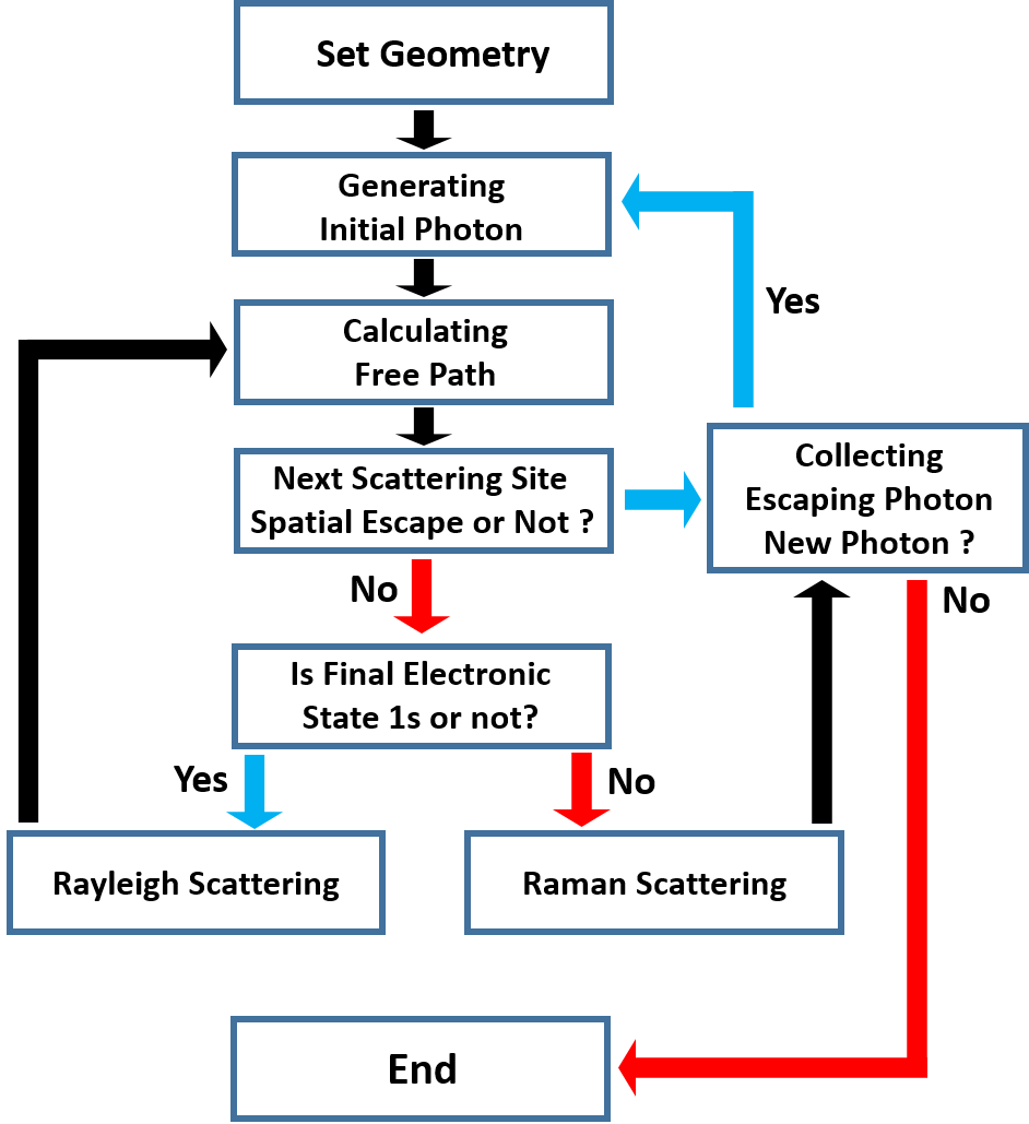
Fig. 2 shows a flow chart for radiative transfer simulations using STaRS. A simulation starts with the setup of the scattering geometry by assigning to each cell appropriate physical conditions. Initial far UV photons are generated in accordance with our prescription of . Each photon is tagged with the information of the unit wavevector , the position vector , the wavelength , and the density matrix composed of the Stokes parameters, , , , and . The free path for next scattering position is computed by transforming the scattering optical depth into the physical depth.
Decision is made whether the photon escapes from the region or is scattered into another direction. If the next scattering position is outside the scattering region, the photon is assumed to reach the observer as a far UV photon. Otherwise, we generate a new photon using the scattering phase function for an electric dipole process and determine the scattering type. We assume that the region is transparent to Raman-scattered photons. The scattered photon escapes from the scattering region if the scattering is Raman. Otherwise, the Rayleigh scattered photon is regarded as an incident photon propagating to a new scattering position. The procedure is repeated until escape.
In Sec. 2.1 and 2.2, we provide more detailed descriptions on the scattering geometry and generation of initial far UV photon prescribed by . In Sec. 2.3, we describe the computation of a free path . We discuss the basic properties of the scattered photons in Sec. 2.4.

2.1 Geometry : Scattering Region
The medium for radiative transfer through Raman and Rayleigh scattering corresponds to a thick H I region that is easily found in the slow stellar wind from a red giant (Lee & Lee 1997; Lee et al. 2019). No consideration on the thermal motion of neutral hydrogen is given because the variation of the cross section and the branching ratio in the scale of thermal speed is negligible (Chang et al. 2015; Chang et al. 2018).
In our simulation, we divide the scattering region into a large number of cells having a fixed size. Each cell is identified by a set of three indices with and running from 1 to and . If we denote by and the range of coordinates for the scattering region, the boundary of the th cell on the axis is given by
| (1) |
We also define and in a similar way.
Therefore, for any point in the cell identified with , we have
| (2) | |||
Each cell is also identified by its center point, whose coordinates are given by the following relations
| (3) | |||
2.2 Emission Source : Initial Photon
The operation of Raman scattering with atomic hydrogen requires the coexistence of a strong far UV source and a thick neutral region. In the case of symbiotic stars and young planetary nebulae, a strong far UV emission region is formed near an accreting white dwarf or a hot central star and a thick neutral region is also present in association with the mass loss of a giant star. In the simulation, the emissivity is prescribed as a function of wavelength and position. Regarding as the normalized probability density function, we pick a wavelength and a starting position of an initial photon in accordance with .
We find the spatial index from to determine the cell that contains the starting position. For simplicity, we assume that the initial photon is completely unpolarized and that the unit wavevector of the initial photon is selected from an isotropic distribution. Thus, the initial unit wavevector is obtained using two uniform random numbers and between 0 and 1 with the following prescription
| (4) | |||||
Because scattered radiation is polarized in an anisotropic geometry, it is important to carry the polarization information. The four Stokes parameters are necessary to describe the polarization state. An equivalent way is provided by considering the density matrix defined by
| (5) |
.
In our simulation, the Stokes parameter , representing circular polarization, is always set to zero because no circular polarization develops from initially unpolarizd photons in electric dipole processes associated with Raman and Rayleigh scattering. Initially unpolarized photons are described by a simple is given by
| (6) | |||||
The wavelength measured by an observer lying on the photon path is kept in the simulation. We assume that the emitters are in random motion and also subject to the bulk motion associated with the grid. If we let the velocity of the emitter be including bulk and random velocities, the wavelength in the grid frame is given by
| (7) |
where is the velocity of the cell .
2.3 Journey of Photon: Optical Depth and Free Path
The generation of an initial photon is followed by the estimate of the free optical depth given by
| (8) |
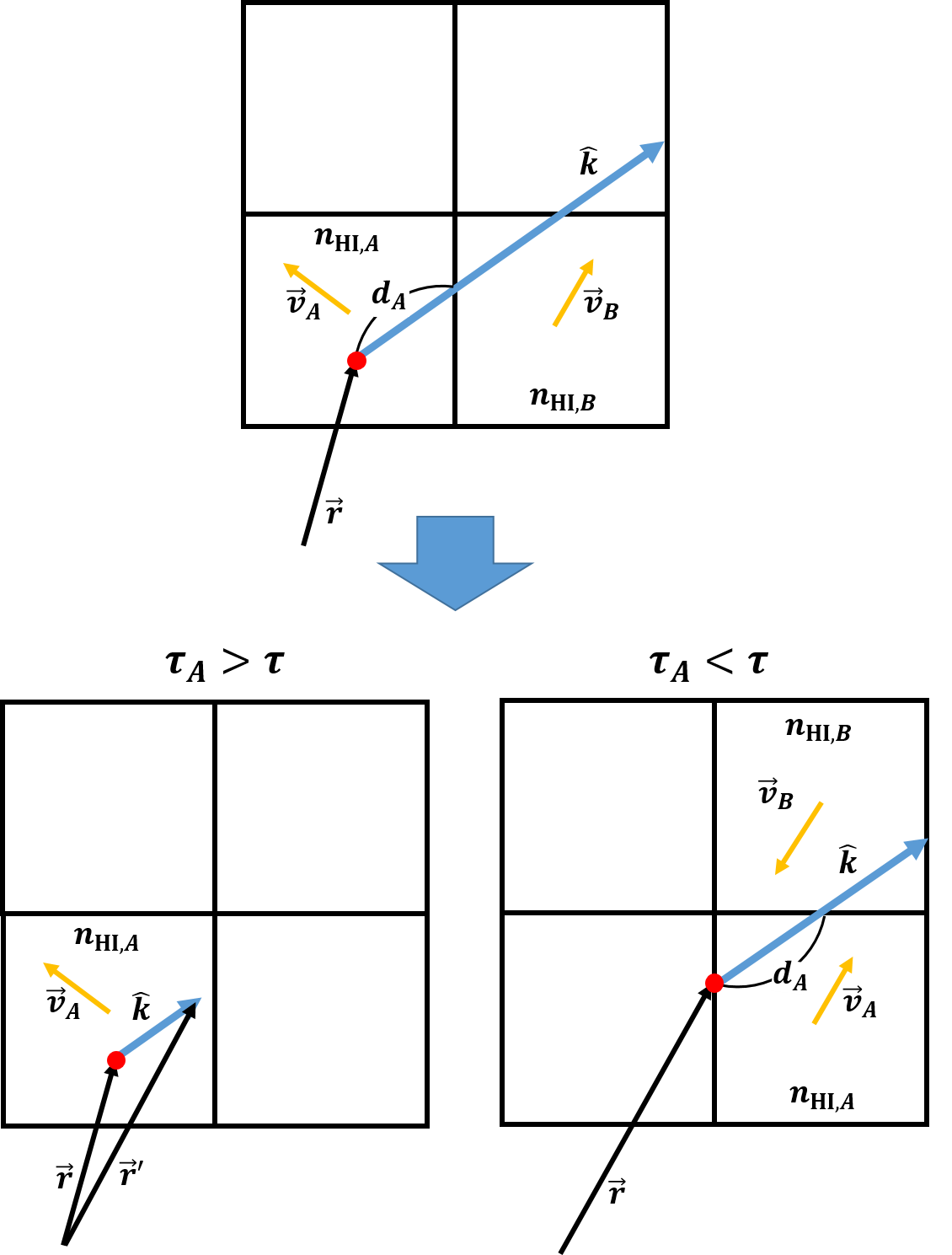
where is a uniform random number between and . We adopt the method in Seon 2009 to compute the free path and the next scattering position in grid-based geometry. In this section, we provide a brief description to compute the free path and determine the scattering position.
If the starting position of the photon is in cell , we measure the distance to the boundary of the cell along the photon ray from the starting position. With we define the scattering optical depth to the cell boundary by
| (9) |
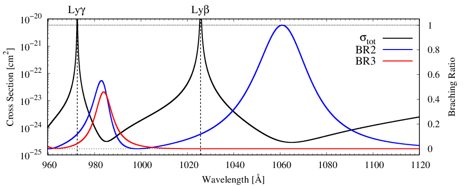
where is the wavelength in cell . Fig. 3 shows the total scattering cross section as a function of wavelength. If , then the next scattering position is found in cell as follows
| (10) |
In the opposite case where , the photon enters the neighboring cell . In this case, the same problem is obtained if we regard the entry point as the new starting point of the photon with a new free optical path reduced by , or
| (11) |
It should be noted that we are dealing with radiative transfer in a medium in motion. Therefore, cell may move with a velocity different from that of cell , in which case the photon wavelength along its propagation direction may change on entering cell from cell . Denoting by and the velocities of cells and , respectively, we have
| (12) |
Iterations from Eq. 9 are made with necessary updates , , and and new naming of cell as cell until we have . Fig. 4 shows a schematic illustration of this procedure. In cases when a neighboring cell may not exist and is outside the geometry, the photon is regarded as Rayleigh-escaped.
2.4 Rayleigh and Raman Scattering
Raman scattering with atomic hydrogen with the initial and final electronic states being and shares the same the scattering phase function with Rayleigh scattering with atomic hydrogen in (Chang et al. 2015, e.g.). It is also notable that the scattering is sufficiently far from resonance, the scattering phase function is the same as that of Thomson scattering. In this section, we describe the density matrix formalism with which the polarization and the unit wavevector of the scattered photon is determined (Ahn & Lee 2015; Chang et al. 2017). We also describe the wavelength conversion and the line broadening associated with Raman scattering.
According to the density matrix formalism, the probability density of the scattered wavevector is given by
| (13) |
where is defined by
| (14) |
Here, and are the polarization basis vector associated with and , respectively. Specifically, and so that represents polarization in the direction perpendicular to the plane spanned by the photon wavevector and the axis.
The components of the density matrix associated with the scattered radiation are related to those of incident radiation by
| (15) | |||||
where . In the code, a selection is made for from an isotropic distribution to compute . A new random deviate is compared with . If , then the selection of is accepted. Otherwise, the process is iterated until the acceptance is obtained. The scattered photon now becomes a new incident photon propagating to a new scattering site. This is followed by necessary updates for the wavevector and the density matrix given by
| (16) | |||||
The scattering type is determined by the branching ratio. If an incident far UV photon is more energetic than Ly, the final states available for Raman scattering include , and states. For photons near Ly, the total cross section is given by
| (17) |
where , , and are the scattering cross sections corresponding to the final states , , and , respectively. Rayleigh branching ratio is given by
| (18) |
In a similar way, Raman branching ratios corresponding to the final energy levels and are
| (19) |
In Fig. 3, the blue and red solid lines represent and , respectively.
The energy difference between the incident and Raman-scattered photons is the same as that between the initial and final atomic states. This is translated into the relation between the wavelengths and of the Raman-scattered and incident photons, respectively, which is given by
| (20) |
where is the wavelength corresponding to the energy difference between the initial and final states.
One very important aspect in Raman scattering can be found in the conspicuous change in line width. Differentiating Eq. (20), we have
| (21) |
from which we see immediately that the line width of Raman-scattered feature is broadened by the factor . For example, a typically observed line width of Raman-scattered O VI at 6825 Åamounts to Å whereas the far UV parent line O VI1032 exhibits a line width Å in many symbiotic stars.
Due to the line broadening effect, far UV radiation near Lyman series of hydrogen will be considerably diluted and redistributed around Balmer emission lines to appear as broad wings (Yoo et al. 2002; Chang et al. 2015; Chang et al. 2018, e.g.). Another important consequence of the line broadening effect is that the line profiles of Raman-scattered features mainly reflect the relative motion between the far UV emitters and the neutral scatterers and quite independent of the observer’s line of sight (Heo et al. 2016; Choi et al. 2020).
3 Code Test
As a check of our code, we present our simulation results for two exemplary cases. The first example is a static spherical H I region surrounding a far UV continuum source located at the center, in which Balmer wings are formed through Raman scattering. Analytic solutions are available for this case, against which our result obtained from STaRS is compared. The second case is reproduction of the result of Lee & Lee 1997, who investigated Raman scattering of O VI in symbiotic stars. In this case, the H I region is an expanding spherical wind around the giant component. Schematic illustrations of the two cases are shown in Fig. 5.
3.1 Formation of Balmer Wings in a Static Spherical H I Region
The central point-like far UV source surrounded by a spherical H I region with radius is characterized by a flat continuum. The static neutral region is assumed to be of uniform H I density . We fix the radial column density defined by
| (22) |
and vary the number of cells. We set , so that the total number of cells is given by . We generate photons for each simulation. The initial photons are generated at the center of the H I sphere in accordance with the emisivity given by the three dimensional Dirac delta function
| (23) |
where and are the maximum and minmum wavelengths of initial photons.
Fig. 6 shows optical spectra formed through Raman scattering for the cases of and 100. The vertical axis shows the Raman conversion efficiency () defined as the number ratio per unit wavelength of incident far UV photons and Raman-scattered optical photons. The left and right panels show Balmer wings formed through Raman scattering around H and H, respectively. The solid lines represent the analytic solutions and open circles show simulation results obtained using STaRS. The analytic solutions are obtained from the non-grid based simulation in Chang et al. 2015; Chang et al. 2018.
Far from the line centers, the simulation results for are slightly higher than the analytic solutions. Other than this, the agreement is fairly good, indicating little dependence on in the case of a static H I region. The volume of the H I region with is larger than the sphere with the radius as the H I density associated with a cell is determined by the central position of the cell. When is smaller than , the H I density of the cell is assigned to be . Otherwise, the density is assigned to be zero. The number ratio between Raman scattered photons near H and the total initial photons near Ly is 20.77 % for the analytic solution, whereas the simulations give 21.17, 20.91, and 20.77 % for , 10, and 100, respectively.
In Fig. 7, we present the polarimetric data of Raman scattered H projected to the celestial sphere. The surface brightness, the degree of polarization , and the direction of polarization are shown in the left, middle and the right panels, respectively. Here, in terms of the Stokes parameters, the degree of polarization and the position angle are given by
| (24) |
In the left panels, the surface brightness is shown in logarithmic scale. With our choice of a rather large value of , a considerable fraction of Raman-scattered photons are formed near the source, which leads to excellent agreement between the analytic results and those obtained using STaRS. One may notice increase in smoothness of the surface brightness as increases. It is also noticeable that becomes large with increasing distance from the center. The concentric polarization pattern reflects the spherically symmetric scattering geometry. In this particular case, appears to be sufficient to describe the the analytic result of the static medium.
3.2 Raman Scattering of O VI in Expanding H I Region
Lee & Lee 1997 presented their basic study of line formation of Raman O VI in a symbiotic star consisting of a white dwarf and a mass losing giant. The O VI emission region near the white dwarf component was assumed to be a point source broadened thermally with . For simplicity, the slow stellar wind from the red giant component is assumed to be entirely neutral ignoring the photoionization by the white dwarf. The orbital separation is of which is the radius of the red giant. The positions of the white dwarf and the red giant are and , respectively. The initial photons are generated at the position of the white dwarf according to the emissivity given by
| (25) | |||
where is the center wavelength of O VI 1032 and is the thermal width of O VI 1032 with .
The velocity and H I number density are the functions of the distance from the red giant are given by
| (26) | |||||
where is the characteristic number density defined in Eq. 2.11 of Lee & Lee 1997 and is the terminal velocity. As a second code test case, we revisit Raman O VI formation illustrated in Figs. 1 and 6 of Lee & Lee 1997. Fixing , we consider the three values of , 1, and 10, where . We generate photons for each simulation.
Fig. 8 shows the spectra and the Stokes parameter for Raman scattered O VI at 6825 Å. It should be noted that the integrated vanishes due to the axial symmetry about the axis. Therefore, the signed ratio represents the degree and direction of polarization, where a positive and a negative correspond to the polarization in direction perpendicular and parallel to the axis, respectively. The observer’s line of sight lies in - plane. Noting that it is perpendicular to the symmetry axis, maxium polarization can be developed along this direction or the symmetry axis. We collecte the photons escaping toward the observer. The fraction of the collected Raman photons near 6825 Å is 0.11, 0.21, and 1.82 % for , 1, and 10, respectively.
The line profiles obtained using STaRS differ slightly from those Lee & Lee 1997 presented. In particular, the red peaks obtained from STaRS are more enhanced than those presented by Lee & Lee 1997, which is attributed to the geometrical truncation adopted by them. The difference is in the range of 10-15 per cent with respect to the red peak. We find that the agreement gets better where the full range of the scattering region is taken into account. In the bottom panels, we find overall agreement in the polarization behaviors. The noisy features with are attributed to the small number statistics of collected photons. Blue photons are scattered mostly in the compact and dense region between the red giant and white dwarf, resulting in development of strong polarization in the direction perpendicular to the axis. In contrast, red photons are scattered mainly in a quite extended region near the red giant, leading to weak polarization and enhanced line flux.
Fair agreement shown in Fig. 6 and 8 demonstrates that STaRS has been well-tested. Furthermore, as illustrated in Fig. 7, STaRS is capable of study of radiative transfer for spectropolarimetric imaging observations.


4 Summary
We have developed a 3D grid-based Monte Carlo code ’STaRS’ for radiative transfer through Raman and Rayleigh scattering, which can be mainly used to investigate line formation of Raman-scattered features in a thick neutral region illuminated by a strong far UV emission source. Favorable conditions for Raman scattering with atomic hydrogen are easily met in symbiotic stars, young planetary nebulae and active galactic nuclei. Through a couple of tests, we have successfully demonstrated that ’STaRS’ is a flexible code to deal with radiative transfer in a thick neutral media yielding multidimensional spectropolarimetric and imaging data. ’STaRS’ is easily accessed in Github ’https://github.com/csj607/STaRS’.
Acknowledgements.
This research was supported by the Korea Astronomy and Space Science Institute under the R&D program (Project No. 2018-1-860-00) super-vised by the Ministry of Science, ICT and Future Planning. This work was also supported by a National Research Foundation of Korea (NRF) grant funded by the Korea government (MSIT; No. NRF-2018R1D1A1B07043944). Seok-Jun is very grateful to Dr. Kwang-Il Seon for his help in adoption of grid-based technique.References
- Ahn & Lee (2015) Ahn, S.-H., Lee, H.-W., 2015, Polarization of Lyman Emergent from a Thick Slab of Neutral Hydrogen, JKAS, 48, 195
- Akras et al. (2019) Akras, S., Guzman-Ramirez, L., Leal-Ferreira, M. L., Ramos-Larios, G., 2019, A Census of Symbiotic Stars in the 2MASS, WISE, and Gaia Surveys, ApJS, 240, 21
- Angel (1969) Angel, J. R. P., 1969, Polarization of Thermal X-Ray Sources, ApJ, 158, 219
- Arrieta & Torres-Peimbert (2002) Arrieta, A., Torres-Peimbert, S., 2002, Broad H Wings in Young Planetary Nebulae RMxAC, 12, 154
- Bethe & Salpeter (1967) Bethe, H. A., Salpeter, E. E., 1967, Quantum Mechanics of One and Two Electron Atoms, Academic Press, New York
- Brinch & Hogerheijde (2010) Brinch, C., Hogerheijde, M. R., 2010, LIME – a flexible, non-LTE line excitation and radiation transfer method for millimeter and far-infrared wavelengths, A&A, 523, A25
- Birriel (2004) Birriel, J. J., 2004, Raman-scattered He II at 4851 Åin the symbiotic stars HM Sagittae and V1016 Cygni, ApJ, 612, 1136
- Celnikier & Lefévre (1974) Celnikier, L. M., Lefévre, J., 1974, Radiation transport in circumstellar dust – A Monte Carlo approach, A&A, 36, 429
- Chang et al. (2015) Chang, S.-J., Heo, J.-E., Di Mille, F., Angeloni, R., Palma, T., Lee, H.-W., 2015, Formation of Raman scattering wings around H, H, and Pa in active galactic nuclei, ApJ, 814, 98
- Chang et al. (2017) Chang, S.-J., Lee, H.-W., Yang, Y., Polarization of Rayleigh scattered Ly in active galactic nuclei, 2017, MNRAS, 464, 5018
- Chang et al. (2018) Chang, S.-J., Lee, H.-W., Lee, H.-G., Hwang, N., Ahn, S.-H., Park, B.-G., 2018, Broad Wings around H and H in the Two S-type Symbiotic Stars Z Andromedae and AG Draconis, ApJ, 866, 129
- Chen et al. (2017) Chen, Z., Frank, A., Blackman, E. G., Nordhaus, J., Carroll-Nellenback, J., 2017, Mass transfer and disc formation in AGB binary systems, MNRAS, 468, 4465
- Choi et al. (2020) Choi, B.-E., Chang, S.-J., Lee, H.-G., Lee, H.-W., 2020, Line Formation of Raman-scattered He II 4851 in an Expanding Spherical H I Shell in Young Planetary Nebulae, ApJ, 889, 2
- Choi & Lee (2020) Choi, B.-E., Lee, H.-W., 2020, Discovery of Raman-scattered He II 6545 in the Planetary Nebulae NGC 6886 and NGC 6881, ApJL, 903L, 39
- de Val-Borro et al. (2017) de Val-Borro, M., Karovska, M., Sasselov, D. D., Stone, J. M., 2017, Three-dimensional hydrodynamical models of wind and outburst-related accretion in symbiotic systems, MNRAS, 468, 3408
- Dopita et al. (2016) Dopita, M. A., Nicholls, D. C., Sutherland, R. S., Kewley, L. J., Groves, B. A., 2016, The discovery of Raman scattering in H II regions, ApJL, 824, L13
- Eide et al. (2018) Eide, M. B., Gronke, M., Dijkstra, M., Hayes, M., 2018, ApJ, Unlocking the Full Potential of Extragalactic Ly through Its Polarization Properties, 856, 156
- Groves et al. (2002) Groves, B., Dopita, M. A., Williams, R. E., Hua, C.-T., 2002, The internal extinction curve of NGC 6302 and its extraordinary spectrum, PASA, 19, 425
- Harries & Howarth (1996) Harries, T. J., Howarth, I. D., 1996, Raman scattering in symbiotic stars. I. Spectropolarimetric observations, A&AS, 119, 61
- Heo & Lee (2015) Heo, J.-E., Lee, H.-W., 2015, Accretion flow and disparate profiles of Raman scattered O VI 1032, 1038 in the symbitic star V1016 Cygni, JKAS, 48, 105
- Heo et al. (2016) Heo, J.-E., Angeloni, R., Di Mille, F., Palma, T., Lee, H.-W., 2016, A Profile Analysis of Raman-scattered O VI Bands at 6825 Å and 7082 Å in Sanduleak’s Star, ApJ, 833, 286
- Jung & Lee (2004) Jung, Y.-C., Lee, H.-W., 2004, Centre shift of the Raman scattered He II 4850 in the symbiotic star V1016 Cygni, MNRAS, 355, 221
- Kang et al. (2009) Kang, E.-H., Lee, B.-C., Lee, H.-W., 2009, Raman-Scattered He II 6545 in the Young and Compact Planetary Nebula NGC 6790, ApJ, 695, 542
- Lee & Park (1999) Lee, H.-W., Park. M.-G., 1999, Toward the Evidence of the Accretion Disk Emission in the Symbiotic Star RR Telescopii, ApJL, 515, L89
- Lee (2000) Lee, H.-W., 2000, Raman-Scattering Wings of H in Symbiotic Stars, ApJ, 541, 25
- Lee et al (2001) Lee, H.-W., Kang, Y.-W., Byun, Y.-I., 2001, Raman-scattered He II Line in the Planetary Nebula M2-9 and in the Symbiotic Stars RR Telescopii and He 2-106, ApJ, 551, 121
- Lee et al. (2006) Lee, H.-W., Jung, Y.-C., Song, I.-O., Ahn, S.-H., 2006, Raman-scattered He II 4850, 6545 in the Young and Compact Planetary Nebula IC 5117, ApJ, 636, 1045
- Lee & Lee (1997) Lee, K.-W., Lee, H.-W., 1997, On the profiles and the polarization of Raman-scattered emission lines in symbiotic stars – II. Numerical simulations, MNRAS, 292, 573
- Lee et al. (2019) Lee, Y.-M., Lee, H.-W., Lee, H.-G., Angeloni, R., 2019, Stellar-wind accretion and Raman-scattered O VI features in the symbiotic star AG Draconis, MNRAS, 487, 2166
- Miller & Goodrich (1990) Miller, J. S., Goodrich, R. W., 1990, Spectropolarimetry of high-polarization Seyfert 2 galaxies and unified Seyfert theories, ApJ, 355, 456
- Nussbaumer et al. (1989) Nussbaumer, H., Schmid, H. M., Vegel, M., 1989, Raman scattering as a diagnostic possibility in astrophysics, A&A, 211L, 27
- Pequignot el al. (1997) Pequignot, D., Baluteau, J.-P., Morisset, C., Boisson, C., 1997, NGC7027: Discovery of a Raman line in a planetary nebula, A&A, 323, 217
- Saladino et al. (2018) Saladino, M. I., Pols, O. R., van der Helm, E., Pelupessy, I., Portegies Zwart, S., 2018, Gone with the wind: the impact of wind mass transfer on the orbital evolution of AGB binary systems, A&A, 618, A50
- Saslow & Mills (1969) Saslow, W. M., Mills, D. L., 1969, Raman scattering by hydrogenic systems, Phys. Rev., 187, 1025
- Sakurai (1967) Sakurai, J. J., 1967, Advanced Quantum Mechanics, Addison-Wesley, Reading, MA.
- Schild & Schmid (1996) Schild, H., Schmid, H. M., 1996, Spectropolarimetry of symbiotic stars. On the binary orbit and the geometric structure of V1016 Cygni, A&A, 310, 211
- Schmid (1989) Schmid, H. M., 1989, Identification of the emission bands at 6830, 7088 Å, A&A, 211L, 31
- Schmid (1992) Schmid, H. M., 1992, Monte-Carlo simulations of Raman scattered O VI emission lines in symbiotic stars, A&A, 254, 224
- Schmid (1995) Schmid, H. M., 1995, Monte Carlo simulations of the Rayleigh scattering effects in symbiotic stars, MNRAS, 275, 227
- Seon et al. (1994) Seon, K.-I., Min, K. W., Choi, C. S., Nam, U. W., 1994, Monte Carlo simulation of comptonization in a spherical shell geometry, JKAS, 27, 45
- Seon (2009) Seon, K.-I., 2009, Monte-Carlo Simulation of the Dust Scattering, PKAS, 24, 43
- Seon (2015) Seon, K.-I., 2015, Monte-Carlo Radiative Transfer Model of the Diffuse Galactic Light, JKAS, 47, 57
- Seon & Kim (2020) Seon, K.-I., Kim, C.-G., 2020, Ly-alpha Radiative Transfer: Monte-Carlo Simulation of the Wouthuysen-Field Effect, ApJS, 250, 9
- Sekeráš & Skopal (2015) Sekeráš, M., Skopal, A., 2015, Mass-loss Rate by the Mira in the Symbiotic Binary V1016 Cygni from Raman Scattering, ApJ, 812, 162
- Shore et al. (2010) Shore, S. N., Wahlgren, G. M., Genovali1, K., Bernabei, S., Koubsky, P., 2010, The spectroscopic evolution of the symbiotic star AG Draconis: I. The O VI Raman, Balmer, and helium emission line variations during the outburst of 2006-2008, A&A, 510, A70
- Storey & Hummer (1995) Storey, P. J., Hummer, D. G., 1995, Recombination line intensities for hydrogenic ions – IV. Total recombination coefficients and machine-readable tables for to 8, MNRAS, 272, 41
- Tran (2010) Tran, H. D., 2010, Hidden Double-peaked Emitters in Seyfert 2 Galaxies, ApJ, 711, 1174
- van Groningen (1993) van Gronigen, E., 1993, Further evidence for Raman scattering in RR Tel, MNRAS, 264, 975
- Yoo et al. (2002) Yoo, J. J., Bak, J.-Y., Lee, H.-W., 2002, Polarization of the broad H wing in symbiotic stars, MNRAS, 336, 467