Towards Generalized Implementation of
Wasserstein Distance in GANs
Abstract
Wasserstein GANs (WGANs), built upon the Kantorovich-Rubinstein (KR) duality of Wasserstein distance, is one of the most theoretically sound GAN models. However, in practice it does not always outperform other variants of GANs. This is mostly due to the imperfect implementation of the Lipschitz condition required by the KR duality. Extensive work has been done in the community with different implementations of the Lipschitz constraint, which, however, is still hard to satisfy the restriction perfectly in practice. In this paper, we argue that the strong Lipschitz constraint might be unnecessary for optimization. Instead, we take a step back and try to relax the Lipschitz constraint. Theoretically, we first demonstrate a more general dual form of the Wasserstein distance called the Sobolev duality, which relaxes the Lipschitz constraint but still maintains the favorable gradient property of the Wasserstein distance. Moreover, we show that the KR duality is actually a special case of the Sobolev duality. Based on the relaxed duality, we further propose a generalized WGAN training scheme named Sobolev Wasserstein GAN (SWGAN), and empirically demonstrate the improvement of SWGAN over existing methods with extensive experiments.11 1 Code is available at https://github.com/MinkaiXu/SobolevWassersteinGAN.
1 Introduction
Generative adversarial networks (GANs) [13] have attracted huge interest in both academia and industry communities due to its effectiveness in a variety of applications. Despite its effectiveness in various tasks, a common challenge for GANs is the training instability [14]. In literature, many works have been developed to mitigate this problem [3, 23, 17, 25, 26, 39].
By far, it is well known that the problem of training instability of the original GANs mainly comes from the ill-behaving distance metric [3], i.e., the Jensen-Shannon divergence metric, which remains constant when two distributions are disjoint. The Wasserstein GAN [4] improves this by using the Wasserstein distance, which is able to continuously measure the distance between two distributions. Such a new objective has been shown to be effective in improving training stability.
In practice, since the primal form of the Wasserstein distance is difficult to optimize, the WGAN model [4] instead proposed to optimize it with the Kantorovich-Rubinstein (KR) duality [37]. However, though the new WGAN scheme is theoretically more principled, it does not yield better performance in practice compared to other variants of GANs [23]. The main obstacle is that the WGAN requires the discriminator (or the critic) to be a Lipschitz function. However, this is very hard to satisfy in practice though a variety of different implementations have been tried such as weight clipping [4], gradient penalty (GP) [15], Lipschitz penalty (LP) [34] and spectral normalization (SN) [28]. As a result, WGAN is still unable to always achieve very compelling results.
In this paper, we argue that the strong Lipschitz condition might be unnecessary in the inner optimization loop for WGAN’s critic. Intuitively, a looser constraint on the critic, which results in a larger function space, can simplify the practical constrained optimization problem of the restricted critic, and the better-trained critic would further benefit the training of the generator. Therefore, instead of developing new methods to impose the Lipschitz constraint, in this paper we propose to relax this constraint. In other words, we move our attention from “how to better implement the Lipschitz constraint” to “how to loosen the Lipschitz constraint”. More specifically, in this paper we demonstrate a new dual form of the Wasserstein distance where the Lipschitz constraint is relaxed to the Sobolev constraint [1, 30]. We further show that the new duality with the relaxed constraint indeed is a generalization of the KR duality, and it still keeps the gradient property of the Wasserstein distance. Based on this relaxed duality, we propose a generalized WGAN model called Sobolev Wasserstein GAN. To the best of our knowledge, among the restricted GAN models [4, 15, 30, 29, 7, 2], Sobolev Wasserstein GAN is the most relaxed one that can still avoid the training instability problem.
The main contributions of this paper can be summarized as follows:
- •
We demonstrate the Sobolev duality of Wasserstein distance and demonstrate that the new duality is also capable of alleviating the training instability problem in GANs (Section 3.1). We further clarify the relation between Sobolev duality and other previous metrics and highlight that by far Sobolev duality is the most relaxed metric that can still avoid the non-convergence problem in GANs (Section 3.2).
- •
We conduct extensive experiments to study the practical performance of SWGAN. We find that generally our proposed model achieves better sample quality and is less sensitive to the hyper-parameters. We also present a theoretical analysis of the minor sub-optimal equilibrium problem common in WGAN family models, and further propose an improved SWGAN with a better convergence.
2 Preliminaries
2.1 Generative adversarial networks
Generative adversarial networks [13] perform generative modeling via two competing networks. The generator network learns to map samples from a noise distribution to a target distribution, while the discriminator network is trained to distinguish between the real data and the generated samples. Then the generator is trained to output images that can fool the discriminator . The process is iterated. Formally, the game between the generator and the discriminator leads to the minimax objective:
| (1) |
where denotes the distribution of real data and denotes the noise distribution.
This objective function is proven to be equivalent to the Jensen-Shannon divergence (JSD) between the real data distribution and fake data distribution when the discriminator is optimal. Assuming the discriminator is perfectly trained, the optimal discriminator is as follows:
| (2) |
However, recently [42] points out that the gradients provided by the optimal discriminator in vanilla GAN cannot consistently provide meaningful information for the generator’s update, which leads to the notorious training problems in GANs such as gradient vanishing [13, 3] and mode collapse [9, 27, 21, 6]. This view would be clear when checking the gradient of optimal discriminator in Eq. (2): the value of the optimal discriminative function at each point is independent of other points and only reflects the local densities of and , thus, when the supports of the two distributions are disjoint, the gradient produced by a well-trained discriminator is uninformative to guide the generator [42].
2.2 Wasserstein distance
Let and be two data distributions on . The Wasserstein- distance between and is defined as
| (3) |
where the coupling of and is the probability distribution on with marginals and , and denotes the set of all joint distributions . The Wasserstein distance can be interpreted as the minimum cost of transporting one probability distribution to another. The Kantorovich-Rubinstein (KR) duality [37] provides a new way to evaluate the Wasserstein distance between distributions. The duality states that
| (4) | ||||
where the supremum is taken over all functions : whose Lipschitz constant is no more than one.
2.3 Wasserstein GAN
The training instability issues of vanilla GAN is considered to be caused by the unfavorable property of distance metric [3], i.e., the JSD remains constant when the two distributions are disjoint. Accordingly, [4] proposed Wasserstein distance in the form of KR duality Eq. (4) as an alternative objective.
The Wasserstein distance requires to enforce the Lipschitz condition on the critic network . It has been observed in previous work that imposing Lipschitz constraint in the critic leads to improved stability and sample quality [4, 21, 12, 11]. Besides, some researchers also found that applying Lipschitz continuity condition to the generator can benefit the quality of generated samples [40, 33]. Formally, in WGAN family, with the objective being Wasserstein distance, the optimal critic under Lipschitz constraint holds the following property [15]:
Proposition 1.
This property indicates that for each coupling of generated datapoint and real datapoint in , the gradient at any linear interpolation between and is pointing towards the real datapoint with unit norm. Therefore, guided by the gradients, the generated sample would move toward the real sample . This property provides the explanation, from the gradient perspective, on why WGAN can overcome the training instability issue.
2.4 Sobolev space
Let be a compact space in and let (x) to be a distribution defined on as a dominant measure. Functions in the Sobolev space [1] can be written as:
| (5) |
Restrict functions to the Sobolev space vanishing at the boundary and denote this space by , then the semi-norm in can be defined as:
| (6) |
Given the notion of semi-norm, we can define the Sobolev unit ball constraint as follows:
| (7) | ||||
Sobolev unit ball is a function class that restricts the square root of integral of squared gradient norms according to the dominant measure .
2.5 Sobolev GAN
After WGAN, many works are devoted to improving GAN model by imposing restrictions on the critic function. Typical instances are the GANs based on Integral Probability Metric (IPM) [29, 7]. Among them, Sobolev GAN (SGAN) [30] proposed using Sobolev IPM as the metric for training GANs, which restricts the critic network in :
| (8) |
The following choices of measure for are considered, which we will take as our baselines:
- (a)
: the mixed distribution of and ;
- (b)
: , where , and , i.e., the distribution defined by the interpolation lines between and as in [15].
Let and be the cumulative distribution functions (CDF) of and respectively, and assume that the partial derivatives of and exist and are continuous. Define the differential operator where = , which computes high-order partial derivative excluding the -th dimension. Let . According to [30], the Sobolev IPM in Eq. (8) has the following equivalent form:
| (9) |
Note that, for each , is the cumulative distribution of the variable given the other variables weighted by the density function of at , i.e.,
| (10) |
Thus, the Sobolev IPM can be seen as a comparison of coordinate-wise conditional CDFs. Furthermore, [30] also proves that the optimal critic in SGAN holds the following property:
| (11) |
3 Sobolev duality of Wasserstein distance
3.1 Sobolev duality
Let and be two points in . The linear interpolation between and can be written as with . Regarding as a random variable on the line between and , we can then define its probability distribution as , which we will later use as the dominant measure for Sobolev space. Formally, let be the random variable that follows the uniform distribution U. Then can be written as:
| (12) |
With the above defined notation, we propose our new dual form of Wasserstein distance as follows, which we call Sobolev duality22 2 We provide the proofs of Sobolev duality and Proposition 2 in Appendix.
| (13) | ||||
where denotes the Sobolev unit ball of
| (14) |
Note that the support of is the straight line between and . Thus is the square root of the path integral of squared gradient norms from to . In other words, the constraint is restricting the gradient integral on each line between and to be no more than 1.
Corresponding to Proposition 1 of KR duality, we highlight the following property of the proposed Sobolev duality:
Proposition 2.
That is, with Sobolev duality, the gradient direction for every fake datum is the same as WGAN. Hence, enforcing the Sobolev duality constraint on discriminator can be an effective alternative of the Lipschitz condition to guarantee a stable training for GAN model.
3.2 Relation to other metrics
Relation to KR duality in Eq. (4). As indicated by Proposition 2, the optimal critic of Sobolev duality actually holds the same gradient property as KR duality in Proposition 1. However, as clarified below, the constraint in Sobolev duality is indeed looser than KR duality, which would potentially benefit the optimization.
In the classic KR duality , is restricted under Lipschitz condition, i.e., the gradient norms of all points in the metric space are enforced to no more than . By contrast, in our Sobolev duality, we restrict the integral of squared gradient norms over each line between and . This implies that Lipschitz continuity is a sufficient condition of the constraint in Sobolev duality. In summary, Sobolev duality is a generalization of KR duality where the constraint is relaxed, while still keeps the same property of training stability.
Relation to Sobolev IPM in Eq. (8). We now clarify the difference between Sobolev IPM in Eq. (8) and Sobolev duality of Wasserstein distance in Eq. (13). In the former metric, when implementing (defined in Section 2.5), the total integral of squared gradient norms on all interpolation lines between and is enforced to no more than ; while in the latter metric, the integral over each interpolation line between and is restricted. Therefore, Sobolev duality enforces stronger constraint than Sobolev IPM.
However, we should also note that the stronger constraint is necessary to ensure the favorable gradient property in Proposition 2. By contrast, as shown in Eq. (11), Sobolev IPM measures coordinate-wise conditional CDF, which cannot always provide gradients as good as the optimal transport plan in Wasserstein distance. A toy example is provided in Appendix to show the case that Sobolev IPM is sometimes insufficiently constrained to ensure the convergence.
4 Sobolev Wasserstein GAN
Now we define the GAN model with Sobolev duality, which we name as Sobolev Wasserstein GAN (SWGAN). Formally, SWGAN can be written as:
| (15) |
with the constraint that
| (16) |
where is the interpolation distribution on lines between pairs of points and as defined in Eq. (12).
Let denote , then the constraint is to restrict to be greater than or equal to 0 for all the pairs of . Inspired by [30], we define the following Augmented Lagrangian inequality regularization [32] corresponding to SWGAN ball constraints:
| (17) | ||||
where is the Lagrange multiplier, is the quadratic penalty weight and represents the slack variables. Practically, is directly substituted by its optimal solution:
| (18) |
As in [4] and [30], the regularization term in Eq. (17) is added to the loss only when training the critic. To be more specific, the training process is: given the generator parameters , we train the discriminator by maximizing ; then given the discriminator parameters , we train the generator via minimizing . We leave the detailed training procedure in Appendix.
5 Experiments
We tested SWGAN on both synthetic density modeling and real-world image generation task.
5.1 Synthetic density modeling
1D distribution modeling. Displaying the level sets is a standard qualitative approach to evaluate the learned critic function for two-dimensional data sets [15, 20, 34]. Here, we consider both real data distribution and generated fake distribution are fixed simple one-dimensional Gaussian distributions. Our goal is to investigate whether the critics of both WGAN and SWGAN can be efficiently optimized to provide the favorable gradients presented in Proposition 1 and 2. We observed that while both critics can be trained to the theoretical optimum, the latter one can always enjoy a faster convergence compared with the former one. An empirical example is visualized in Fig. 1. As shown here, with the same initial states and hyper-parameters, the critic of SWGAN holds a faster and smoother convergence towards the optimal state. This meaningful observation verifies our conjecture that a larger function space of the critic would benefit the training.
Level sets of the critic In this section we give another 2D level sets visualization. As analyzed in Section 3.1, Sobolev constraint in SWGAN is a generalization of Lipschitz constraint. Therefore, theoretically SWGAN critic should also be capable of modeling more challenging real and fake data and providing meaningful gradients. To demonstrate this, we train SWGAN critics to optimality on several toy distributions. The value surfaces of the critics are plotted in Figure 2, which shows good fitness of the distribution following our theoretical analysis.
5.2 Real-world image generation
5.2.1 Experimental setup
[b] GANs CIFAR-10 Tiny-ImageNet IS FID IS FID WGAN-GP∗ 7.85.07 18.21.12 8.17.03 18.70.05 WGAN-GP with 7.88.09 18.08.22 8.17.04 18.69.10 WGAN-AL 7.79.09 17.86.16 8.26.03 18.70.06 WGAN-AL with 7.89.09 17.52.27 8.31.02 18.61.09 SGAN∗, 7.81.11 17.89.27 8.30.04 18.90.04 SGAN∗, 7.83.10 18.03.24 8.31.03 18.90.08 SGAN, with 7.86.09 17.74.24 8.33.03 18.75.07 SWGAN-GP 7.98.08 17.50.19 8.38.03 18.50.03 SWGAN-AL 7.93.09 16.75.24 8.41.03 18.32.05
- *
denotes the vanilla version of our baselines.
Controlled variables. To make the comparisons more convincing, we also include extended versions of the existing GAN models to control the contrastive variables. The controlled variables includes:
- •
- •
Optimization method. In our baseline WGAN-GP [15], the restriction is imposed by Penalty Method (PM). By contrast, SGAN and SWGAN-AL use Augmented Lagrangian Method (ALM). ALM is a more advanced algorithm than PM for strictly imposing the constraint. To see the practical difference, we add experiment settings of SWGAN with penalty regularization term (named SWGAN-GP). Formally, the penalty can be written as:
(19) where is the gradient penalty coefficient. is the alternative term of the ALM penalty in Eq. (17) for the training of SWGAN-GP.
Baselines. For comparison, we also evaluated the WGAN-GP [15] and Sobolev GAN (SGAN) [30] with different sampling sizes and penalty methods. The choice of baselines is due to their close relation to SWGAN as analyzed in Section 3.2. We omit other previous methods since as a representative of state-of-the-art GAN model, WGAN-GP has been shown to rival or outperform a number of former methods, such as the original GAN [13], Energy-based generative adversarial network [41], the original WGAN with weight clipping [4], Least Squares GAN [24], Boundary equilibrium GAN [8] and GAN with denoising feature matching [38].
Evaluation metrics. Since GAN lacks the capacity to perform reliable likelihood estimations [36], we instead concentrate on evaluating the quality of generated images. We choose to compare the maximal Frechet Inception Distances (FID) [18] and Inception Scores [35] reached during training iterations, both computed from 50K samples. A high image quality corresponds to high Inception and low FID scores. Specifally, IS is defined as , where is the distribution of label conditioned on generated data , and is the marginal distribution. IS combines both the confidence of the class predictions for each synthetic images (quality) and the integral of the marginal probability of the predicted classes (diversity). The classification probabilities were estimated by the Inception model [35], a classifier pre-trained upon the ImageNet dataset [10]. However, in practice we note that IS is hard to detect the mode collapse problems. FID use the same Inception model to capture computer-vision-specific features of a collection of real and generated images, and then calculate the Frechet distance (also called - distance) [5] between two activation distributions. The intuition of IS is that high-quality images should lead to high confidence in classification, while FID is aiming to measure the computer-vision-specific similarity of generated images to real ones through Frechet distance (a.k.a., Wasserstein- distance) [5].
Data. We test different GANs on CIFAR-10 [22] and Tiny-ImageNet [10] , which are standard datasets widely used in GANs literatures. Both datasets consist of tens of thousands of real-world color images with class labels.
Network architecture. For all experimental settings, we follow WGAN-GP [15] and adopt the same Residual Network (ResNet) [16] structures and hyperparameters. Details of the architecture are provided in Appendix.
Other implementation details. For SWGAN metaparameter, we choose as the sample size . Adam optimizer [19] is set with learning rate decaying from to over 100K iterations with . We used critic updates per generator update, and the batch size used was .


5.2.2 Results
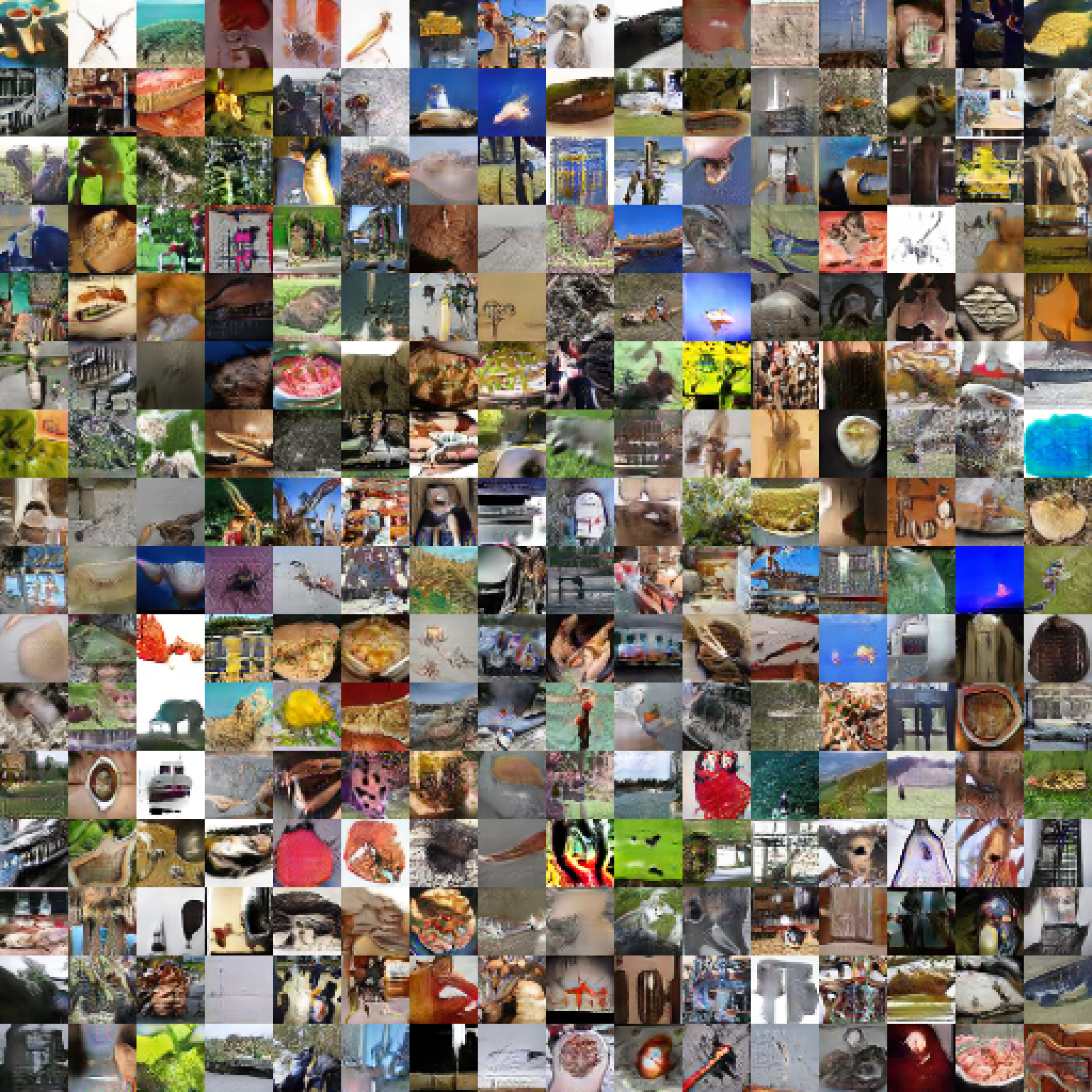
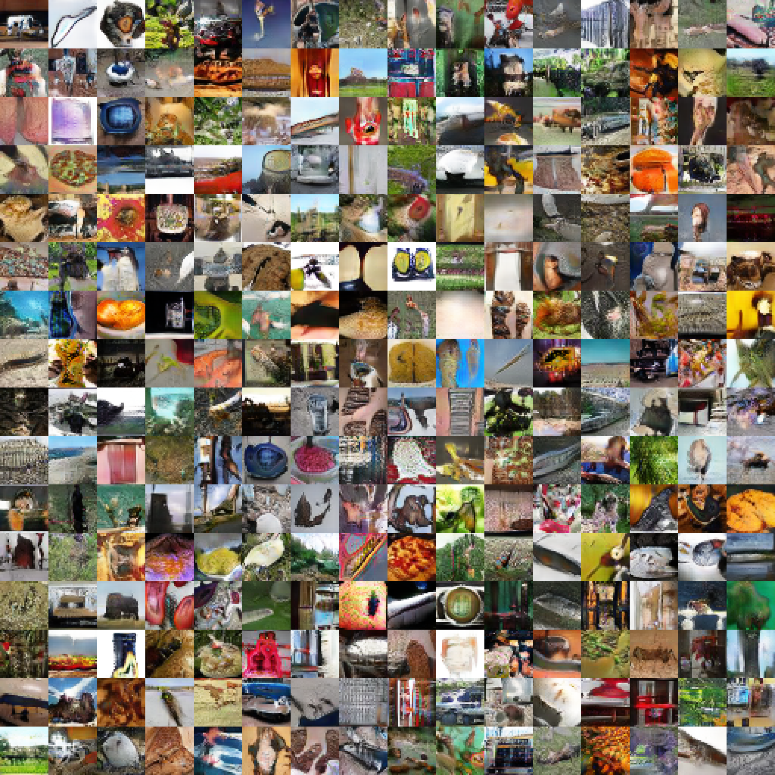
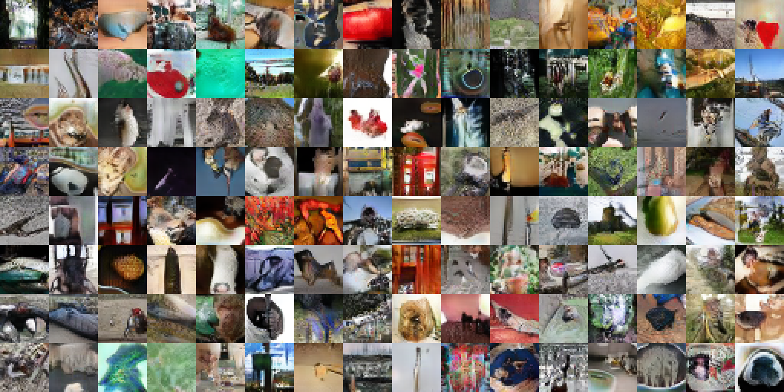
We here also introduce WGAN with Augmented Lagrangian Method (WGAN-AL) for further comparison, which is similar to SGAN [30]. Scores in terms of FID and IS on CIFAR-10 and Tiny-ImageNet are reported in Table 1. Some representative samples from the resulting generator of SWGAN are provided in Fig. 4 and Fig. 4. Some representative samples from the resulting generator of SWGAN are provided in Appendix. In experiments, we note that IS is remarkably unstable during training and among different initializations, while FID is fairly stable. So we plot the training curves in terms of FID on CIFAR-10 in Figure 6 to show the training process of different GANs.
From Table 1 and Figure 6, we can see that SWGANs generally work better than the baseline models. The experimental results also show that WGAN and SGAN tend to have slightly better performance when using ALM or sample more interpolation points. However, compared with SWGAN-AL and SWGAN-GP, the performances in these cases are still not competitive enough. This indicates that the larger sampling size and ALM optimization algorithm are not the key elements for the better performance of SWGAN, i.e., these results evidence that it is the relaxed constraint in Sobolev duality that leads to the improvement, which is in accordance with our motivation that a looser constraint would simplify the constrained optimization problem and lead to a stronger GAN model.
We further test SWGAN with different regularization terms and parameters on CIFAR-10. The scores are shown in Figure 6. As shown in Figure 6, generally ALM is a better choice when considering FID, while GP is better for IS. A meaningful observation is that SWGAN is not sensitive to different values of penalty weights and . By contrast, a previous large scale study reported that the performance of WGAN-GP holds strong dependence on the penalty weight (see Figure 8 and 9 in [23]). This phenomenon demonstrates a more smooth and stable convergence and well-behaved critic performance throughout the whole training process of SWGAN.
6 Local Convergence Analysis
Some literature pay attention to the sub-optimal convergence problem of GANs [25, 26, 6, 11], which is an important direction that deserves further investigation. Moreover, [26] recently shows that in some toy case that distributions that are not absolutely continuous, WGAN based models are not always convergent.
We employ the same prototypical counterexample to further analyze the convergence of SWGAN: the real data distribution is defined as a Dirac-distribution concentrated at 0; generator distribution is set as and the linear critic is set as . We also follow them to focus on investigating the gradient penalty version (SWGAN-GP). In the toy case, the regularizer term in Eq. (19) can be simplified to:
| (20) |
where is the gradient penalty target that set as in SWGAN-GP. Following the previous work, we set the object as and then study the sub-optimal convergence problem through the gradient vector field:
| (21) |
In practice, GANs are usually trained through either Simultaneous or Alternating Gradient Descent (SimGD and AltGD), which means updating the parameters according to the gradient field simultaneously or alternately. [26] proves that the unique equilibrium point in the above defined case is . However, in Eq. (21) the gradient field shows a discontinuity at the equilibrium point, which indicates that similar to WGAN-GP, SWGAN-GP also cannot converge locally in this case (Fig. 7(a), 7(b), and 7(c)). To bypass this minor sub-optimal problem, we design a zero-centered gradient penalty (SWGAN-CP) by simply setting the in Eq. (20) as and adding another penalty on the squared norm of the gradients (Fig. 7(d), 7(e), and 7(f)). The proof for the local convergence of SWGAN-CP is provided in Appendix.
However, as acknowledged by [26], despite these minor ill-behaviors, WGAN has been successfully applied in practice. Furthermore, in our real-world experiments, we also noticed that there are few positive improvements when taking zero-centered penalty as the regularization term.
7 Conclusion
In this paper, we proposed a new dual form of Wasserstein distance with the Lipschitz constraint relaxed and demonstrate that it is still capable of eliminating the training instability issues. This new dual form leads to a generalized WGAN model. We built Sobolev Wasserstein GAN based on the proposed duality and provided empirical evidence that our GAN model outperforms the previous approaches, which either impose the strong Lipschitz penalty or cannot theoretically guarantee the convergence.
This work was motivated by the intuition that with a less restricted function space, the critic would be easier to be trained to optimum, thus benefiting the training of GANs. To the best of our knowledge, Sobolev Wasserstein GAN is the GAN model with the most relaxed restriction that can still avoid the training instability problem. In the future, we hope that practitioners can take a step back and investigate whether we can further relax the constraint imposed on the function space of the critic and what the minimal requirement for the convergence guarantee could be.
References
- Adams and Fournier [2003] Robert A Adams and John JF Fournier. Sobolev spaces, volume 140. Elsevier, 2003.
- Adler and Lunz [2018] Jonas Adler and Sebastian Lunz. Banach wasserstein gan. In NIPS, 2018.
- Arjovsky and Bottou [2017] Martin Arjovsky and Léon Bottou. Towards principled methods for training generative adversarial networks. In ICLR, 2017.
- Arjovsky et al. [2017] Martin Arjovsky, Soumith Chintala, and Léon Bottou. Wasserstein generative adversarial networks. In ICML, 2017.
- Aronov et al. [2006] Boris Aronov, Sariel Har-Peled, Christian Knauer, Yusu Wang, and Carola Wenk. Fréchet distance for curves, revisited. In European Symposium on Algorithms. Springer, 2006.
- Arora et al. [2017] Sanjeev Arora, Rong Ge, Yingyu Liang, Tengyu Ma, and Yi Zhang. Generalization and equilibrium in generative adversarial nets (gans). arXiv preprint arXiv:1703.00573, 2017.
- Bellemare et al. [2017] Marc G Bellemare, Ivo Danihelka, Will Dabney, Shakir Mohamed, Balaji Lakshminarayanan, Stephan Hoyer, and Rémi Munos. The cramer distance as a solution to biased wasserstein gradients. arXiv preprint arXiv:1705.10743, 2017.
- Berthelot et al. [2017] David Berthelot, Thomas Schumm, and Luke Metz. Began: Boundary equilibrium generative adversarial networks. arXiv preprint arXiv:1703.10717, 2017.
- Che et al. [2016] Tong Che, Yanran Li, Athul Paul Jacob, Yoshua Bengio, and Wenjie Li. Mode regularized generative adversarial networks. arXiv preprint arXiv:1612.02136, 2016.
- Deng et al. [2009] Jia Deng, Wei Dong, Richard Socher, Li-Jia Li, Kai Li, and Li Fei-Fei. Imagenet: A large-scale hierarchical image database. In CVPR. Ieee, 2009.
- Farnia and Tse [2018] Farzan Farnia and David Tse. A convex duality framework for gans. In NIPS, 2018.
- Fedus et al. [2017] William Fedus, Mihaela Rosca, Balaji Lakshminarayanan, Andrew M Dai, Shakir Mohamed, and Ian Goodfellow. Many paths to equilibrium: Gans do not need to decrease a divergence at every step. arXiv preprint arXiv:1710.08446, 2017.
- Goodfellow et al. [2014] Ian Goodfellow, Jean Pouget-Abadie, Mehdi Mirza, Bing Xu, David Warde-Farley, Sherjil Ozair, Aaron Courville, and Yoshua Bengio. Generative adversarial nets. In NIPS, 2014.
- Goodfellow [2016] Ian Goodfellow. Nips 2016 tutorial: Generative adversarial networks. arXiv preprint arXiv:1701.00160, 2016.
- Gulrajani et al. [2017] Ishaan Gulrajani, Faruk Ahmed, Martin Arjovsky, Vincent Dumoulin, and Aaron C Courville. Improved training of wasserstein gans. In NIPS, 2017.
- He et al. [2016] Kaiming He, Xiangyu Zhang, Shaoqing Ren, and Jian Sun. Deep residual learning for image recognition. In CVPR, 2016.
- Heusel et al. [2017a] Martin Heusel, Hubert Ramsauer, Thomas Unterthiner, Bernhard Nessler, and Sepp Hochreiter. Gans trained by a two time-scale update rule converge to a local nash equilibrium. In NIPS, 2017.
- Heusel et al. [2017b] Martin Heusel, Hubert Ramsauer, Thomas Unterthiner, Bernhard Nessler, Günter Klambauer, and Sepp Hochreiter. Gans trained by a two time-scale update rule converge to a nash equilibrium. arXiv preprint arXiv:1706.08500, 2017.
- Kingma and Ba [2014] Diederik P Kingma and Jimmy Ba. Adam: A method for stochastic optimization. arXiv preprint arXiv:1412.6980, 2014.
- Kodali et al. [2017a] Naveen Kodali, Jacob Abernethy, James Hays, and Zsolt Kira. How to train your dragan. arXiv preprint arXiv:1705.07215, 2(4), 2017.
- Kodali et al. [2017b] Naveen Kodali, Jacob Abernethy, James Hays, and Zsolt Kira. On convergence and stability of gans. arXiv preprint arXiv:1705.07215, 2017.
- Krizhevsky et al. [2009] Alex Krizhevsky, Geoffrey Hinton, et al. Learning multiple layers of features from tiny images. Technical report, Citeseer, 2009.
- Lucic et al. [2017] Mario Lucic, Karol Kurach, Marcin Michalski, Sylvain Gelly, and Olivier Bousquet. Are gans created equal? a large-scale study. arXiv preprint arXiv:1711.10337, 2017.
- Mao et al. [2017] Xudong Mao, Qing Li, Haoran Xie, Raymond YK Lau, Zhen Wang, and Stephen Paul Smolley. Least squares generative adversarial networks. In CVPR, 2017.
- Mescheder et al. [2017] Lars Mescheder, Sebastian Nowozin, and Andreas Geiger. The numerics of gans. In NIPS, 2017.
- Mescheder et al. [2018] Lars Mescheder, Andreas Geiger, and Sebastian Nowozin. Which training methods for gans do actually converge? In ICML, 2018.
- Metz et al. [2016] Luke Metz, Ben Poole, David Pfau, and Jascha Sohl-Dickstein. Unrolled generative adversarial networks. arXiv preprint arXiv:1611.02163, 2016.
- Miyato et al. [2018] Takeru Miyato, Toshiki Kataoka, Masanori Koyama, and Yuichi Yoshida. Spectral normalization for generative adversarial networks. In ICLR, 2018.
- Mroueh and Sercu [2017] Youssef Mroueh and Tom Sercu. Fisher gan. In NIPS, 2017.
- Mroueh et al. [2018] Youssef Mroueh, Chun-Liang Li, Tom Sercu, Anant Raj, and Yu Cheng. Sobolev GAN. In ICLR, 2018.
- Nagarajan and Kolter [2017] Vaishnavh Nagarajan and J Zico Kolter. Gradient descent gan optimization is locally stable. In NIPS, 2017.
- Nocedal and Wright [2006] Jorge Nocedal and Stephen Wright. Numerical optimization. Springer Science & Business Media, 2006.
- Odena et al. [2018] Augustus Odena, Jacob Buckman, Catherine Olsson, Tom B Brown, Christopher Olah, Colin Raffel, and Ian Goodfellow. Is generator conditioning causally related to gan performance? arXiv preprint arXiv:1802.08768, 2018.
- Petzka et al. [2018] Henning Petzka, Asja Fischer, and Denis Lukovnikov. On the regularization of wasserstein GANs. In ICLR, 2018.
- Salimans et al. [2016] Tim Salimans, Ian Goodfellow, Wojciech Zaremba, Vicki Cheung, Alec Radford, and Xi Chen. Improved techniques for training gans. In NIPS, 2016.
- Theis et al. [2015] Lucas Theis, Aäron van den Oord, and Matthias Bethge. A note on the evaluation of generative models. arXiv preprint arXiv:1511.01844, 2015.
- Villani [2008] C. Villani. Optimal Transport: Old and New. Grundlehren der mathematischen Wissenschaften. Springer Berlin Heidelberg, 2008.
- Warde-Farley and Bengio [2016] David Warde-Farley and Yoshua Bengio. Improving generative adversarial networks with denoising feature matching. 2016.
- Yadav et al. [2017] Abhay Yadav, Sohil Shah, Zheng Xu, David Jacobs, and Tom Goldstein. Stabilizing adversarial nets with prediction methods. arXiv preprint arXiv:1705.07364, 2017.
- Zhang et al. [2018] Han Zhang, Ian Goodfellow, Dimitris Metaxas, and Augustus Odena. Self-attention generative adversarial networks. arXiv preprint arXiv:1805.08318, 2018.
- Zhao et al. [2016] Junbo Zhao, Michael Mathieu, and Yann LeCun. Energy-based generative adversarial network. arXiv preprint arXiv:1609.03126, 2016.
- Zhou et al. [2019] Zhiming Zhou, Jiadong Liang, Yuxuan Song, Lantao Yu, Hongwei Wang, Weinan Zhang, Yong Yu, and Zhihua Zhang. Lipschitz generative adversarial nets. In ICML, 2019.
Appendix A Algorithm for SWGAN-AL
Input: penalty weight, learning rate, number of critic iterations per generator iteration, batch size, number of points sampled between each pair of fake and real data
Initial: critic parameters , generator parameters , Lagrange multiplier
Appendix B Proofs for Sobolev duality
B.1 Proof of the Sobolev duality of Wasserstein Distance
We here provide a proof for our new dual form of Wasserstein distance.
The Wasserstein distance is given as follows
| (22) |
where denotes the set of all probability measures with marginals and on the first and second factors, respectively. The Kantorovich-Rubinstein (KR) dual is written as
| (23) | ||||
We will prove that Wasserstein distance in its dual form can also be written in Sobolev duality:
| (24) | ||||
where
| (25) |
which relaxes the Lipschitz constraint in the KR dual form of Wasserstein distance.
Theorem 1.
Given , we have .
Proof.
(i) As illustrated in Section 3.2.1, Lipschitz continuity is a sufficient condition of the constraint in Sobolev dual. Therefor, for any that satisfies “”, it must satisfy “”. Thus, .
(ii) Let a curve be the straight line from to with its tangent vector at some chosen point defined as , i.e., . Let be U and let be the random variable that follows . Let , which is a bijective parametrization of the curve such that and give the endpoints of . Given , we have:
| (26) | ||||
| (Directional derivative is less than norm of gradient) | ||||
| (27) | ||||
| (28) | ||||
| (Cauchy–Schwarz inequality) | ||||
| (29) | ||||
| (, see Eq. (14) in paper) | ||||
| (see Eq. (25) ) | ||||
| () |
Let .
Let and .
Let denote the complementary set of and define accordingly.
For , we have the following:
| (31) | ||||
.
(iii) Combining (i) and (ii), we have .
Given , we have . ∎
B.2 Proof of Proposition 1
Proposition 3.
Lemma 1.
Proof.
In addition, as illustrated in Section 3.2.1, 1-Lipschitz condition in Eq. (23) is the sufficient condition of Sobolev duality Eq. (24). Therefore, the function space of in KR duality Eq. (23) is a subspace of the function space defined in Sobolev duality Eq. (24).
(ii) Recently, [42] proposed another relaxed dual form of Wasserstein distance. It states that:
| (33) | ||||
It is worthy noticing that any under this constraint corresponds to one in Eq. (23) with the value of on and unchanged. Thus, any under the constraint in Eq. (33) also holds the property in Eq. (32).
According to Part (ii) of our proof in Section B.1, given the constraint in Sobolev duality Eq. (24), we can get the constraint in Eq. (33) that . Therefore, the restriction in Sobolev duality is the sufficient condition of Eq. (33), i.e., the function space of in Sobolev duality Eq. (24) is a subspace of the function space defined in Eq. (33).
(iii) Combining (i) and (ii), we have that
- •
- •
Therefore, we conclude that the optimal in Sobolev duality Eq. (24) also holds this property. ∎
Theorem 2.
If , given , then for with , we have .
Proof.
(i) The first equation corresponding to Eq. (26) is that . It indicates that
| (34) |
where is a scalar, i.e., we have that
| (35) |
(ii) The second equation corresponding to Eq. (28) is that . According to Cauchy–Schwarz inequality, it indicates that and are linearly dependent. More precisely, we have:
| (36) | ||||
where is a scalar.
(iii) The third equation corresponding to Eq. (29) is that
| (37) |
Assign the value of into Eq. (36) we get the solution of the gradient norms:
| (38) |
Appendix C Example for the convergence of Sobolev IPM
Example 1.
Let and be two disjoint 2-dimensional uniform distributions. Consider the following case:
| (41) | ||||
Eq. (11) in the paper states the property of the optimal critic in Sobolev IPM that
| (42) |
According to this property, we have that
| (43) |
where is a scalar equal to . Similarly, we also have that . Thus, for any point from , we have
| (44) |
This implies in this case the gradients guide fake data distribution to move along the positive direction of the and axes, which is the opposite direction to converge to . Thus we have shown that Sobolev IPM will fail to converge in some cases. By contrast, according to Proposition 3, the gradients of the proposed Sobolev duality always follow the optimal transport plan which guarantees the convergence.
Appendix D Proof for the local convergence of SWGAN-CP
In this section, we present the proof of the local convergence property of proposed SWGAN-CP. This proof is build upon the results from the theory of discrete dynamical systems on previous works [31, 25, 26]. The discrete version of a basic convergence theorem for continuous dynamical systems from [31] can be found in Appendix A.1 in [25]. This theorem allows us to make statements about training algorithms for GANs for finite learning rates. Besides, [25] analysed the convergence properties of simultaneous and alternating gradient descent, and [26] states some eigenvalue bounds that were derived.
Following the notation of [31], the training objective for the two players in GANs can be described by an objective function of the form
| (45) |
for some real-valued function . Then in the toy case defined in Section 6, this is simplified to:
| (46) |
Now we consider to add the GAN loss with the gradient penalty regularization term used in SWGAN-CP
| (47) |
then we have the following lemma:
Lemma 2.
The eigenvalues of the Jacobian of the gradient vector field for the SWGAN-CP at the equilibrium point are given by
| (48) |
In particular, for all eigenvalues have negative real part. Hence, simultaneous and alternating gradient descent are both locally convergent for small enough learning rates.
Proof.
The gradient vector field for SWGAN-CP becomes
| (49) |
The Jacobian is therefore given by
| (50) |
Evaluating it at yields
| (51) |
whose eigenvalues are given by
| (52) |
∎
Appendix E Algorithm for SWGAN-GP and WGAN-AL
The training procedures of SWGAN-GP and WGAN-AL that we used in Section 5.2 are formally presented in Algorithm 2 and Algorithm 3 respectively.
Input: penalty weight, learning rate, number of critic iterations per generator iteration, batch size, number of points sampled between each pair of fake and real data
Initial: critic parameters , generator parameters
Input: penalty weight, learning rate, number of critic iterations per generator iteration, batch size, number of points sampled between each pair of fake and real data
Initial: critic parameters , generator parameters , Lagrange multiplier
Appendix F ResNet architecture
We adopt the same ResNet network structures and hyperparameters as [15]. The generator and critic are residual networks. [15] use pre-activation residual blocks with two convolutional layers each and ReLU nonlinearity. Batch normalization is used in the generator but not the critic. Some residual blocks perform downsampling (in the critic) using mean pooling after the second convolution, or nearest-neighbor upsampling (in the generator) before the second convolution.
Formally, we present our ResNet architecture in Table 2. Further architectural details can be found in our open-source model in supplementary material.
| Generator | |||
|---|---|---|---|
| Operation | Kernel size | Resample | Output Dims |
| Noise | N/A | N/A | |
| Linear | N/A | N/A | |
| Residual block | Up | ||
| Residual block | Up | ||
| Residual block | Up | ||
| Conv, tanh | N/A | ||
| Critic | |||
| Operation | Kernel size | Resample | Output Dims |
| Residual block | Down | ||
| Residual block | Down | ||
| Residual block | N/A | ||
| Residual block | N/A | ||
| ReLU, mean pool | N/A | N/A | |
| Linear | N/A | N/A | |
Appendix G More generated samples
G.1 MNIST samples


G.2 CIFAR-10 samples


G.3 Tiny-ImageNet samples