Modeling Updates of Scholarly Webpages Using Archived DataPubID: pubid: 978-1-7281-6251-5/20/$31.00 ©2020 IEEE
Abstract
The vastness of the web imposes a prohibitive cost on building large-scale search engines with limited resources. Crawl frontiers thus need to be optimized to improve the coverage and freshness of crawled content. In this paper, we propose an approach for modeling the dynamics of change in the web using archived copies of webpages. To evaluate its utility, we conduct a preliminary study on the scholarly web using 19,977 seed URLs of authors’ homepages obtained from their Google Scholar profiles. We first obtain archived copies of these webpages from the Internet Archive (IA), and estimate when their actual updates occurred. Next, we apply maximum likelihood to estimate their mean update frequency () values. Our evaluation shows that values derived from a short history of archived data provide a good estimate for the true update frequency in the short-term, and that our method provides better estimations of updates at a fraction of resources compared to the baseline models. Based on this, we demonstrate the utility of archived data to optimize the crawling strategy of web crawlers, and uncover important challenges that inspire future research directions.
Index Terms:
Crawl Scheduling, Web Crawling, Search EnginesI Introduction
The sheer size of the Web makes it impossible for small crawling infrastructures to crawl the entire Web to build a general search engine comparable to Google or Bing. Instead, it is more feasible to build specialized search engines, which employ focused web crawlers [1, 2] to actively harvest webpages or documents of particular topics or types. Google Scholar, for instance, is a specialized search engine that is especially useful for scientists, technicians, students, and other researchers to find scholarly papers.
The basic algorithm for a focused web crawler is straightforward. The crawl frontier is first initialized with seed URLs that are relevant to the search engine’s focus. Next, the crawler visits webpages referenced by seed URLs, extracts hyperlinks in them, selects hyperlinks that satisfy preset rules (to ensure that only related webpages are visited), adds them to the crawl frontier, and repeats this process until the crawl frontier exhausts [3]. Although this works for relatively short seed lists, it does not scale for large seed lists. For instance, the crawler may not finish visiting all webpages before they change. Given such circumstances, re-visiting web pages that have not changed since their last crawl is a waste of time and bandwidth. It is therefore important to select and prioritize a subset of seeds for each crawl, based on their likeliness to change in the future.
Without sufficient crawl history, it is difficult to accurately predict when a webpage will change. Web archives, such as the well-known Internet Archive’s (IA) Wayback Machine [4] and others, preserve webpages as they existed at particular points in time for later replay. The IA has been collecting and saving public webpages since its inception in 1996, and contains archived copies of over 424 billion webpages [5, 6]. The resulting record of such archived copies is known as a TimeMap [7] and allows us to examine each saved copy to determine if a change occurred (not every saved version will represent a change in the webpage). TimeMaps provide a critical source of information for studying changes in the web. For example, if a researcher created his website in 2004, via a TimeMap we could retrieve copies of the website observed by the IA between 2004 and 2020, and examine these copies for changes.
In this paper, we propose an approach to model the dynamics of change in the web using archived copies of webpages. Though such dynamics have been studied in previous papers, e.g., [8, 9, 10], online activities have evolved since then, and to the best of our knowledge, the use of archived data to model these dynamics has not been explored. While many web archives exist, we use the IA to obtain archived copies of webpages due to its high archival rate, and efficiency of mass queries. Given a URL, we first obtain its TimeMap from the IA’s Wayback Machine, and identify mementos that represent updates. Next, we use this information to estimate their mean update frequency (). We then use to calculate the probability () of seeing an update days after it was last updated. Before each crawl, we repeat this process for each seed URL and use a threshold () on to select a subset of seed URLs that are most likely to have changed since their next crawl.
Our preliminary analysis demonstrates how this approach can be integrated into a focused web crawler, and its impact on the efficiency of crawl scheduling. Here, we select the scholarly web as our domain of study, and analyze our approach at both homepage-level (single webpage) and at website-level (multiple webpages). The former, investigates changes occurring on an author’s homepage, while the latter, investigates changes occurring collectively on the homepage and any webpage behind it, e.g., publications, projects, and teaching webpages. Our contributions are as follows:
- 1.
We studied the dynamics of the scholarly web using archived data from the IA for a sample of 19,977 authors’ websites.
- 2.
We verified that the updates to authors’ websites and homepages follow a near-Poisson distribution, with spikes that may represent non-stochastic activities.
- 3.
We developed History-Aware Crawl Scheduler (HACS), which uses archived data to find and schedule a subset of seed URLs that are most likely to have changed before the next crawl.
- 4.
We compared HACS against baseline models for a simulated web crawling task, and demonstrated that it provides better estimations.
I-A Crawling the Web
Although the basic focused web crawling algorithm [3] is simple, challenges in the web, such as scale, content selection trade-offs (e.g., coverage vs freshness), social obligations, and adversaries, makes it infeasible to crawl the web in that manner. Crawl frontiers should thus be optimized to improve the robustness of web crawlers. One approach is to reorder the crawl frontier to maximize some goal (e.g., bandwidth, freshness, importance, relevance) [11, 12]. Fish-Search [13], for instance, reorders the crawl frontier based on content relevance, and is one of the earliest of such methods. Given a seed URL and a driving query, it builds a priority queue that prioritizes webpages (and their respective out-links) that match the driving query. Shark-Search [14] is an improved version of Fish-Search which uses cosine similarity (number between 0 and 1) to calculate the relevance of a webpage to the driving query, instead of binary similarity (either 0 or 1) used in Fish-Search. Such algorithms do not require the crawl history to calculate relevance, and can be applied at both the initial crawl and any subsequent crawls.
In incremental crawling, webpages need to be re-visited once they change, to retain the freshness of their crawled copies. Several methods have been proposed [15, 16]. Olston et. al. [17], for instance, studied the webpage revisitation policy that a crawler should employ to achieve good freshness. They considered information longevity, i.e., the lifetime of content fragments that appear and disappear from webpages over time, to avoid crawling ephemeral content such as advertisements, which have limited contribution to the main topic of a webpage. Such methods require sufficient crawl history to identify ephemeral content, and until sufficient crawl history is generated, the algorithm may yield sub-optimal results.
Algorithms proposed by Cho et al. [18], reorders the crawl frontier based on the importance of webpages. Here, the query similarity metric used in Fish-Search and Shark-Search was extended with additional metrics such as, back-link count, forward-link count, PageRank, and location (e.g., URL depth, top-level domain). Alam et al. [19] proposed a similar approach, where the importance of a webpage was estimated using PageRank, partial link structure, inter-host links, webpage titles, and topic relevance measures. Although such methods take advantage of the crawl history, the importance of a webpage may not reflect how often it changes. Thus, such methods favour the freshness of certain content over the others.
Focused web crawlers should ideally discover all webpages relevant to its focus. However, the coverage that it could achieve depends on the seed URLs used. Wu et al. [20], for instance, proposed the use of a whitelist and a blacklist for seed URL selection. The whitelist contains high-quality seed URLs selected from parent URLs in the crawl history, while the blacklist contains seed URLs that should be avoided. The idea was to concentrate the workforce to exploit URLs with potentially abundant resources. In addition, Zheng et al. [21] proposed a graph-based framework to select seed URLs that maximize the value (or score) of the portion of the web graph “covered” by them. They model this selection as a Maximum K-Coverage Problem. Since this is a NP-hard [22] problem, the authors have proposed several greedy and iterative approaches to approximate the optimal solution. Although this works well for a general web crawler, studies show that the scholarly web has a disconnected structure [23]. Hence, the process of selecting seed URLs for such use cases may benefit from the crawl records of a general web crawler.
CiteSeerX [24] is a digital library search engine that has more than 10 million scholarly documents indexed and is growing [25]. Its crawler, identified as citeseerxbot, is an incremental web crawler that actively crawls the scholarly web and harvests scholarly papers in PDF format [25]. Compared to general web crawlers, crawlers built for the scholarly web has different goals in terms of optimizing the freshness of their content. The crawl scheduling model used by citeseerxbot, which we refer to as the Last-Obs model, prioritizes seed URLs based on the time elapsed since a webpage was last visited. In this work, we use the Last-Obs model as a baseline to compare with our method.
I-B Modeling Updates to a Webpage
Updates to a webpage can be modeled as a Poisson process [26, 9, 27]. The model is based on the following theorem.
Theorem 1
If is the time of occurrence of the next event in a Poisson process with rate (number of events per unit time period), the probability density for is
| (1) |
Here, we assume that each update event is independent. While this assumption is not always true (i.e. certain updates are correlated), as shown later, it is a reasonable estimation. By integrating , we obtain the probability that a certain webpage changes in interval :
| (2) |
Note that the value of may vary for different webpages. For the same webpage, may also change over time but for a short period of time, is approximately constant. Therefore, by estimating , we calculate how likely a webpage will be updated since its last update at time . Intuitively, can be estimated using,
| (3) |
in which is the number of updates detected during accesses, and is the total time elapsed during accesses. As proven in [9], this estimator is biased and it is more biased when there are more updates than accesses in the interval . For convenience [26] defines an intermediate statistical variable , the ratio of the update frequency to the access frequency. An improved estimator was proposed below:
| (4) |
This estimator is much less biased than and i It is also consistent, meaning that as , the expectation of is .
Unfortunately, since archival rates of the IA depend on its crawl scheduling algorithm and the nature of the webpages themselves, its crawl records have irregular intervals. As a result, archived copies may not reflect every update that occurred on the live web, and not all consecutive archived copies may reflect an update. Since both Eq. (3) and Eq. (4) assume regular access, they cannot be used directly. To address this limitation, we use a maximum likelihood estimator to calculate which is most likely to produce an observed set of events.
| (5) |
Here, is the -th time interval where an update was detected, is the -th time interval where an update was not detected, and is the total number of updates detected from accesses (see Figure 1). is calculated by solving Eq. (5). Since this equation is nonlinear, we solve it numerically using Brent’s method [28]. There is a special case when (i.e. updates detected at all accesses) where solving Eq. (5) yields . In this case, Eq.(5)’s solution is infinity and Eq.(4) is used.
To the best of our knowledge, there has not been an open source crawl scheduler for the scholarly web that takes advantage of the update model above. With IA providing an excellent, open-accessible resource to model the updates of scholarly webpages, this model can be applied on focused crawl schedulers to save substantial time on crawling and re-visitation.
II Methodology
II-A Data Acquisition
The seed list used in this work was derived from a dataset containing Google Scholar profile records of 396,423 researchers. This dataset was collected around 2015 by scraping profile webpages in Google Scholar with a long crawl-delay. The steps for data acquisition and preparation are illustrated in Figure 2.
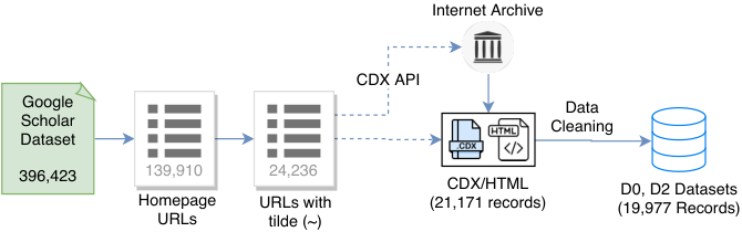
Step 1: From the Google Scholar profile records, we discovered 139,910 profiles that provided homepage URLs. These URLs referenced either individual author homepages, or organizational websites. Since our study focused on modeling the dynamics of the websites of individual authors, we removed organizational websites. This was nontrivial using a simple rule-based filter as there were personal homepages that look similar to organizational homepages. Therefore, we restricted our scope to homepage URLs hosted within a user directory of an institution, i.e., URLs with a tilde () in them (e.g., foo.edu/~bar/). In this manner, we obtained 24,236 homepage URLs.
Step 2: Next, we performed a wildcard query on the IA Wayback CDX Server API [29] to obtain TimeMaps for each author website under their homepage URL. Out of 24,236 websites, we obtained TimeMaps for 21,171 author websites ( archival rate). The remaining websites were either not archived, or the CDX Server API returned an error code during access. The resulting TimeMaps provided information such as the crawl timestamps and URI-Ms of archived copies of each webpage. From these webpages, we selected webpages at depth (Depth 0 is the homepage). For instance, for a homepage foo.edu/~bar, a link to foo.edu/~bar/baz is of depth 1 and is selected. However a link to foo.edu/~bar/baz/qux/quux is of depth 3 and is not selected.
Step 3: Next, we generated the D0 dataset and D2 dataset, which we use in our analysis. First, we de-referenced the URI-Ms of each URL selected in Step 2, and saved their HTML for later use. When doing so, we dropped inconsistent records such as records with invalid checksum, invalid date, multiple depth 0 URLs, and duplicate captures from our data. The resulting data, which we refer to as the D2 dataset, contained HTML of 19,977 websites, totaling 581,603 individual webpages. The average number of webpages per website is 227.49. The minimum and maximum number of webpages per website are 1 and 35,056, respectively. We selected a subset of the D2 dataset consisting HTML of only the 19,977 homepages, which we refer to as the D0 dataset.
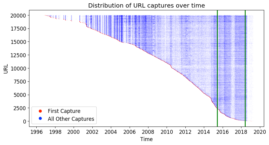
Figure 3 shows the distribution of captures in the D0 dataset, sorted by their earliest capture time. Here, the median crawl interval of of author homepages were between days. The distribution of capture density over time suggests that the capture densities of IA vary irregularly with time. For instance, captures during 2015–2018 show a higher density on average than the captures during 2010–2014. Since high-cadence captures help to obtain a better estimation for the update occurrences, we scoped our analysis to the period between June 1, 2015 and June 1, 2018 (shown by green vertical lines in Figure 3).
II-B Estimating Mean Update Frequency
The exact interpretation of update may differ depending on the purpose of study. We examine a specific type of update – the addition of new links. The intuition here is to identify when authors add new publications into their webpages, as opposed to identifying when that webpage was updated in general. We claim that this interpretation of update is more suited to capture such behavior.
For each webpage in datasets D0 and D2, we processed each capture to extract links from its HTML, where is the set of links in the capture. Next, we calculated , i.e., the number of links in a capture that was never seen before , for each capture in these datasets. Formally,
and is the union of links from captures to . Finally, we calculated the observed-update intervals and observed non-update intervals based on captures that show link additions, i.e., and ones that do not, i.e., (see Figure 1). We estimate in two ways.
II-B1 Estimation Based on Observed Updates
For each webpage, we substituted and values into Eq. (5) or Eq.(4) and solved for using Brent’s method to obtain its estimated mean observed-update frequency (). In this manner, we calculated for author websites at both homepage-level (using D0 dataset) and webpage-level (using D2 dataset).

Figure 4 shows the distribution of at both website-level and homepage-level, obtained using captures from 2015-06-01 to 2018-06-01. Both distributions are approximately log-normal, with a median of days at website-level, and of days at homepage-level. This suggests that most authors add links to their homepage less often than they add links to their website (e.g., publications).
II-B2 Estimation Based on Interpolated Updates
The method described in Section II-B1 calculates the maximum likelihood of observing the updates given by intervals and . Intuitively, an update could have occurred at any time between and , where is the time of an updated capture, and is the time when the capture before it was taken. Here, we use an improved method where we first interpolate when a URL was updated. We define interpolated-update time () as , i.e., the midpoint between and . Next, we obtain the update intervals and from these interpolated updates, and use them to calculate the estimated mean interpolated-update frequency ().
II-C Distribution of Updates


Figure 5 shows the distribution of (red) and the median interpolated-update interval () (blue) of author websites at both homepage-level and website-level. It suggests that the distribution of is consistent with the distribution of median at both homepage-level and website-level.
II-D Poisson Distribution
Next, we observe whether updates to author websites follow a Poisson distribution, at both homepage-level and website-level. Here, we group author websites by their calculated values into bins having a width of 1 day. Within each bin, we calculate the probability (y-axis) of finding an author website having an interpolated-update interval () of days (x-axis).
Figure 6 shows the probability distributions for homepage-level (using D0 dataset) and website-level (using D2 dataset), at days and days, respectively. The majority of data points follow a power-law distribution in the logarithmic scale, indicating that they fit into a Poisson distribution. We also observe that at homepage-level, the data points follow a power-law distribution with a positive index when is (approximately) lower than . We observe sporadic spikes on top of the power law. This indicates that: (1) For a given , consecutive changes within short intervals occur less frequently than predicted by a Poisson distribution, (2) The updates of scholarly webpages are not absolutely random but exhibit a certain level of weak correlation. Investigating the reasons behind these correlations is beyond the scope of this paper, but presumably, they may reflect collaboration or community-level activities. Probability distributions for other values of also exhibit similar patterns (see Figures 15, 16, 17, and 18 in Appendix).
II-E Prediction Model
We formally define our prediction model using two functions, and . The function takes the captures (i.e. crawl snapshots from the IA) of a website as input, and outputs its estimated mean update frequency (See Eq. (5)) and last known update time . The function takes a website’s estimated mean update frequency (), its last known update time (), and a time interval () as input, and outputs the probability () that the website changes after the time interval since its last known update time .
III Evaluation
Here, we study how archived copies of webpages, and the quasi-Poisson distribution of webpage updates can be leveraged to build a focused crawl scheduler for the scholarly web.
Figure 7 illustrates our crawl scheduling model, HACS. For a selected date between 2015-06-01 and 2018-06-01, we first obtain, from the D2 and D0, archived captures of seed URLs within weeks prior to (i.e., in the interval ). Based on these captures, we calculate the estimated mean interpolated-update frequency () of each seed URL. Next, we use the values thus obtained, to calculate the probability () that each seed URL would exhibit a change days from (i.e., by day ). Following this, we sort the seed URLs in the decreasing order of , and apply a threshold parameter () to select a subset of seed URLs to be crawled on that date.
III-A Simulated Crawl Scheduling Task
Here, we set week, and advance across different points in time from 2015-06-01 to 2018-06-01, to simulate a crawl scheduling task. At each , we use standard IR metrics to evaluate whether the selected subset of seed URLs were the ones that actually changed within the interval . We also experiment with different values of (i.e., history size), to determine which yields an optimal result.
The following metrics are used for evaluating our model in comparison with several baseline models. First, we look at precision, recall, and to measure how accurately the scheduler selects URLs for a simulated crawl job (see Evaluation 1). Then, we use @K to evaluate how accurate the scheduler ranks URLs in the order they change (see Evaluation 2).
III-B Evaluation 1
Because most implementations of scholarly web crawlers are not published, we compare with two baseline models, (1) random URLs (Random), and (2) Brute Force (select all URLs). We introduce a threshold parameter to select webpages with a probability of change for crawling. Formally, we define the scheduling function as,
Here, is the set of all seed URLs, and is the set of captures of a seed URL . The parameters , , and are the history size, reference point, and threshold, respectively. The functions and are as defined in Section II-E. For each , the following actions are performed: In the HACS model, we use to select URLs for crawling. In the Random model, we randomly pick URLs from , i.e., all URLs having captures within the time window of . In the Brute Force model, we mimic the behavior of a hypothetical crawler by picking all URLs from . The results from each model were compared to the URLs that actually changed within the interval .
Following this, we counted the number of true positives (TP), true negatives (TN), false positives (FP), and false negatives (FN) at each . Next, we got rid of the reference point by macro/micro-averaging over , and calculated Precision , Recall , and F1 for each and , respectively. At each , we then calculated the threshold which maximizes for both homepage-level and website-level. Table I shows the results from this evaluation.
| Homepage-level | |||||||||
|---|---|---|---|---|---|---|---|---|---|
| Micro Average | Macro Average | ||||||||
| HACS | Random | Brute | HACS | Random | Brute | ||||
| 1 | 0.8 | 0.759 | 0.028 | 0.014 | 0.9 | 0.919 | 0.034 | 0.026 | |
| 2 | 0.7 | 0.367 | 0.020 | 0.021 | 0.8 | 0.647 | 0.018 | 0.026 | |
| 3 | 0.7 | 0.267 | 0.031 | 0.026 | 0.7 | 0.305 | 0.025 | 0.029 | |
| 4 | 0.6 | 0.175 | 0.046 | 0.037 | 0.7 | 0.243 | 0.038 | 0.039 | |
| 5 | 0.6 | 0.178 | 0.053 | 0.044 | 0.7 | 0.220 | 0.047 | 0.046 | |
| 6 | 0.6 | 0.155 | 0.047 | 0.044 | 0.7 | 0.186 | 0.045 | 0.045 | |
| 7 | 0.6 | 0.134 | 0.047 | 0.043 | 0.6 | 0.136 | 0.044 | 0.045 | |
| 8 | 0.6 | 0.124 | 0.046 | 0.043 | 0.6 | 0.125 | 0.044 | 0.045 | |
| 9 | 0.7 | 0.134 | 0.050 | 0.045 | 0.7 | 0.139 | 0.048 | 0.047 | |
| 10 | 0.7 | 0.127 | 0.047 | 0.045 | 0.7 | 0.132 | 0.046 | 0.047 | |
| 11 | 0.7 | 0.121 | 0.047 | 0.045 | 0.7 | 0.125 | 0.046 | 0.047 | |
| 12 | 0.7 | 0.114 | 0.050 | 0.045 | 0.7 | 0.118 | 0.050 | 0.046 | |
| 1 | 0.8 | 0.500 | 0.019 | 1.000 | 0.9 | 0.556 | 0.026 | 1.000 | |
| 2 | 0.7 | 0.332 | 0.018 | 1.000 | 0.8 | 0.321 | 0.007 | 1.000 | |
| 3 | 0.7 | 0.291 | 0.033 | 1.000 | 0.7 | 0.346 | 0.025 | 1.000 | |
| 4 | 0.6 | 0.426 | 0.111 | 1.000 | 0.7 | 0.299 | 0.043 | 1.000 | |
| 5 | 0.6 | 0.445 | 0.133 | 1.000 | 0.7 | 0.322 | 0.070 | 1.000 | |
| 6 | 0.6 | 0.445 | 0.136 | 1.000 | 0.7 | 0.325 | 0.083 | 1.000 | |
| 7 | 0.6 | 0.448 | 0.156 | 1.000 | 0.6 | 0.459 | 0.147 | 1.000 | |
| 8 | 0.6 | 0.454 | 0.168 | 1.000 | 0.6 | 0.466 | 0.164 | 1.000 | |
| 9 | 0.7 | 0.335 | 0.125 | 1.000 | 0.7 | 0.342 | 0.122 | 1.000 | |
| 10 | 0.7 | 0.342 | 0.125 | 1.000 | 0.7 | 0.351 | 0.124 | 1.000 | |
| 11 | 0.7 | 0.348 | 0.134 | 1.000 | 0.7 | 0.356 | 0.134 | 1.000 | |
| 12 | 0.7 | 0.349 | 0.153 | 1.000 | 0.7 | 0.358 | 0.152 | 1.000 | |
| 1 | 1 | 0.8 | 0.603 | 0.022 | 0.028 | 0.9 | 0.750 | 0.678 | 0.044 |
| 2 | 0.7 | 0.349 | 0.019 | 0.041 | 0.8 | 0.420 | 0.221 | 0.048 | |
| 3 | 0.7 | 0.279 | 0.032 | 0.051 | 0.7 | 0.306 | 0.087 | 0.055 | |
| 4 | 0.6 | 0.248 | 0.065 | 0.071 | 0.7 | 0.255 | 0.070 | 0.074 | |
| 5 | 0.6 | 0.254 | 0.076 | 0.084 | 0.7 | 0.253 | 0.071 | 0.087 | |
| 6 | 0.6 | 0.230 | 0.070 | 0.084 | 0.7 | 0.228 | 0.067 | 0.086 | |
| 7 | 0.6 | 0.206 | 0.072 | 0.083 | 0.6 | 0.205 | 0.073 | 0.086 | |
| 8 | 0.6 | 0.194 | 0.072 | 0.082 | 0.6 | 0.194 | 0.071 | 0.086 | |
| 9 | 0.7 | 0.191 | 0.071 | 0.086 | 0.7 | 0.192 | 0.072 | 0.090 | |
| 10 | 0.7 | 0.186 | 0.068 | 0.086 | 0.7 | 0.187 | 0.069 | 0.089 | |
| 11 | 0.7 | 0.180 | 0.069 | 0.086 | 0.7 | 0.181 | 0.067 | 0.089 | |
| 12 | 0.7 | 0.172 | 0.075 | 0.085 | 0.7 | 0.173 | 0.074 | 0.088 | |
| Website-level | |||||||||
|---|---|---|---|---|---|---|---|---|---|
| Micro Average | Macro Average | ||||||||
| HACS | Random | Brute | HACS | Random | Brute | ||||
| 1 | 0.5 | 0.195 | 0.103 | 0.099 | 0.5 | 0.191 | 0.096 | 0.098 | |
| 2 | 0.5 | 0.185 | 0.104 | 0.099 | 0.5 | 0.181 | 0.099 | 0.099 | |
| 3 | 0.5 | 0.164 | 0.099 | 0.096 | 0.5 | 0.162 | 0.095 | 0.096 | |
| 4 | 0.5 | 0.158 | 0.097 | 0.096 | 0.5 | 0.157 | 0.094 | 0.096 | |
| 5 | 0.5 | 0.150 | 0.098 | 0.096 | 0.5 | 0.150 | 0.097 | 0.096 | |
| 6 | 0.5 | 0.139 | 0.094 | 0.092 | 0.5 | 0.139 | 0.093 | 0.093 | |
| 7 | 0.5 | 0.130 | 0.091 | 0.089 | 0.5 | 0.131 | 0.091 | 0.090 | |
| 8 | 0.5 | 0.123 | 0.089 | 0.087 | 0.5 | 0.124 | 0.089 | 0.088 | |
| 9 | 0.5 | 0.118 | 0.087 | 0.085 | 0.5 | 0.120 | 0.088 | 0.087 | |
| 10 | 0.5 | 0.113 | 0.084 | 0.084 | 0.5 | 0.115 | 0.085 | 0.085 | |
| 11 | 0.5 | 0.108 | 0.083 | 0.082 | 0.5 | 0.110 | 0.084 | 0.084 | |
| 12 | 0.5 | 0.104 | 0.081 | 0.080 | 0.5 | 0.106 | 0.082 | 0.082 | |
| 1 | 0.5 | 0.435 | 0.230 | 1.000 | 0.5 | 0.444 | 0.228 | 1.000 | |
| 2 | 0.5 | 0.447 | 0.253 | 1.000 | 0.5 | 0.457 | 0.257 | 1.000 | |
| 3 | 0.5 | 0.460 | 0.277 | 1.000 | 0.5 | 0.471 | 0.280 | 1.000 | |
| 4 | 0.5 | 0.475 | 0.292 | 1.000 | 0.5 | 0.486 | 0.297 | 1.000 | |
| 5 | 0.5 | 0.482 | 0.315 | 1.000 | 0.5 | 0.493 | 0.320 | 1.000 | |
| 6 | 0.5 | 0.488 | 0.329 | 1.000 | 0.5 | 0.498 | 0.334 | 1.000 | |
| 7 | 0.5 | 0.492 | 0.345 | 1.000 | 0.5 | 0.502 | 0.349 | 1.000 | |
| 8 | 0.5 | 0.494 | 0.356 | 1.000 | 0.5 | 0.504 | 0.361 | 1.000 | |
| 9 | 0.5 | 0.497 | 0.367 | 1.000 | 0.5 | 0.507 | 0.373 | 1.000 | |
| 10 | 0.5 | 0.501 | 0.374 | 1.000 | 0.5 | 0.510 | 0.378 | 1.000 | |
| 11 | 0.5 | 0.505 | 0.385 | 1.000 | 0.5 | 0.512 | 0.389 | 1.000 | |
| 12 | 0.5 | 0.507 | 0.393 | 1.000 | 0.5 | 0.514 | 0.397 | 1.000 | |
| 1 | 1 | 0.5 | 0.269 | 0.142 | 0.180 | 0.5 | 0.262 | 0.132 | 0.177 |
| 2 | 0.5 | 0.261 | 0.148 | 0.181 | 0.5 | 0.256 | 0.141 | 0.179 | |
| 3 | 0.5 | 0.242 | 0.145 | 0.175 | 0.5 | 0.238 | 0.140 | 0.174 | |
| 4 | 0.5 | 0.237 | 0.146 | 0.175 | 0.5 | 0.234 | 0.141 | 0.175 | |
| 5 | 0.5 | 0.229 | 0.150 | 0.175 | 0.5 | 0.227 | 0.146 | 0.175 | |
| 6 | 0.5 | 0.216 | 0.146 | 0.168 | 0.5 | 0.215 | 0.143 | 0.169 | |
| 7 | 0.5 | 0.206 | 0.144 | 0.163 | 0.5 | 0.206 | 0.143 | 0.164 | |
| 8 | 0.5 | 0.197 | 0.142 | 0.159 | 0.5 | 0.197 | 0.141 | 0.161 | |
| 9 | 0.5 | 0.191 | 0.141 | 0.157 | 0.5 | 0.192 | 0.140 | 0.159 | |
| 10 | 0.5 | 0.184 | 0.137 | 0.154 | 0.5 | 0.186 | 0.137 | 0.156 | |
| 11 | 0.5 | 0.178 | 0.136 | 0.151 | 0.5 | 0.180 | 0.136 | 0.154 | |
| 12 | 0.5 | 0.173 | 0.134 | 0.149 | 0.5 | 0.175 | 0.134 | 0.151 | |
We also show how , and changes with for both homepage-level and website-level updates. Figures 8,9, and 10 illustrate these results at and (also, results at given in Figures 12, 13, and 14 in Appendix).
III-C Evaluation 2
Here, the HACS model was compared against two baseline models: Last-Obs and Random. In the HACS model, URLs that have a higher probability of change on the crawl date are ranked higher. In the Last-Obs model, URL ranks are determined by the date they were last accessed. Here, URLs that have not been updated the longest (i.e. larger ) are ranked higher. In the Random model, URLs are ranked randomly. By comparing the URL rankings from each model to the expected URL ranking (where URLs that were updated closer to were ranked higher), we calculate a weighted @ over all . Here, the weights were obtained via a logarithmic decay function to increase the contribution from lower values. This weighted @ provides a quantitative measure of whether URLs that were actually updated first were ranked higher. Next, we get rid of the reference point by calculating the mean weighted @ over all , at each history size . In this manner, we obtain the mean weighted @ of each model when different history sizes () are used. Figure 11 shows the results from this evaluation.
IV Results
The results in Table I indicate that the and values of HACS model are higher than the Random and Brute Force models for all values of (history size in weeks). This lead is higher when is lower. However, this difference becomes less significant as increases. The Brute Force method had a consistent of , since it crawls all URLs at all times. However, this model is impractical due to resource constraints. The HACS model produced a higher than the Random model at all . Also, for homepage-level and for website-level indicates the optimal ranges for .
From Figure 8, as increases, the score of HACS model increases until , and then drops as increases further. At , the HACS model yields the highest micro-average score at both the homepage-level and the website-level. This trend is more prominent at the homepage-level than the website-level. In terms of macro-average , the Random model closely follows the HACS model at homepage-level when . However, the HACS model yields better scores in all other cases. The Brute Force model gives constant scores at both homepage-level and website-level, as it selects all seed URLs regardless of .
When comparing precision , Figure 9 shows that both micro-average and macro-average ’s of HACS model increases as increases. This is expected as the URL selection becomes stricter as increases, which, in turn, generates less false positives. Similar to , the lead in of the HACS model is more noticeable at homepage-level than website-level. Nevertheless, the HACS model yields higher than other models in all cases. The Brute Force model has a constant , as it selects all URLs regardless of . However, of Brute Force model is lower than HACS model at both homepage-level and website-level. Interestingly, the of both Brute Force and Random models remain close to each other. At (i.e. when no threshold is applied), all models give the same results, as they select all seed URLs.
When comparing results of , Figure 10 shows that both micro-average and macro-average decreases as increases. This is expected as the URL selection becomes stricter as increases, which, in turn, generates less false negatives. The Brute Force model has a constant of , as it selects all URLs regardless of . At (i.e. when no threshold is applied), all models give as they select all seed URLs. At , both HACS and Random models give , as they select no URLs here. For values other than these, the HACS model consistently yields better than Random model at both homepage-level and website-level. However, this lead is less significant at website-level than at homepage-level, and diminishes as increases.
When comparing the average P@K results, Figure 11 shows that the HACS model yields a better average P@K than the Last-Obs and Random models at both homepage-level and website-level, for all values of . However, the HACS model yields a higher average P@K for lower values of than for higher values of . As increases, the average P@K of all models become approximately constant. At homepage-level, the Last-Obs model yields a better average P@K than the Random model for lower values of . At website-level, however, it yields a worse average P@K than the Random model for higher values of .
V Discussion
From Table I, the , , and values obtained from the HACS model are greater than the baseline models at both the homepage-level and the website-level, when the optimal threshold is selected. Figure 8 shows that regardless of the selected, the HACS model performs better than the baseline models. Also, the of the HACS model increases as increases. This indicates that the HACS model predicted a higher probability () for the URLs that got updated first during . This is also confirmed by the higher mean weighted @ values obtained by the HACS model (see Figure 11). Since decreases with increasing while increases with increasing , it is imperative that an optimal value should be selected. Results in Table I show that selecting (which maximizes ) provides a good compromise between precision and recall, yet perform better than the baseline models.
The and of the Brute Force model is constant irrespective of . Though this model yields the highest (which is ), it consumes a significant amount of resources to crawl everything. This approach does not scale well to a large number of seed URLs. It also yields a lower and than the HACS model across all , at both homepage-level and website-level. These results suggest that the HACS model, which yields a much higher and at a marginal reduction in , is more suited for a resource-constrained environment.
Recall that the archival of webpages is both irregular and sparse (See Figure 3). In our sample, authors updated their homepages every days on average, and their websites every days on average. Note that here, an update to a webpage means adding a new link into it. Authors may update their homepages or websites by updating content or adding external links. Content updates can be studied in a similar way by comparing the checksum of webpages. Since CDX files only contain mementos of webpages within the same domain, taking external links into consideration may require other data sources. The better performance of the HACS model in estimating the mean update frequency for homepages may be attributed to the fact that homepages undergo fewer changes than websites.
From Table I, the best micro-average measure obtained at homepage-level and website-level were and , respectively. Similarly, the best macro-average measures obtained at homepage-level and website-level were and , respectively. In both cases, these measures originated from the HACS model when and .
Figure 8 demonstrates the efficiency of our model. As the threshold increases, the number of false positives is reduced, thereby increasing the precision. Here, we note that even a small increase in precision matters, because for a large number of seed URLs, even the slightest increase in precision attributes to a large decrease in false positives. If crawling is performed on a regular basis, the HACS model could be utilized to pick seed URLs that have most likely been updated. This, based on the above results, would improve collection freshness while using resources and bandwidth more effectively.
VI Conclusion
We studied the problem of improving the efficiency of a focused crawl scheduler for the scholarly web. By analyzing the crawl history of seed URLs obtained from the IA, we fit their change information into a Poisson model and estimated the probability that a webpage would update (addition of new links) by the next crawl. Finally, our scheduler automatically generates a list of seed URLs most likely to have changed since the last crawl. Our analysis found that the estimated mean update frequency (or equivalently, update interval) follow a log-normal distribution. For the 19,977 authors we studied from Google Scholar, new links were added on an average interval of 141.5 days for a homepage, and 75 days for a website. We also observed that the median crawl interval of of author homepages was between 20–127 days. Our evaluation results show that our scheduler achieved better results than the baseline models when is optimized. To encourage reproducible research, our research dataset consisting of HTML, CDX files, and evaluation results have been made publicly available11 1 https://github.com/oduwsdl/scholarly-change-rate.
In the future, we will investigate different types of updates, such as the addition of a scholarly publication in PDF format. Additionally, author websites could be crawled regularly to ensure that updates are not missed, and its effect on the estimation of mean update frequency could be evaluated. We will also generalize this work into more domains by exploring non-scholarly URLs.
VII Acknowledgement
This work was supported in part by the National Science Foundation and the Dominion Graduate Scholarship from the College of Science at the Old Dominion University.
References
- [1] S. Chakrabarti, B. Dom, P. Raghavan, S. Rajagopalan, D. Gibson, and J. Kleinberg, “Automatic resource compilation by analyzing hyperlink structure and associated text,” Computer networks and ISDN systems, vol. 30, no. 1-7, pp. 65–74, 1998.
- [2] S. Chakrabarti, M. Van den Berg, and B. Dom, “Focused crawling: a new approach to topic-specific web resource discovery,” Computer networks, vol. 31, no. 11, pp. 1623–1640, 1999.
- [3] C. Olston and M. Najork, “Web crawling.” Foundations and Trends in Information Retrieval, vol. 4, no. 3, pp. 175–246, 2010.
- [4] B. Tofel, “Wayback’for accessing web archives,” in Proceedings of the 7th International Web Archiving Workshop. IWAW’07, 2007, pp. 27–37.
- [5] D. Gomes, J. a. Miranda, and M. Costa, “A survey on web archiving initiatives,” in Proceedings of Theory and Practice of Digital Libraries (TPDL), 2011, pp. 408–420.
- [6] M. Farrell, E. McCain, M. Praetzellis, G. Thomas, and P. Walker, “Web archiving in the United States: a 2017 survey,” https://osf.io/ht6ay/, 2018.
- [7] H. Van de Sompel, M. L. Nelson, R. Sanderson, L. L. Balakireva, S. Ainsworth, and H. Shankar, “Memento: Time Travel for the Web,” arXiv, Tech. Rep. arXiv:0911.1112, 2009.
- [8] W. Koehler, “Web page change and persistence — a four-year longitudinal study,” Journal of the American Society for Information Science and Technology, vol. 53, no. 2, pp. 162–171, 2002.
- [9] J. Cho and H. Garcia-Molina, “Estimating frequency of change,” ACM Transactions on Internet Technology, vol. 3, no. 3, pp. 256–290, Aug. 2003.
- [10] K. Radinsky and P. Bennett, “Predicting content change on the web,” in WSDM ’13: Proceedings of the Sixth ACM International Conference on Web Search and Data Mining, 2013.
- [11] E. G. Coffman Jr., Z. Liu, and R. R. Weber, “Optimal robot scheduling for web search engines,” Journal of Scheduling, vol. 1, no. 1, pp. 15–29, 1998.
- [12] C. Castillo, M. Marin, A. Rodriguez, and R. Baeza-Yates, “Scheduling algorithms for web crawling,” in WebMedia and LA-Web, 2004. Proceedings. Ribeirao Preto, Brazil: IEEE, Oct. 2004, pp. 10–17.
- [13] P. De Bra, G.-J. Houben, Y. Kornatzky, and R. Post, “Information retrieval in distributed hypertexts,” in Intelligent Multimedia Information Retrieval Systems and Management-Volume 1. Centre de Hautes Etudes Internationales d’inform atique Docum entaire, 1994, pp. 481–491.
- [14] M. Hersovici, M. Jacovi, Y. S. Maarek, D. Pelleg, M. Shtalhaim, and S. Ur, “The shark-search algorithm. an application: tailored web site mapping,” Computer Networks and ISDN Systems, vol. 30, no. 1-7, pp. 317–326, 1998.
- [15] F. Shipman and C. D. D. Monteiro, “Crawling and classification strategies for generating a multi-language corpus of sign language video,” in 19th ACM/IEEE Joint Conference on Digital Libraries, JCDL 2019, 2019, pp. 97–106.
- [16] G. Gossen, E. Demidova, and T. Risse, “icrawl: Improving the freshness of web collections by integrating social web and focused web crawling,” in Proceedings of the 15th ACM/IEEE-CE Joint Conference on Digital Libraries, 2015, pp. 75–84.
- [17] C. Olston and S. Pandey, “Recrawl scheduling based on information longevity,” in Proceedings of the 17th International Conference on World Wide Web, WWW 2008. ACM, 2008.
- [18] J. Cho, H. Garcia-Molina, and L. Page, “Efficient crawling through url ordering,” Computer Networks and ISDN Systems, vol. 30, no. 1-7, pp. 161–172, 1998.
- [19] M. H. Alam, J. Ha, and S. Lee, “Novel approaches to crawling important pages early,” Knowledge and Information Systems, vol. 33, no. 3, pp. 707–734, 2012.
- [20] J. Wu, P. Teregowda, J. P. F. Ramírez, P. Mitra, S. Zheng, and C. L. Giles, “The evolution of a crawling strategy for an academic document search engine: Whitelists and blacklists,” in Proceedings of the 4th Annual ACM Web Science Conference, ser. WebSci ’12, 2012, pp. 340–343.
- [21] S. Zheng, P. Dmitriev, and C. L. Giles, “Graph-based seed selection for web-scale crawlers,” in Proceedings of the 18th ACM Conference on Information and Knowledge Management, CIKM 2009. New York, NY, USA: ACM, 2009, pp. 1967–1970.
- [22] D. S. Hochbaum and A. Pathria, “Analysis of the greedy approach in problems of maximum k-coverage,” Naval Research Logistics (NRL), vol. 45, no. 6, pp. 615–627, 1998.
- [23] M. Thelwall and D. Wilkinson, “Graph structure in three national academic webs: Power laws with anomalies,” Journal of the American Society for Information Science and Technology, vol. 54, no. 8, pp. 706–712, 2003.
- [24] C. L. Giles, K. D. Bollacker, and S. Lawrence, “CiteSeer: An automatic citation indexing system,” in Proceedings of the 3rd ACM International Conference on Digital Libraries, June 23-26, 1998, Pittsburgh, PA, USA, 1998, pp. 89–98.
- [25] J. Wu, K. Kim, and C. L. Giles, “CiteSeerX: 20 years of service to scholarly big data,” in Proceedings of the Conference on Artificial Intelligence for Data Discovery and Reuse, ser. AIDR ’19. New York, NY, USA: Association for Computing Machinery, 2019.
- [26] J. Cho and H. Garcia-Molina, “The evolution of the web and implications for an incremental crawler,” in VLDB 2000, Proceedings of 26th International Conference on Very Large Data Bases, 2000, pp. 200–209.
- [27] ——, “Synchronizing a database to improve freshness,” in Proceedings of the 2000 ACM SIGMOD International Conference on Management of Data, May 16-18, 2000, Dallas, Texas, USA., 2000, pp. 117–128.
- [28] R. P. Brent, “An algorithm with guaranteed convergence for finding a zero of a function,” The Computer Journal, vol. 14, no. 4, pp. 422–425, 1971.
- [29] Internet Archive, “Wayback CDX Server API,” https://github.com/internetarchive/wayback/tree/master/wayback-cdx-server, 2019.
Appendix A Appendix: Supplementary Figures
This section documents additional results obtained from the evaluation of HACS model against our baselines, and the verification of the stochastic nature of scholarly webpage updates for more interval sizes.
Figure 12 illustrates the vs Threshold () of each model, when a history size of 3 weeks is used. Here too, the HACS model produced a higher than other baseline models. This lead is more visible at the homepage-level than the website-level. However, compared to a history size of 1 week and 2 weeks, this lead is less prominent at both homepage-level and webpage-level. As increases, the of the HACS model increases up to , and then drops as further increases. This drop is more visible at the website-level than the homepage-level. The macro-average of Random model follows the HACS model with a similar trend at the Homepage-level, History = 1 week.
Figure 13 illustrates the Precision () vs Threshold () of each model, when a history size of three weeks is used. Here too, the HACS model produced a higher P than the baselines for all values of at homepage level, and for at website level. This lead is more visible at homepage-level than website-level. However, compared to a history size of 1 week and 2 weeks, this lead is less prominent at both homepage-level and webpage-level. Both Random and Brute Force models have a low , regardless of .
Figure 14 illustrates the Recall () vs Threshold () of each model, when a history size of three weeks is used. Here too, the HACS model produced a higher than other baseline models for all values of , at both homepage level and website level. This lead is more visible at homepage-level than website-level. However, compared to a history size of 1 week and 2 weeks, this lead is less prominent at both homepage-level and webpage-level. The Brute Force model has a consistent of , as it selects all seed URLs regardless. The Random model has a low , regardless of .
Figures 15, 16, 17, and 18 illustrates the probability of finding author websites with an interpolated update interval of days for additional values of , ranging from 7 days to 70 days, at both homepage-level (see Figure 15) and webpage-level (see Figure 16). The results suggest that as increases, the probability distribution gets closer to the expected poisson distribution in both cases.