PAC-Learning for Strategic Classification

Ravi Sundaram Affiliation: Khoury College of Computer Science, Northeastern University, Boston, MA 02115 Anil Vullikanti Affiliation: Department of Computer Science, University of Virginia, Charlottesville, VA 22904 Affiliation: Biocomplexity Institute and Initiative, University of Virginia, Charlottesville, VA 22904 Haifeng Xu Affiliation: Department of Computer Science, University of Virginia, Charlottesville, VA 22904 Correspondence to: hx4ad@virginia.edu Fan Yao Affiliation: Department of Computer Science, University of Virginia, Charlottesville, VA 22904 Correspondence to: fy4bc@virginia.edu

Abstract

The study of strategic or adversarial manipulation of testing data to fool a classifier has attracted much recent attention. Most previous works have focused on two extreme situations where any testing data point either is completely adversarial or always equally prefers the positive label. In this paper, we generalize both of these through a unified framework for strategic classification, and introduce the notion of strategic VC-dimension (SVC) to capture the PAC-learnability in our general strategic setup. SVC provably generalizes the recent concept of adversarial VC-dimension (AVC) introduced by Cullina et al. 2018. We instantiate our framework for the fundamental strategic linear classification problem. We fully characterize: (1) the statistical learnability of linear classifiers by pinning down its SVC; (2) its computational tractability by pinning down the complexity of the empirical risk minimization problem. Interestingly, the SVC of linear classifiers is always upper bounded by its standard VC-dimension. This characterization also strictly generalizes the AVC bound for linear classifiers in (Cullina et al. 2018).

Keywords:

Machine Learning, ICML

^†^†affiliationnotice: Equal contribution

1 Introduction

In today’s increasingly connected world, it is rare that an algorithm will act alone. When a machine learning algorithm is used to make predictions or decisions about others who have their own preferences over the learning outcomes, it is well known (e.g., Goodhart’s law) that gaming behaviors may arise—these have been observed in a variety of domains such as finance (Tearsheet), online retailing (Hannak et al. 2014), education (Hardt et al. 2016) as well as during the ongoing COVID-19 pandemic (Bryan & Crossroads; Williams & Haire). In the early months of the pandemic, simple decision rules were designed for COVID-19 testing (COVID) by the CDC. However, people had different preferences for getting tested. Those with work-from-home jobs and leave benefits preferred to get tested in order to know their true health status whereas some of the people with lower income, and without leave benefits preferred not to get tested (with fears of losing their income) (Williams & Haire). Policy makers sometimes prefer to make classification rules confidential (Citron & Pasquale 2014) to mitigate such gaming. However, this is not fool-proof in general since the methods may be reverse engineered in some cases, and transparency of ML methods is sometimes mandated by law, e.g., (Goodman & Flaxman 2016). Such concerns have led to a lot of interest in designing learning algorithms that are robust to strategic gaming behaviors of the data sources (Perote & Perote-Peña 2004; Dekel et al. 2010; Hardt et al. 2016; Chen et al. 2018; Dong et al. 2018; Cullina et al. 2018; Awasthi et al. 2019); the present work subscribes to this literature.

This paper focuses on the ubiquitous binary classification problem, and we look to design classification algorithms that are robust to gaming behaviors during the test phase. We study a strict generalization of the canonical classification setup that naturally incorporates data points’ preferences over classification outcomes (which leads to strategic behaviors as we will describe later). In particular, each data point is denoted as a tuple $(\bm{x},y,r)$ where $\bm{x}\in\mathcal{X}$ and $y\in\{-1,+1\}$ are the feature and label, respectively (as in classic classification problems), and additionally, $r\in\mathbb{R}$ is a real number that describes how much this data point prefers label $+1$ over $-1$ . Importantly, we allow $r$ to be negative, meaning that the data point may prefer label $-1$ . For instance, in the decision rules for COVID-19 testing, individuals who prefer to get tested have $r>0$ , while those who prefer not to be tested have $r<0$ . The magnitude $|r|$ captures how strong their preferences are. For example, in the school choice matching market, students have heterogeneous preferences over universities (Pathak 2017; Roth 2008) and may manipulate their application materials during the admission process. Let set $R\subseteq\mathbb{R}$ denote the set of all possible values that the preference value $r$ may take. Obviously, the trivial singleton set $R=\{0\}$ corresponds to the classic classification setup without any preferences. Another special case of $R=\{1\}$ corresponds to the situation where all data points prefer label $+1$ equally. This is the strategic classification settings studied in several previous works (Hardt et al. 2016; Hu et al. 2019b; Miller et al. 2019). A third special case is $R=\{-1,1\}$ . This corresponds to classification under evasion attacks (Biggio et al. 2013; Goodfellow et al. 2015; Li & Vorobeychik 2014; Cullina et al. 2018; Awasthi et al. 2019), where any test data point $(\bm{x},y)$ prefers the opposite of its true label $y$ , i.e., the “adversarial” assumption.

Our model considers any general preference set $R$ . As we will show, this much richer set of preferences may sometimes make learning more difficult, both statistically and computationally, but not always. Like (Hardt et al. 2016; Dong et al. 2018; Goodfellow et al. 2015; Cullina et al. 2018), our model assumes that manipulation is only possible to the data features and happens only during the test phase. Specifically, the true feature of the test data may be altered by the strategic data point. The cost of masking a true feature $\bm{x}$ to appear as a different feature $\bm{z}$ is captured by a cost function $c(\bm{z};\bm{x})$ . Therefore, the test data point’s decision needs to balance the cost of altering feature and the reward of inducing its preferred label captured by $r$ . As is standard in game-theoretic analysis, the test data point is assumed a rational decision maker and will choose to alter to the feature $\bm{z}$ that maximizes its quasi-linear utility $[r\cdot\mathbb{I}(h(\bm{z})=1)-c(\bm{z};\bm{x})]$ . This naturally gives rise to a Stackelberg game (Von Stackelberg 2010). We aim to learn, from i.i.d. drawn (unaltered) training data, the optimal classifier $h^{*}$ that minimizes the 0-1 classification loss, assuming any randomly drawn test data point (from the same distribution as testing data) will respond to $h^{*}$ strategically. Notably, the data point’s strategic behaviors will not change its true label. Such behavior is referred to as strategic gaming, which crucially differs from strategic improvement studied recently (Kleinberg & Raghavan 2019; Miller et al. 2019).

1.1 Overview of Our Results

The Strategic VC-Dimension. We introduce the novel notion of strategic VC-dimension SVC( $\mathcal{H},R,c$ ) which captures the learnability of any hypothesis class $\mathcal{H}$ when test data points’ strategic behaviors are induced by cost function $c$ and preference values from any set $R\subseteq\mathbb{R}$ .

$\bullet$ We prove that any strategic classification problem is agnostic PAC learnable by the empirical risk minimization paradigm with $O\big(\epsilon^{-2}[d+\log(\frac{1}{\delta}))]\big)$ samples, where $d=$ SVC( $\mathcal{H},R,c$ ). Conceptually, this result illustrates that SVC correctly characterizes the learnability of the hypothesis class $\mathcal{H}$ in our strategic setup.

$\bullet$ Our SVC notion generalizes the adversarial VC-dimension (AVC) introduced in (Cullina et al. 2018) for adversarial learning with evasion attacks. Formally, we prove that AVC equals precisely SVC( $\mathcal{H},R,c$ ) for $R=\{-1,1\}$ when data points are allowed to move within region $\{\bm{z};c(\bm{z};\bm{x})\leq 1\}$ in the corresponding adversarial learning setup. However, for general preference set $R$ , SVC can be arbitrarily larger than both AVC and the standard VC dimension. Thus, complex strategic behaviors may indeed make the learning statistically more difficult. Interestingly, to our knowledge, this is the first time that adversarial learning and strategic learning are unified under the same PAC-learning framework.

$\bullet$ We prove SVC( $\mathcal{H},R,c$ ) $\leq 2$ for any $\mathcal{H}$ and $R$ when $c$ is any separable cost function (introduced by (Hardt et al. 2016)). Invoking our sample complexity results above, this also recovers a main learnability result of (Hardt et al. 2016) and, moreover, generalizes their result to arbitrary agent preferences.

Strategic Linear Classification. As a case study, we instantiate our strategic classification framework in perhaps one of the most fundamental classification problems, linear classification. Here, features are in $\mathbb{R}^{d}$ linear space. We assume the cost function $c(\bm{z};\bm{x})$ for any $\bm{x}$ is induced by arbitrary seminorms of the difference $\bm{z}-\bm{x}$ . We distinguish between two crucial situations: (1) instance-invariant cost function which means the cost of altering the feature $\bm{x}$ to $\bm{x}+\Delta$ is the same for any $\bm{x}$ ; (2) instance-wise cost function which allows the cost from $\bm{x}$ to $\bm{x}+\Delta$ to be different for different $\bm{x}$ . Our results show that the more general instance-wise costs impose significantly more difficulties in terms of both statistical learnability and computational tractability.

$\bullet$ Statistical Learnability. We prove that the SVC of linear classifiers is $\infty$ for instance-wise cost functions even when features are in $\mathbb{R}^{2}$ ; in contrast, the SVC is at most $d+1$ for any instance-independent cost functions and any $R$ when features are in $\mathbb{R}^{d}$ . This later result also strictly generalizes the AVC bound for linear classifiers proved in (Cullina et al. 2018), and illustrates an interesting conceptual message: though SVC can be significantly larger than AVC in general, extending from $R=\{-1,1\}$ (the adversarial setting) to an arbitrary strategic preference set $R$ does not affect the statistical learnability of strategic linear classification.

$\bullet$ Computational Tractability. We show that the empirical risk minimization problem for linear classifier can be solved in polynomial time only when the strategic classification problem exhibits certain adversarial nature. Specifically, an instance is said to have adversarial preferences if all negative test points prefer label $+1$ (but possibly to different extents) and all positive test points prefer label $-1$ . A strictly more relaxed situation has essentially adversarial references — i.e., any negative test point prefers label $+1$ more than any positive test point. We show that for instance-invariant cost functions, any essentially adversarial instance can be solved in polynomial time whereas for instance-wise cost functions, only adversarial instances can be solved in polynomial time. These positive results are essentially the best one can hope for. Indeed, we prove that the following situations, which goes slightly beyond the tractable cases above, are both NP-hard: (1) instance-invariant cost functions but general preferences; (2) instance-wise cost functions but essentially adversarial preferences.

1.2 Related Work and Comparison

Most relevant to ours is perhaps the strategic classification model studied by (Hardt et al. 2016) and (Zhang & Conitzer 2021), where Hardt et al. 2016 formally formulated the strategic classification problem as a repeated Stackelberg game and Zhang & Conitzer 2021 studied the PAC-learning problem and tightly characterized the sample complexity via ”incentive-aware ERM”. However, their model and results all assume homogeneous agent preferences, i.e., all agents equally prefer label $+1$ . Our model strictly generalizes the model of (Hardt et al. 2016; Zhang & Conitzer 2021) by allowing agents’ heterogeneous preferences over classification outcomes. Besides the modeling differences, the research questions we study are also quite different from, and not comparable to, (Hardt et al. 2016). Their positive results are derived under the assumption of separable cost functions or its variants. While our characterization of SVC equaling at most $2$ under separable cost functions implies a PAC-learnability result of (Hardt et al. 2016), this characterization serves more as our case study and our main contribution here is the study of the novel concept of SVC, which does not appear in previous works. Moreover, we study the efficient learnability of linear classifiers with cost functions induced by semi-norms. This broad and natural class of cost functions is not separable, and thus the results of Hardt et al. 2016 does not apply to this case.

Our model also generalizes the setup of adversarial classification with evasion attacks, which has been studied in numerous applications, particularly deep learning models (Biggio et al. 2013; Biggio et al. 2012; Li & Vorobeychik 2014; Carlini & Wagner 2017; Goodfellow et al. 2015; Jagielski et al. 2018; Moosavi-Dezfooli et al. 2017; Mozaffari-Kermani et al. 2015; Rubinstein et al. 2009); however, most of these works do not yield theoretical guarantees. Our work extends and strictly generalizes the recent work of (Cullina et al. 2018) through our more general concept of SVC and results on computational efficiency. In a different work, (Awasthi et al. 2019) studied computationally efficient learning of linear classifiers in adversarial classification with $l_{\infty}$ -norm-induced $\delta$ -ball for allowable adversarial moves. Our computational tractability results generalize their results to $\delta$ -ball induced by arbitrary semi-norms.¹¹ 1 (Awasthi et al. 2019) also studied computational tractability of learning other classes of classifiers, e.g., degree-2 polynomial threshold classifiers, which we do not consider.

Strategic classification has been studied in other different settings or domains or for different purposes, including spam filtering (Brückner & Scheffer 2011), classification under incentive-compatibility constraints (Zhang & Conitzer 2021), online learning (Dong et al. 2018; Chen et al. 2020), and understanding the social implications (Akyol et al. 2016; Milli et al. 2019; Hu et al. 2019b). A relevant but quite different line of recent works study strategic improvements (Kleinberg & Raghavan 2019; Miller et al. 2019; Ustun et al. 2019; Bechavod et al. 2020; Shavit et al. 2020). Finally, going beyond classification, strategic behaviors in machine learning has received significant recent attentions, including in regression problems (Perote & Perote-Peña 2004; Dekel et al. 2010; Chen et al. 2018), distinguishing distributions (Zhang et al. 2019a; Zhang et al. 2019b), and learning for pricing (Amin et al. 2013; Mohri & Munoz 2015; Vanunts & Drutsa 2019). Due to space limit, we refer the curious reader to Appendix A for detailed discussions.

2 Model

Basic Setup. We consider binary classification, where each data point is characterized by a tuple $(\bm{x},y,r)$ . Like classic classification setups, $\bm{x}\in\mathcal{X}$ is the feature vector and $y\in\{+1,-1\}$ is its label. The only difference of our setup from classic classification problems is the additional $r\in R\subseteq\mathbb{R}$ , which is the data point’s (positive or negative) preference/reward of being labeled as $+1$ . The data point’s reward for label $-1$ is, without loss of generality, normalized to be $0$ . A classifier is a mapping $h:\mathcal{X}\to\{+1,-1\}$ . Our model is essentially the same as that of (Hardt et al. 2016; Miller et al. 2019), except that the $r$ in our model can be any real value from set $R$ whereas the aforementioned works assume $r=1$ for all data points. Notably, we also allow $r$ to be negative, which means some data points prefer to be classified as label $-1$ . This generalization is natural and very useful because it allows much richer agent preferences. For instance, it casts the adversarial/robust classification problem as a special case of our model as well (see discussions later). Intuitively, the set $R$ captures the richness of agents’ preferences. As we will prove, how rich it is will affect both the statistical learnability and computational tractability of the learning problem.

Refer to caption — Figure 1: Example illustration of our setup. The line is a linear classifier. Points $\bm{x}_{3},\bm{x}_{4}$ have incentive to cross the boundary whereas $\bm{x}_{1},\bm{x}_{2}$ do not. The dotted cycles contain all manipulated features which have moving cost exactly $1$ and they can be different for different points (i.e., instance-wise costs).

The Strategic Manipulation of Test Data. We consider strategic behaviors during the test phase and assume that the training data is unaltered/uncontaminated. An illustration of the setup can be found in Figure 1. A generic test data point is denoted as $(\bm{x},y,r)$ . The test data point is strategic and may shift its feature to vector $\bm{z}$ with cost $c(\bm{z};\bm{x})$ where $c:\mathcal{X}\times\mathcal{X}\to\mathbb{R}_{\geq 0}$ . In general, function $c$ can be an arbitrary non-negative cost function. In our study of strategic linear classification, we assume the cost functions are induced by seminorms. We will consider the following two types of cost functions, with increasing generality.

1.

Instance-invariant cost functions: A cost function $c$ is instance-invariant if there is a common function $l$ such that $c(\bm{z};\bm{x})=l(\bm{z}-\bm{x})$ for any point $(\bm{x},y,r)$ .
2.

Instance-wise cost functions: A cost function $c$ is instance-wise if for each data point $(\bm{x},y,r)$ , there is a function $l_{\bm{x}}$ such that $c(\bm{z};\bm{x})=l_{\bm{x}}(\bm{z}-\bm{x})$ . Notably, $l_{\bm{x}}$ may be different for different data point $(\bm{x},y,r)$ .

Both cases have been considered in previous works. For instance, the separable cost function studied in (Hardt et al. 2016) is instance-wise, and the cost function induced by a seminorm as assumed by the main theorem of (Cullina et al. 2018) is instance-invariant. We shall prove later that the choice among these two types of cost functions will largely affect the efficient learnability of the problem.

Given a classifier $h$ , the strategic test data point $(\bm{x},y,r)$ may shift its feature vector to $\bm{z}$ and would like to pick the best such $\bm{z}$ by solving the following optimization problem:

		$\displaystyle\text{Data Point Best Response: }$		(1)
		$\displaystyle\Delta_{c}(\bm{x},r;h)=\arg\mathop{max}_{\mathbf{z}\in\mathcal{X}}\big[\mathbb{I}(h(\bm{z})=1)\cdot r-c(\bm{z};\bm{x})\big].$		(1)

where $\mathbb{I}(S)$ is the indicator function and $[\mathbb{I}(h(\bm{z})=1)\cdot r-c(\bm{z};\bm{x})]$ is the quasi-linear utility function of data point $(\bm{x},y,r)$ . We call $\Delta_{c}(\bm{x},r;h)$ the manipulated feature. When there are multiple best responses, we assume the data point may choose any best response and thus will adopt the standard worst-case analysis. Note that the test data’s strategic behaviors do not change its true label. Such strategic gaming behaviors differs from strategic improvements (see (Miller et al. 2019) for more discussions on their differences).

2.1 The Strategic Classification (StraC) Problem

A StraC problem is described by a hypothesis class $\mathcal{H}$ , the set of preferences $R$ and a manipulation cost function $c$ . We thus denote it as StraC $\langle\mathcal{H},R,c\rangle$ . Adopting the standard statistical learning framework, the input to our learning task are $n$ uncontaminated training data points $(\bm{x}_{1},y_{1},r_{1}),\cdots,(\bm{x}_{n},y_{n},r_{n})$ drawn independently and identically (i.i.d.) from distribution $\mathcal{D}$ . Given these training data, we look to learn a classifier $h\in\mathcal{H}$ which minimizes the basic 0-1 loss, defined as follows:

		$\displaystyle\text{Strategic 0-1 Loss of classifier }h:$		(2)
		$\displaystyle L_{c}(h;\mathcal{D})=\mathop{\mathbf{Pr}}_{(\bm{x},y,r)\sim\mathcal{D}}\big[h(\Delta_{c}(\bm{x},r;h))\not=y)\big].$		(2)

Notably, the classifier $h$ in the above loss definition takes the manipulated feature $\Delta_{c}(\bm{x},r;h))$ as input and, nevertheless, looks to correctly predict the true label $y$ . For notational convenience, we sometimes omit $c$ when it is clear from the context and simply write $\Delta(\bm{x},r;h)$ and $L(h;\mathcal{D})$ .

2.2 Notable Special Cases

Our strategic classification model generalizes several models studied in previous literature, which we now sketch.
Non-strategic classification. When $R=\{0\}$ and $c(\bm{z};\bm{x})>0$ for any $\bm{x}\not=\bm{z}$ , our model degenerates to the standard non-strategic setting.
Strategic classification with homogeneous preference. When $R=\{1\}$ , our model degenerates to the strategic classification model studied in prior work (Hardt et al. 2016; Hu et al. 2019b; Milli et al. 2019)—here all data points have the same incentive of being classified as $+1$ .
Adversarial Classification. When $R=\{1,-1\}$ (or $\{\delta,-\delta\}$ , $\delta\neq 0$ ), our model becomes the adversarial classification problem (Cullina et al. 2018; Awasthi et al. 2019), where each data point can adversarially move to induce the opposite of its true label — within the ball of radius $1$ induced by cost function $c$ . Our Proposition 1 provides formal evidence for this connection.
Generalized Adversarial Classification. An interesting generalization of the above adversarial classification setting is that $r<0$ for all data points with true label $+1$ and $r>0$ for all data points with true label $-1$ . This captures the situation where each point has different “power” (decided by $|r|$ ) to play against the classifier. To our knowledge, this generalized setting has not been considered before. Our results yield new efficient statistical learnability and computational tractability for this setting.

3 VC-Dimension for Strategic Classification

In this section, we introduce the notion of strategic VC-dimension (SVC) and show that it properly captures the behaviors of a hypothesis class in the strategic setup introduced above. We then show the connection of SVC with previous studies on both strategic and adversarial learning. Before formally introducing SVC, we first define the shattering coefficients in strategic setups.

Definition 1 (Strategic Shattering Coefficients).

The $n$ ’th shattering coefficient of any strategic classification problem StraC $\langle\mathcal{H},R,c\rangle$ is defined as

	$\displaystyle$	$\displaystyle\sigma_{n}(\mathcal{H},R,c)=\mathop{max}_{\bm{(\bm{x},r)}\in\mathcal{X}^{n}\times R^{n}}$
		$\displaystyle\|\{(h(\Delta_{c}(\bm{x}_{1},r_{1};h)),\cdots,h(\Delta_{c}(\bm{x}_{n},r_{n};h)):h\in\mathcal{H}\}\|,$

where $\Delta_{c}(\bm{x}_{i},r_{i};h)$ defined in Eq. (1) is a best response of data point $(\bm{x}_{i},y_{i},r_{i})$ to classifier $h$ under cost function $c$ .

That is, $\sigma_{n}(\mathcal{H},R,c)$ captures the maximum number of classification behaviors/outcomes (among all choices of data points) that classifiers in $\mathcal{H}$ can possibly induce by using manipulated features as input. Like classic definition of shattering coefficient, the $\sigma_{n}(\mathcal{H},R,c)$ here does not involve the labels of the data points at all. In contrast, in the shattering coefficient definition for adversarial VC-dimension of (Cullina et al. 2018), the “ $\mathop{max}$ ” is allowed to be over data labels as well. This is an important difference from us. Given the definition of the strategic shattering coefficients, the definition of strategic VC-dimension is standard.

Definition 2.

The Strategic VC-dimension (SVC) for strategic classification problem StraC $\langle\mathcal{H},R,c\rangle$ is defined as

\text{SVC}(\mathcal{H},R,c)=\sup\{n\in\mathbb{N}:\sigma_{n}(\mathcal{H},R,c)=2^{n}\}.

(3)

We show that the SVC defined above correctly characterizes the learnability of any strategic classification problem StraC $\langle\mathcal{H},R,c\rangle$ . We consider the standard Empirical risk minimization (ERM) paradigm for strategic classification, but take into account training data’s manipulation behaviors. Specifically, given any cost function $c$ , any $n$ uncontaminated training data points $(\mathbf{x}_{1},y_{1},r_{1}),\cdots,(\mathbf{x}_{n},y_{n},r_{n})$ drawn independently and identically (i.i.d.) from the same distribution $\mathcal{D}$ , the strategic empirical risk minimization (SERM) problem computes a classifier $h\in\mathcal{H}$ that minimizes the empirical strategic 0-1 loss in Eq. (2). Formally, the SERM for StraC $\langle\mathcal{H},R,c\rangle$ is defined as follows:

		$\displaystyle\text{SERM}:\quad\text{argmin}_{h\in\mathcal{H}}\,\,L_{c}(h,\{(\bm{x}_{i},y_{i},r_{i})\}_{i=1}^{n})$		(4)
		$\displaystyle=\sum_{i=1}^{n}\mathbb{I}\big[h(\Delta_{c}(\bm{x}_{i},r_{i};h))\not=y_{i}\big]$		(4)

where $L_{c}(h,\{(\bm{x}_{i},y_{i},r_{i})\}_{i=1}^{n})$ is the empirical loss (compared to the expected loss $L_{c}(h,\mathcal{D})$ defined in Equation (2)). Unlike the standard (non-strategic) ERM problem and similar in spirit to the ”incentive-aware ERM” in (Zhang & Conitzer 2021), classifiers in the SERM problem take each data point’s strategic response $\Delta_{c}\ (\bm{x}_{i},r_{i};h)$ as input, while not the original feature vector $\bm{x}_{i}$ .

Given the definition of strategic VC-dimension and the SERM framework, we state the sample complexity result for PAC-learning in our strategic setup:

Definition 3 (PAC-Learnability).

In a strategic classification problem StraC $\langle\mathcal{H},R,c\rangle$ , the hypothesis class $\mathcal{H}\subseteq(\mathcal{X}\xrightarrow{}\{+1,-1\})$ is Probably Approximately Correctly (PAC) learnable by an algorithm $\mathcal{A}$ if there is a function $m_{\mathcal{H},R,c}:(0,1)^{2}\xrightarrow{}\mathbb{N}$ such that $\forall(\delta,\epsilon)\in(0,1)^{2}$ , for any $n\geq m_{\mathcal{H},R,c}(\delta,\epsilon)$ and any distribution $\mathcal{D}$ for $(\bm{x},y,r)$ , with at least probability $1-\delta$ , we have $L_{c}(h^{*},\mathcal{D})\leq\epsilon$ where $h^{*}$ is the output of the algorithm $\mathcal{A}$ with $n$ i.i.d. samples from $\mathcal{D}$ as input. The problem is agnostic PAC learnable if $L_{c}(h^{*},\mathcal{D})-\inf_{h\in\mathcal{H}}L_{c}(h,\mathcal{D})\leq\epsilon$ .

Theorem 1.

Any strategic classification instance StraC $\langle\mathcal{H},R,c\rangle$ is agnostic PAC learnable with sample complexity $m_{\mathcal{H},R,c}(\delta,\epsilon)\leq C\epsilon^{-2}[d+\log(\frac{1}{\delta})]$ by the SERM in Eq. (4), where $d=SVC(\mathcal{H},R,c)$ is the strategic VC-dimension and $C$ is an absolute constant.

Proof Sketch.

The key idea of the proof is to convert our new strategic learning setup to a standard PAC learning setup, so that the Rademacher complexity argument can be applied. This is done by viewing the preference $r\in R$ as an additional dimension in the augmented feature vector space. Formally, we consider the new binary hypothesis class $\tilde{H}=\{\kappa_{c}(h):h\in H\}$ , where classifier $\kappa_{c}$ satisfies $\kappa_{c}(h):(\bm{x},r)\mapsto h(\Delta_{c}(\bm{x},r;h)),\forall(\bm{x},r)\in\mathcal{X}\times R$ . It turns out that the SVC defined above captures the VC-dimension for this new hypothesis class $\tilde{H}$ . Formally proof can be found in Appendix B.1. ∎

Due to space limit, we defer all formal proofs to the appendix. Proof sketches are provided for some of the results. Next, we illustrate how SVC connects to previous literature, particularly the two most relevant works by Cullina et al. (Cullina et al. 2018) and Hardt et al. (Hardt et al. 2016).

3.1 SVC generalizes Adversarial VC-Dimension (AVC)

We show that SVC generalizes the adversarial VC dimension (AVC) introduced by (Cullina et al. 2018). We give an intuitive description of AVC here, and refer the curious reader to Appendix 1 for its formal definition. At a high level, AVC captures the behaviors of binary classifiers under adversarial manipulations. Such adversarial manipulations are described by a binary nearness relation $\mathcal{B}\subseteq\mathcal{X}\times\mathcal{X}$ and $(\bm{z};\bm{x})\in\mathcal{B}$ if and only if data point with feature $\bm{x}$ can manipulate its feature to $\bm{z}$ . Note that there is no direct notion of agents’ utilities or costs in adversarial classification since each data point simply tries to ruin the classifier by moving within the allowed manipulation region (usually an $\delta$ -ball around the data point). Nevertheless, our next result shows that AVC with binary nearness relation $\mathcal{B}$ always equals to SVC as long as the set of strategic manipulations induced by the data points’ incentives is the same as $\mathcal{B}$ . To formalize our statement, we need the following consistency definition.

Definition 4.

Given any binary relation $\mathcal{B}$ and any cost function $c$ , we say $\mathcal{B},c$ are $r$ -consistent if $\mathcal{B}=\{(\bm{z};\bm{x}):c(\bm{z};\bm{x})\leq r\}$ . In this case, we also say $\mathcal{B}$ [resp. $c$ ] is $r$ -consistent with $c$ [resp. $\mathcal{B}$ ].

By definition any cost function $c$ is $r$ -consistent with the natural binary nearness relation it induces $\mathcal{B}_{c}=\{(\bm{z};\bm{x}):c(\bm{z};\bm{x})\leq r\}$ . Conversely, any binary relation $\mathcal{B}$ is $r$ -consistent (for any $r>0$ ) with a natural cost function that is simply an indicator function of $\mathcal{B}$ defined as follows

c_{\mathcal{B}}(\bm{z};\bm{x})=\begin{cases}\infty,&\text{if }(\bm{z};\bm{x})\in\mathcal{B}\\ 0,&\text{if }(\bm{z};\bm{x})\not\in\mathcal{B}\end{cases}.

(5)

Note that, $\mathcal{B}$ and $c$ may be $r$ -consistent for infinitely many different $r$ , as shown in the above example with $\mathcal{B}$ and $c_{\mathcal{B}}$ .

Proposition 1.

For any hypothesis class $\mathcal{H}$ and any binary nearness relation $\mathcal{B}$ , let AVC $(\mathcal{H},\mathcal{B})$ denote the adversarial VC-dimension defined in (Cullina et al. 2018). Suppose $\mathcal{B}$ and $c$ are $r$ -consistent for some $r>0$ , then we have AVC $(\mathcal{H},\mathcal{B})=$ SVC $(\mathcal{H},\{+r,-r\},c)$ .

As a corollary of Proposition 1, we know that SVC is in general larger than or at least equal to AVC when the strategic behaviors it induces include $\mathcal{B}$ . This is formalized in the following statement.

Corollary 1.1.

Suppose a cost function $c$ is $r$ -consistent with binary nearness relation $\mathcal{B}$ and $\pm r\in R$ , then we have

SVC(\mathcal{H},R,c)\geq AVC(\mathcal{H},\mathcal{B}).

Corollary 1.1 illustrates that for any cost function $c$ , the SVC with a rich preference set $R$ is generally no less than the corresponding AVC under the natural binary nearness relation that $c$ induces. One might wonder how large their gap can be. Our next result shows that for a general $R$ the gap between SVC and AVC can be arbitrarily large even in natural setups. The intrinsic reason is that a general preference set $R$ will lead to different extents of preferences (i.e., some data points strongly prefers label $1$ whereas some slightly prefers it). Such variety of preferences gives rise to more strategic classification outcomes and renders the SVC larger than AVC, and sometimes significantly larger, as shown in the following proposition.

Proposition 2.

For any integer $n>0$ , there exists a hypothesis class $\mathcal{H}$ with point classifiers, an instance-invariant cost function $c(\bm{z};\bm{x})=l(\bm{z}-\bm{x})$ for some metric $c$ and preference set $R$ such that $SVC(\mathcal{H},R,c)=n$ but $VC(\mathcal{H})=AVC(\mathcal{H},\mathcal{B}_{c}(r))=1$ for any $r\in R$ where $\mathcal{B}_{c}(r)=\{(\bm{x},\bm{z}):c(\bm{z};\bm{x})\leq r\}$ is the natural nearness relation induced by $c$ and $r>0$ .

3.2 SVC under Separable Cost Functions

Not only restricting the set $R$ of preference values can reduce the SVC. This subsection shows that restricting to special classes of cost functions can also lead to a small SVC. One special class of cost functions studied in many previous works is the separable cost functions (Hardt et al. 2016; Milli et al. 2019; Hu et al. 2019a). Formally, a cost function $c(\bm{z};\bm{x})$ is separable if there exists function $c_{1},c_{2}:\mathcal{X}\to\mathbb{R}$ such that $c(\bm{z};\bm{x})=\mathop{max}\big\{c_{2}(\bm{z})-c_{1}(\bm{x}),0\big\}$ .

The following Proposition 3 shows that when the cost function is separable, SVC is at most 2 for any hypothesis class $\mathcal{H}$ and any class of preference set $R$ .²² 2 The model of (Hardt et al. 2016) corresponds to the case $R=\{1\}$ in our model. For that restricted situation, the proof of Proposition 3 can be simplified to prove SVC = 1 when $R=\{1\}$ . It turns out that arbitrary preference set $R$ only increases the SVC by at most $1$ . Therefore, separable cost function essentially reduces any classification problem to a problem in lower dimension. Together with Theorem 1, Proposition 3 also recovers the PAC-learnability result of (Hardt et al. 2016) in their strategic-robust learning model (specifically, Theorem 1.8 of (Hardt et al. 2016)) and, moreover, generalizes their learnability from homogeneous agent preferences to the case with arbitrary agent preference values.

Proposition 3.

For any hypothesis class $\mathcal{H}$ , any preference set $R$ satisfying $0\not\in R$ , and any separable cost function $c(\bm{z};\bm{x})$ , we have SVC $(\mathcal{H},R,c)\leq 2$ .

The assumption $0\not\in R$ means each agent must strictly prefer either label $+1$ or $-1$ . This assumption is necessary since if $0\in R$ , SVC will be at least the classic VC dimension of $\mathcal{H}$ and thus Proposition 3 cannot hold. We remark that the above SVC upper bound $2$ holds for any hypothesis class $\mathcal{H}$ . This bound $2$ is tight for some classes of hypothesis, e.g., linear classifiers.

4 Strategic Linear Classification

This section instantiates our previous general framework in one of the most fundamental special cases, i.e., linear classification. We will study both the statistical and computational efficiency in strategic linear classification. Naturally, we will restrict $\mathcal{X}\subseteq\mathbb{R}^{d}$ in this section. Moreover, the cost functions are always assumed to be induced by semi-norms.³³ 3 A function $l:\mathcal{X}\to\mathbb{R}_{\geq 0}$ is a seminorm if it satisfies: (1) triangle inequality: $l(\bm{x}+\bm{z})\leq l(\bm{x})+l(\bm{z})$ for any $\bm{x},\bm{z}\in\mathcal{X}$ ; and (2) homogeneity: $l(\lambda\bm{x})=|\lambda|l(\bm{x})$ for any $\bm{x}\in\mathcal{X},\lambda\in\mathbb{R}$ . A linear classifier is defined by a hyperplane $\bm{w}\cdot\bm{x}+b=0$ ; feature vector $\bm{x}$ is classified as $+1$ if and only if $\bm{w}\cdot\bm{x}+b\geq 0$ . With slight abuse of notation, we sometimes also call $(\bm{w},b)$ a hyperplane or a linear classifier. Let $\mathcal{H}_{d}$ denote the hypothesis set of all $d$ -dimensional linear classifiers. For linear classifier $(\bm{w},b)$ , the data point’s best response can be more explicit expressed as:

\Delta_{c}(x,r;\bm{w},b)=\arg\mathop{max}_{\bm{z}}\big[\mathbb{I}(\bm{w}\cdot\bm{z}+b\geq 0)\cdot r-c(\bm{z};\bm{x})\big].

4.1 Strategic VC-Dimension of Linear Classifiers

We first study the statistical learnability by examining the strategic VC-dimension (SVC). Our first result is a negative one, showing that SVC can be unbounded in general even for linear classifiers with features in $\mathbb{R}^{2}$ (i.e., $\mathcal{X}\subset\mathbb{R}^{2}$ ) and with simple preference set $R=\{+1,-1\}$ .

Theorem 2.

Consider strategic linear classification StraC $\langle\mathcal{H}_{d},R,c\rangle$ . There is an instance-wise cost function $c(\bm{z};\bm{x})=l_{\bm{x}}(\bm{z}-\bm{x})$ where each $l_{\bm{x}}$ is a norm, such that $SVC(\mathcal{H}_{d},R,c)=\infty$ even when $\mathcal{X}\subset\mathbb{R}^{2}$ and $R=\{1\}$ .

Proof Sketch.

We consider a set of data points $\{\bm{x}_{i}\}_{i=1}^{n}$ in $\mathbb{R}^{2}$ whose features are close but with cost functions induced by different norms. The cost functions are designed such that each point $\bm{x}_{i}$ is allowed to strategically alter its feature within a carefully designed polygon $G_{i}$ centered at the origin. Specifically, for any label pattern $\mathcal{L}\in\{+1,-1\}^{n}$ , it has a corresponding node $s_{\mathcal{L}}$ on a unit cycle. The polygon $G_{i}$ for $\bm{x}_{i}$ is the convex hull of all $s_{\mathcal{L}}$ s whose label pattern $\mathcal{L}$ classifies $i$ as $+1$ .

Figure 2 illustrates a high-level idea of our construction. Under such cost functions, we prove that $\mathcal{H}$ can induce all $2^{n}$ possible label patterns. The formal construction and proof can be found in Appendix C. ∎

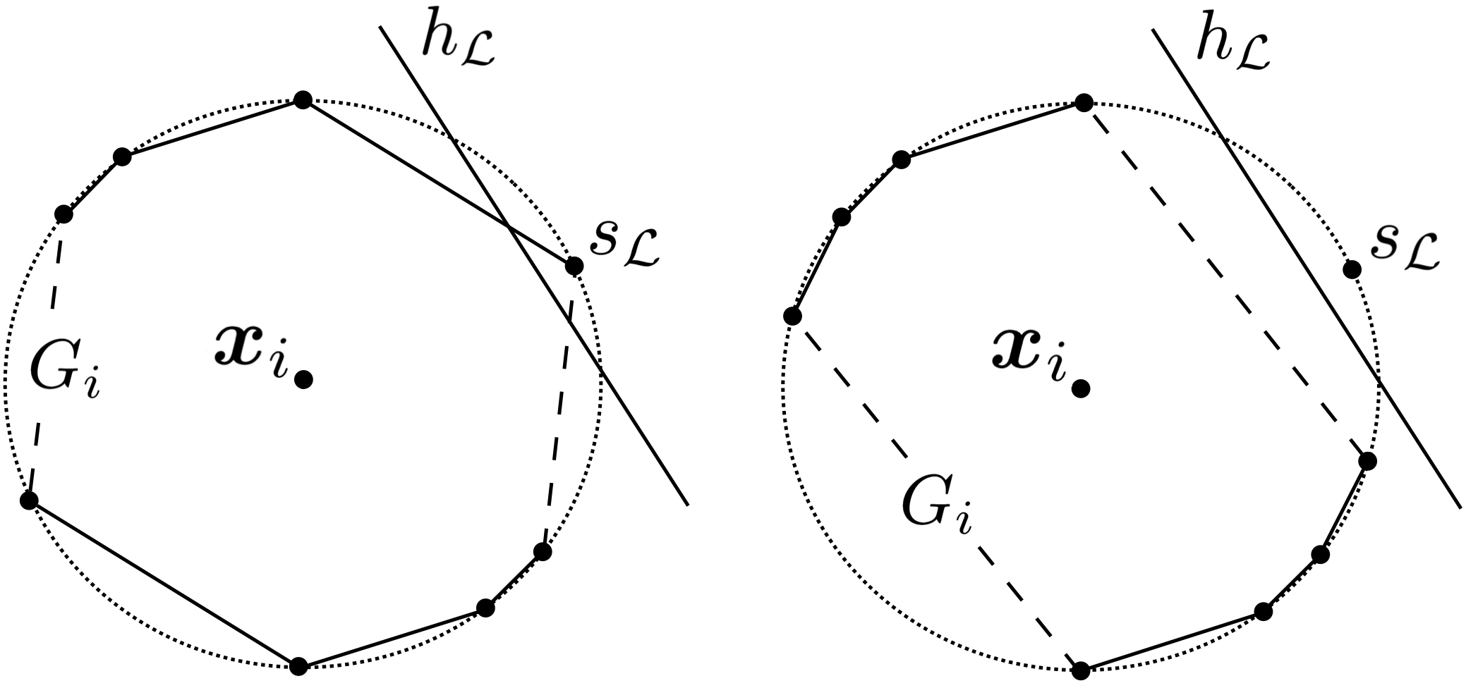
In the study of adversarial VC-dimension (AVC) by (Cullina et al. 2018), the feature manipulation region of each data point is assumed to be instance-invariant. As a corollary, Theorem (2) implies that AVC also becomes $\infty$ for linear classifiers in $\mathbb{R}^{2}$ if each data point’s manipulation region is allowed to be different.

It turns out that the $\infty$ -large SVC above is mainly due to the instance-wise cost functions. Our next result shows that under instance-invariant cost functions, the SVC will behave nicely and, in fact, equal to the AVC for linear classifiers despite the much richer data point manipulation behaviors. This result also strictly generalizes the characterization of AVC by (Cullina et al. 2018) for linear classifiers and shows that linear classifiers will be no harder to learn statistically even allowing richer manipulation preferences of data points.

Theorem 3.

Consider strategic linear classification StraC $\langle\mathcal{H}_{d},R,c\rangle$ . For any instance-invariant cost function $c(\bm{z};\bm{x})=l(\bm{z}-\bm{x})$ where $l$ is a semi-norm, we have SVC $(\mathcal{H}_{d},R,c)=d+1-\dim(V_{l})$ for any bounded $R$ , where $V_{l}$ is the largest linear space contained in the ball $\mathcal{B}=\{\bm{x}:l(\bm{x})\leq 1\}$ .

In particular, if $l$ is a norm (i.e., $l(\bm{x})=0$ iff $\bm{x}=0$ ), then $\dim(V_{l})=0$ and SVC $(\mathcal{H},R,c)=d+1$ .

Proof Sketch.

The key idea of the proof relies on a careful construction of a linear mapping which, given any set of samples $\{(\bm{x}_{i},y_{i},r_{i})\}_{i=1}^{n}$ , maps the class of linear classifiers to the vector space of points’ utilities and moreover, the sign of each data point’s utility will correspond exactly to the label of the data point after its strategic manipulation. Using the structure of this construction, we can identify the relationship between the dimension of the linear mapping and the strategic VC-dimension. By bounding the dimension of the space of signed agent utilities, we are able to derive the SVC though with some involved algebraic argument to exactly pin down the dimension of the linear mapping due to possible degeneracy of $V_{l}$ ball. ∎

4.2 The Complexity of Strategic Linear Classification

In this subsection, we turn our attention to the computational efficiency of learning. The standard ERM problem for linear classification to minimize the 0-1 loss is already known to be NP-hard in the general agnostic learning setting (Feldman et al. 2012). This implies that agnostic PAC learning by SERM is also NP-hard in our strategic setup. Therefore, our computational study will focus on the more interesting PAC-learning case, that is, assuming there exists a strategic linear classifier that perfectly separates all the data points. In the non-strategic case, the ERM problem can be solved easily by a linear feasibility problem.

It turns out that the presence of gaming behaviors does make the resultant SERM problem significantly more challenging. We prove essentially tight computational tractability results in this subsection. Specifically, any strategic linear classification instance can be efficiently PAC-learnable by the SERM when the problem exhibits some “adversarial nature”. However, the SERM problem immediately becomes NP-hard even when we go slightly beyond such adversarial situations. We start by defining what we mean by “adversarial nature” of the problem.

Definition 5 (Essentially Adversarial Instances).

For any strategic classification problem StraC $\langle\mathcal{H},R,c\rangle$ , let

		$\displaystyle\text{ min}^{-}=\mathop{min}\{r:(\bm{x},y,r)\text{ with }y=-1\}\,\,\text{ and }$		(6)
		$\displaystyle\text{max}^{+}=\mathop{max}\{r:(\bm{x},y,r)\text{ with }y=+1\}$		(6)

be the minimum reward among all $-1$ points and the maximum reward among all $+1$ points, respectively. We say the instance is “adversarial” if $\mathop{min}^{-}\geq 0\geq\mathop{max}^{+}$ and is “essentially adversarial” if $\mathop{min}^{-}\geq\mathop{max}^{+}$ .

In other words, an instance is “adversarial” if each data point would like to move to the opposite side of its label though with different magnitudes of preferences, and is “essentially adversarial” if any negative data point has a stronger preference to move to the positive side than any positive data point. Many natural settings are essentially adversarial, e.g., all the four examples in Subsection 2.2.

Our first main result of this subsection (Theorem 4) shows that when the strategic classification problem exhibits the above adversarial nature, linear strategic classification can be efficiently PAC-learnable by SERM. The second main result Theorem 5 shows that the SERM problem becomes NP-hard once we go slightly beyond the adversarial setups identified in Theorem 4. These results show that the computational tractability of strategic classification is primarily governed by the preference set $R$ . Interestingly, this is in contrast to the statistical learnability results in Theorem 2 and 3 where the preference set $R$ did not play much role.

Theorem 4.

Any separable strategic linear classification instance StraC $\langle\mathcal{H}_{d},R,c\rangle$ is efficiently PAC-learnable by the SERM in polynomial time in the following two situations:

1.

The problem is essentially adversarial ( $\mathop{min}^{-}\geq\mathop{max}^{+}$ ) and cost function $c(\bm{z};\bm{x})=l(\bm{z}-\bm{x})$ is instance-invariant and induced by seminorm $l$ .
2.

The problem is adversarial ( $\mathop{min}^{-}\geq 0\geq\mathop{max}^{+}$ ) and the instance-wise cost function $c(\bm{z};\bm{x})=l_{\bm{x}}(\bm{z}-\bm{x})$ is induced by seminorms $l_{\bm{x}}$ .

Proof Sketch.

For situation 1, we can formulate the SERM problem as the following feasibility problem:

\begin{array}[]{lll}\mbox{find}&{\bm{w},b,\epsilon>0}&\\ \mbox{s.t.}&\bm{w}\cdot\bm{x}_{i}+b\geq-r_{i},&\mbox{for }y_{i}=1.\\ &\bm{w}\cdot\bm{x}_{i}+b\leq-(r_{i}+\epsilon),&\mbox{for }y_{i}=-1.\\ &l^{*}(\bm{w})=1&\\ \end{array}

where $l^{*}$ is the dual norm of $l$ .

This unfortunately is not a convex program due to the non-convex constraint $l^{*}(\bm{w})=1$ — indeed we prove later that this program is NP-hard to solve in general. Therefore, instead, we solve a relaxation of the above program, by relaxing constraint $l^{*}(\bm{w})=1$ to $l^{*}(\bm{w})\leq 1$ to obtain a convex program. The crucial step of our proof is to show that this relaxation is tight under the essentially adversarial assumption. This is proved by converting any optimal solution of the relax convex program to a feasible and optimal solution to the original problem. This is the crucial and also difficult step since the solution to the relaxed convex program may not satisfy $l^{*}(\bm{w})=1$ — in fact, it will satisfy $l^{*}(\bm{w})<1$ generally which is why the original program is NP-hard in general. Fortunately, using the essentially adversarial assumption, we are able to employ a carefully crafted construction to generate an optimal solution the the above non-convex program.

For situation 2, we can formulate it as another non-convex program with parameter $\bm{w},\epsilon$ :

\begin{array}[]{lll}\mbox{find}&{\bm{w},b,\epsilon>0}&\\ \mbox{s.t.}&\bm{w}\cdot\bm{x}_{i}+b\geq(-r_{i})\cdot l^{*}_{\bm{x}_{i}}(\bm{w}),&\mbox{for }r_{i}<0.\\ &-(\bm{w}\cdot\bm{x}_{i}+b)\geq(r_{i}+\epsilon)\cdot l^{*}_{\bm{x}_{i}}(\bm{w}),&\mbox{for }r_{i}\geq 0.\\ \end{array}

Fortunately, for any fixed $\epsilon>0$ , the above program is convex in variable $\bm{w}$ . Moreover, if the system is feasible for $\epsilon_{0}>0$ then it is feasible for any $0<\epsilon\leq\epsilon_{0}$ . This allows us to determine the feasibility problem above for any $\epsilon$ via binary search, which overall is in polynomial time. ∎

Our next result shows that the positive claim in Theorem (4) are essentially the best one can hope for. Indeed, the SERM immediately becomes NP-hard if one goes slightly beyond the two tractable situations in Theorem (4). Note that our results did not rule out the possibility of other computationally efficient learning algorithms other than the SERM. We leave this as an intriguing open problem for future works.

Theorem 5.

Suppose the strategic classification problem is linearly separable, then the SERM Problem for linear classifiers is NP-hard in the following two situations:

1.

Preferences are arbitrary and the cost function is instant-invariant and induced by the standard $l_{2}$ norm, i.e., $c(\bm{z};\bm{x})=\|\bm{x}-\bm{z}||_{2}^{2}$ .
2.

The problem is essentially adversarial ( $\mathop{min}^{-}\geq\mathop{max}^{+}$ ) and the cost function is instance-wise and induced by norms.

Remark 1.

Theorem 3, Theorem 4 and Theorem 5 together imply that for strategic linear classification:
(1) the problem is efficiently PAC-learnable (both statistically and computationally) when the cost function is instance-invariant and preferences are essentially adversarial;
(2) SERM can be solved efficiently but SVC is infinitely large when the cost function is instance-wise and preferences are adversarial;
(3) the problem is efficiently PAC learnable in statistical sense, but SERM is NP-hard when the cost function is instance-invariant and preferences are arbitrary.

5 Summary

In this work, we propose and study a general strategic classification setting where data points have different preferences over classification outcomes and different manipulation costs. We establish the PAC-learning framework for this strategic learning setting and characterize both the statistical and computational learnability result for linear classifiers. En route, we generalize the recent characterization of adversarial VC-dimension (Cullina et al. 2018) as well as computational tractability for learning linear classifiers by (Awasthi et al. 2019). Our conclusion reveals two important insights. First, the additional intricacy of having different preferences harms the statistical learnability of general hypothesis classes, but not for linear classifiers. Second, learning strategic linear classifiers can be done efficiently only when the setup exhibits some adversarial nature and becomes NP-hard in general.

Our learnability result for linear classifiers applies to cost functions induced by semi-norms. A future direction is to generalize the theory to cost function induced by asymmetric semi-norms or even any metrics. We also note that the strategic classification model we consider is under the full-information assumption, i.e., the cost function and the strategic preferences are transparent. This is analogous to the evasion attack in the adversarial machine learning literature, where the training data is supposed to be uncontaminated and the manipulation only happens during testing. What if we cannot observe the strategic preferences during training or do not know the adversaries’ cost function? This can be reformulated as online learning through repeated Stackelberg games and has been studied in (Dong et al. 2018), but it does not apply to classifiers with 0-1 loss.

Acknowledgement. We thank anonymous ICML reviewers for helpful suggestions. H. Xu is supported by a GIDI award from the UVA Global Infectious Diseases Institute and a Google Faculty Research Award. A. Vullikanti is supported by NSF grants IIS-1931628, CCF-1918656, NSF IIS-1955797, and NIH grant R01GM109718. R. Sundaram is supported by NSF grants CNS-1718286 and IIS-2039945.

References

Akyol et al. (2016) Akyol, E., Langbort, C., and Basar, T. Price of transparency in strategic machine learning. arXiv, pp. arXiv–1610, 2016.
Amin et al. (2013) Amin, K., Rostamizadeh, A., and Syed, U. Learning prices for repeated auctions with strategic buyers. In Advances in Neural Information Processing Systems, pp. 1169–1177, 2013.
Awasthi et al. (2019) Awasthi, P., Dutta, A., and Vijayaraghavan, A. On robustness to adversarial examples and polynomial optimization. In Advances in Neural Information Processing Systems, pp. 13737–13747, 2019.
Bechavod et al. (2020) Bechavod, Y., Ligett, K., Wu, Z. S., and Ziani, J. Causal feature discovery through strategic modification. arXiv preprint arXiv:2002.07024, 2020.
Biggio et al. (2012) Biggio, B., Nelson, B., and Laskov, P. Poisoning attacks against support vector machines. In Proceedings of the 29th International Coference on International Conference on Machine Learning, ICML’12, pp. 1467–1474, Madison, WI, USA, 2012. Omnipress. ISBN 9781450312851.
Biggio et al. (2013) Biggio, B., Corona, I., Maiorca, D., Nelson, B., Srndic, N., Laskov, P., Giacinto, G., and Roli, F. Evasion attacks against machine learning at test time. In Joint European conference on machine learning and knowledge discovery in databases, pp. 387–402. Springer, 2013.
Brückner & Scheffer (2011) Brückner, M. and Scheffer, T. Stackelberg games for adversarial prediction problems. In Proceedings of the 17th ACM SIGKDD international conference on Knowledge discovery and data mining, pp. 547–555, 2011.
(8) Bryan, M. and Crossroads, K. Coronavirus unemployment benefits are high, putting workers and employers at odds. https://whyy.org/articles/coronavirus-unemployment-benefits-are-high-putting-workers-and-employers-at-odds/.
Carlini & Wagner (2017) Carlini, N. and Wagner, D. Towards evaluating the robustness of neural networks. In 2017 IEEE Symposium on Security and Privacy (SP), pp. 39–57, 2017.
Chen et al. (2018) Chen, Y., Podimata, C., Procaccia, A. D., and Shah, N. Strategyproof linear regression in high dimensions. In Proceedings of the 2018 ACM Conference on Economics and Computation, EC ’18, pp. 9–26, New York, NY, USA, 2018. Association for Computing Machinery. ISBN 9781450358293. doi: 10.1145/3219166.3219175. URL https://doi.org/10.1145/3219166.3219175.
Chen et al. (2020) Chen, Y., Liu, Y., and Podimata, C. Learning strategy-aware linear classifiers. Advances in Neural Information Processing Systems, 33, 2020.
Citron & Pasquale (2014) Citron, D. K. and Pasquale, F. A. The scored society: Due process for automated predictions. 2014.
(13) COVID. Covid-19 testing overview. https://www.cdc.gov/coronavirus/2019-ncov/symptoms-testing/testing.html.
Cullina et al. (2018) Cullina, D., Bhagoji, A. N., and Mittal, P. Pac-learning in the presence of adversaries. In Bengio, S., Wallach, H., Larochelle, H., Grauman, K., Cesa-Bianchi, N., and Garnett, R. (eds.), Advances in Neural Information Processing Systems 31, pp. 230–241. Curran Associates, Inc., 2018.
Dekel et al. (2010) Dekel, O., Fischer, F., and Procaccia, A. D. Incentive compatible regression learning. Journal of Computer and System Sciences, 76(8):759–777, 2010.
Dong et al. (2018) Dong, J., Roth, A., Schutzman, Z., Waggoner, B., and Wu, Z. S. Strategic classification from revealed preferences. In Proceedings of the 2018 ACM Conference on Economics and Computation, EC ’18, pp. 55–70, New York, NY, USA, 2018. Association for Computing Machinery. ISBN 9781450358293. doi: 10.1145/3219166.3219193. URL https://doi.org/10.1145/3219166.3219193.
Feldman et al. (2012) Feldman, V., Guruswami, V., Raghavendra, P., and Wu, Y. Agnostic learning of monomials by halfspaces is hard. SIAM Journal on Computing, 41(6):1558–1590, 2012.
Goodfellow et al. (2015) Goodfellow, I. J., Shlens, J., and Szegedy, C. Explaining and harnessing adversarial examples. In ICLR 2015 : International Conference on Learning Representations 2015, 2015.
Goodman & Flaxman (2016) Goodman, B. and Flaxman, S. EU regulations on algorithmic decision-making and a “right to explanation”, 2016. URL http://arxiv.org/abs/1606.08813. Presented at 2016 ICML Workshop on Human Interpretability in Machine Learning (WHI 2016), New York, NY.
Hannak et al. (2014) Hannak, A., Soeller, G., Lazer, D., Mislove, A., and Wilson, C. Measuring price discrimination and steering on e-commerce web sites. In Proceedings of the 2014 conference on internet measurement conference, pp. 305–318, 2014.
Hardt et al. (2016) Hardt, M., Megiddo, N., Papadimitriou, C., and Wootters, M. Strategic classification. In Proceedings of the 2016 ACM Conference on Innovations in Theoretical Computer Science, ITCS ’16, pp. 111–122, New York, NY, USA, 2016. Association for Computing Machinery. ISBN 9781450340571. doi: 10.1145/2840728.2840730. URL https://doi.org/10.1145/2840728.2840730.
Hu et al. (2019a) Hu, L., Immorlica, N., and Vaughan, J. W. The disparate effects of strategic manipulation. In Proceedings of the Conference on Fairness, Accountability, and Transparency, pp. 259–268, 2019a.
Hu et al. (2019b) Hu, L., Immorlica, N., and Vaughan, J. W. The disparate effects of strategic manipulation. In Proceedings of the Conference on Fairness, Accountability, and Transparency, FAT* ’19, pp. 259–268, New York, NY, USA, 2019b. Association for Computing Machinery. ISBN 9781450361255. doi: 10.1145/3287560.3287597. URL https://doi.org/10.1145/3287560.3287597.
Jagielski et al. (2018) Jagielski, M., Oprea, A., Biggio, B., Liu, C., Nita-Rotaru, C., and Li, B. Manipulating machine learning: Poisoning attacks and countermeasures for regression learning. 2018 IEEE Symposium on Security and Privacy (SP), pp. 19–35, 2018.
Kleinberg & Raghavan (2019) Kleinberg, J. and Raghavan, M. How do classifiers induce agents to invest effort strategically? In Proceedings of the 2019 ACM Conference on Economics and Computation, pp. 825–844, 2019.
Li & Vorobeychik (2014) Li, B. and Vorobeychik, Y. Feature cross-substitution in adversarial classification. In Advances in neural information processing systems, pp. 2087–2095, 2014.
Miller et al. (2019) Miller, J., Milli, S., and Hardt, M. Strategic classification is causal modeling in disguise. arXiv, pp. arXiv–1910, 2019.
Milli et al. (2019) Milli, S., Miller, J., Dragan, A. D., and Hardt, M. The social cost of strategic classification. In Proceedings of the Conference on Fairness, Accountability, and Transparency, FAT* ’19, pp. 230–239, New York, NY, USA, 2019. Association for Computing Machinery. ISBN 9781450361255. doi: 10.1145/3287560.3287576. URL https://doi.org/10.1145/3287560.3287576.
Mohri & Munoz (2015) Mohri, M. and Munoz, A. Revenue optimization against strategic buyers. In Advances in Neural Information Processing Systems, pp. 2530–2538, 2015.
Moosavi-Dezfooli et al. (2017) Moosavi-Dezfooli, S., Fawzi, A., Fawzi, O., and Frossard, P. Universal adversarial perturbations. In 2017 IEEE Conference on Computer Vision and Pattern Recognition (CVPR), pp. 86–94, 2017.
Mozaffari-Kermani et al. (2015) Mozaffari-Kermani, M., Sur-Kolay, S., Raghunathan, A., and Jha, N. K. Systematic poisoning attacks on and defenses for machine learning in healthcare. IEEE Journal of Biomedical and Health Informatics, 19(6):1893–1905, 2015.
Pathak (2017) Pathak, P. A. What really matters in designing school choice mechanisms. Advances in Economics and Econometrics, 1:176–214, 2017.
Perote & Perote-Peña (2004) Perote, J. and Perote-Peña, J. Strategy-proof estimators for simple regression. Math. Soc. Sci., 47:153–176, 2004.
Roth (2008) Roth, A. E. What have we learned from market design? Innovations: Technology, Governance, Globalization, 3(1):119–147, 2008.
Rubinstein et al. (2009) Rubinstein, B. I., Nelson, B., Huang, L., Joseph, A. D., Lau, S.-h., Rao, S., Taft, N., and Tygar, J. D. Stealthy poisoning attacks on pca-based anomaly detectors. SIGMETRICS Perform. Eval. Rev., 37(2):73–74, October 2009. ISSN 0163-5999. doi: 10.1145/1639562.1639592. URL https://doi.org/10.1145/1639562.1639592.
Shalev-Shwartz & Ben-David (2014) Shalev-Shwartz, S. and Ben-David, S. Understanding machine learning: From theory to algorithms. Cambridge university press, 2014.
Shavit et al. (2020) Shavit, Y., Edelman, B., and Axelrod, B. Causal strategic linear regression. In III, H. D. and Singh, A. (eds.), Proceedings of the 37th International Conference on Machine Learning, volume 119 of Proceedings of Machine Learning Research, pp. 8676–8686, 2020.
(38) Tearsheet. Gaming the system: Loan applicants are reverse engineering the online lending algorithms. https://tearsheet.co/data/gaming-the-system-online-loan-applicants-are-reverse-engineering-the-algorithms/.
Ustun et al. (2019) Ustun, B., Spangher, A., and Liu, Y. Actionable recourse in linear classification. In Proceedings of the Conference on Fairness, Accountability, and Transparency, pp. 10–19, 2019.
Vanunts & Drutsa (2019) Vanunts, A. and Drutsa, A. Optimal pricing in repeated posted-price auctions with different patience of the seller and the buyer. In Advances in Neural Information Processing Systems, pp. 939–951, 2019.
Von Stackelberg (2010) Von Stackelberg, H. Market structure and equilibrium. Springer Science & Business Media, 2010.
(42) Williams, J. and Haire, B. Why some people don’t want to take a covid-19 test. https://theconversation.com/why-some-people-dont-want-to-take-a-covid-19-test-141794.
Zhang & Conitzer (2021) Zhang, H. and Conitzer, V. Incentive-aware pac learning. AAAI 2021, 2021.
Zhang et al. (2019a) Zhang, H., Cheng, Y., and Conitzer, V. Distinguishing distributions when samples are strategically transformed. In Advances in Neural Information Processing Systems, pp. 3193–3201, 2019a.
Zhang et al. (2019b) Zhang, H., Cheng, Y., and Conitzer, V. When samples are strategically selected. In International Conference on Machine Learning, pp. 7345–7353, 2019b.

Appendix A Additional discussion on related work

The work of (Hardt et al. 2016) is most relevant to our work—they introduced a Stackelberg game framework to model the interaction between the learner and the test data. Our model can be viewed as a generalization of (Hardt et al. 2016) by allowing heterogeneous preferences over classification outcomes. (Hardt et al. 2016) assume a special class of separably cost functions, and prove that the optimal classifier is always a threshold classifier. Essentially, the assumption of separable cost functions reduces the feature space to a low dimension, which is also why the strategic VC dimension in this case is at most $2$ as we proved. Despite this clean characterization, it appears a strong and somewhat unrealistic requirement. For example, one consequence of separable cost functions is that for any two features $\bm{x},\bm{z}$ , the manipulation cost from either $\bm{x}$ to $\bm{z}$ or from $\bm{z}$ to $\bm{x}$ must be $0$ .⁴⁴ 4 A cost function $c(\bm{z};\bm{x})$ is separable if there exists two functions $c_{1},c_{2}:\mathcal{X}\to\mathbb{R}$ such that $c(\bm{z};\bm{x})=\mathop{max}\{c_{2}(\bm{z})-c_{1}(\bm{x}),0\}$ . Since $c(\bm{x};\bm{x})=0$ , we have $c_{2}(\bm{x})\leq c_{1}(\bm{x})$ for any $\bm{x}$ . Therefore, $c_{2}(\bm{x})+c_{2}(\bm{z})-c_{1}(\bm{x})-c_{1}(\bm{z})\leq 0$ . Consequently, either $c_{2}(\bm{x})-c_{1}(\bm{z})\leq 0$ or $c_{2}(\bm{z})-c_{1}(\bm{x})\leq 0$ , yielding either $c(\bm{z};\bm{x})=0$ or $c(\bm{x};\bm{z})=0$ . This appears unrealistic in reality. For example, a high-school student with true average math grade $80$ and true average literature grade $95$ is likely to incur cost if she/he wants to appear as $95$ for math and $80$ for literature, and vice versa. This is because different students are good at different aspects. Our model imposes less assumptions on the cost functions. For example, in our study of strategic linear classification, the cost functions are induced by arbitrary semi-norms.

(Brückner & Scheffer 2011) is one of the first to consider the Stackelberg game formulation of strategic classification, motivated by spam filtering; however they do not study generalization bounds. (Zhang & Conitzer 2021) provide the sample complexity result for strategic PAC-learning under the homogeneous preference setting and in particular study the case under the incentive-compatibility constraints, i.e., subject to no data points will misreport features. These two works all assume the positive labels are always and equally preferred. There has also been work on understanding the social implications of strategically robust classification (Akyol et al. 2016; Milli et al. 2019; Hu et al. 2019b); these works show that improving the learner’s performance may lead to increased social burden and unfairness. (Dong et al. 2018; Chen et al. 2020) extend strategic linear classification to an online setting where the input features are not known a-priori, but instead are revealed in an online manner. They both focused on the optimization problem of regret minimization. Our setting however is in the more canonical PAC-learning setup and our objective is to design statistically and computationally efficient learning algorithms. All these aforementioned works, including the present work, consider gaming behaviors. A relevant but quite different line of recent works study strategic improvements where the manipulation does really change the inherent quality and labels (Kleinberg & Raghavan 2019; Miller et al. 2019; Ustun et al. 2019; Bechavod et al. 2020; Shavit et al. 2020). The question there is mainly to design incentive mechanisms to encourage agents’ efforts or improvements.

Finally, going beyond classification, strategic behaviors in machine learning has received significant recent attentions, including in regression problems (Perote & Perote-Peña 2004; Dekel et al. 2010; Chen et al. 2018), distinguising distributions (Zhang et al. 2019a; Zhang et al. 2019b), and learning for pricing (Amin et al. 2013; Mohri & Munoz 2015; Vanunts & Drutsa 2019). These are similar in spirit to us, but study a completely different set of problems using different techniques. Their results are not comparable to ours.

Appendix B Omitted Proofs from Section 3

B.1 Proof of Theorem 1

Proof.

Let $\mathcal{Y}=\{+1,-1\}$ . Define another binary hypothesis class $\tilde{H}=\{\kappa_{c}(h):h\in H\}$ , where $\kappa_{c}:(\mathcal{X}\xrightarrow{}\mathcal{Y})\xrightarrow{}(\mathcal{X}\times R\xrightarrow{}\mathcal{Y})$ is a mapping such that $\kappa_{c}(h)(\bm{x},r)=h(\Delta_{c}(\bm{x},r;h)),\forall(\bm{x},r)\in\mathcal{X}\times R$ . Note that the input of classifier $\kappa_{c}(h)$ consists of both the feature vector $\bm{x}$ and the preference $r$ . By the definition of SVC, we have VC $(\tilde{H})=$ SVC $(\mathcal{H},R,c)=d$ .

Given any distribution $\mathcal{D}$ , cost function $c$ , and $h\in\mathcal{H}$ , the strategic 0-1 loss of $h$ is $L_{c}(h,\mathcal{D})=\mathbb{E}_{(\bm{x},y,r)\sim\mathcal{D}}\Big[\mathbb{I}\big[\kappa_{c}(h)(\bm{x},r)\not=y\big]\Big]=L(\kappa_{c}(h),\mathcal{D})$ , where $L(\tilde{h},\mathcal{D})$ is the standard expected risk of the newly defined $\tilde{h}\in\tilde{\mathcal{H}}$ under the distribution $\mathcal{D}$ in the non-strategic setting. Therefore, studying the PAC sample complexity upper bound for $\mathcal{H}$ under the strategic setting $\langle R,c\rangle$ is equivalent to studying the sample complexity for $\tilde{H}$ in the non-strategic setting. The latter problem can be addressed by employing the standard PAC learning analysis. From the Fundamental Theorem of Statistical Learning (Theorem 6.8 in (Shalev-Shwartz & Ben-David 2014)), we know $\tilde{H}$ is agnostic PAC learnable with sample complexity $O(\epsilon^{-2}(\text{VC}(\tilde{H})+\log\frac{1}{\delta}))$ , meaning that there exists a constant $C$ such that for any $(\delta,\epsilon)\in(0,1)^{2}$ and any distribution $\mathcal{D}$ for $(\bm{x},y,r)$ , as long as $n\geq C\cdot\epsilon^{-2}(\text{VC}(\tilde{H})+\log\frac{1}{\delta})$ , with at least probability $1-\delta$ , we have

L(\tilde{h}^{*},\mathcal{D})-\inf_{\tilde{h}\in\tilde{H}}L(\tilde{h},\mathcal{D})\leq\epsilon,

where $\tilde{h}^{*}$ is the solution of ERM with $n$ i.i.d. samples from $\mathcal{D}$ as input. Let $h^{*}$ be the solution of the corresponding SERM conditioned on the same $n$ i.i.d. samples from $\mathcal{D}$ . By the definition of $\tilde{H}$ and $L_{c}$ , we have $L_{c}(h^{*},\mathcal{D})=L(\tilde{h}^{*},\mathcal{D})$ , and $\inf_{h\in\mathcal{H}}L_{c}(h,\mathcal{D})=\inf_{\tilde{h}\in\tilde{H}}L(\tilde{h},\mathcal{D})$ . Therefore, with probability $1-\delta$ , we have

\displaystyle L_{c}(h^{*},\mathcal{D})-\inf_{h\in\mathcal{H}}L_{c}(h,\mathcal{D})\leq\epsilon,

which implies StraC $\langle\mathcal{H},R,c\rangle$ is agnostic PAC learnable with sample complexity $O(\epsilon^{-2}[d+\log(\frac{1}{\delta})])$ by the SERM.

∎

B.2 Proof of Proposition 1

Proof.

The adversarial VC-dimension defined in (Cullina et al. 2018) relies on an auxiliary definition of corrupted classifier $\tilde{h}=\kappa_{R}(h)$ of any classifier $h$ for the standard non-adversarial setting such that $\tilde{h}(\bm{x})=h(\bm{x})$ if all the points in $N(\bm{x})$ have the same label as $\bm{x}$ and otherwise, $\tilde{h}(\bm{x})=\perp$ . Recall that $N(\bm{x})=\{\bm{z}\in\mathcal{X}:(\bm{z};\bm{x})\in\mathcal{B}\}=\{\bm{z}\in\mathcal{X}:c(\bm{z};\bm{x})\leq r\}$ denotes the set of all possible adversarial features $\bm{x}$ can move to. Given this auxiliary definition, the adversarial VC-dimension is defined as AVC $(\mathcal{H},\mathcal{B})=\sup\{n:\sigma_{n}(\mathcal{F},\mathcal{B})=2^{n}\}$ , where

\sigma_{n}(\mathcal{F},\mathcal{B})=\mathop{max}_{(\bm{x},\bm{y})\in\mathcal{X}^{n}\times\{+1,-1\}^{n}}|\{(f(\bm{x}_{1},y_{1};h),\ldots,f(\bm{x}_{n},y_{n};h)):h\in\mathcal{H}\}|

(7)

is the shattering coefficient, and $f(\bm{x}_{i},y_{i})=\mathbb{I}(\tilde{h}(\bm{x}_{i})\neq y_{i})$ is the loss function of the corrupted classifier $\tilde{h}=\kappa_{R}(h)$ .

Since $\mathcal{B}$ and $c$ are $r$ -consistent, we have $\mathcal{B}=\{(\bm{z};\bm{x}):c(\bm{z};\bm{x})\leq r\}$ . Let $R=\{+r,-r\}$ . We now prove the proposition by arguing

\sup\{n\in\mathbb{N}:\sigma_{n}(\mathcal{H},R,c)=2^{n}\}=\sup\{n:\sigma_{n}(\mathcal{F},\mathcal{B})=2^{n}\}.

(8)

1.

If $\sup\{n\in\mathbb{N}:\sigma_{n}(\mathcal{H},R,c)=2^{n}\}=n$ , by Definition 1, there exists $(\bm{x}^{\prime}_{i},r^{\prime}_{i})\in\mathcal{X}\times R,i=1,\cdots,n$ such that $|\{(h(\Delta_{c}(\bm{x}^{\prime}_{1},r^{\prime}_{1};h)),\cdots,h(\Delta_{c}(\bm{x}^{\prime}_{n},r^{\prime}_{n};h)):h\in\mathcal{H}\}|=2^{n}$ . Since Definition 1 does not rely on the true labels of $\bm{x}^{\prime}_{i}$ , we may let the true labels of $\bm{x}^{\prime}_{i}$ be $y^{\prime}_{i}=-r^{\prime}_{i}/r$ for any $i$ . In this case, each $\bm{x}^{\prime}_{i}$ ’s strategic preference is against its true label, which corresponds to the loss function $f$ in Equation (7) for the adversarial setting. Therefore, taking $(\bm{x}_{i},y_{i})=(\bm{x}^{\prime}_{i},y^{\prime}_{i})$ in Equation (7) gives $\sigma_{n}(\mathcal{F},\mathcal{B})=2^{n}$ . This implies $\sup\{n\in\mathbb{N}:\sigma_{n}(\mathcal{H},R,c)=2^{n}\}\leq\sup\{n:\sigma_{n}(\mathcal{F},\mathcal{B})=2^{n}\}$ .
2.

Conversely, if $\sup\{n:\sigma_{n}(\mathcal{F},\mathcal{B})=2^{n}\}=n$ , from Equation (7), there exists $(\bm{x}_{i},y_{i})\in\mathcal{X}\times R,i=1,\cdots,n$ such that $|\{(f(\bm{x}_{1},y_{1}),\ldots,f(\bm{x}_{n},y_{n})):f\in\mathcal{F}\}|=2^{n}.$ Similarly, taking $r_{i}=-ry_{i}\in R$ gives $\sigma_{n}(\mathcal{H},R,c)=2^{n}$ , which implies $\sup\{n\in\mathbb{N}:\sigma_{n}(\mathcal{H},R,c)=2^{n}\}\geq\sup\{n:\sigma_{n}(\mathcal{F},\mathcal{B})=2^{n}\}$ .

Therefore, we have AVC $(\mathcal{H},\mathcal{B})=$ SVC $(\mathcal{H},\{+r,-r\},c)$ for any $r$ -consistent pair $(\mathcal{B},c)$ . ∎

B.3 Proof of Corollary 1.1

Proof.

Since $\{+r,-r\}\subseteq\mathcal{B}$ , we have $\sigma_{n}(\mathcal{H},R,c)\geq\sigma_{n}(\mathcal{H},\{+r,-r\},c)$ by Definition 1. As a result, SVC $(\mathcal{H},R,c)\geq$ SVC $(\mathcal{H},\{+r,-r\},c)$ . Then by applying Proposition 1 we have
SVC $(\mathcal{H},R,c)\geq$ SVC $(\mathcal{H},\{+r,-r\},c)=$ AVC $(\mathcal{H},\mathcal{B})$ . ∎

B.4 Proof of Proposition 2

Given any positive integer $n$ , let $[n]$ denotes $\{1,2,\cdots,n\}$ , and $\mathcal{S}$ be the power set of $[n]$ , i.e., the set that contains all the subsets of $[n]$ . Let $\mathcal{X}=[n]\cup\mathcal{S}$ be the sample space of size $n+2^{n}$ , and the hypothesis class $\mathcal{H}$ is the set of all the point classifiers with points from $\mathcal{S}$ , i.e., $\mathcal{H}=\{h_{s}:s\in\mathcal{S}\}$ , where point classifier $h_{s}$ only classifies the point $s\in\mathcal{S}$ as positive. The cost function $c(z;x)$ is a metric defined as follows. Since metric is symmetric, i.e., $c(z;x)=c(x;z)$ , we will use the notation $c(x,z)$ instead throughout this proof.

c(x,z)=\begin{cases}x,&\text{if}\quad x\in[n],z\in\mathcal{S},x\in z\\ x+1,&\text{if}\quad x\in[n],z\in\mathcal{S},x\notin z\\ c(z,x),&\text{if}\quad x\in\mathcal{S},z\in[n]\\ x+z,&\text{if}\quad x,z\in[n],x\neq z\\ 1,&\text{if}\quad x,z\in\mathcal{S},x\neq z\\ 0,&\text{if}\quad x=z,\end{cases}

(9)

and $R$ is set to be $[-n,-1]\cup[1,n]$ .

First, we verify that $c(\cdot,\cdot)$ is indeed a metric. Given the Definition (9), it is easy to see that $c(x,z)=0$ iff $x=z$ , and $c(x,z)=c(z,x),\forall x,z\in\mathcal{X}$ . It remains to check the triangle inequality, i.e., for any $x,y,z\in\mathcal{X}$ , $c(x,y)+c(y,z)\geq c(x,z)$ . Consider the case when $x,y,z$ are different elements in $\mathcal{X}$ . By enumerating all the possibility that whether each $x,y,z$ is in $[n]$ or $\mathcal{S}$ , it suffices to discuss the following $8(=2^{3})$ cases:

1.

if $x,y,z\in[n]$ , $c(x,y)+c(y,z)=x+y+y+z>x+z=c(x,z)$ .
2.

if $x,y,z\in\mathcal{S}$ , $c(x,y)+c(y,z)=2>1=c(x,z)$ .
3.

if $x,z\in[n],y\in\mathcal{S}$ , then $c(x,y)\geq x,c(y,z)\geq z$ . $\Longrightarrow$ $c(x,y)+c(y,z)\geq x+z=c(x,z)$ .
4.

if $x,y\in[n],z\in\mathcal{S}$ , we need to show that $c(x,y)\geq c(x,z)-c(y,z)$ . Conditioned on the relationship between $x,y$ and set $z$ , the maximum value of $c(x,z)-c(y,z)$ is $x-y+1$ when $y\in z,x\notin z$ . Therefore, $c(x,y)=x+y\geq x-y+1\geq c(x,z)-c(y,z)$ .
5.

if $x,z\in\mathcal{S},y\in[n]$ , then $c(x,y)+c(y,z)\geq y+y>1\geq c(x,z).$
6.

if $x,y\in\mathcal{S},z\in[n]$ , then the maximum value for $c(x,z)-c(y,z)$ is $z+1-z=1$ when $z\notin x,z\in y$ . Therefore, $c(x,y)\geq 1\geq c(x,z)-c(y,z).$
7.

if $x\in\mathcal{S},y,z\in[n]$ , it is equivalent to case 4.
8.

if $y,z\in\mathcal{S},x\in[n]$ , it is equivalent to case 6.

Next, we show VC $(\mathcal{H})=1$ , AVC $(\mathcal{H},\mathcal{B}_{c}(r))=1$ , and SVC $(\mathcal{H},R,c)\geq n$ . Observe that VC $(\mathcal{H})=1$ follows easily since no point classifier $h_{s}\in\mathcal{H}$ can generate the label pattern $(+1,+1)$ for any pair of distinct data points.

Next we prove AVC $(\mathcal{H},\mathcal{B}_{c}(r))=1$ . We first show AVC $(\mathcal{H},\mathcal{B}_{c}(r))\leq 1$ by arguing that under binary nearness relation $\mathcal{B}_{c}(r)=\{(z;x):c(z,x)\leq r\}$ with $r\geq 1$ , any two elements $x_{1},x_{2}$ in $\mathcal{X}$ cannot be shattered by $\mathcal{H}$ .

1.

If at least one of $r_{1},r_{2}$ equals $-r$ , e.g., $r_{1}=-r$ , we show that $x_{1}$ can never be classified as $+1$ by contradiction. Suppose some $h_{s}\in\mathcal{H}$ classifies $(x_{1},-r)$ as $+1$ : if $x_{1}\neq s$ , since $r_{1}=-r<0$ , $x_{1}$ will not manipulate its feature and be classified as $-1$ ; if $x_{1}=s$ , $x_{1}$ can move to any $z\in\mathcal{S}$ with cost $1\leq r$ , and will also be classified as $-1$ . Therefore, $(x_{1},x_{2})$ can not be shattered.
2.
If $r_{1}=r_{2}=r$ , consider the following two cases:
1. (a)
  
  If at least one of $x_{1},x_{2}$ belongs to $\mathcal{S}$ , e.g., $x_{1}\in\mathcal{S}$ , then $x_{1}$ can move to any $s\in\mathcal{S}$ as $c(x_{1},s)=1\leq r$ for any $s\in\mathcal{S}$ . Therefore $x_{1}$ can never be classified as $-1$ by any point classifier in $\mathcal{H}$ .
2. (b)
  
  if $x_{1},x_{2}\in[n]$ , we may w.l.o.g. assume $x_{1}<x_{2}$ , i.e., $x_{1}+1\leq x_{2}$ . Observe that when $r<x_{1}$ , any $h_{s}\in\mathcal{H}$ will classify $x_{1}$ as -1 because $c(x_{1},s)=x_{1}>r,\forall s\in\mathcal{S}$ ; when $r\geq x_{1}+1$ , any $h_{s}\in\mathcal{H}$ will classify $x_{1}$ as +1 because $c(x_{1},s)=x_{1}+1\leq r,\forall s\in\mathcal{S}$ . Therefore, in order to shatter $(x_{1},x_{2})$ , $r$ must lie in the interval $[x_{1},x_{1}+1)\cap[x_{2},x_{2}+1)=\emptyset$ , which draws the contradiction.

To see that AVC $(\mathcal{H},\mathcal{B}_{c}(r))\geq 1$ , for any $x\in[n]$ with $r>0$ , it can be classified as either $+1$ or $-1$ as long as $r\in[x,x+1)$ . We thus have AVC $(\mathcal{H},c)=1$ .

Finally, we prove that SVC $(\mathcal{H},R,c)=n$ . Consider the subset $[n]\subset\mathcal{X}$ of size $n$ , with each element $i$ equipped with a strategic preference $r_{i}=i$ . For any label pattern $\mathcal{L}\in\{+1,-1\}^{n}$ , let $s_{\mathcal{L}}=\{i\in[n]:\mathcal{L}_{i}=+1\}$ be an element in $\mathcal{S}$ . We claim that $h_{s_{\mathcal{L}}}\in\mathcal{H}$ gives exactly the label pattern $\mathcal{L}$ on $[n]$ . To see this, consider any $i\in[n]$ :

1.

If $i\in s_{\mathcal{L}}$ , $i$ will move to $s_{\mathcal{L}}\in\mathcal{S}$ and be classified as $+1$ , as the cost $c(i,s_{\mathcal{L}})=i\leq r_{i}=i$ .
2.

If $i\notin s_{\mathcal{L}}$ , $i$ will not move to $s_{\mathcal{L}}\in\mathcal{S}$ and be classified as $-1$ , as the cost $c(i,s_{\mathcal{L}})=i+1>r_{i}=i$ .

Therefore, any label pattern $\mathcal{L}\in\{+1,-1\}^{n}$ can be achieved by some $h_{s_{\mathcal{L}}}\in\mathcal{H}$ . This implies SVC $(\mathcal{H},R,c)\geq n$ . On the other hand, it’s easy to see $\mathcal{H}$ cannot shatter $n+1$ points, because any subset of size $n+1$ must contain an element $s_{0}$ in $\mathcal{S}$ , and no matter what strategic preference $s_{0}$ has, it will either be classified as $+1$ by all $h_{s}\in\mathcal{H}$ , or be classified as $+1$ by only one classifier in $\mathcal{H}$ , i.e., $h_{s_{0}}$ . Either case renders the shattering for $n+1$ points impossible.

B.5 Proof of Proposition 3

Proof.

Define the adversarial region for an adversary $(\bm{x},r)$ as $N(\bm{x},r)=\{\bm{z}\in\mathcal{X}:c_{2}(\bm{z})\leq c_{1}(\bm{x})+|r|\}\supseteq\{\bm{x}\}$ . Since staying with the same feature has no cost, this implies $c(\bm{x};\bm{x})=0$ or equivalently $c_{2}(\bm{x})\leq c_{1}(\bm{x})$ for any $\bm{x}\in\mathcal{X}$ . Then, the best response function for $(\bm{x},r)$ can be characterized by

1.

if $h(\bm{x})=\text{sgn}(r)$ , then $h(\Delta(\bm{x},r;h))=\text{sgn}(r)$ ;

if $h(\bm{x})=-\text{sgn}(r)$ , then

h(\Delta(\bm{x},r;h))=\begin{cases}-\text{sgn}(r),\quad\forall\bm{z}\in N(\bm{x},r):h(\bm{z})=-\text{sgn}(r)\\ \text{sgn}(r),\quad\exists\bm{z}\in N(\bm{x},r):h(\bm{z})=\text{sgn}(r)\end{cases}

(10)

Suppose there are three points $\{(x_{i},r_{i})\}_{i=1}^{3}$ that can be shattered by $\mathcal{H}$ . Let $b_{i}=c_{1}(\bm{x}_{i})+r_{i}$ and w.l.o.g. let $b_{1}\leq b_{2}\leq b_{3}$ . From $b_{1}\leq b_{2}\leq b_{3}$ , we have $N(\bm{x}_{1},r_{1})\subseteq N(\bm{x}_{2},r_{2})\subseteq N(\bm{x}_{3},r_{3})$ .

By Pigeonhole principle, there must exists two elements in $\{r_{1},r_{2},r_{3}\}$ which have the same sign. Suppose these two elements are $r_{1},r_{2}$ and consider the following two cases:

1.

$r_{1}>0,r_{2}>0$ . From Equation 10, for any $h\in\mathcal{H}$ , $h(\Delta(\bm{x}_{2},r_{2};h))=-1$ means $h(\bm{z})=-1,\forall\bm{z}\in N(\bm{x}_{2},r_{2})$ . Note that $N(\bm{x}_{1},r_{1})\subseteq N(\bm{x}_{2},r_{2})$ , we also have $h(\bm{z})=-1,\forall\bm{z}\in N(\bm{x}_{1},r_{1})$ . As a result, $h(\Delta(\bm{x}_{1},r_{1};h))=-1$ , meaning the sign pattern $\{+,-\}$ cannot be achieved by any $h\in\mathcal{H}$ for $\{(\bm{x}_{1},r_{1}),(\bm{x}_{2},r_{2})\}$ .
2.

$r_{1}<0,r_{2}<0$ . From Equation 10, for any $h\in\mathcal{H}$ , $h(\Delta(\bm{x}_{2},r_{2};h))=1$ means $h(\bm{z})=1,\forall\bm{z}\in N(\bm{x}_{2},r_{2})$ . Similarly, from $N(\bm{x}_{1},r_{1})\subseteq N(\bm{x}_{2},r_{2})$ we conclude $h(\bm{z})=1,\forall\bm{z}\in N(\bm{x}_{1},r_{1})$ and $h(\Delta(\bm{x}_{1},r_{1};h))=1$ , meaning the sign pattern $\{-,+\}$ cannot be achieved by any $h\in\mathcal{H}$ for $\{(\bm{x}_{1},r_{1}),(\bm{x}_{2},r_{2})\}$ .

Therefore, $\{(x_{i},r_{i})\}_{i=1}^{3}$ cannot be shattered by $\mathcal{H}$ , which implies SVC $(\mathcal{H},R,c)\leq 2$ .

∎

Appendix C Proof of Theorem 2

Proof.

Let $\mathcal{X}=\mathbb{R}^{2}$ , and consider the linear hypothesis class on $\mathcal{X}$ : $\mathcal{H}=\{h=\text{sgn}(\bm{w}\cdot\bm{x}+b):(\bm{w},b)\in\mathbb{R}^{3},\bm{x}\in\mathcal{X}\}$ . We show that for any $n\in\mathbb{Z}^{+}$ and $R=\{+1\}$ , there exist $n$ points $\{\bm{x}_{i}\}_{i=1}^{n}\in\mathcal{X}^{n}$ and corresponding cost functions $\{c_{i}\}_{i=1}^{n}$ , such that the $n$ ’th shattering coefficients $\sigma_{n}(\mathcal{H},R,\{c_{i}\}_{i=1}^{n})=2^{n}$ (see Definition 1 for $\sigma_{n}$ ). Note that the cost function is instance-wise. For convenience, here we equivalently think of it as each data point $i$ has a different cost function $c_{i}$ .

Let $\bm{x}_{i}=(0,0),\forall i\in[n]$ be the set of data points. The main challenge of the proof is a very careful construction of the cost function for each data point. To do so, we first pick a set of $2^{n}$ different points $S=\{s_{j}\}_{j=1}^{2^{n}}$ lying on the unit circle, i.e., $S\subset\{(x,y):x^{2}+y^{2}=1\}$ . The number $2^{n}$ is not arbitrarily chosen — indeed, we will map each point $s_{j}$ to one of the $2^{n}$ subsets of $[n]$ in a bijective manner so that each $s_{j}$ corresponds to a unique subset of $[n]$ . What are these $2^{n}$ different points will not matter to our construction neither it matters which point is mapped to which subset so long as it is a bijection. Moreover, let $\bar{S}=\{(-x,-y):(x,y)\in S\}$ be the set that is origin-symmetric to $S$ such that $\bar{S}\cap S=\emptyset$ . $\bar{S}$ is chosen to “symmetrize” our construction to obtain a norm and needs not to have any interpretation. For any $\bm{x}_{i}$ , we now define its cost function $c_{i}$ through the following steps :

1.

Let $S_{i}=\{s\subseteq[n]:i\in s\}\subset S$ contains all the $2^{n-1}$ subsets of $[n]$ that include the element $i$ .
2.

Let $\bar{S}_{i}=\{(-x,-y):(x,y)\in S_{i}\}\subseteq\bar{S}$ be the set that is origin-symmetric to $S_{i}$ .
3.

Let $G_{i}$ be the convex, origin-symmetric polygon with the vertex set being $S_{i}\cup\bar{S}_{i}$ .
4.

The cost function of $\bm{x}_{i}$ is defined as $c_{i}(\bm{z};\bm{x})=\|\bm{x}-\bm{z}\|_{G_{i}}$ , where $\|\cdot\|_{G_{i}}=\inf\{\epsilon\in\mathbb{R}_{\geq 0}:x\in\epsilon G_{i}\}$ is a norm derived from polygon $G_{i}$ (note the origin-symmetry of $S_{i}\cup\bar{S}_{i}$ and thus $G_{i}$ ).

Next we show that for any label pattern $\mathcal{L}\in\{+1,-1\}^{n}$ , there exists some linear classifier $h\in\mathcal{H}_{2}$ such that $(h(\Delta_{c_{1}}(\bm{x}_{1},+1;h),\cdots,h(\Delta_{c_{n}}(\bm{x}_{n},+1;h))=\mathcal{L}$ .

With slight abuse of notation, let $s_{\mathcal{L}}=\{i\in[n]:\mathcal{L}_{i}=+1\}\in S$ be the point in $S$ that corresponds to the set of the indexes of $\mathcal{L}$ with $\mathcal{L}_{i}=1$ . Let $h_{\mathcal{L}}$ be any linear classifier whose decision boundary intersects the unit circle centered at $\bm{x}_{i}$ and strictly separates $s_{\mathcal{L}}$ from all the other elements in $S\cup\bar{S}$ . We will use $h_{\mathcal{L}}$ to denote both the linear classifier and its decision boundary (i.e., a line in $\mathbb{R}^{2}$ ) interchangeably. Due to the convexity of $G_{i}$ , such $h_{\mathcal{L}}$ must exist. We further let $h_{\mathcal{L}}$ give prediction result $+1$ for the half plane that contains $s_{\mathcal{L}}$ and $-1$ for the other half plane. Figure 3 illustrates the geometry of this example.

We now argue that $h_{\mathcal{L}}$ induces the given label pattern $\mathcal{L}$ for instances $\{(\bm{x}_{i},1,c_{i})\}_{i=1}^{n}$ . To see this, we examine $h_{\mathcal{L}}(\Delta_{c_{i}}(\bm{x}_{i},1;h))$ for each $i$ :

1.

If $i\in s_{\mathcal{L}}$ , then $s_{\mathcal{L}}\in S_{i}$ and $\bm{x}_{i}$ can move to $s_{\mathcal{L}}$ with cost $c_{i}(s_{\mathcal{L}};\bm{x}_{i})<1$ . This is because $G_{i}$ is convex and there exist a point $\bm{x}^{\prime}_{i}$ on $h_{\mathcal{L}}$ such that $c_{i}(\bm{x}^{\prime}_{i};\bm{x}_{i})<c_{i}(s_{\mathcal{L}};x_{i})=1=r_{i}$ (e.g., choose $\bm{x}^{\prime}_{i}$ as the intersection point of the segment $[\bm{x}_{i},s_{\mathcal{L}}]$ and $h_{\mathcal{L}}$ ). Therefore, $h_{\mathcal{L}}$ will classify $\bm{x}_{i}$ as positive. This case is shown in the left panel of Figure 3.
2.

If $i\notin s_{\mathcal{L}}$ , then $s_{\mathcal{L}}\notin S_{i}$ and $G_{i}$ does not intersect $h_{\mathcal{L}}$ . In this case, $h_{\mathcal{L}}(\bm{x})=-1$ , and moving across $h_{\mathcal{L}}$ always induces a cost strictly larger than $1$ . Therefore, the best response for $\bm{x}_{i}$ is to stay put and $h_{\mathcal{L}}$ will classify $\bm{x}_{i}$ as negative. This case is shown in the right panel of Figure 3.

Now we have shown that the $n$ ’th shattering coefficients $\sigma_{n}(\mathcal{H},\{+1,-1\},\{c_{i}\}_{i=1}^{n})=2^{n}$ . Since $n$ can take any integer, we conclude the strategic VC-dimension in this case is $+\infty$ .

∎

Appendix D Proof of Theorem 3

The following lemma from advanced linear algebra is widely known and will be useful for our analysis.

Lemma 1.

For any seminorm $l:\mathbb{R}^{d}\xrightarrow{}\mathbb{R}_{\geq 0}$ , and the cost function $c(\bm{z};\bm{x})=l(\bm{z}-\bm{x})$ induced by $l$ , the minimum manipulation cost for $\bm{x}$ to move to the hyperplane $\bm{w}\cdot\bm{x}+b=0$ is given by the following:

\mathop{min}_{\bm{x}^{\prime}}\{c(\bm{x}^{\prime};\bm{x}):\bm{w}\cdot\bm{x}^{\prime}+b=0\}=\frac{|\bm{w}\cdot\bm{x}+b|}{l^{*}(\bm{w})}

where $l^{*}(\bm{w})=\sup_{\bm{z}\in B}\{\bm{w}\cdot\bm{z}\}\in\mathbb{R}_{\geq 0}\cup\{+\infty\}$ , and $\mathcal{B}=\{\bm{z}:l(\bm{z})\leq 1\}$ is the unit ball induced by $l$ .

The proof is divided into the following two parts. The first part is the more involved one.

Proof of SVC $(\mathcal{H}_{d},R,c)\leq d+1-\dim(V_{l})$ :

It suffices to show that for any $n>d+1-\dim(V_{l})$ and $n$ data points $(\bm{x}_{i},r_{i})\in\mathbb{R}^{d}\times R,\forall i=1,\cdots,n$ , there exists a label pattern $\mathcal{L}\in\{+1,-1\}^{n},$ such that for any $h\in\mathcal{H}_{d}$ cannot induce $\mathcal{L}$ , i.e.,

(h(\Delta_{c}(\bm{x}_{1},r_{1};h),\cdots,h(\Delta_{c}(\bm{x}_{n},r_{n};h)))\neq\mathcal{L}.

The first step of our proof derives a succinct characterization about the classification outcome for a set of data points. For any seminorm $l$ , it is known the set $\mathcal{B}=\{x:l(x)\leq 1\}$ is nonempty, closed, convex, and origin-symmetric. Let $l^{*}(\bm{w})=\sup_{\bm{z}\in B}\{\bm{w}\cdot\bm{z}\}$ . We have $l^{*}(\bm{w})>0$ for all $\bm{w}\neq\bm{0}$ since $\bm{0}$ is an interior point of $\mathcal{B}$ . According to Lemma 1, for any $\bm{x}\in\mathbb{R}^{d}$ and any linear classifier $h=(\bm{w},b)\in\mathcal{H}_{d}$ , the minimum manipulation cost for $\bm{x}$ to move to the decision boundary of $h$ is $|\bm{w}\cdot\bm{x}+b|/l^{*}(\bm{w})$ . Note that we may w.l.o.g. restrict to $\bm{w}$ ’s such that $l^{*}(\bm{w})=1$ since the sign function $\text{sgn}(\bm{w}\cdot\bm{x}+b)$ does not change after re-scaling. For any data point $(\bm{x},r)\in\mathcal{X}\times R$ and linear classifier $h\in\mathcal{H}_{d}$ , we define the signed manipulation cost to the classification boundary as

\displaystyle\delta(h,\bm{x})=h(\bm{x})\cdot\frac{|\bm{w}\cdot\bm{x}+b|}{l^{*}(\bm{w})}=\bm{w}\cdot\bm{x}+b,

using the condition $l^{*}(\bm{w})=1$ . We claim that $h(\Delta_{c}(\bm{x},r;h))=2\mathbb{I}(\bm{w}\cdot\bm{x}+b\geq-r)-1$ . This follows a case analysis:

1.

If $r\leq 0$ , then $h(\Delta_{c}(\bm{x},r,h))=1$ if and only if $h(\bm{x})=1$ and $\bm{x}$ cannot move across the decision boundary of $h$ within cost $|r|=-r$ . This implies $h(\Delta_{c}(\bm{x},r;h))=2\mathbb{I}(\bm{w}\cdot\bm{x}+b\geq-r)-1$ .
2.

If $r>0$ , then $h(\Delta_{c}(\bm{x},r,h))=-1$ if and only if $h(\bm{x})=-1$ and $\bm{x}$ cannot move across the decision boundary of $h$ within cost $r$ . In this case, $h(\Delta_{c}(\bm{x},r;h))=-(2\mathbb{I}(-(\bm{w}\cdot\bm{x}+b)>r)-1)=2\mathbb{I}(\bm{w}\cdot\bm{x}+b\geq-r)-1$ . Note that the first inequality holds strictly because we assume $h$ always gives $+1$ for those $\bm{x}$ on the decision boundary.

For a set of samples $(\bm{X},\bm{\bm{r}})$ where $\bm{X}=(\bm{x}_{1},\cdots,\bm{x}_{n}),\bm{\bm{r}}=(r_{1},\cdots,r_{n})$ , define the set of all possible vectors (over the choice of linear classifiers $(\bm{w},b)\in\mathcal{H}_{d}$ ) of signed manipulation costs as

\mathcal{D}(\mathcal{H}_{d},\bm{X})=\{(\bm{w}\cdot\bm{x}_{1}+b,\cdots,\bm{w}\cdot\bm{x}_{n}+b):h\in\mathcal{H}_{d}\},

(11)

there is a $h\in\mathcal{H}_{d}$ that achieves a label pattern $\mathcal{L}$ on $(\bm{X},\bm{r})$ if and only if there exist an element in $D(\mathcal{H}_{d},\bm{\bm{x}})+\bm{\bm{r}}$ with the corresponding sign pattern $\mathcal{L}$ .

Recall that a linear classifier is described by $(\bm{w},b)\in\mathbb{R}^{d+1}$ . The second step of our proof rules out “trivial” linear classifiers under strategic behaviors, and consequently allows us to work with only linear classifiers in a linear space of smaller dimension. Let $\mathcal{B}=\{\bm{x}:l(\bm{x})\leq 1\}$ and $V_{l}$ be the largest linear space contained in $\mathcal{B}$ . We argue that it suffice to consider only linear classifiers $(\bm{w},b)$ with $\bm{w}\perp V_{l}$ . This is because for any $\bm{w}$ that is not orthogonal to the subspace $V_{l}$ , we can find $\bar{\bm{z}}\in V_{l}$ such that $c(\bar{\bm{z}};\bm{x})=0$ and $\bm{w}\cdot\bar{\bm{z}}\to\infty$ since $V_{l}$ is a linear subspace. This means any data point can induce its preferred label $\text{sgn}(r)$ with $0$ cost, by moving to $\bar{\bm{z}}$ if $\text{sgn}(r)=+$ and $-\bar{\bm{z}}$ otherwise. Any such linear classifier will result in the same label pattern, simply specified by $\text{sgn}(r)$ . As a consequence, we only need to focus on linear classifiers $(\bm{w},b)$ with $\bm{w}\perp V_{l}$ . Let $\tilde{H_{d}}=\{(\bm{w},b):\bm{w}\perp V_{l}\}$ denote all such linear classifiers.

Next, we argue that when restricting to the non-trivial class of linear classifiers $\tilde{\mathcal{H}_{d}}$ , the $\mathcal{D}(\tilde{\mathcal{H}_{d}},\bm{X})$ defined in Equation (11) lies in a linear subspace with dimension at most $d+1-\text{dim}(V_{l})$ . Consider the linear mapping $\mathcal{G}_{\bm{X}}:\tilde{\mathcal{H}_{d}}\to\mathbb{R}^{n}$ determined by the data features $\bm{X}$ , defined as

\mathcal{G}_{\bm{X}}(\bm{w},b)=(\bm{w}\cdot\bm{x}_{1}+b,\cdots,\bm{w}\cdot\bm{x}_{n}+b),\quad\forall(\bm{w},b)\in\tilde{\mathcal{H}_{d}}.

Since $\bm{w}\perp V_{l}$ , $\bm{w}$ is from a linear subspace of $d-\text{dim}(V_{l})$ . Linear mapping will not increase the dimension of the image space, therefore $\mathcal{D}(\tilde{\mathcal{H}_{d}},\bm{X})$ lies in a space with dimension at most $d+1-\text{dim}(V_{l})$ .

Finally, we prove that there must exist label patterns that cannot be induced by linear classifiers whenever the number of data points $n>d+1-\dim(V_{l})$ . Let $\text{span}\big(\mathcal{D}(\tilde{\mathcal{H}_{d}},\bm{X})\big)$ denote the smallest linear space that contains $\mathcal{D}(\tilde{\mathcal{H}_{d}},\bm{X})$ . Since $\text{span}\big(\mathcal{D}(\tilde{\mathcal{H}_{d}},\bm{X})\big)$ has dimension at most $d+1-\text{dim}(V_{l})<n$ but $\text{span}\big(\mathcal{D}(\tilde{\mathcal{H}_{d}},\bm{X})\big)\subset\mathbb{R}^{n}$ , there must exist a non-zero vector $\bar{\bm{u}}\in\mathbb{R}^{n}$ such that: (1) $\bar{\bm{u}}\not=\bm{0}$ ; (2) $\bar{\bm{u}}\perp\text{span}\big(\mathcal{D}(\tilde{\mathcal{H}_{d}},\bm{X})\big)$ (i.e., $\bar{\bm{u}}\cdot\bm{v}=0,\forall\bm{v}\in\text{span}\big(\mathcal{D}(\tilde{\mathcal{H}_{d}},\bm{X})\big)$ ); and (3) $\bar{\bm{u}}\cdot\bm{\bm{r}}\leq 0$ (if $\bar{\bm{u}}\cdot\bm{\bm{r}}\geq 0$ , simply takes its negation). Note that this implies $\bar{\bm{u}}\cdot\bm{v}\leq 0,\forall\bm{v}\in\text{span}\big(\mathcal{D}(\tilde{\mathcal{H}_{d}},\bm{X})\big)+\bm{r}$ .

We argue that the sign pattern of the vector $\bar{\bm{u}}$ , denoted as $\text{sgn}(\bar{\bm{u}})$ , and the sign pattern of all negatives ( $\mathcal{L}=(-1,\cdots,-1)$ ) cannot be achieved simultaneously by $\tilde{\mathcal{H}_{d}}$ . Suppose $\text{sgn}(\bar{\bm{u}})$ can be achieved by $\tilde{\mathcal{H}_{d}}$ , then there must exist $\bm{v}^{1}\in\text{span}(\mathcal{D}(\tilde{\mathcal{H}_{d}},\bm{X}))+\bm{\bm{r}}$ such that $\text{sgn}(\bar{\bm{u}})=\text{sgn}(\bm{v}^{1})$ and $\bar{\bm{u}}\cdot\bm{v}^{1}\leq 0$ . Since $\text{sgn}(\bar{\bm{u}})=\text{sgn}(\bm{v}^{1})$ also implies $\bar{\bm{u}}\cdot\bm{v}^{1}\geq 0$ , we thus have $\bar{\bm{u}}\cdot\bm{v}^{1}=\sum_{j=1}\bar{u}_{j}v^{1}_{j}=0$ . We claim that there must exist $j$ such that $\bar{u}_{j}>0$ . First of all, we cannot have $\bar{u}_{j}<0$ for any $j$ since that implies $v^{1}_{j}<0$ (only strictly less $v^{1}_{j}$ ’s will be assigned $-1$ pattern due to our tie breaking rule) and consequently, $\bar{\bm{u}}\cdot\bm{v}^{1}<0$ , a contradiction. Also note that $\bar{\bm{u}}\neq\bm{0}$ , so there exist $j\in[n]$ such that $\bar{u}_{j}>0$ .

Utilizing the above property of $\bar{\bm{u}}$ , we show that the sign pattern $\mathcal{L}=(-1,\cdots,-1)$ cannot be achieved by $\tilde{\mathcal{H}_{d}}$ . Suppose, for the sake of contradiction, that this is not true. Then there exists another $\bm{v}^{2}=(v_{1}^{2},\cdots,v_{n}^{2})\in\text{span}\big(\mathcal{D}(\tilde{\mathcal{H}_{d}},\bm{X})\big)+\bm{\bm{r}}$ with all its elements being strictly negative. Now consider $\bm{v}=\bm{v}^{1}-\bm{v}^{2}\in\text{span}(\mathcal{D}(\tilde{\mathcal{H}_{d}},\bm{X}))$ , we have $\bar{u}\cdot\bm{v}=\bar{u}\cdot\bm{v}^{1}-\bar{u}\cdot\bm{v}^{2}=0-\bar{u}\cdot\bm{v}^{2}>0$ . Here the inequality holds because $\bar{u}_{j}\geq 0,v^{2}_{j}<0$ for all $j$ and there exists some $j$ such that $\bar{u}_{j}>0$ . Therefore, we draw a contradiction to the fact that $\bar{\bm{u}}\cdot\bm{v}=0$ for any $\bm{v}\in\text{span}(\mathcal{D}(\tilde{\mathcal{H}_{d}},\bm{X}))$ .

Now we proved that $\text{sgn}(\bar{\bm{u}})$ and $\mathcal{L}=(-1,\cdots,-1)$ cannot be achieved simultaneously by non-trivial classifiers $\tilde{\mathcal{H}}_{d}$ , and the only achievable sign pattern for trivial classifiers is $\text{sgn}(\bm{r})$ . Note that $\bm{r}\in\text{span}\big(\mathcal{D}(\tilde{\mathcal{H}_{d}},\bm{X})\big)+\bm{r}$ , $\text{sgn}(\bm{r})$ is thus also achievable by $\tilde{\mathcal{H}}_{d}$ . Therefore, the trivial classifiers has no contributions to the shattering coefficient, and we conclude at least one of $\text{sgn}(\bar{\bm{u}})$ and $\mathcal{L}=(-1,\cdots,-1)$ cannot be achieved by $\mathcal{H}_{d}$ .

Proof of SVC $(\mathcal{H}_{d},R,c)\geq d+1-\dim(V_{l})$ :

The second step of the proof shows SVC $(\mathcal{H},R,c)\geq d+1-\dim(V_{l})$ by giving an explicit construction of $(\bm{X},\bm{r})$ that can be shattered by $\mathcal{H}_{d}$ . Let $\bm{x}_{0}=\bm{0}$ , and $(\bm{x}_{1},\cdots,\bm{x}_{t})$ be a basis of the subspace orthogonal to $V_{l}$ , $(\bm{x}_{t+1},\cdots,\bm{x}_{d})$ be a basis of the subspace $V_{l}$ , where $t=d-\dim(V_{l})$ .

We claim that the $t+1=d+1-\dim(V_{l})$ data points in $\{0,1,\cdots,t\}$ can be shattered by $\mathcal{H}_{d}$ . In particular, for any given subset $S\subseteq\{0,1,\cdots,t\}$ , consider the linear system

\begin{cases}\bm{x}_{i}\cdot\bm{w}_{S}+b_{S}=1,\quad\text{if}\quad i\in S\\ \bm{x}_{i}\cdot\bm{w}_{S}+b_{S}=-1,\quad\text{if}\quad i\leq t,\text{ and }i\notin S\\ \bm{x}_{i}\cdot\bm{w}_{S}=0,\quad t+1\leq i\leq d.\end{cases}

Because $(\bm{x}_{1},\cdots,\bm{x}_{d})$ has full rank, the solution $(\bm{w}_{S},b_{S})$ must exist. Therefore, the half-plane $h=\bm{w}_{S}\cdot\bm{x}+b_{S}$ separates $S$ and $\{\bm{x}_{0},\cdots,\bm{x}_{d}\}/S$ . Now consider the case when each $\bm{x}_{i}$ has a strategic preference $r_{i}\in R$ . Since $\bm{w}_{S}$ is chosen to be orthogonal to $V_{l}$ , $\bm{w}_{S}\cdot\bm{x}_{i}$ is bounded when $\bm{x}_{i}\in\{\bm{z}:c(\bm{z};\bm{x}_{i})\leq r_{i}\}$ . Let $\delta_{S}=\mathop{max}_{0\leq i\leq t}\{\sup\{\bm{w}_{S}\cdot(\bm{z}-\bm{x}_{i}):c(\bm{z};\bm{x}_{i})\leq r_{i}\}\}$ , and $\delta=\mathop{max}(1,2\delta_{S})$ . Then the data set $\{\delta\bm{x}_{0},\cdots,\delta\bm{x}_{t}\}$ can be shattered by $\mathcal{H}_{d}$ for any given $c,R$ , because the classifier $(\delta\bm{w}_{S},\delta b_{S})$ separates the subset $S$ and the other points regardless their strategic responses.

Appendix E Proof of Theorem 4

Proof of Theorem 4.

For any data point $(\bm{x},y,r)$ , let the manipulation cost for the data point be $c(\bm{z};\bm{x})=l_{\bm{x}}(\bm{z}-\bm{x})$ where $l_{\bm{x}}$ is any seminorm. Since the instance is separable, there exists a hyperplane $h:\bm{w}\cdot\bm{x}+b=0$ that separates the given $n$ training points $(\bm{x}_{1},y_{1},r_{1}),\cdots,(\bm{x}_{n},y_{n},r_{n})$ under strategic behaviors. The SERM problem is thus a feasibility problem, which we now formulate. Utilizing Lemma 1 about the signed distance from $\bm{x}_{i}$ to hyperplane $h$ under cost function $c(\bm{z};\bm{x}_{i})=l_{\bm{x}_{i}}(\bm{z}-\bm{x}_{i})$ , we can formulate the SERM problem under the separability assumption. Concretely, we would like to find a hyperplane $h:\bm{w}\cdot\bm{x}+b=0$ such that it satisfies the following for any $(\bm{x}_{i},y_{i},r_{i})$ :

1.

If $y_{i}=1$ and $r_{i}\geq 0$ , we must have either $\bm{w}\cdot\bm{x}_{i}+b\geq 0$ or $\bm{w}\cdot\bm{x}_{i}+b\leq 0$ and $\frac{-(\bm{w}\cdot\bm{x}+b)}{l^{*}_{\bm{x}_{i}}(\bm{w})}\leq r_{i}$ ;
2.

If $y_{i}=1$ and $r_{i}\leq 0$ , we must have $\frac{\bm{w}\cdot\bm{x}+b}{l^{*}_{\bm{x}_{i}}(\bm{w})}\geq-r_{i}$ (this implies $\bm{w}\cdot\bm{x}_{i}+b\geq 0$ );
3.

If $y_{i}=-1$ and $r_{i}\leq 0$ , we must have either $\bm{w}\cdot\bm{x}_{i}+b\leq 0$ or $\bm{w}\cdot\bm{x}_{i}+b>0$ and $\frac{\bm{w}\cdot\bm{x}+b}{l^{*}_{\bm{x}_{i}}(\bm{w})}<-r_{i}$ ;
4.

If $y_{i}=-1$ and $r_{i}\geq 0$ , we must have $\frac{-(\bm{w}\cdot\bm{x}+b)}{l^{*}_{\bm{x}_{i}}(\bm{w})}>r_{i}$ (this implies $\bm{w}\cdot\bm{x}_{i}+b<0$ );

Note that we classify any point on the hyperplane as $+1$ as well, which is why the strict inequality for Case 3 and 4. Case 1 can be summarized as $\frac{\bm{w}\cdot\bm{x}+b}{l^{*}_{\bm{x}_{i}}(\bm{w})}\geq-r_{i}$ . Similarly, Case 3 can be summarized as $\frac{\bm{w}\cdot\bm{x}+b}{l^{*}_{\bm{x}_{i}}(\bm{w})}<-r_{i}$ . To impose the strict inequality for Case 3 and 4, we may introduce an $\epsilon$ slack variable. These observations lead to the following formulation of the SERM problem.

\begin{array}[]{lll}\mbox{find}&{\bm{w},b,\epsilon>0}&\\ \mbox{subject to}&\frac{\bm{w}\cdot\bm{x}_{i}+b}{l^{*}_{\bm{x}_{i}}(\bm{w})}\geq-r_{i},&\mbox{for }\text{ points }(\bm{x}_{i},y_{i},r_{i})\text{ with }y_{i}=1.\\ &\frac{\bm{w}\cdot\bm{x}_{i}+b}{l^{*}_{\bm{x}_{i}}(\bm{w})}\leq-r_{i}-\epsilon,&\mbox{for }\text{ points }(\bm{x}_{i},y_{i},r_{i})\text{ with }y_{i}=-1.\\ \end{array}

(12)

We now consider the two settings as described in the theorem statement. We first consider Situation 1, i.e., the essentially adversarial case with $\mathop{min}^{-}\geq\mathop{max}^{+}$ and an instance-invariant cost function induced by the same seminorm $l$ , i.e., $c(\bm{z};\bm{x})=l(\bm{x}-\bm{z})$ for any $\bm{x}$ . In this case, System (12) is equivalent to the following

\begin{array}[]{lll}\mbox{find}&{\bm{w},b,\epsilon>0}&\\ \mbox{subject to}&\bm{w}\cdot\bm{x}_{i}+b\geq-r_{i},&\mbox{for }\text{ points }(\bm{x}_{i},y_{i},r_{i})\text{ with }y_{i}=1.\\ &\bm{w}\cdot\bm{x}_{i}+b\leq-(r_{i}+\epsilon),&\mbox{for }\text{ points }(\bm{x}_{i},y_{i},r_{i})\text{ with }y_{i}=-1.\\ &l^{*}(\bm{w})=1&\\ \end{array}

(13)

This system is unfortunately not a convex feasibility problem. To solve System (13), we consider the following optimization program (OP), which is a relaxation of System (13) by relaxing the non-convex constraint $l^{*}(\bm{w})=1$ to the convex constraint $l^{*}(\bm{w})\leq 1$ .

\begin{array}[]{lll}\mbox{maximize}&{\epsilon}&\\ \mbox{subject to}&\bm{w}\cdot\bm{x}_{i}+b\geq-r_{i},&\mbox{for }\text{ points }(\bm{x}_{i},r_{i})\text{ with label 1}.\\ &\bm{w}\cdot\bm{x}_{i}+b\leq-r_{i}-\epsilon,&\mbox{for }\text{ points }(\bm{x}_{i},r_{i})\text{ with label -1}.\\ &l^{*}(\bm{w})\leq 1&\\ \end{array}

(14)

Note that OP (14) is a convex program because the objective and constraints are either linear or convex. Therefore, OP (14) can be efficiently solved in polynomial time.⁵⁵ 5 Note that convex programs can only be solved to be within precision $\epsilon$ in $\text{poly}(1/\epsilon)$ time sine it may have irrational solutions. In this case, we simply say it can be “solved” efficiently. Note that this relaxation is not tight in general as we will show later that solving System (13) is NP-hard in general.

Our main insight is that under the assumption of $\mathop{min}^{-}\geq\mathop{max}^{+}$ , the above relaxation is tight — i.e., there always exists an optimal solution to the above problem with $l^{*}(\bm{w})=1$ . This solution is then a feasible solution to System (13) as well, thus completing our proof. Concretely, given any optimal solution $(\bm{w}^{*},b^{*},\epsilon^{*})$ to OP (14), we construct another solution $(\bar{\bm{w}},\bar{b},\bar{\epsilon})$ as follows:

\bar{\bm{w}}=\frac{\bm{w}^{*}}{\alpha},\quad\bar{b}=\frac{b^{*}}{\alpha}+(\frac{1}{\alpha}-1)\frac{\mathop{min}^{-}+\mathop{max}^{+}}{2},\quad\bar{\epsilon}=\frac{\epsilon^{*}}{\alpha},\quad\text{ where }\alpha=l^{*}(\bm{w}^{*})\leq 1.

We claim that the constructed solution above remains feasible to OP (14). Note that for data point with label 1, we have: (1) $\frac{\mathop{min}^{-}+\mathop{max}^{+}}{2}\geq r_{i}$ by assumption $r_{i}\leq\mathop{max}^{+}\leq\mathop{min}^{-}$ ; (2) $\bm{x}_{i}\cdot\bm{w}^{*}+b^{*}\geq-r_{i}$ by the feasibility of $(\bm{w}^{*},b^{*},\epsilon^{*})$ . Therefore

			$\displaystyle\bm{x}_{i}\cdot\frac{\bm{w}^{}}{\alpha}+\frac{b^{}}{\alpha}\geq-\frac{r_{i}}{\alpha}$
		$\displaystyle\Rightarrow$	$\displaystyle\bm{x}_{i}\cdot\frac{\bm{w}^{}}{\alpha}+\frac{b^{}}{\alpha}+(\frac{1}{\alpha}-1)\frac{\mathop{min}^{-}+\mathop{max}^{+}}{2}\geq-\frac{r_{i}}{\alpha}+(\frac{1}{\alpha}-1)r_{i}$
		$\displaystyle\Leftrightarrow$	$\displaystyle\bm{x}_{i}\cdot\bar{\bm{w}}+\bar{b}\geq-r_{i}$

This proves that the constructed solution is feasible for data points with label 1. Similar argument using the inequality $\frac{\mathop{min}^{-}+\mathop{max}^{+}}{2}\leq r_{i}$ for any negative label data point shows that it is also feasible for negative data points. It is easy to see that the solution quality is as good as the optimal solution $\epsilon^{*}$ since $\alpha\leq 1$ . This proves the optimality of the constructed solution.

Finally, we consider the Situation 2 where the instance is adversarial, i.e, $\mathop{min}^{-}\geq 0\geq\mathop{max}^{+}$ . In this case, $r_{i}$ in the first constraint of System (12) is always non-positive whereas $r_{i}$ in the second constraint is always non-negative. After basic algebraic manipulations, the SERM problem becomes the following optimization problem.

\begin{array}[]{lll}\mbox{find}&{\bm{w},b,\epsilon>0}&\\ \mbox{subject to}&\bm{w}\cdot\bm{x}_{i}+b\geq(-r_{i})\cdot l^{*}_{\bm{x}_{i}}(\bm{w}),&\mbox{for }\text{ points }(\bm{x}_{i},y_{i},r_{i})\text{ with }r_{i}\leq 0.\\ &-(\bm{w}\cdot\bm{x}_{i}+b)\geq(r_{i}+\epsilon)\cdot l^{*}_{\bm{x}_{i}}(\bm{w}),&\mbox{for }\text{ points }(\bm{x}_{i},y_{i},r_{i})\text{ with }r_{i}\geq 0.\\ \end{array}

(15)

This is again not a convex feasibility problem due to the non-convex term $(r_{i}+\epsilon)\cdot l^{*}_{\bm{x}_{i}}(\bm{w})$ , however for any fixed $\epsilon>0$ both constraints are convex. Moreover, if the system is feasible for some $\epsilon_{0}>0$ and it is feasible for any $0<\epsilon\leq\epsilon_{0}$ . Therefore, we can determine the feasibility of the (convex) system for any fixed $\epsilon$ and then binary search for the feasible $\epsilon$ . Therefore, the feasibility problem in System (12) can be solved in polynomial time. ∎

Appendix F Proof of Theorem 5

Proof.

We start with Situation 1, i.e., the preferences are arbitrary but the cost function is $c(\bm{z};\bm{x})=\|\bm{x}-\bm{z}||_{2}^{2}$ . We will show later that the second situation can be reduced from the first. In the first situation, the feasibility problem is System (13) with $l$ as the $l_{2}$ norm. Our reduction starts by reducing this system to the following optimization problem (OP)

\begin{array}[]{lll}\mbox{maximize}&{||\bm{w}||_{2}^{2}}&\\ \mbox{subject to}&\bm{x}_{i}\cdot\bm{w}+b\geq-r_{i},&\mbox{for }\text{ points }(\bm{x}_{i},r_{i})\text{ with label 1}.\\ &\bm{x}_{i}\cdot\bm{w}+b\leq-r_{i}-\epsilon,&\mbox{for }\text{ points }(\bm{x}_{i},r_{i})\text{ with label -1}.\\ &||\bm{w}||^{2}_{2}\leq 1&\\ \end{array}

(16)

Formally, we claim that for any fixed $\epsilon$ , system (13) is feasible if and only if OP (16) has optimal objective value $1$ . The “if” direction is simple. That is, if OP (16) has optimal objective value $1$ , then the optimal solution $(\bm{w}^{*},b^{*})$ is automatically a feasible solution to System (13) because $||\bm{w}^{*}||_{2}=1$ . For the “only if” direction, let $(\bar{\bm{w}},\bar{b})$ be any feasible solution to System (13), then it is easy to verify $\bm{w}^{*}=\frac{\bar{\bm{w}}}{||\bm{w}||_{2}}$ and $b^{*}=\frac{\bar{b}}{||\bm{w}||_{2}}$ must also be feasible to System (13). Moreover, it is an optimal solution to OP (16) with objective value $1$ , as desired.

We now prove that determining whether the optimal objective value of OP (16) equals $1$ or not is NP-complete. We reduce from the following well-known NP-complete problem called the partition problem:

	Given $d$ positive integers $c_{1},\cdots,c_{d}$ , decide whether there exists a subset $S\subset[d]$ such that
	$\displaystyle\sum_{i\in S}c_{i}=\sum_{i\not\in S}c_{i}$

We now reduce the above partition problem to solving OP (16). Given any instance of partition problem, construct the following SERM instance.

The Constructed Hard SERM Instance for Situation 1: We will have $n=2d+3$ data points with feature vectors from $\mathbb{R}^{d}$ . For convenience, we will use $\bm{e}_{i}$ to denote the basis vector in $\mathbb{R}^{d}$ whose entries are all $0$ except that the $i$ ’th is $1$ . For each $i\in[d]$ , there is a data point $(\bm{x},y,r)=(2\sqrt{d}\cdot\bm{e}_{i},1,4)$ as well as a data point $(\sqrt{d}\cdot\bm{e}_{i},-1,1-\epsilon)$ . The remaining three data points are $(\bm{c},1,2)$ , data point $(2\bm{c},-1,2-\epsilon)$ , and data point $(3\bm{c},1,2)$ .

We claim that OP (16) instantiated with the above constructed instance has an optimal objective value $1$ if and only if the answer to the given partition problem is Yes. We first prove the “if” direction. If the partition problem is a Yes instance, then there exists an $S$ such that $\sum_{i\in S}c_{i}-\sum_{i\not\in S}c_{i}=0$ . We argue that the following construction is an optimal solution to OP (16) with optimal objective value $1$ :

b^{*}=-2,\,\,w_{i}=\frac{1}{\sqrt{d}}\,\,\forall i\in S,\,\,w_{i}=-\frac{1}{\sqrt{d}}\,\,\forall i\not\in S.

Clearly, $||\bm{w}^{*}||_{2}^{2}=1$ . We only need to prove feasibility of $(\bm{w}^{*},b^{*})$ . For any label $1$ point $(\bm{x},r)=(2\sqrt{d}\cdot\bm{e}_{i},4)$ , we have $\bm{x}\cdot\bm{w}^{*}+b^{*}=2\sqrt{d}\bm{e}_{i}\cdot\bm{w}^{*}-2=-4\geq-r$ , as desired. Similarly, for any label $-1$ point $(\bm{x},r)=(\sqrt{d}\cdot\bm{e}_{i},1-\epsilon)$ , we have $\bm{x}\cdot\bm{w}^{*}+b^{*}=\sqrt{d}\bm{e}_{i}\cdot\bm{w}^{*}-2=-1\leq-r-\epsilon$ . The feasibility of point $(\bm{c},2)$ with label 1 is argued as follows: $\bm{x}\cdot\bm{w}^{*}+b^{*}=\bm{c}\cdot\bm{w}^{*}-2=-r$ . Feasibility of $(2\bm{c},2-\epsilon)$ and $(3\bm{c},2)$ are similarly verified.

We now prove the “only if” direction. In particular, we prove that that if OP (16) has some optimal solution $(\bm{w}^{*},b)$ with $||\bm{w}^{*}||_{2}^{2}=1$ , then the partition instance must be Yes.

Let us first examine the feasibility of OP (16).

1.

By the constraints with respect to positive-label data points $(2\sqrt{d}\cdot\bm{e}_{i},4)$ , we have $2\sqrt{d}\bm{e}_{i}\cdot\bm{w}+b\geq-4$ or equivalently $w_{i}\sqrt{d}\geq-\frac{b}{2}-2$ .
2.

By the constraints with respect to negative-label data points $(\sqrt{d}\cdot\bm{e}_{i},1-\epsilon)$ , we have $\sqrt{d}\bm{e}_{i}\cdot\bm{w}+b\leq-1$ or equivalently $w_{i}\sqrt{d}\leq-b-1$ .
3.

By the constraints with respect to data point $(\bm{c},2)$ with label 1, we have $\bm{c}\cdot\bm{w}+b\geq-2$ , or equivalently $-2-b\leq\bm{c}\cdot\bm{w}$ .
4.

By the constraints with respect to data point $(2\bm{c},2-\epsilon)$ with label -1, we have $2\bm{c}\cdot\bm{w}+b\leq-2$ , or equivalently $-2-b\geq 2\bm{c}\cdot\bm{w}$ .
5.

By the constraints with respect to data point $(3\bm{c},2)$ with label 1, we have $3\bm{c}\cdot\bm{w}+b\geq-2$ , or equivalently $-2-b\leq 3\bm{c}\cdot\bm{w}$ .

Point 3–5 implies $2\bm{c}\cdot\bm{w}\leq-2-b\leq\mathop{min}\{\bm{c}\cdot\bm{w},3\bm{c}\cdot\bm{w}\}$ . This must imply $\bm{c}\cdot\bm{w}=0$ as any non-zero $\bm{c}\cdot\bm{w}$ cannot satisfy $2\bm{c}\cdot\bm{w}\leq\mathop{min}\{\bm{c}\cdot\bm{w},3\bm{c}\cdot\bm{w}\}$ . As a consequence, the only feasible $b$ value is $b=-2$ . Plugging $b=-2$ into Point 1 and 2, we have

-\frac{1}{\sqrt{d}}\leq w_{i}\leq\frac{1}{\sqrt{d}}.

Since the optimal objective value is $1=\sum_{i=1}^{d}(w_{i}^{*})^{2}$ , it is easy to see that this optimal objective is achieved only when each $w_{i}^{*}$ equals either $-\frac{1}{\sqrt{d}}$ or $\frac{1}{\sqrt{d}}$ . Now define $S=\{i:w_{i}^{*}=\frac{1}{\sqrt{d}}\}$ to be the set of $i$ such that $w_{i}^{*}$ is positive. It is easy to verify that $S$ will be a solution to the partition problem, implying that it is a Yes instance. This proves the NP-hardness for Situation 1 stated in the theorem.

Finally, we consider Situation 2 which can be reduced from the first situation. In particular, the constructed hard instance above has reward preferences all being positive (in fact, drawn from only three possible values $\{1,2,4\}$ ), but do not satisfy the essentially adversarial condition. However, if we are allowed to use instant-wise cost functions, we can simply scale down the reward preference for point with label $1$ but propositionally scale down its cost function so that the right-hand-side of the first constraint in System (13) remains the same. Concretely, we now modify our constructed instance above to be the follows.

The Constructed Hard SERM Instance for Situation 2: We still have $n=2d+3$ data points with feature vectors from $\mathbb{R}^{d}$ . For each $i\in[d]$ , there is a data point $(\bm{x},y,r)=(2\sqrt{d}\cdot\bm{e}_{i},1,0.5)$ with cost function $c(\bm{z};\bm{x})=\frac{1}{8}|\bm{z}-\bm{x}||_{2}^{2}$ as well as a data point $(\sqrt{d}\cdot\bm{e}_{i},-1,1-\epsilon)$ with cost function $c(\bm{z};\bm{x})=|\bm{z}-\bm{x}||_{2}^{2}$ . The remaining three data points are: (1) data point $(\bm{c},1,0.5)$ with cost function $c(\bm{z};\bm{x})=\frac{1}{4}|\bm{z}-\bm{x}||_{2}^{2}$ ; (2) data point $(2\bm{c},-1,2-\epsilon)$ with cost function $c(\bm{z};\bm{x})=|\bm{z}-\bm{x}||_{2}^{2}$ ; (3) data point $(3\bm{c},1,0.5)$ with cost function $c(\bm{z};\bm{x})=\frac{1}{4}|\bm{z}-\bm{x}||_{2}^{2}$ .

It is easy to verify that the above instance satisfy situation 1 in the theorem statement and is equivalent to the instance we constructed for the second situation and thus is also NP-hard. ∎