跳到论文正文
W Papers独立论文阅读器 arXiv:2012.03148 论文正文 计算阅读时间 · 0%
引用这篇论文根据当前论文元数据生成,正式投稿前建议核对。


License: arXiv.org perpetual non-exclusive license
arXiv:2012.03148v2 [math.NA] 26 May 2021

A Finite-Element Framework for a Mimetic Finite-Difference Discretization of Maxwell’s EquationsThanks: Submitted to the editors November ??, 2020.

James H. Adler Email: james.adler@tufts.edu Email: casey.cavanaugh@tufts.edu Email: xiaozhe.hu@tufts.edu Thanks: Department of Mathematics, Tufts University, Medford, MA 02155 (, , ).    Casey Cavanaugh22footnotemark: 2    Xiaozhe Hu22footnotemark: 2    Ludmil T. Zikatanov Email: ludmil@psu.edu Thanks: Department of Mathematics, Pennsylvania State University, University Park, PA 16802 ().
Abstract

Maxwell’s equations are a system of partial differential equations that govern the laws of electromagnetic induction. We study a mimetic finite-difference (MFD) discretization of the equations which preserves important underlying physical properties. We show that, after mass-lumping and appropriate scaling, the MFD discretization is equivalent to a structure-preserving finite-element (FE) scheme. This allows for a transparent analysis of the MFD method using the FE framework, and provides an avenue for the construction of efficient and robust linear solvers for the discretized system. In particular, block preconditioners designed for FE formulations can be applied to the MFD system in a straightforward fashion. We present numerical tests which verify the accuracy of the MFD scheme and confirm the robustness of the preconditioners.

keywords
Maxwell’s equations, finite-element method, mimetic finite-difference method, structure-preserving block preconditioners
††runningheads: FE Framework of MFD for Maxwell / J. H. Adler, C. Cavanaugh, X. Hu, L.T. Zikatanov
AMS
35Q61, 65M60, 65M06, 65F08, 65Z05

1 Introduction

We consider the numerical solution of Maxwell’s equations in a bounded connected domain Ω∈ℝ3\Omega\in\mathbb{R}^{3}:

∂𝑩∂t+∇×𝑬\displaystyle\frac{\partial\bm{B}}{\partial t}+\nabla\times\bm{E} =𝟎,in​Ω×(0,T],\displaystyle=\bm{0},\quad\text{in}\ \Omega\times(0,T], (1)
ϵ​∂𝑬∂t−∇×μ−1​𝑩\displaystyle\epsilon\frac{\partial\bm{E}}{\partial t}-\nabla\times\mu^{-1}\bm{B} =−𝒋,in​Ω×(0,T],\displaystyle=-\bm{j},\,\text{in}\ \Omega\times(0,T], (2)
∇⋅ϵ​𝑬\displaystyle\nabla\cdot\epsilon\bm{E} =0,in​Ω×(0,T],\displaystyle=0,\quad\text{in}\ \Omega\times(0,T], (3)
∇⋅𝑩\displaystyle\nabla\cdot\bm{B} =0,in​Ω×(0,T],\displaystyle=0,\quad\text{in}\ \Omega\times(0,T], (4)

Here, 𝑩⁡(𝒙,t)\bm{B}(\bm{x},t) and 𝑬⁡(𝒙,t)\bm{E}(\bm{x},t) are the unknown magnetic and electric fields, ϵ⁡(𝒙)\epsilon(\bm{x}) and μ⁡(𝒙)\mu(\bm{x}) are the permittivity and permeability of the medium, respectively, and 𝒋⁡(𝒙,t)\bm{j}(\bm{x},t) is the current density satisfying ∇⋅𝒋=0\nabla\cdot\bm{j}=0. For simplicity, we choose ϵ=μ=1\epsilon=\mu=1, and impose homogeneous essential (Dirichlet) boundary conditions which model a perfect conductor:

𝑩⋅𝒏|∂Ω=0,𝒏×𝑬|∂Ω=𝟎.\bm{B}\cdot\bm{n}\big|_{\partial\Omega}=0,\quad\bm{n}\times\bm{E}\big|_{\partial\Omega}=\bm{0}. (5)

More general cases can be handled with straightforward modifications. In particular, the analysis presented in this paper still holds with non-constant ϵ⁡(𝒙)\epsilon(\bm{x}) and μ⁡(𝒙)\mu(\bm{x}), for example, by using a piecewise constant approximation for the parameters.

The coupled equations (1)–(2), Faraday’s and Ampere’s laws, model the interaction of the electric and magnetic fields, while the Gauss laws (3)–(4), model the flux constraints of the individual fields. One of the major difficulties in numerically solving the Maxwell system is related to the constraints (3) and (4) as it is often necessary, by physical or other considerations, to have analogues of such identities on the discrete level.

To rectify this, structure-preserving discretizations are used to guarantee that conservation laws on the continuous level still hold at the discrete level. While there are a variety of such numerical methods, we focus in this paper on the relationship between mimetic finite-differences (MFD) and a structure-preserving mixed finite-element method (FEM) derived via finite-element exterior calculus (FEEC).

The MFD method is defined by operators designed to “mimic” the continuous level operators [8, 19, 22, 31]. This technique is straightforward to derive and, by drawing similarities to the continuous operators, it is quite easy to see that the discrete operators do in fact obey the continuous level properties. MFD is simple to implement, can be applied directly to the strong form of the PDE system, and has few mesh requirements (i.e., general polyhedral grids can be used). Like most finite-difference methods, however, the error estimates and convergence theory require high regularity; well-posedness is difficult to prove; and it is not always clear how to optimally solve the resulting linear system.

On the other hand, structure-preserving finite-element methods for Maxwell’s equations have been widely studied (eg. [2, 3, 26, 27]). Using FEEC  [4, 16], one can show that de Rham exact sequences are guaranteed on the discrete level. Furthermore, in the FEEC setting, the convergence theory and a priori error estimates are well-known, and showing well-posedness of the discretized weak form follows directly from Babuška–Brezzi theory [5, 12]. Moreover, the construction of efficient solvers is also well-developed [9, 10, 23, 24, 25, 28, 27].

An important question that arises when using such discretizations for PDEs is how to efficiently solve the resulting linear system. One widely used method for solving Maxwell’s system discretized by FEM is based on block preconditioners for Krylov methods, constructed using Schur complements. More generally, block preconditioners for saddle point systems, a class that the full Maxwell system falls into, are widely studied [9, 10, 23, 24, 25], and robustness and efficiency results are well-established. In general, to ensure that the iterative solver does not destroy the properties of the discretization, preconditioners must be developed that also preserve the operator properties at each time step. This is essential for ensuring that the resulting numerical solution obeys the PDE constraints throughout both the spatial and time domains. Such preconditioners have been developed for the full Maxwell system, (1)–(4), using mixed FEM discretizations [2, 27], as well as for the simplified time-harmonic form of Maxwell’s equations [15, 32]. Another variety of electromagnetic applications comes in the form of magnetohydrodynamics, where a similar block-preconditioning approach can be used for a FEM divergence-free preserving discretization [28].

In this work, we adapt the preconditioners developed in [2] for the Maxwell system with impedance boundary conditions. As in [2, 3], we consider a variation of (1)–(4), where an auxiliary pressure variable, p⁡(𝒙,t)p(\bm{x},t), is introduced:

∂𝑩∂t+∇×𝑬\displaystyle\frac{\partial\bm{B}}{\partial t}+\nabla\times\bm{E} =𝟎,in​Ω×(0,T],\displaystyle=\bm{0},\quad\text{in}\ \Omega\times(0,T], (6)
∂𝑬∂t−∇×𝑩+∇p\displaystyle\frac{\partial\bm{E}}{\partial t}-\nabla\times\bm{B}+\nabla p =−𝒋,in​Ω×(0,T],\displaystyle=\bm{-j},\,\text{in}\ \Omega\times(0,T], (7)
∂p∂t+∇⋅𝑬\displaystyle\frac{\partial p}{\partial t}+\nabla\cdot\bm{E} =0,in​Ω×(0,T].\displaystyle=0,\quad\text{in}\ \Omega\times(0,T]. (8)

It is straightforward to show that with suitable initial conditions, p⁡(𝒙,0)=0p(\bm{x},0)=0 and
∇⋅𝑩⁡(𝒙,0)=0\nabla\cdot\bm{B}(\bm{x},0)=0, (1)–(4) is equivalent to (6)–(8). A structure preserving discretization is essential to allowing this form to be solved in place of the full Maxwell system.

Ideally, we would like to have the ease and simplicity of the MFD method with all of the well-posedness and preconditioning theory that supports the FEM. Similar to [11, 29], in this paper, we apply the MFD method to the Maxwell system, and then analyze it in a FE framework. By using mass-lumping schemes and scaled basis functions in the FEM, we show that the two methods yield equivalent linear systems. This equivalence is used to apply the FE theory to the MFD system to show well-posedness of the mimetic discretization. Additionally, since robust block preconditioners have been designed for the Maxwell FE system that preserve the constraints at all time iterations [2], we demonstrate how to slightly modify those results to obtain robust linear solvers for the MFD system of Maxwell’s equations.

This paper is organized as follows. In Section 2, we introduce the notation and discretization technique for MFD and apply it to the Maxwell system. Section 3 recalls the FE discretization and presents a mass-lumped alternative. Then, Section 4 draws connections between the two methods for Maxwell, shows their equivalence, and well-posedness of the MFD system is proven. Section 5 introduces and analyzes block preconditioners for the MFD system, proving their robustness. Finally, Section 6 presents numerical results to demonstrate the theoretical results, and concluding remarks and future work are discussed in Section 7.

2 The Mimetic Finite-Difference Method

Following [31], we construct a primal (Delaunay) tetrahedral mesh and a dual (Voronoi) polyhedral grid. Denote the vertices/nodes of the Delaunay triangulation by {𝒙iD}i=1ND\{\bm{x}_{i}^{D}\}_{i=1}^{N_{D}}, and an edge on the Delaunay mesh connecting nodes 𝒙iD\bm{x}_{i}^{D} and 𝒙jD\bm{x}_{j}^{D} by 𝒆i​jD\bm{e}_{ij}^{D}, with unit tangent vector 𝒕i​jD\bm{t}_{ij}^{D} pointing from vertex of lower index to vertex of higher index. The Delaunay tetrahedra are given by Dk,k=1,…,NVD_{k},\,k=1,...,N_{V}. Each DkD_{k} has face set (boundary) ∂Dk\partial D_{k}. The neighbor set of tetrahedron DkD_{k}, given by 𝒩kD\mathcal{N}_{k}^{D}, is defined as the set of indices of the tetrahedra that share common planes with DkD_{k}, i.e., 𝒩kD:={m|∂Dk∩∂Dm≠∅,m=1,…,NV}\mathcal{N}_{k}^{D}:=\{m\,\big|\,\partial D_{k}\cap\partial D_{m}\neq\emptyset,\,m=1,...,N_{V}\}. The common plane (face) between DkD_{k} and DmD_{m} is given by ∂Dk​m\partial D_{km}. For tetrahedron DkD_{k} with face ∂Dk​m\partial D_{km}, we define the unit outward normal vector 𝒏k​mD\bm{n}_{km}^{D} pointing outward from DkD_{k}. Analogous to the above definitions, we have for the dual Voronoi mesh, nodes, {𝒙kV}k=1NV\{\bm{x}_{k}^{V}\}_{k=1}^{N_{V}}, edges, 𝒆k​mV\bm{e}_{km}^{V}, with unit tangent vector 𝒕k​mV\bm{t}_{km}^{V}, polyhedra, ViV_{i}, i=1,…,NDi=1,...,N_{D}, face set, ∂Vi\partial V_{i}, neighbor set, 𝒩iV\mathcal{N}_{i}^{V}, common plane ∂Vi​j\partial V_{ij}, and outward unit normal vector 𝒏i​jV\bm{n}_{ij}^{V}.

This dual mesh configuration yields some useful properties that are exploited when defining the MFD operators. The Voronoi point 𝒙kV\bm{x}_{k}^{V} is the circumcenter of the Delaunay tetrahedron DkD_{k}. Additionally, the Delaunay nodes define the Voronoi polyhedra. We define ViV_{i} as the set of points in the domain that lie closer to Delaunay node 𝒙iD\bm{x}_{i}^{D} than any other Delaunay node,

Vi:={𝒙∈Ω||𝒙−𝒙iD|≤|𝒙−𝒙jD|,j=1,…,ND,j≠i}.V_{i}:=\{\bm{x}\in\Omega\,\big|\,|\bm{x}-\bm{x}_{i}^{D}|\leq|\bm{x}-\bm{x}_{j}^{D}|,\,j=1,...,N_{D},\,j\neq i\}.

Furthermore, we have that each Delaunay edge 𝒆i​jD\bm{e}_{ij}^{D} is orthogonal to the Voronoi face ∂Vi​j\partial V_{ij}, and each Voronoi edge 𝒆k​mV\bm{e}_{km}^{V} is orthogonal to Delaunay face, ∂Dk​m\partial D_{km}. This gives us a one-to-one correspondence between nodes on one mesh to polyhedra on the other, and edges on one mesh to faces on the other. Figure 1 illustrates an example mesh in two dimensions to further highlight the notation used. Note that this dual mesh configuration with these properties requires that the circumcenters of the Delaunay triangulation lie in the interior of the Delaunay tetrahedra. While this is not a strict requirement for the MFD method to work, it allows for simplicity in the analysis and implementation (see [13, 31]).

𝒙1D\bm{x}_{1}^{D}𝒙2D\bm{x}_{2}^{D}𝒙5D\bm{x}_{5}^{D}𝒙7D\bm{x}_{7}^{D}𝒙6D\bm{x}_{6}^{D}𝒙4D\bm{x}_{4}^{D}𝒙3D\bm{x}_{3}^{D}𝒙8D\bm{x}_{8}^{D}𝒙10D\bm{x}_{10}^{D}𝒙9D\bm{x}_{9}^{D}𝒙3V\bm{x}_{3}^{V}𝒙2V\bm{x}_{2}^{V}𝒙1V\bm{x}_{1}^{V}𝒙10V\bm{x}_{10}^{V}𝒙9V\bm{x}_{9}^{V}𝒙8V\bm{x}_{8}^{V}𝒙5V\bm{x}_{5}^{V}𝒙6V\bm{x}_{6}^{V}𝒙4V\bm{x}_{4}^{V}𝒙7V\bm{x}_{7}^{V}𝒙1D\bm{x}_{1}^{D}𝒙4D\bm{x}_{4}^{D}𝒙3D\bm{x}_{3}^{D}𝒆14D\bm{e}_{14}^{D}𝒆13D\bm{e}_{13}^{D}𝒆34D\bm{e}_{34}^{D}𝒙2V\bm{x}_{2}^{V}𝒙2D\bm{x}_{2}^{D}𝒙3V\bm{x}_{3}^{V}𝒙8V\bm{x}_{8}^{V}𝒙5V\bm{x}_{5}^{V}𝒙6V\bm{x}_{6}^{V}𝒙4V\bm{x}_{4}^{V}𝒙7V\bm{x}_{7}^{V}𝒆78V\bm{e}_{78}^{V}𝒆34V\bm{e}_{34}^{V}𝒆67V\bm{e}_{67}^{V}𝒆45V\bm{e}_{45}^{V}𝒆38V\bm{e}_{38}^{V}𝒆56V\bm{e}_{56}^{V}
Figure 1: Top: Two-dimensional primal Delaunay mesh in black solid lines with corresponding dual Voronoi mesh in red dashed lines. Bottom Left: Zoom in of Delaunay element D2D_{2}, corresponding to Voronoi node 𝒙2V\bm{x}_{2}^{V}, with labeled Delaunay edges and nodes. Bottom Right: Zoom in of Voronoi element V2V_{2}, corresponding to Delaunay node 𝒙2D\bm{x}_{2}^{D}, with labeled Voronoi nodes and edges.

2.1 Grid Functions and MFD Operators

Following [19, 31], we define functions and operators on both the Delaunay and Voronoi meshes. First, approximations of scalar functions in the domain are represented with scalar grid functions that are defined on the nodes of the meshes. Thus, scalar functions defined on the Delaunay nodes are constants on Voronoi polyhedra, and scalar functions on Voronoi nodes are constants on Delaunay tetrahedra. The corresponding function spaces are as follows,

HD\displaystyle H_{D} :={u(𝒙)|u(𝒙)=u(𝒙iD)=uiD,∀𝒙∈Vi,i=1,…,ND},\displaystyle:=\{u(\bm{x})\,\big|\,u(\bm{x})=u(\bm{x}_{i}^{D})=u_{i}^{D},\,\,\forall\bm{x}\in V_{i},\,i=1,...,N_{D}\}, (9)
HV\displaystyle H_{V} :={u(𝒙)|u(𝒙)=u(𝒙kV)=ukV,∀𝒙∈Dk,k=1,…,NV}.\displaystyle:=\{u(\bm{x})\,\big|\,u(\bm{x})=u(\bm{x}_{k}^{V})=u_{k}^{V},\,\,\forall\bm{x}\in D_{k},\,k=1,...,N_{V}\}. (10)

Vector functions are approximated on the Delaunay mesh with vector grid functions, where the function space is denoted by 𝑯𝑫\bm{H_{D}}. For vector function 𝒖⁡(𝒙)\bm{u}(\bm{x}), we project it along the Delaunay edge, and evaluate at the intersection of the Delaunay edges and Voronoi face. The space of vector grid functions on the Voronoi mesh, 𝑯𝑽\bm{H_{V}}, is defined analogously on the Voronoi mesh,

𝑯𝑫\displaystyle\bm{H_{D}} :={𝒖(𝒙)|𝒖(𝒙)=𝒖⋅𝒕i​jD(𝒙i​jD)=ui​jD,𝒙i​jD=𝒆i​jD∩∂Vi​j},\displaystyle:=\{\bm{u}(\bm{x})\,\big|\,\bm{u}(\bm{x})=\bm{u}\cdot\bm{t}_{ij}^{D}(\bm{x}_{ij}^{D})=u_{ij}^{D},\,\,\bm{x}_{ij}^{D}=\bm{e}_{ij}^{D}\cap\partial V_{ij}\}, (11)
𝑯𝑽\displaystyle\bm{H_{V}} :={𝒖(𝒙)|𝒖(𝒙)=𝒖⋅𝒕k​mV(𝒙k​mV)=uk​mV,𝒙k​mV=𝒆k​mV∩∂Dk​m}.\displaystyle:=\{\bm{u}(\bm{x})\,\big|\,\bm{u}(\bm{x})=\bm{u}\cdot\bm{t}_{km}^{V}(\bm{x}_{km}^{V})=u_{km}^{V},\,\,\bm{x}_{km}^{V}=\bm{e}_{km}^{V}\cap\partial D_{km}\}. (12)

To build intuition, we first introduce the MFD operators component-wise, then later give the matrix definitions. In the continuous setting, the gradient maps scalar functions to vector functions. Analogously, the discrete gradient on the Delaunay mesh maps a scalar grid function defined on the nodes to a vector grid function defined on the edges, or gradD​u:HD→𝑯𝑫\text{grad}_{D}u:H_{D}\to\bm{H_{D}}. On edge 𝒆i​jD\bm{e}_{ij}^{D},

(gradD​u)i​jD=ujD−uiD|𝒆i​jD|​η​(i,j),(\text{grad}_{D}u)_{ij}^{D}=\frac{u_{j}^{D}-u_{i}^{D}}{|\bm{e}_{ij}^{D}|}\,\,\eta(i,j),

where η\eta is an orientation constant,

η⁡(i,j)={    1,j>i−1,otherwise.\eta(i,j)=\begin{cases}\,\,\,\,1,&j>i\\ -1,&\text{otherwise.}\end{cases}

Similarly, the gradient on the Voronoi mesh, gradV​u:HV→𝑯𝑽\text{grad}_{V}u:H_{V}\to\bm{H_{V}}, is given by,

(gradV​u)k​mV=umV−ukV|𝒆k​mV|​η​(k,m).(\text{grad}_{V}u)_{km}^{V}=\frac{u_{m}^{V}-u_{k}^{V}}{|\bm{e}_{km}^{V}|}\,\,\eta(k,m).

To define the discrete divergence, first note that divergence maps vector functions to scalar functions. This differential operator on the Delaunay grid, divD​u:𝑯𝑫→HD\text{div}_{D}u:\bm{H_{D}}\to H_{D}, corresponding to the outward flux of ViV_{i} is defined as

(divD​u)iD=1|Vi|​∑j∈𝒩iV|∂Vi​j|​ui​jD​(𝒏i​jV⋅𝒕i​jD).(\text{div}_{D}u)_{i}^{D}=\frac{1}{|V_{i}|}\sum_{j\in\mathcal{N}_{i}^{V}}|\partial V_{ij}|u_{ij}^{D}(\bm{n}_{ij}^{V}\cdot\bm{t}_{ij}^{D}).

Similarly, on the Voronoi grid, the divergence divV​u:𝑯𝑽→HV\text{div}_{V}u:\bm{H_{V}}\to H_{V} is

(divV​u)kV=1|Dk|​∑m∈𝒩kD|∂Dk​m|​uk​mV​(𝒏k​mD⋅𝒕k​mV).(\text{div}_{V}u)_{k}^{V}=\frac{1}{|D_{k}|}\sum_{m\in\mathcal{N}_{k}^{D}}|\partial D_{km}|u_{km}^{V}(\bm{n}_{km}^{D}\cdot\bm{t}_{km}^{V}).

The discrete curl operator maps from edges on one mesh (the circulation) to edges on the other mesh (the axis of rotation) by the geometric relationships between the dual meshes. Therefore, the Delaunay curl\operatorname{curl} operator maps vector grid functions on the Delaunay mesh to a vector grid function on the Voronoi mesh, curlD​u:𝑯𝑫→𝑯𝑽\text{curl}_{D}u:\bm{H_{D}}\to\bm{H_{V}} and is given by,

(curlD​u)k​mV=(𝒕k​mV⋅𝒏k​mD)|∂Dk​m|​∑𝒆i​jD∈∂Dk​mui​jD​|𝒆i​jD|​χ​(𝒏k​mD,𝒕i​jD),(\text{curl}_{D}u)_{km}^{V}=\frac{(\bm{t}_{km}^{V}\cdot\bm{n}_{km}^{D})}{|\partial D_{km}|}\sum_{\bm{e}_{ij}^{D}\in\partial D_{km}}u_{ij}^{D}\,\,|\bm{e}_{ij}^{D}|\,\,\chi(\bm{n}_{km}^{D},\bm{t}_{ij}^{D}),

where the constant χ\chi essentially enforces the right-hand rule,

χ⁡(𝒏k​mD,𝒕i​jD)={    1,𝒕i​jD​ positively oriented,−1,otherwise.\chi(\bm{n}_{km}^{D},\bm{t}_{ij}^{D})=\begin{cases}\,\,\,\,1,&\bm{t}_{ij}^{D}\text{ positively oriented,}\\ -1,&\text{otherwise.}\end{cases}

Similarly, we define the Voronoi curl operator curlV​u:𝑯𝑽→𝑯𝑫\text{curl}_{V}u:\bm{H_{V}}\to\bm{H_{D}},

(curlV​u)i​jD=(𝒕i​jD⋅𝒏i​jV)|∂Vi​j|​∑𝒆k​mV∈∂Vi​juk​mV​|𝒆k​mV|​χ​(𝒏i​jV,𝒕k​mV).(\text{curl}_{V}u)_{ij}^{D}=\frac{(\bm{t}_{ij}^{D}\cdot\bm{n}_{ij}^{V})}{|\partial V_{ij}|}\sum_{\bm{e}_{km}^{V}\in\partial V_{ij}}u_{km}^{V}\,\,|\bm{e}_{km}^{V}|\,\,\chi(\bm{n}_{ij}^{V},\bm{t}_{km}^{V}).

To define the MFD operators in matrix form, we introduce the edge-vertex signed incidence matrix, 𝒢∈ℝMD×ND,\mathcal{G}\in\mathbb{R}^{M_{D}\times N_{D}}, and the face-edge signed incidence matrix, 𝒦∈ℝMV×MD\mathcal{K}\in\mathbb{R}^{M_{V}\times M_{D}}. Both are defined on the Delaunay triangulation where NDN_{D}, MVM_{V} and MDM_{D} denote the number of Delaunay nodes, Voronoi edges, and Delaunay edges, respectively. Similarly, on the Voronoi mesh, we have the signed incidence matrix 𝒢V∈ℝMV×NV\mathcal{G}_{V}\in\mathbb{R}^{M_{V}\times N_{V}}, where NVN_{V} denotes the number of nodes on the Voronoi mesh. The nonzero entries of 𝒢\mathcal{G}, 𝒢V\mathcal{G}_{V}, and 𝒦\mathcal{K} are either 11 or −1-1, and the signs are consistent with the pre-determined orientation of the edges and faces. Additionally, we introduce the following diagonal matrices encoding the mesh information pertaining to MFD,

𝒟𝒆D=diag​(|𝒆i​jD|)\mathcal{D}_{\bm{e}^{D}}=\text{diag}\left(|\bm{e}_{ij}^{D}|\right), 𝒟∂D=diag​(|∂Dk​m|)\mathcal{D}_{\partial D}=\text{diag}\left(|\partial D_{km}|\right), 𝒟D=diag​(|Dk|)\mathcal{D}_{D}=\text{diag}\left(|D_{k}|\right),
𝒟𝒆V=diag​(|𝒆k​mV|)\mathcal{D}_{\bm{e}^{V}}=\text{diag}\left(|\bm{e}_{km}^{V}|\right), 𝒟∂V=diag​(|∂Vi​j|)\mathcal{D}_{\partial V}=\text{diag}\left(|\partial V_{ij}|\right), 𝒟V=diag​(|Vi|)\mathcal{D}_{V}=\text{diag}\left(|V_{i}|\right).

The matrix representations are derived from the component-wise definitions using the incidence matrices as the actions of the operators, and the diagonal matrices for the appropriate scaling. Thus,

gradD\displaystyle\text{grad}_{D} :=𝒟𝒆D−1​𝒢,\displaystyle:=\mathcal{D}_{\bm{e}^{D}}^{-1}\mathcal{G}, divD\displaystyle\text{div}_{D} :=𝒟V−1​𝒢T​𝒟∂V,\displaystyle:=\mathcal{D}_{V}^{-1}\mathcal{G}^{T}\mathcal{D}_{\partial V}, curlD\displaystyle\text{curl}_{D} :=𝒟∂D−1​𝒦​𝒟𝒆D,\displaystyle:=\mathcal{D}_{\partial D}^{-1}\mathcal{K}\mathcal{D}_{\bm{e}^{D}}, (13)
gradV\displaystyle\text{grad}_{V} :=𝒟𝒆V−1​𝒢V,\displaystyle:=\mathcal{D}_{\bm{e}^{V}}^{-1}\mathcal{G}_{V}, divV\displaystyle\text{div}_{V} :=𝒟D−1​𝒢VT​𝒟∂D,\displaystyle:=\mathcal{D}_{D}^{-1}\mathcal{G}_{V}^{T}\mathcal{D}_{\partial D}, curlV\displaystyle\text{curl}_{V} :=𝒟∂V−1​𝒦T​𝒟𝒆V.\displaystyle:=\mathcal{D}_{\partial V}^{-1}\mathcal{K}^{T}\mathcal{D}_{\bm{e}^{V}}. (14)

With this construction, it is known that the mimetic operators are structure-preserving, i.e., curlD​gradD=0\text{curl}_{D}\text{grad}_{D}=0, curlV​gradV=0\text{curl}_{V}\text{grad}_{V}=0, divV​curlD=0\text{div}_{V}\text{curl}_{D}=0, and divD​curlV=0\text{div}_{D}\text{curl}_{V}=0 [8, 31]. Using these relationships, two exact sequences exist for MFD,

HD\displaystyle H_{D} →gradD𝑯𝑫→curlD𝑯𝑽→divVHV,\displaystyle\xrightarrow{\text{grad}_{D}}\bm{H_{D}}\xrightarrow{\text{curl}_{D}}\bm{H_{V}}\xrightarrow{\text{div}_{V}}H_{V}, (15)
HV\displaystyle H_{V} →gradV𝑯𝑽→curlV𝑯𝑫→divDHD.\displaystyle\xrightarrow{\text{grad}_{V}}\bm{H_{V}}\xrightarrow{\text{curl}_{V}}\bm{H_{D}}\xrightarrow{\text{div}_{D}}H_{D}. (16)

Note again that the nature of the discretization method, when used for Maxwell’s system, enforces the PDE constraints strongly at the discrete level.

2.2 MFD for Maxwell’s Equations

Since the energy conservation property is important in electromagnetic applications, we consider the Crank–Nicolson scheme (a symplectic time integrator) with time-step τ\tau and suitable initial conditions given by appropriate interpolation to the dual meshes, pD0p_{D}^{0}, 𝑬D0\bm{E}_{D}^{0}, and 𝑩V0\bm{B}_{V}^{0}. The fully discretized system becomes: find pDn∈HDp^{n}_{D}\in H_{D}, 𝑬Dn∈𝑯𝑫\bm{E}^{n}_{D}\in\bm{H_{D}}, and 𝑩Vn∈𝑯𝑽\bm{B}^{n}_{V}\in\bm{H_{V}} such that,

2τ​𝑩Vn+curlD​𝑬Dn\displaystyle\frac{2}{\tau}\bm{B}_{V}^{n}+\text{curl}_{D}\,\bm{E}_{D}^{n} =𝒈𝑩V,\displaystyle=\bm{g}^{V}_{\bm{B}}, (17)
2τ​𝑬Dn−curlV​𝑩Vn+gradD​pDn\displaystyle\frac{2}{\tau}\bm{E}_{D}^{n}-\text{curl}_{V}\,\bm{B}_{V}^{n}+\text{grad}_{D}\,p_{D}^{n} =𝒈𝑬D,\displaystyle=\bm{g}^{D}_{\bm{E}}, (18)
2τ​pDn+divD​𝑬Dn\displaystyle\frac{2}{\tau}p_{D}^{n}+\text{div}_{D}\,\bm{E}_{D}^{n} =gpD,\displaystyle=g^{D}_{p}, (19)

where the functions on the right-hand sides are given by,

𝒈𝑩V\displaystyle\bm{g}^{V}_{\bm{B}} :=2τ​𝑩Vn−1−curlD​𝑬Dn−1,\displaystyle:=\frac{2}{\tau}\bm{B}_{V}^{n-1}-\text{curl}_{D}\,\bm{E}_{D}^{n-1},
𝒈𝑬D\displaystyle\bm{g}^{D}_{\bm{E}} :=2τ​𝑬Dn−1+curlV​𝑩Vn−1−gradD​pDn−1−(𝒋Dn+𝒋Dn−1),\displaystyle:=\frac{2}{\tau}\bm{E}_{D}^{n-1}+\text{curl}_{V}\,\bm{B}_{V}^{n-1}-\text{grad}_{D}\,p_{D}^{n-1}-(\bm{j}_{D}^{n}+\bm{j}_{D}^{n-1}),
gpD\displaystyle g^{D}_{p} :=2τ​pDn−1−divD​𝑬Dn−1.\displaystyle:=\frac{2}{\tau}p_{D}^{n-1}-\text{div}_{D}\,\bm{E}_{D}^{n-1}.

The current density, 𝒋D∈𝑯𝑫\bm{j}_{D}\in\bm{H_{D}}, is (𝒋D)i​jD=|∂Vi​jD|−1​∫∂Vi​j𝒋⋅𝒏i​jV​𝑑𝒙\left(\bm{j}_{D}\right)_{ij}^{D}=|\partial V_{ij}^{D}|^{-1}\int_{\partial V_{ij}}\bm{j}\cdot\bm{n}_{ij}^{V}\,d\bm{x}.

Remark 1.

Recall that p⁡(𝐱,t)=0p(\bm{x},t)=0 for all 𝐱∈Ω\bm{x}\in\Omega and t≥0t\geq 0 with initial condition p⁡(𝐱,0)=0p(\bm{x},0)=0. Therefore, (17)–(19) could be solved without including pp and the analysis that follows remains the same even without pp. However, pp is included to demonstrate the relationship between the grad\operatorname{grad}, curl\operatorname{curl}, and div\operatorname{div} spaces, which are chosen such that the equations obey the mappings given by the sequences (15)–(16). Also, note that we could have put 𝐄\bm{E} and pp on the Voronoi mesh, and 𝐁\bm{B} on the Delaunay mesh instead of the choice above. However, by putting the magnetic field on the Voronoi mesh, 𝐁V∈𝐇𝐕\bm{B}_{V}\in\bm{H_{V}}, guarantees divV​𝐁V=0\text{div}_{V}\,\bm{B}_{V}=0. Thus, the divergence of the magnetic field is constant zero on the Voronoi nodes which gives us a divergence-free magnetic field on all Delaunay tetrahedra.

Using the definitions of the MFD operators, the linear system for the MFD scheme (17)–(19) is given by

[2τ​ℐ𝒆V𝒟∂D−1​𝒦​𝒟𝒆D−𝒟∂V−1​𝒦T​𝒟𝒆V2τ​ℐ𝒆D𝒟𝒆D−1​𝒢−𝒟V−1​𝒢T​𝒟∂V2τ​ℐV]⏟=:𝒜MFD[𝑩Vn𝑬DnpDn]=[𝒈𝑩V𝒈𝑬DgpD].\underbrace{\begin{bmatrix}\frac{2}{\tau}\mathcal{I}_{\bm{e}^{V}}&\mathcal{D}_{\partial D}^{-1}\,\mathcal{K}\,\mathcal{D}_{\bm{e}^{D}}&\\ -\mathcal{D}_{\partial V}^{-1}\,\mathcal{K}^{T}\,\mathcal{D}_{\bm{e}^{V}}&\frac{2}{\tau}\mathcal{I}_{\bm{e}^{D}}&\mathcal{D}_{\bm{e}^{D}}^{-1}\,\mathcal{G}\\ &-\mathcal{D}_{V}^{-1}\,\mathcal{G}^{T}\,\mathcal{D}_{\partial V}&\frac{2}{\tau}\mathcal{I}_{V}\end{bmatrix}}_{=:\mathcal{A}_{\text{MFD}}}\begin{bmatrix}\bm{B}_{V}^{n}\\ \bm{E}_{D}^{n}\\ p_{D}^{n}\end{bmatrix}=\begin{bmatrix}\bm{g}^{V}_{\bm{B}}\\ \bm{g}^{D}_{\bm{E}}\\ g^{D}_{p}\end{bmatrix}. (20)

3 Finite-Element Framework

Next, we consider a structure-preserving
mixed FEM for the Maxwell system [4]. To approximate the inner-product terms on the computational domain, we implement mass lumping, which results in diagonal mass matrices. This gives us FE blocks in terms of MFD mesh information, which is useful when drawing connections in the next section.

Consider the differential operator, 𝔇\mathfrak{D}, and Sobolev space,

H⁡(𝔇):={u∈L2​(Ω),𝔇​u∈L2​(Ω)},H(\mathfrak{D}):=\{u\in L^{2}(\Omega),\mathfrak{D}u\in L^{2}(\Omega)\},

where 𝔇\mathfrak{D} is grad, curl, or div. Let ∥⋅∥\|\cdot\| and ⟨⋅,⋅⟩\langle\cdot,\cdot\rangle denote the L2L^{2} norm and inner product, respectively. Define the finite-dimensional function spaces with appropriate boundary conditions, Hh,0​(𝔇)H_{h,0}(\mathfrak{D}). For the magnetic field, 𝑩h∈𝑯h,0​(div)\bm{B}_{h}\in\bm{H}_{h,0}(\operatorname{div}), we use the Raviart–Thomas (RT) element, the Nédélec element for the electric field 𝑬h∈𝑯h,0​(curl)\bm{E}_{h}\in\bm{H}_{h,0}(\text{curl}), and the Lagrange element for the auxiliary pressure ph∈Hh,0​(grad)p_{h}\in H_{h,0}(\operatorname{grad}). Defining 𝑽h:=𝑯h,0​(div)×𝑯h,0​(curl)×Hh,0​(grad)\bm{V}_{h}:=\bm{H}_{h,0}(\operatorname{div})\times\bm{H}_{h,0}(\text{curl})\times H_{h,0}(\operatorname{grad}), the FEM discretization for Maxwell’s equations becomes, find (OPEN𝑩hn,𝑬hn,phn)∈𝑽h\bm{B}_{h}^{n},\bm{E}_{h}^{n},p_{h}^{n})\in\bm{V}_{h} such that for all (𝑪h,𝑭h,qh)∈𝑽h(\bm{C}_{h},\bm{F}_{h},q_{h})\in\bm{V}_{h},

2τ​⟨𝑩hn,𝑪h⟩+⟨∇×𝑬hn,𝑪h⟩\displaystyle\frac{2}{\tau}\langle\bm{B}_{h}^{n},\bm{C}_{h}\rangle+\langle\nabla\times\bm{E}_{h}^{n},\bm{C}_{h}\rangle =(𝒈𝑩,𝑪h),\displaystyle=(\bm{g_{B}},\bm{C}_{h}), (21)
2τ​⟨𝑬hn,𝑭h⟩−⟨𝑩hn,∇×𝑭h⟩+⟨∇phn,𝑭h⟩\displaystyle\frac{2}{\tau}\langle\bm{E}_{h}^{n},\bm{F}_{h}\rangle-\langle\bm{B}_{h}^{n},\nabla\times\bm{F}_{h}\rangle+\langle\nabla p_{h}^{n},\bm{F}_{h}\rangle =(𝒈𝑬,𝑭h),\displaystyle=(\bm{g_{E}},\bm{F}_{h}), (22)
2τ​⟨phn,qh⟩−⟨𝑬hn,∇qh⟩\displaystyle\frac{2}{\tau}\langle p_{h}^{n},q_{h}\rangle-\langle\bm{E}_{h}^{n},\nabla q_{h}\rangle =(gp,qh),\displaystyle=(g_{p},q_{h}), (23)

where the functionals on the right-hand side are given by,

(𝒈𝑩,𝑪h)\displaystyle(\bm{g}_{\bm{B}},\bm{C}_{h}) =2τ​⟨𝑩hn−1,𝑪h⟩−⟨∇×𝑬hn−1,𝑪h⟩,\displaystyle=\frac{2}{\tau}\langle\bm{B}_{h}^{n-1},\bm{C}_{h}\rangle-\langle\nabla\times\bm{E}_{h}^{n-1},\bm{C}_{h}\rangle,
(𝒈𝑬,𝑭h)\displaystyle(\bm{g}_{\bm{E}},\bm{F}_{h}) =2τ​⟨𝑬hn−1,𝑭h⟩−⟨∇phn−1,𝑭h⟩+⟨𝑩hn−1,∇×𝑭h⟩−⟨𝒋n+𝒋n−1,𝑭h⟩,\displaystyle=\frac{2}{\tau}\langle\bm{E}_{h}^{n-1},\bm{F}_{h}\rangle-\langle\nabla p_{h}^{n-1},\bm{F}_{h}\rangle+\langle\bm{B}_{h}^{n-1},\nabla\times\bm{F}_{h}\rangle-\langle\bm{j}^{n}+\bm{j}^{n-1},\bm{F}_{h}\rangle,
(gp,qh)\displaystyle(g_{p},q_{h}) =2τ​⟨phn−1,qh⟩+⟨𝑬hn−1,∇qh⟩.\displaystyle=\frac{2}{\tau}\langle p_{h}^{n-1},q_{h}\rangle+\langle\bm{E}_{h}^{n-1},\nabla q_{h}\rangle.

To write this as a linear system, we introduce discrete gradient and curl operators. Let {ϕigrad}\{\phi_{i}^{\operatorname{grad}}\}, {ϕicurl}\{\bm{\phi}_{i}^{\operatorname{curl}}\}, and {ϕidiv}\{\bm{\phi}_{i}^{\operatorname{div}}\} be the bases of Hh,0​(grad)H_{h,0}(\operatorname{grad}), 𝑯h,0​(curl)\bm{H}_{h,0}(\operatorname{curl}), and 𝑯h,0​(div)\bm{H}_{h,0}(\operatorname{div}), respectively. Let {𝜼icurl}\{\bm{\eta}_{i}^{\operatorname{curl}}\} be the degrees of freedom for the Nédélec space, and {𝜼idiv}\{\bm{\eta}_{i}^{\operatorname{div}}\} for the RT space. Then, define the FE discrete gradient, 𝒢F​E\mathcal{G}^{FE}, and curl, 𝒦F​E\mathcal{K}^{FE}, in terms of the degrees of freedom,

𝒢i​jF​E\displaystyle\mathcal{G}^{FE}_{ij} :=𝜼icurl​(∇ϕjgrad)=1|ei|​∫ei∇ϕjgrad⋅𝒕i​𝑑s,\displaystyle:=\bm{\eta}_{i}^{\operatorname{curl}}\left(\nabla\phi_{j}^{\operatorname{grad}}\right)=\frac{1}{|e_{i}|}\int_{e_{i}}\nabla\phi^{\operatorname{grad}}_{j}\cdot\bm{t}_{i}\,ds, (24)
𝒦i​jF​E\displaystyle\mathcal{K}^{FE}_{ij} :=𝜼idiv​(∇×ϕjcurl)=1|fi|​∫fi∇×ϕjcurl⋅𝒏i​𝑑S.\displaystyle:=\bm{\eta}_{i}^{\operatorname{div}}\left(\nabla\times\bm{\phi}_{j}^{\operatorname{curl}}\right)=\frac{1}{|f_{i}|}\int_{f_{i}}\nabla\times\bm{\phi}_{j}^{\operatorname{curl}}\cdot\bm{n}_{i}\,dS. (25)

Note that the degrees of freedom are scaled by mesh data; the curl\operatorname{curl} degrees of freedom are scaled by inverse edge lengths, and div\operatorname{div} degrees of freedom are scaled by inverse face areas. Thus, the FE linear system for (21)–(23) is given by

[2τ​ℳ𝑩ℳ𝑩​𝒦F​E−(𝒦F​E)T​ℳ𝑩2τ​ℳ𝑬ℳ𝑬​𝒢F​E−(𝒢F​E)T​ℳ𝑬2τ​ℳp]⏟=:𝒜FE[𝑩hn𝑬hnphn]=[𝒈𝑩𝒈𝑬gp],\underbrace{\begin{bmatrix}\frac{2}{\tau}\mathcal{M}_{\bm{B}}&\mathcal{M}_{\bm{B}}\mathcal{K}^{FE}&\\ -\left(\mathcal{K}^{FE}\right)^{T}\mathcal{M}_{\bm{B}}&\frac{2}{\tau}\mathcal{M}_{\bm{E}}&\mathcal{M}_{\bm{E}}\mathcal{G}^{FE}\\ &-\left(\mathcal{G}^{FE}\right)^{T}\mathcal{M}_{\bm{E}}&\frac{2}{\tau}\mathcal{M}_{p}\end{bmatrix}}_{=:\mathcal{A}_{\text{FE}}}\begin{bmatrix}\bm{B}_{h}^{n}\\ \bm{E}_{h}^{n}\\ p_{h}^{n}\end{bmatrix}=\begin{bmatrix}\bm{g}_{\bm{B}}\\ \bm{g}_{\bm{E}}\\ g_{p}\end{bmatrix}, (26)

with mass matrices given by (ℳp)i​j=⟨ϕjgrad,ϕigrad⟩\left(\mathcal{M}_{p}\right)_{ij}=\langle\phi_{j}^{\operatorname{grad}},\phi_{i}^{\operatorname{grad}}\rangle, (ℳ𝑬)i​j=⟨ϕjcurl,ϕicurl⟩\left(\mathcal{M}_{\bm{E}}\right)_{ij}=\langle\bm{\phi}_{j}^{\operatorname{curl}},\bm{\phi}_{i}^{\operatorname{curl}}\rangle, and (ℳ𝑩)i​j=⟨ϕjdiv,ϕidiv⟩\left(\mathcal{M}_{\bm{B}}\right)_{ij}=\langle\bm{\phi}_{j}^{\operatorname{div}},\bm{\phi}_{i}^{\operatorname{div}}\rangle.

3.1 Mass Lumping

Now that we have linear systems for two discretization methods, our goal is to draw similarities between (20) and (26). Notice that the discrete differential operators are already in the same blocks; however, the MFD system has blocks with diagonal entries containing mesh information while the FEM system has mass matrices. Using ideas from [6, 7, 13, 30] to approximate the mass matrices with diagonal matrices, we implement mass-lumping schemes. The quadrature schemes associated with the lumping result in a quantity that has physical significance, namely a volume unit for 3D meshes, and an area on the mesh for the 2D case. Therefore, we expect that mass lumping gives diagonal matrices where the diagonal represents some sort of volume (3D) or area (2D) in the dual mesh set-up. We see in the next section that this is true for appropriate choices of quadrature weights, and that these specific lumped matrices help draw more connections between the FE and MFD systems.

First, consider the Lagrange element mass matrix, ℳp\mathcal{M}_{p}. For simplicity, assume we have a regular primal (Delaunay) mesh for the finite-element grid, and an associated dual (Voronoi) mesh. The entries of ℳp\mathcal{M}_{p} are integrals of the Lagrange basis functions, but can be rewritten in terms of a quadrature rule,

(ℳp)i​j=⟨ϕigrad,ϕjgrad⟩=∑l=1NV∫Dlϕigrad​ϕjgrad​𝑑𝒙≈∑l=1NV∑k=1d+1ωl​k​ϕigrad​(xl​k)​ϕjgrad​(xl​k),\left(\mathcal{M}_{p}\right)_{ij}=\langle\phi_{i}^{\operatorname{grad}},\phi_{j}^{\operatorname{grad}}\rangle=\sum_{l=1}^{N_{V}}\int_{D_{l}}\ \phi_{i}^{\operatorname{grad}}\phi_{j}^{\operatorname{grad}}d\bm{x}\approx\sum_{l=1}^{N_{V}}\sum_{k=1}^{d+1}\omega_{lk}\,\,\phi_{i}^{\operatorname{grad}}(x_{lk})\phi_{j}^{\operatorname{grad}}(x_{lk}),

where dd is the dimension, the sum in ll is over all of the elements, d+1d+1 is the number of nodes per element, and ωl​k\omega_{lk} and xl​kx_{lk} are the quadrature weights and nodes, respectively. Typically, Gaussian quadrature is used, but we manufacture a new rule such that the choice of nodes and weights gives the approximation, ℳp≈𝒟V\mathcal{M}_{p}\approx\mathcal{D}_{V}.

𝒙1D\bm{x}_{1}^{D}𝒙2D\bm{x}_{2}^{D}𝒙5D\bm{x}_{5}^{D}𝒙7D\bm{x}_{7}^{D}𝒙6D\bm{x}_{6}^{D}𝒙4D\bm{x}_{4}^{D}𝒙3D\bm{x}_{3}^{D}𝒙1V\bm{x}_{1}^{V}𝒙2V\bm{x}_{2}^{V}𝒙3V\bm{x}_{3}^{V}𝒙4V\bm{x}_{4}^{V}𝒙5V\bm{x}_{5}^{V}𝒙6V\bm{x}_{6}^{V}
Figure 2: Two-dimensional subset of regular dual mesh (as in Figure 1). Delaunay mesh in black solid lines, Voronoi mesh in red dashed line.

To illustrate this further, examine a subset of a regular dual mesh setup in 2D, shown in Figure 2. On the sub-mesh, we choose the quadrature points xl​kx_{lk} to be the Delaunay nodes, 𝒙mD\bm{x}_{m}^{D}, and then determine what the appropriate weights should be. Consider two cases: i=ji=j and i≠ji\neq j. When i≠ji\neq j, we have that all terms in the sum are zero, as ϕigrad​(𝒙nD)=0\phi^{\operatorname{grad}}_{i}(\bm{x}^{D}_{n})=0 if i≠ni\neq n and ϕjgrad​(𝒙nD)=0\phi^{\operatorname{grad}}_{j}(\bm{x}^{D}_{n})=0 if j≠nj\neq n by the definition of the finite-element basis functions and degrees of freedom. The only way to get a nonzero term in the sum is if i=j=ni=j=n. When i=ji=j, note that each term in the sum is only nonzero when xl​k=𝒙iDx_{lk}=\bm{x}_{i}^{D}. Consider the small mesh in Figure 2, and the case when i=j=1i=j=1. Define the element enumeration using MFD notation, i.e., let D1D_{1} be the Delaunay element defined by Voronoi node 𝒙1V\bm{x}_{1}^{V}, and let DlD_{l} be defined by 𝒙lV\bm{x}_{l}^{V}. Let kk enumerate the nodes in an element in increasing order. For example, for l=1l=1, we have x11=𝒙1Dx_{11}=\bm{x}_{1}^{D}, x12=𝒙2Dx_{12}=\bm{x}_{2}^{D} and x13=𝒙3Dx_{13}=\bm{x}_{3}^{D} in Figure 2. The quadrature rule on this sub-mesh becomes,

∑l=1NV∑k=1d+1ωl​k​ϕ1grad​(xl​k)​ϕ1grad​(xl​k)=\displaystyle\sum_{l=1}^{N_{V}}\sum_{k=1}^{d+1}\omega_{lk}\,\,\phi_{1}^{\operatorname{grad}}(x_{lk})\phi_{1}^{\operatorname{grad}}(x_{lk})= ω11​ϕ1grad​(x11)​ϕ1grad​(x11)+ω21​ϕ1grad​(x21)​ϕ1grad​(x21)\displaystyle~\omega_{11}\phi_{1}^{\operatorname{grad}}(x_{11})\phi_{1}^{\operatorname{grad}}(x_{11})+\omega_{21}\phi_{1}^{\operatorname{grad}}(x_{21})\phi_{1}^{\operatorname{grad}}(x_{21})
+\displaystyle+ ω31​ϕ1grad​(x31)​ϕ1grad​(x31)+ω41​ϕ1grad​(x41)​ϕ1grad​(x41)\displaystyle~\omega_{31}\phi_{1}^{\operatorname{grad}}(x_{31})\phi_{1}^{\operatorname{grad}}(x_{31})+\omega_{41}\phi_{1}^{\operatorname{grad}}(x_{41})\phi_{1}^{\operatorname{grad}}(x_{41})
+\displaystyle+ ω51​ϕ1grad​(x51)​ϕ1grad​(x51)+ω61​ϕ1grad​(x61)​ϕ1grad​(x61)\displaystyle~\omega_{51}\phi_{1}^{\operatorname{grad}}(x_{51})\phi_{1}^{\operatorname{grad}}(x_{51})+\omega_{61}\phi_{1}^{\operatorname{grad}}(x_{61})\phi_{1}^{\operatorname{grad}}(x_{61})
=\displaystyle= ω11+ω21+ω31+ω41+ω51+ω61.\displaystyle~\omega_{11}+\omega_{21}+\omega_{31}+\omega_{41}+\omega_{51}+\omega_{61}.

To get the correct approximation by mass lumping, this sum must equal |V1||V_{1}|, the area of the Voronoi cell defined by the six Voronoi nodes. Therefore, we choose ω11=|V1∩D1|\omega_{11}=|V_{1}\cap D_{1}|, ω21=|V1∩D2|,\omega_{21}=|V_{1}\cap D_{2}|, …, ω61=|V1∩D6|\omega_{61}=|V_{1}\cap D_{6}|. Substituting in we see that,

∑l=1NV∑k=1d+1ωl​k​ϕ1grad​(xl​k)​ϕ1grad​(xl​k)\displaystyle\sum_{l=1}^{N_{V}}\sum_{k=1}^{d+1}\omega_{lk}\,\,\phi_{1}^{\operatorname{grad}}(x_{lk})\phi_{1}^{\operatorname{grad}}(x_{lk}) =ω11+ω21+ω31+ω41+ω51+ω61\displaystyle=\omega_{11}+\omega_{21}+\omega_{31}+\omega_{41}+\omega_{51}+\omega_{61}
=|V1∩D1|+|V1∩D2|+…+|V1∩D6|\displaystyle=|V_{1}\cap D_{1}|+|V_{1}\cap D_{2}|+...+|V_{1}\cap D_{6}|
=|V1|.\displaystyle=|V_{1}|.

The same argument can be applied more generally to the i=ji=j case, where we want ωl​k=|Dl∩Vi|\omega_{lk}=|D_{l}\cap V_{i}| when xl​k=𝒙iDx_{lk}=\bm{x}_{i}^{D}. This gives us the approximation (ℳp)i​i≈|Vi|(\mathcal{M}_{p})_{ii}\approx|V_{i}|. The same idea applies to the 3D case, except we have four nodes in each element and the weights represent a volume instead of an area.

In general, for the Lagrange elements with mass matrix ℳp\mathcal{M}_{p}, we use the following quadrature rule to lump the entries onto the diagonal. Summing over elements and nodes per element, we have for scalar functions u,v∈H⁡(grad)u,v\in H(\operatorname{grad}),

⟨u,v⟩ℳp~:=∑l=1NV∑k=1d+1ωl​kgrad​u​(xl​k)​v​(xl​k),‖u‖ℳp~2:=⟨u,u⟩ℳp~,\displaystyle\langle u,v\rangle_{\widetilde{\mathcal{M}_{p}}}:=\sum_{l=1}^{N_{V}}\sum_{k=1}^{d+1}\omega^{\operatorname{grad}}_{lk}\,\,u(x_{lk})v(x_{lk}),\quad\|u\|_{\widetilde{\mathcal{M}_{p}}}^{2}:=\langle u,u\rangle_{\widetilde{\mathcal{M}_{p}}},

where the xl​kx_{lk} are given by the nodes of the Delaunay mesh, and ωl​kgrad=|Dl∩Vi|\omega^{\operatorname{grad}}_{lk}=|D_{l}\cap V_{i}| when xl​k=𝒙iDx_{lk}=\bm{x}_{i}^{D}. Thus, we have that ℳp≈ℳp~=𝒟V\mathcal{M}_{p}\approx\widetilde{\mathcal{M}_{p}}=\mathcal{D}_{V}, which is the standard mass-lumping scheme for H⁡(grad)H(\operatorname{grad}) [30].

Similarly for the RT elements, we introduce the following inner product, summing over elements and faces per element, for 𝒖,𝒗∈𝑯⁡(div)\bm{u},\bm{v}\in\bm{H}(\operatorname{div}),

⟨𝒖,𝒗⟩ℳ~𝑩\displaystyle\langle\bm{u},\bm{v}\rangle_{\widetilde{\mathcal{M}}_{\bm{B}}} :=∑l=1NV∑k=1d+1ωl​kdiv​(1fl​k​∫fl​k𝒖⋅𝒏^​𝑑S)​(1fl​k​∫fl​k𝒗⋅𝒏^​𝑑S),\displaystyle:=\sum_{l=1}^{N_{V}}\sum_{k=1}^{d+1}\omega^{\operatorname{div}}_{lk}\left(\frac{1}{f_{lk}}\int_{f_{lk}}\bm{u}\cdot\bm{\hat{n}}\,dS\right)\left(\frac{1}{f_{lk}}\int_{f_{lk}}\bm{v}\cdot\bm{\hat{n}}\,dS\right),
‖𝒖‖ℳ~𝑩2\displaystyle\|\bm{u}\|_{\widetilde{\mathcal{M}}_{\bm{B}}}^{2} :=⟨𝒖,𝒖⟩ℳ~𝑩.\displaystyle:=\langle\bm{u},\bm{u}\rangle_{\widetilde{\mathcal{M}}_{\bm{B}}}.

Using the same idea as the previous lumping scheme and following [7], we choose quadrature weights to be ωl​kdiv=|𝒆l​mV∩Dl|​|∂Dl​m|\omega_{lk}^{\operatorname{div}}=\left|\bm{e}_{lm}^{V}\cap D_{l}\right|\,|\partial D_{lm}| when fl​k=∂Dl​mf_{lk}=\partial D_{lm}, where ∂Dl​m\partial D_{lm} is the iith face in the Delaunay mesh enumeration. Then, the mass matrix is approximated by ℳ𝑩≈ℳ𝑩~=𝒟∂D​𝒟𝒆V\mathcal{M}_{\bm{B}}\approx\widetilde{\mathcal{M}_{\bm{B}}}=\mathcal{D}_{\partial D}\mathcal{D}_{\bm{e}^{V}}.

Finally, we examine the Nédélec element mass matrix, ℳ𝑬\mathcal{M}_{\bm{E}}, by following [6]. We have the entries computed with the following quadrature rule, for 𝒖,𝒗∈𝑯⁡(curl)\bm{u},\bm{v}\in\bm{H}(\operatorname{curl}),

⟨𝒖,𝒗⟩ℳ~𝑬\displaystyle\langle\bm{u},\bm{v}\rangle_{\widetilde{\mathcal{M}}_{\bm{E}}} :=∑l=1ND∑k=1d⁡(d+1)2ωl​kcurl​(1el​k​∫el​k𝒖⋅𝒕^​𝑑s)​(1el​k​∫el​k𝒗⋅𝒕^​𝑑s),\displaystyle:=\sum_{l=1}^{N_{D}}\sum_{k=1}^{\frac{d(d+1)}{2}}\omega^{\operatorname{curl}}_{lk}\left(\frac{1}{e_{lk}}\int_{e_{lk}}\bm{u}\cdot\bm{\hat{t}}\,ds\right)\left(\frac{1}{e_{lk}}\int_{e_{lk}}\bm{v}\cdot\bm{\hat{t}}\,ds\right),
‖𝒖‖ℳ~𝑬2\displaystyle\|\bm{u}\|_{\widetilde{\mathcal{M}}_{\bm{E}}}^{2} :=⟨𝒖,𝒖⟩ℳ~𝑬,\displaystyle:=\langle\bm{u},\bm{u}\rangle_{\widetilde{\mathcal{M}}_{\bm{E}}},

where edge el​k=𝒆m​nDe_{lk}=\bm{e}_{mn}^{D} is the iith edge in the Delaunay mesh enumeration, and el​k=𝒆m​nDe_{lk}=\bm{e}_{mn}^{D} is contained in Delaunay tetrahedron DlD_{l}. Choosing weights to be ωl​kcurl=|∂Vm​n∩Dl|​|𝒆m​nD|\omega_{lk}^{\operatorname{curl}}=\left|\partial V_{mn}\cap D_{l}\right|\,\left|\bm{e}_{mn}^{D}\right| yields ℳ𝑬≈ℳ𝑬~=𝒟∂V​𝒟𝒆D\mathcal{M}_{\bm{E}}\approx\widetilde{\mathcal{M}_{\bm{E}}}=\mathcal{D}_{\partial V}\mathcal{D}_{\bm{e}^{D}}.

Remark 2.

The mass-lumping schemes can be modified for non-constant ϵ⁡(𝐱)\epsilon(\bm{x}) and μ⁡(𝐱)\mu(\bm{x}) by taking a constant approximation of the coefficients on each element. With the piecewise constant approximation, the quadrature weights and sparsity of the mass-lumping schemes are unchanged.

Putting this all together we have the mass-lumped FE system as,

[2τ​ℳ𝑩~ℳ𝑩~​𝒦F​E−(𝒦F​E)T​ℳ𝑩~2τ​ℳ𝑬~ℳ𝑬~​𝒢F​E−(𝒢F​E)T​ℳ𝑬~2τ​ℳp~]⏟=:𝒜~FE[𝑩hn𝑬hnphn]=[𝒈𝑩𝒈𝑬gp].\underbrace{\begin{bmatrix}\frac{2}{\tau}\widetilde{\mathcal{M}_{\bm{B}}}&\widetilde{\mathcal{M}_{\bm{B}}}\mathcal{K}^{FE}&\\ -\left(\mathcal{K}^{FE}\right)^{T}\widetilde{\mathcal{M}_{\bm{B}}}&\frac{2}{\tau}\widetilde{\mathcal{M}_{\bm{E}}}&\widetilde{\mathcal{M}_{\bm{E}}}\mathcal{G}^{FE}\\ &-\left(\mathcal{G}^{FE}\right)^{T}\widetilde{\mathcal{M}_{\bm{E}}}&\frac{2}{\tau}\widetilde{\mathcal{M}_{p}}\end{bmatrix}}_{=:\widetilde{\mathcal{A}}_{\text{FE}}}\begin{bmatrix}\bm{B}_{h}^{n}\\ \bm{E}_{h}^{n}\\ p_{h}^{n}\end{bmatrix}=\begin{bmatrix}\bm{g}_{\bm{B}}\\ \bm{g}_{\bm{E}}\\ g_{p}\end{bmatrix}. (27)

4 Connections between MFD and FEM

To study the well-posedness of the mimetic discretization (17)–(19) and design efficient solvers for the resulting linear system, we draw connections to the FE scheme, noting that with mass lumping, the two systems have the same block structure. First, we rewrite the FE gradient and curl operators in terms of the MFD incidence matrices as follows,

𝒢F​E=𝒟𝒆D−1​𝒢,𝒦F​E=𝒟∂D−1​𝒦​𝒟𝒆D,\displaystyle\mathcal{G}^{FE}=\mathcal{D}_{\bm{e}^{D}}^{-1}\mathcal{G},\qquad\mathcal{K}^{FE}=\mathcal{D}_{\partial D}^{-1}\mathcal{K}\mathcal{D}_{\bm{e}^{D}}, (28)

where we scale incident matrices on the mesh to be consistent with the definitions in (24)–(25). Applying a left scaling to the mass-lumping schemes, and substituting in (28) to (27), gives a new scaled FE linear system,

[𝒟∂D−1​𝒟𝒆V−1𝒟∂V−1​𝒟𝒆D−1𝒟V−1]​𝒜~FE⏟=:𝒜SFE[𝑩hn𝑬hnphn]\displaystyle\underbrace{\begin{bmatrix}\mathcal{D}_{\partial D}^{-1}\mathcal{D}_{\bm{e}^{V}}^{-1}&&\\ &\mathcal{D}_{\partial V}^{-1}\mathcal{D}_{\bm{e}^{D}}^{-1}&\\ &&\mathcal{D}_{V}^{-1}\end{bmatrix}\widetilde{\mathcal{A}}_{\text{FE}}}_{=:\mathcal{A}_{\text{SFE}}}\begin{bmatrix}\bm{B}_{h}^{n}\\ \bm{E}_{h}^{n}\\ p_{h}^{n}\end{bmatrix} =[𝒟∂D−1​𝒟𝒆V−1𝒟∂V−1​𝒟𝒆D−1𝒟V−1]​[𝒈𝑩𝒈𝑬gp].\displaystyle=\begin{bmatrix}\mathcal{D}_{\partial D}^{-1}\mathcal{D}_{\bm{e}^{V}}^{-1}&&\\ &\mathcal{D}_{\partial V}^{-1}\mathcal{D}_{\bm{e}^{D}}^{-1}&\\ &&\mathcal{D}_{V}^{-1}\end{bmatrix}\begin{bmatrix}\bm{g}_{\bm{B}}\\ \bm{g}_{\bm{E}}\\ g_{p}\end{bmatrix}. (29)

Substituting in ℳp~=DV\widetilde{\mathcal{M}_{p}}=D_{V}, ℳ𝑩~=𝒟∂D​𝒟𝒆V\widetilde{\mathcal{M}_{\bm{B}}}=\mathcal{D}_{\partial D}\mathcal{D}_{\bm{e}^{V}}, and ℳ𝑬~=𝒟∂V​𝒟𝒆D\widetilde{\mathcal{M}_{\bm{E}}}=\mathcal{D}_{\partial V}\mathcal{D}_{\bm{e}^{D}}, we get 𝒜SFE=𝒜MFD\mathcal{A}_{\text{SFE}}=\mathcal{A}_{\text{MFD}} and recover exactly the MFD system in (20).

With the above equivalence, we apply a FE well-posedness proof to the mass-lumped FE system, thus obtaining the well-posedness of the mimetic system. For simplicity in dealing with the scaled system, we also introduce the function space, 𝑽h~:=𝑯h,0~​(div)×𝑯h,0~​(curl)×Hh,0~​(grad)\widetilde{\bm{V}_{h}}\ :=\ \widetilde{\bm{H}_{h,0}}(\operatorname{div})\times\widetilde{\bm{H}_{h,0}}(\operatorname{curl})\times\widetilde{H_{h,0}}(\operatorname{grad}), which is 𝑽h\bm{V}_{h} with basis functions scaled to reflect the left scaling in (29),

𝑯~h,0​(div)=span​{ϕ~idiv}\bm{\widetilde{H}}_{h,0}(\operatorname{div})=\text{span}\{\bm{\widetilde{\phi}}_{i}^{\operatorname{div}}\}, where ϕ~idiv=(𝒟∂D−1​𝒟eV−1)i​i​ϕidiv\bm{\widetilde{\phi}}_{i}^{\operatorname{div}}=\left(\mathcal{D}_{\partial D}^{-1}\mathcal{D}_{e^{V}}^{-1}\right)_{ii}\bm{\phi}_{i}^{\operatorname{div}};
𝑯~h,0​(curl)=span​{ϕ~icurl}\bm{\widetilde{H}}_{h,0}(\operatorname{curl})=\text{span}\{\bm{\widetilde{\phi}}_{i}^{\operatorname{curl}}\}, where ϕ~icurl=(𝒟∂V−1​𝒟𝒆D−1)i​i​ϕicurl\bm{\widetilde{\phi}}_{i}^{\operatorname{curl}}=\left(\mathcal{D}_{\partial V}^{-1}\mathcal{D}_{\bm{e}^{D}}^{-1}\right)_{ii}\bm{\phi}_{i}^{\operatorname{curl}};
H~h,0​(grad)=span​{ϕ~igrad}\widetilde{H}_{h,0}(\operatorname{grad})=\text{span}\{\widetilde{\phi}_{i}^{\operatorname{grad}}\}, where ϕ~igrad=(𝒟V−1)i​i​ϕigrad\widetilde{\phi}_{i}^{\operatorname{grad}}=\left(\mathcal{D}_{V}^{-1}\right)_{ii}\phi_{i}^{\operatorname{grad}}.

Now, (29), and thus the MFD Maxwell System (20), can be written in variational form (for simplicity, the subscripts indicating the time-step iteration and inclusion in the FE space are excluded): find (𝑩,𝑬,p)∈𝑽h(\bm{B},\bm{E},p)\in\bm{V}_{h} such that for all (𝑪~,𝑭~,q~)∈𝑽h~(\widetilde{\bm{C}},\widetilde{\bm{F}},\widetilde{q})\in\widetilde{\bm{V}_{h}},

2τ​⟨𝑩,𝑪~⟩ℳ~𝑩+⟨∇×𝑬,𝑪~⟩ℳ~𝑩\displaystyle\frac{2}{\tau}\langle\bm{B},\widetilde{\bm{C}}\rangle_{\widetilde{\mathcal{M}}_{\bm{B}}}+\langle\nabla\times\bm{E},\widetilde{\bm{C}}\rangle_{\widetilde{\mathcal{M}}_{\bm{B}}} =(𝒈𝑩,𝑪~),\displaystyle=(\bm{g}_{\bm{B}},\widetilde{\bm{C}}), (30)
−⟨𝑩,∇×𝑭~⟩ℳ~𝑩+2τ​⟨𝑬,𝑭~⟩ℳ~𝑬+⟨∇p,𝑭~⟩ℳ~𝑬\displaystyle-\langle\bm{B},\nabla\times\widetilde{\bm{F}}\rangle_{\widetilde{\mathcal{M}}_{\bm{B}}}+\frac{2}{\tau}\langle\bm{E},\widetilde{\bm{F}}\rangle_{\widetilde{\mathcal{M}}_{\bm{E}}}+\langle\nabla p,\widetilde{\bm{F}}\rangle_{\widetilde{\mathcal{M}}_{\bm{E}}} =(𝒈𝑬,𝑭~),\displaystyle=(\bm{g}_{\bm{E}},\widetilde{\bm{F}}), (31)
−⟨𝑬,∇q~⟩ℳ~𝑬+2τ​⟨p,q~⟩ℳ~p\displaystyle-\langle\bm{E},\nabla\widetilde{q}\rangle_{\widetilde{\mathcal{M}}_{\bm{E}}}+\frac{2}{\tau}\langle p,\widetilde{q}\rangle_{\widetilde{\mathcal{M}}_{p}} =(gp,q~).\displaystyle=(g_{p},\widetilde{q}). (32)

Note that MFD in this case can be considered as a Petrov-Galerkin FEM.

Following the notation in [2], we introduce the bilinear form,

a⁡(𝑩,𝑬,p,𝑪~,𝑭~,q~):=\displaystyle a(\bm{B},\bm{E},p;\widetilde{\bm{C}},\widetilde{\bm{F}},\widetilde{q})\ :=\ 2τ​⟨𝑩,𝑪~⟩ℳ~𝑩+⟨∇×𝑬,𝑪~⟩ℳ~𝑩−⟨𝑩,∇×𝑭~⟩ℳ~𝑩\displaystyle\frac{2}{\tau}\langle\bm{B},\widetilde{\bm{C}}\rangle_{\widetilde{\mathcal{M}}_{\bm{B}}}+\langle\nabla\times\bm{E},\widetilde{\bm{C}}\rangle_{\widetilde{\mathcal{M}}_{\bm{B}}}-\langle\bm{B},\nabla\times\widetilde{\bm{F}}\rangle_{\widetilde{\mathcal{M}}_{\bm{B}}} (33)
+2τ​⟨𝑬,𝑭~⟩ℳ~𝑬+⟨∇p,𝑭~⟩ℳ~𝑩−⟨𝑬,∇q~⟩ℳ~𝑬+2τ​⟨p,q~⟩ℳ~p,\displaystyle+\frac{2}{\tau}\langle\bm{E},\widetilde{\bm{F}}\rangle_{\widetilde{\mathcal{M}}_{\bm{E}}}+\langle\nabla p,\widetilde{\bm{F}}\rangle_{\widetilde{\mathcal{M}}_{\bm{B}}}-\langle\bm{E},\nabla\widetilde{q}\rangle_{\widetilde{\mathcal{M}}_{\bm{E}}}+\frac{2}{\tau}\langle p,\widetilde{q}\rangle_{\widetilde{\mathcal{M}}_{p}},

and the weighted norms

‖𝑩‖div2\displaystyle\|\bm{B}\|_{\operatorname{div}}^{2}\ :=2τ​‖𝑩‖ℳ~𝑩2+‖∇⋅𝑩‖2,\displaystyle:=\ \frac{2}{\tau}\|\bm{B}\|_{\widetilde{\mathcal{M}}_{\bm{B}}}^{2}+\|\nabla\cdot\bm{B}\|^{2}, (34)
‖𝑬‖curl2\displaystyle\|\bm{E}\|_{\operatorname{curl}}^{2}\ :=2τ​‖𝑬‖ℳ~𝑬2+τ2​‖∇×𝑬‖ℳ~𝑩2,\displaystyle:=\ \frac{2}{\tau}\|\bm{E}\|_{\widetilde{\mathcal{M}}_{\bm{E}}}^{2}+\frac{\tau}{2}\|\nabla\times\bm{E}\|_{\widetilde{\mathcal{M}}_{\bm{B}}}^{2}, (35)
‖p‖grad2\displaystyle\|p\|_{\operatorname{grad}}^{2}\ :=2τ​‖p‖ℳ~p2+τ2​‖∇p‖ℳ~𝑬2,\displaystyle:=\ \frac{2}{\tau}\|p\|_{\widetilde{\mathcal{M}}_{p}}^{2}+\frac{\tau}{2}\|\nabla p\|_{\widetilde{\mathcal{M}}_{\bm{E}}}^{2}, (36)
‖|(𝑩,𝑬,p)|‖2\displaystyle|\!|\!|\left(\bm{B},\bm{E},p\right)|\!|\!|^{2}\ :=‖𝑩‖div2+‖𝑬‖curl2+‖p‖grad2.\displaystyle:=\ \|\bm{B}\|_{\operatorname{div}}^{2}+\|\bm{E}\|_{\operatorname{curl}}^{2}+\|p\|_{\operatorname{grad}}^{2}. (37)

The following theorem shows that (30)–(32) is well-posed, and therefore (17)–(19) is well-posed.

Theorem 3.

If 𝐠𝐁∈(𝐇h,0​(div))′\bm{g}_{\bm{B}}\in\left(\bm{H}_{h,0}(\operatorname{div})\right)^{\prime}, the MFD system (30)–(32) is well-posed, namely, it satisfies the inf-sup condition,

sup(𝑪~,𝑭~,q~)∈𝑽𝒉~(𝑪~,𝑭~,q~)≠𝟎a⁡(𝑩,𝑬,p,𝑪~,𝑭~,q~)‖|(𝑪~,𝑭~,q~)|‖≥14​‖|(𝑩,𝑬,p)|‖,\sup_{\begin{subarray}{c}(\widetilde{\bm{C}},\widetilde{\bm{F}},\widetilde{q})\in\widetilde{\bm{V_{h}}}\\ (\widetilde{\bm{C}},\widetilde{\bm{F}},\widetilde{q})\neq\bm{0}\end{subarray}}\frac{a(\bm{B},\bm{E},p;\widetilde{\bm{C}},\widetilde{\bm{F}},\widetilde{q})}{|\!|\!|(\widetilde{\bm{C}},\widetilde{\bm{F}},\widetilde{q}\,)|\!|\!|}\geq\frac{1}{4}|\!|\!|\left(\bm{B},\bm{E},p\right)|\!|\!|, (38)

and is bounded,

a(𝑩,𝑬,p;𝑪~,𝑭~,q~)≤C|||𝑩,𝑬,p||||||(𝑪~,𝑭~,q~)|||.a(\bm{B},\bm{E},p;\widetilde{\bm{C}},\widetilde{\bm{F}},\widetilde{q})\leq C|\!|\!|\bm{B},\bm{E},p|\!|\!|\,|\!|\!|(\widetilde{\bm{C}},\widetilde{\bm{F}},\widetilde{q}\,)|\!|\!|. (39)

Proof.

Consider a variation of (33), where the term ⟨∇⋅𝑩,∇⋅𝑪~⟩\langle\nabla\cdot\bm{B},\nabla\cdot\widetilde{\bm{C}}\rangle is added,

a^​(𝑩,𝑬,p,𝑪~,𝑭~,q~):=a⁡(𝑩,𝑬,p,𝑪~,𝑭~,q~)+⟨∇⋅𝑩,∇⋅𝑪~⟩.\displaystyle\hat{a}(\bm{B},\bm{E},p;\widetilde{\bm{C}},\widetilde{\bm{F}},\widetilde{q})\ :=a(\bm{B},\bm{E},p;\widetilde{\bm{C}},\widetilde{\bm{F}},\widetilde{q})+\langle\nabla\cdot\bm{B},\nabla\cdot\widetilde{\bm{C}}\rangle. (40)

Since ∇⋅𝑩=0\nabla\cdot\bm{B}=0 for all t≥0t\geq 0, (33) and (40) are equivalent. We proceed by showing that (40) satisfies the inf-sup condition,

sup𝟎≠(𝑪~,𝑭~,q~)∈𝑽𝒉~a^​(𝑩,𝑬,p,𝑪~,𝑭~,q~)‖|(𝑪~,𝑭~,q~)|‖≥14​‖|(𝑩,𝑬,p)|‖,\sup_{\bm{0}\neq(\widetilde{\bm{C}},\widetilde{\bm{F}},\widetilde{q})\in\widetilde{\bm{V_{h}}}}\frac{\hat{a}(\bm{B},\bm{E},p;\widetilde{\bm{C}},\widetilde{\bm{F}},\widetilde{q})}{|\!|\!|(\widetilde{\bm{C}},\widetilde{\bm{F}},\widetilde{q}\,)|\!|\!|}\geq\frac{1}{4}|\!|\!|(\bm{B},\bm{E},p)|\!|\!|, (41)

and is bounded,

a^​(𝑩,𝑬,p,𝑪~,𝑭~,q~)≤C​‖|(𝑩,𝑬,p)|‖​‖|(𝑪~,𝑭~,q~)|‖.\hat{a}(\bm{B},\bm{E},p;\widetilde{\bm{C}},\widetilde{\bm{F}},\widetilde{q})\leq C|\!|\!|(\bm{B},\bm{E},p)|\!|\!|\,|\!|\!|(\widetilde{\bm{C}},\widetilde{\bm{F}},\widetilde{q}\,)|\!|\!|. (42)

Let 𝑪~=𝑩+τ2∇×𝑬\widetilde{\bm{C}}=\bm{B}+\frac{\tau}{2}\nabla\times\bm{E}, 𝑭~=𝑬+τ2∇p\widetilde{\bm{F}}=\bm{E}+\frac{\tau}{2}\nabla p, and q~=p\widetilde{q}=p. Substituting into the bilinear form (40), using the fact that ∇⋅∇×𝑬=0\nabla\cdot\nabla\times\bm{E}=0 and ∇×∇p=𝟎\nabla\times\nabla p=\bm{0}, and simplifying, we have

a^​(𝑩,𝑬,p,𝑪~,𝑭~,q~)=\displaystyle\hat{a}(\bm{B},\bm{E},p;\widetilde{\bm{C}},\widetilde{\bm{F}},\widetilde{q})= 2τ​‖𝑩‖ℳ~𝑩2+‖∇⋅𝑩‖2+2τ​‖𝑬‖ℳ~𝑬2+τ2​‖∇×𝑬‖ℳ~𝑩2\displaystyle\frac{2}{\tau}\|\bm{B}\|_{\widetilde{\mathcal{M}}_{\bm{B}}}^{2}+\|\nabla\cdot\bm{B}\|^{2}+\frac{2}{\tau}\|\bm{E}\|_{\widetilde{\mathcal{M}}_{\bm{E}}}^{2}+\frac{\tau}{2}\|\nabla\times\bm{E}\|_{\widetilde{\mathcal{M}}_{\bm{B}}}^{2}
+2τ​‖p‖ℳ~p2+τ2​‖∇p‖ℳ~𝑬2+⟨∇×𝑬,𝑩⟩ℳ~𝑩+⟨∇p,𝑬⟩ℳ~𝑬.\displaystyle+\frac{2}{\tau}\|p\|_{\widetilde{\mathcal{M}}_{p}}^{2}+\frac{\tau}{2}\|\nabla p\|_{\widetilde{\mathcal{M}}_{\bm{E}}}^{2}+\langle\nabla\times\bm{E},\bm{B}\rangle_{\widetilde{\mathcal{M}}_{\bm{B}}}+\langle\nabla p,\bm{E}\rangle_{\widetilde{\mathcal{M}}_{\bm{E}}}.

Using Young’s inequality to bound the cross terms, it follows that

a^​(𝑩,𝑬,p,𝑪~,𝑭~,q~)≥\displaystyle\hat{a}(\bm{B},\bm{E},p;\widetilde{\bm{C}},\widetilde{\bm{F}},\widetilde{q})\ \geq\ 2τ​‖𝑩‖ℳ~𝑩2+‖∇⋅𝑩‖2+2τ​‖𝑬‖ℳ~𝑬2+τ2​‖∇×𝑬‖ℳ~𝑩2\displaystyle\frac{2}{\tau}\|\bm{B}\|_{\widetilde{\mathcal{M}}_{\bm{B}}}^{2}+\|\nabla\cdot\bm{B}\|^{2}+\frac{2}{\tau}\|\bm{E}\|_{\widetilde{\mathcal{M}}_{\bm{E}}}^{2}+\frac{\tau}{2}\|\nabla\times\bm{E}\|_{\widetilde{\mathcal{M}}_{\bm{B}}}^{2}
+2τ​‖p‖ℳ~p2+τ2​‖∇p‖ℳ~𝑬2−τ4​‖∇×𝑬‖ℳ~𝑩2−1τ​‖𝑩‖ℳ~𝑩2\displaystyle+\frac{2}{\tau}\|p\|_{\widetilde{\mathcal{M}}_{p}}^{2}+\frac{\tau}{2}\|\nabla p\|_{\widetilde{\mathcal{M}}_{\bm{E}}}^{2}-\frac{\tau}{4}\|\nabla\times\bm{E}\|_{\widetilde{\mathcal{M}}_{\bm{B}}}^{2}-\frac{1}{\tau}\|\bm{B}\|_{\widetilde{\mathcal{M}}_{\bm{B}}}^{2}
−1τ​‖𝑬‖ℳ~𝑬2−τ4​‖∇p‖ℳ~𝑬2\displaystyle-\frac{1}{\tau}\|\bm{E}\|_{\widetilde{\mathcal{M}}_{\bm{E}}}^{2}-\frac{\tau}{4}\|\nabla p\|_{\widetilde{\mathcal{M}}_{\bm{E}}}^{2}
=\displaystyle\ =\ 1τ​‖𝑩‖ℳ~𝑩2+‖∇⋅𝑩‖2+1τ​‖𝑬‖ℳ~𝑬2+τ4​‖∇×𝑬‖ℳ~𝑩2\displaystyle\frac{1}{\tau}\|\bm{B}\|_{\widetilde{\mathcal{M}}_{\bm{B}}}^{2}+\|\nabla\cdot\bm{B}\|^{2}+\frac{1}{\tau}\|\bm{E}\|_{\widetilde{\mathcal{M}}_{\bm{E}}}^{2}+\frac{\tau}{4}\|\nabla\times\bm{E}\|_{\widetilde{\mathcal{M}}_{\bm{B}}}^{2}
+2τ​‖p‖ℳ~p2+τ4​‖∇p‖ℳ~𝑬2\displaystyle+\frac{2}{\tau}\|p\|_{\widetilde{\mathcal{M}}_{p}}^{2}+\frac{\tau}{4}\|\nabla p\|_{\widetilde{\mathcal{M}}_{\bm{E}}}^{2}
≥\displaystyle\ \geq\ 12​‖|(𝑩,𝑬,p)|‖2.\displaystyle\frac{1}{2}|\!|\!|(\bm{B},\bm{E},p)|\!|\!|^{2}.

Next, bound the norms of the test functions using the triangle inequality and Young’s inequality.

‖|(𝑪~,𝑭~,q~)|‖2=\displaystyle|\!|\!|(\widetilde{\bm{C}},\widetilde{\bm{F}},\widetilde{q}\,)|\!|\!|^{2}\ =\ ∥𝑩+τ2∇×𝑬∥div2+∥𝑬+τ2∇p∥curl2+∥p∥grad2\displaystyle\|\bm{B}+\frac{\tau}{2}\nabla\times\bm{E}\|_{\operatorname{div}}^{2}+\|\bm{E}+\frac{\tau}{2}\nabla p\|_{\operatorname{curl}}^{2}+\|p\|_{\operatorname{grad}}^{2}
≤\displaystyle\ \leq\ ‖𝑩‖div2+τ24​‖∇×𝑬‖div2+τ​‖𝑩‖div​‖∇×𝑬‖div\displaystyle\|\bm{B}\|_{\operatorname{div}}^{2}+\frac{\tau^{2}}{4}\|\nabla\times\bm{E}\|_{\operatorname{div}}^{2}+\tau\|\bm{B}\|_{\operatorname{div}}\|\nabla\times\bm{E}\|_{\operatorname{div}}
+‖𝑬‖curl2+τ24​‖∇p‖curl2+τ​‖𝑬‖curl​‖∇p‖curl+‖p‖grad2\displaystyle+\|\bm{E}\|_{\operatorname{curl}}^{2}+\frac{\tau^{2}}{4}\|\nabla p\|_{\operatorname{curl}}^{2}+\tau\|\bm{E}\|_{\operatorname{curl}}\|\nabla p\|_{\operatorname{curl}}+\|p\|_{\operatorname{grad}}^{2}
≤\displaystyle\leq\ ‖𝑩‖div2+τ24​‖∇×𝑬‖div2+‖𝑩‖div2+τ24​‖∇×𝑬‖div2\displaystyle\|\bm{B}\|_{\operatorname{div}}^{2}+\frac{\tau^{2}}{4}\|\nabla\times\bm{E}\|_{\operatorname{div}}^{2}+\|\bm{B}\|_{\operatorname{div}}^{2}+\frac{\tau^{2}}{4}\|\nabla\times\bm{E}\|_{\operatorname{div}}^{2}
+\displaystyle+ ‖𝑬‖curl2+τ24​‖∇p‖curl2+‖𝑬‖curl2+τ24​‖∇p‖curl2+‖p‖grad2\displaystyle\|\bm{E}\|_{\operatorname{curl}}^{2}+\frac{\tau^{2}}{4}\|\nabla p\|_{\operatorname{curl}}^{2}+\|\bm{E}\|_{\operatorname{curl}}^{2}+\frac{\tau^{2}}{4}\|\nabla p\|_{\operatorname{curl}}^{2}+\|p\|_{\operatorname{grad}}^{2}
≤\displaystyle\ \leq\ 4​‖|(𝑩,𝑬,p)|‖.\displaystyle 4|\!|\!|(\bm{B},\bm{E},p)|\!|\!|.

Weak coercivity, (41), follows directly. To show boundedness, (42), apply Cauchy–Schwarz twice to (40). The well-posedness of bilinear form a^\hat{a} defined in (40) follows directly from Babuska–Brezzi theory. Since a^\hat{a}, (40), and the original bilinear form aa, (33), are equivalent, the scaled, mass-lumped FE system, which is equivalent to the MFD system, (30)–(32) is well-posed (similar arguments as in Lemma 1 and Theorem 8 of [18] give the result). This implies that (33) satisfies (38)–(39), which completes the proof.

5 Block Preconditioners based on Exact Block Factorization

One of the benefits of drawing connections between MFD and FEM, in addition to the ability to show well-posedness of the MFD discretization, is that robust linear solvers developed for FEM [9, 10, 23, 24, 25] can now be applied to the MFD system. In this work, we extend the ideas from [2, 24] to the MFD system and develop robust preconditioners based on block factorization, exploiting the structure-preserving nature of the discretization.

Good block preconditioners are often based on Schur complements and their approximations, and the accuracy of the approximations greatly influences the performance of the preconditioner. However, the structure-preserving discretization allows for Schur complements to be computed exactly, and the exact sequence of the discrete spaces yields sparse Schur complements that are used directly without approximation.

To more clearly exploit the structure-preserving nature of the MFD discretization, we re-write the blocks of (20) back in the MFD operator notation given by (13)–(14),

𝒜MFD​𝒙=𝒃⇔[2τ​ℐ𝒆VcurlD−curlV2τ​ℐ𝒆DgradD−divD2τ​ℐV]​[𝑩Vn𝑬DnpDn]=[𝒈𝑩V𝒈𝑬DgpD].\mathcal{A}_{\text{MFD}}~\bm{x}=\bm{b}\iff\begin{bmatrix}\frac{2}{\tau}\mathcal{I}_{\bm{e}^{V}}&\text{curl}_{D}&\\ -\text{curl}_{V}&\frac{2}{\tau}\mathcal{I}_{\bm{e}^{D}}&\text{grad}_{D}\\ &-\text{div}_{D}&\frac{2}{\tau}\mathcal{I}_{V}\end{bmatrix}\begin{bmatrix}\bm{B}_{V}^{n}\\ \bm{E}_{D}^{n}\\ p_{D}^{n}\end{bmatrix}=\begin{bmatrix}\bm{g}^{V}_{\bm{B}}\\ \bm{g}^{D}_{\bm{E}}\\ g^{D}_{p}\end{bmatrix}. (43)

Recall that the structure-preserving discretization enforces the properties of the gradient, curl, and divergence (curl grad = 0 and div curl = 0) on the discrete level as curlD​gradD=0\text{curl}_{D}\text{grad}_{D}=0, curlV​gradV=0\text{curl}_{V}\text{grad}_{V}=0, divV​curlD=0\text{div}_{V}\text{curl}_{D}=0, and divD​curlV=0\text{div}_{D}\text{curl}_{V}=0. Exploiting these properties gives the exact block factorization of (20),

𝒜MFD=[ℐ𝒆V−τ2​curlVℐ𝒆D−τ2​divDℐV]⏟ℒ​[2τ​ℐ𝒆V𝒮𝑬𝒮p]⏟𝒮​[ℐ𝒆Vτ2​curlDℐ𝒆Dτ2​gradDℐV]⏟𝒰,\mathcal{A}_{\text{MFD}}=\underbrace{\begin{bmatrix}\mathcal{I}_{\bm{e}^{V}}&&\\ -\frac{\tau}{2}\text{curl}_{V}&\mathcal{I}_{\bm{e}^{D}}&\\ &-\frac{\tau}{2}\text{div}_{D}&\mathcal{I}_{V}\end{bmatrix}}_{\mathcal{L}}\underbrace{\begin{bmatrix}\frac{2}{\tau}\mathcal{I}_{\bm{e}^{V}}&&\\ &\mathcal{S}_{\bm{E}}&\\ &&\mathcal{S}_{p}\end{bmatrix}}_{\mathcal{S}}\underbrace{\begin{bmatrix}\mathcal{I}_{\bm{e}^{V}}&\frac{\tau}{2}\text{curl}_{D}&\\ &\mathcal{I}_{\bm{e}^{D}}&\frac{\tau}{2}\text{grad}_{D}\\ &&\mathcal{I}_{V}\end{bmatrix}}_{\mathcal{U}}, (44)

with the Schur complements computed exactly as,

𝒮𝑬\displaystyle\mathcal{S}_{\bm{E}} =τ2​curlV​curlD+2τ​ℐ𝒆D,\displaystyle=\frac{\tau}{2}\text{curl}_{V}\text{curl}_{D}+\frac{2}{\tau}\mathcal{I}_{\bm{e}^{D}}, 𝒮p\displaystyle\mathcal{S}_{p} =τ2​divD​gradD+2τ​ℐV.\displaystyle=\frac{\tau}{2}\text{div}_{D}\text{grad}_{D}+\frac{2}{\tau}\mathcal{I}_{V}.

For the remainder of the paper, we drop the subscript notation and just represent 𝒜MFD\mathcal{A}_{\text{MFD}} by 𝒜\mathcal{A}.

Several block preconditioners can be designed from the exact factorization, (44). A natural choice of preconditioner is 𝒮−1\mathcal{S}^{-1}. However, this involves computing the inverse of the Schur complements, making this choice impractical. To rectify this, replace the Schur complements, 𝒮𝑬\mathcal{S}_{\bm{E}} and 𝒮p\mathcal{S}_{p}, with good preconditioners, 𝒬𝑬\mathcal{Q}_{\bm{E}} and 𝒬p\mathcal{Q}_{p}. For example, an HX-preconditioner [17] can be used for 𝒬𝑬\mathcal{Q}_{\bm{E}} and a standard multigrid preconditioner for 𝒬p\mathcal{Q}_{p}. Note that the top left entry in 𝒮\mathcal{S} is a scaled identity matrix, so no spectrally-equivalent approximation is needed. For the remaining two blocks, we assume that

c1,𝑬≤λ⁡(𝒬𝑬​𝒮𝑬)≤c2,𝑬,\displaystyle c_{1,\bm{E}}\leq\lambda(\mathcal{Q}_{\bm{E}}\mathcal{S}_{\bm{E}})\leq c_{2,\bm{E}}, (45)
c1,p≤λ⁡(𝒬p​𝒮p)≤c2,p.\displaystyle c_{1,p}\leq\lambda(\mathcal{Q}_{p}\mathcal{S}_{p})\leq c_{2,p}. (46)

This implies that for 𝒬=diag​((2τ​ℐ𝒆V)−1,𝒬𝑬,𝒬p)\mathcal{Q}=\text{diag}\left(\left(\frac{2}{\tau}\mathcal{I}_{\bm{e}^{V}}\right)^{-1},\mathcal{Q}_{\bm{E}},\mathcal{Q}_{p}\right), we have

c1≤λ⁡(𝒬​𝒮)≤c2,c_{1}\leq\lambda(\mathcal{Q}\mathcal{S})\leq c_{2},

where c1=min​(c1,𝑬,c1,p)c_{1}=\text{min}(c_{1,\bm{E}},c_{1,p}) and c2=max​(c2,𝑬,c2,p)c_{2}=\text{max}(c_{2,\bm{E}},c_{2,p}).

From this factorization, we consider three different block preconditioners,

𝒳ℒ​𝒮:=𝒬​ℒ−1,𝒳𝒮​𝒰:=𝒰−1​𝒬,𝒳ℒ​𝒮​𝒰:=𝒰−1​𝒬​ℒ−1,\mathcal{X}_{\mathcal{LS}}:=\mathcal{Q}\mathcal{L}^{-1},\quad\mathcal{X}_{\mathcal{SU}}:=\mathcal{U}^{-1}\mathcal{Q},\quad\mathcal{X}_{\mathcal{LSU}}:=\mathcal{U}^{-1}\mathcal{Q}\mathcal{L}^{-1}, (47)

where ℒ−1\mathcal{L}^{-1} and 𝒰−1\mathcal{U}^{-1} can be computed directly,

ℒ−1\displaystyle\mathcal{L}^{-1} =[ℐ𝒆Vτ2​curlVℐ𝒆Dτ2​divDℐV],\displaystyle=\begin{bmatrix}\mathcal{I}_{\bm{e}^{V}}&&\\ \frac{\tau}{2}\text{curl}_{V}&\mathcal{I}_{\bm{e}^{D}}&\\ &\frac{\tau}{2}\text{div}_{D}&\mathcal{I}_{V}\end{bmatrix}, 𝒰−1\displaystyle\mathcal{U}^{-1} =[ℐ𝒆V−τ2​curlDℐ𝒆D−τ2​gradDℐV].\displaystyle=\begin{bmatrix}\mathcal{I}_{\bm{e}^{V}}&-\frac{\tau}{2}\text{curl}_{D}&\\ &\mathcal{I}_{\bm{e}^{D}}&-\frac{\tau}{2}\text{grad}_{D}\\ &&\mathcal{I}_{V}\end{bmatrix}.

In the following theorem, we prove that these preconditioners are robust with respect to the discretization parameters. By bounding the eigenvalues for the preconditioned system, we guarantee good performance of GMRES. Note that the following proof can be done to show that the constants c1c_{1} and c2c_{2} are also independent of the PDE parameters, ϵ\epsilon and μ\mu, but for simplicity we only consider the case where ϵ=μ=1\epsilon=\mu=1. Otherwise, the identity matrices in the diagonal matrix of the decomposition would be scaled by the PDE parameter values.

Theorem 4.

Let 𝒳ℒ​𝒮\mathcal{X}_{\mathcal{LS}}, 𝒳𝒮​𝒰\mathcal{X}_{\mathcal{SU}}, and 𝒳ℒ​𝒮​𝒰\mathcal{X}_{\mathcal{LSU}} be defined by (47) and assume the spectral equivalent properties (45)–(46) hold. Then,

λ⁡(𝒳ℒ​𝒮​𝒜)∈[c1,c2],λ⁡(𝒳𝒮​𝒰​𝒜)∈[c1,c2],λ⁡(𝒳ℒ​𝒮​𝒰​𝒜)∈[c1,c2],\lambda\left(\mathcal{X}_{\mathcal{LS}}\mathcal{A}\right)\in[c_{1},c_{2}],\quad\lambda\left(\mathcal{X}_{\mathcal{SU}}\mathcal{A}\right)\in[c_{1},c_{2}],\quad\lambda\left(\mathcal{X}_{\mathcal{LSU}}\mathcal{A}\right)\in[c_{1},c_{2}], (48)

where c1=min​(c1,𝐄,c1,p)c_{1}=\textup{min}\left(c_{1,\bm{E}},c_{1,p}\right) and c2=max​(c2,𝐄,c2,p)c_{2}=\textup{max}\left(c_{2,\bm{E}},c_{2,p}\right) are constants that do not depend on discretization parameters, hh and τ\tau.

Proof.

First, consider 𝒳ℒ​𝒮​𝒜\mathcal{X}_{\mathcal{LS}}\mathcal{A},

𝒳ℒ​𝒮​𝒜=𝒬​ℒ−1​ℒ​𝒮​𝒰=𝒬​𝒮​𝒰=[ℐ𝒆Vτ2​curlD𝒬𝑬​𝒮𝑬𝒬𝑬​gradD𝒬p​𝒮p].\mathcal{X}_{\mathcal{LS}}\mathcal{A}=\mathcal{Q}\mathcal{L}^{-1}\mathcal{LSU}=\mathcal{Q}\mathcal{SU}=\begin{bmatrix}\mathcal{I}_{\bm{e}^{V}}&\frac{\tau}{2}\text{curl}_{D}&\\ &\mathcal{Q}_{\bm{E}}\mathcal{S}_{\bm{E}}&\mathcal{Q}_{\bm{E}}\text{grad}_{D}\\ &&\mathcal{Q}_{p}\mathcal{S}_{p}\end{bmatrix}.

The eigenvalues λ⁡(𝒳ℒ​𝒮​𝒜)\lambda\left(\mathcal{X}_{\mathcal{LS}}{\mathcal{A}}\right) are determined by the eigenvalues of the diagonal blocks since 𝒳ℒ​𝒮​𝒜\mathcal{X}_{\mathcal{LS}}\mathcal{A} is block upper triangular. The first block is an identity matrix, whose eigenvalues are all ones. For the other two blocks, we use (45)–(46) to bound the eigenvalues and, overall, have λ⁡(𝒳ℒ​𝒮​𝒜)∈[c1,c2]\lambda\left(\mathcal{X}_{\mathcal{LS}}\mathcal{A}\right)\in[c_{1},c_{2}].

To bound the eigenvalues of 𝒳𝒮​𝒰​𝒜\mathcal{X}_{\mathcal{SU}}\mathcal{A}, consider the eigenvalue problem,

𝒳𝒮​𝒰​𝒜​𝒙=λ​𝒙⇔𝒜​𝒙=λ​𝒳𝒮​𝒰−1​𝒙.\mathcal{X}_{\mathcal{SU}}\mathcal{A}\bm{x}=\lambda\bm{x}\iff\mathcal{A}\bm{x}=\lambda\mathcal{X}_{\mathcal{SU}}^{-1}\bm{x}.

By substituting in the decompositions of 𝒜\mathcal{A} and 𝒳𝒮​𝒰\mathcal{X}_{\mathcal{SU}}, it follows that,

ℒ​𝒮​𝒰​𝒙=λ​𝒬−1​𝒰​𝒙.\mathcal{LSU}\bm{x}=\lambda\mathcal{Q}^{-1}\mathcal{U}\bm{x}.

Let 𝒚=𝒰​𝒙\bm{y}=\mathcal{U}\bm{x} and left multiply by 𝒬\mathcal{Q}. Then, 𝒬​ℒ​𝒮​𝒚=λ​𝒚\mathcal{Q}\mathcal{L}{\mathcal{S}}\bm{y}=\lambda\bm{y}, where

𝒬​ℒ​𝒮=[ℐ𝒆V−𝒬𝑬​curlV𝒬𝑬​𝒮𝑬−𝒬p​divD𝒬p​𝒮p].\mathcal{Q}\mathcal{L}{\mathcal{S}}=\begin{bmatrix}\mathcal{I}_{\bm{e}^{V}}&&\\ -\mathcal{Q}_{\bm{E}}\text{curl}_{V}&\mathcal{Q}_{\bm{E}}\mathcal{S}_{\bm{E}}&\\ &{-\mathcal{Q}_{p}\text{div}_{D}}&\mathcal{Q}_{p}\mathcal{S}_{p}\end{bmatrix}.

Since 𝒬​ℒ​𝒮\mathcal{Q}\mathcal{L}{\mathcal{S}} is block lower triangular, again the eigenvalues only depend on the diagonal blocks. Thus, by (45)–(46), λ⁡(𝒳𝒮​𝒰​𝒜)∈[c1,c2].\lambda\left(\mathcal{X}_{\mathcal{SU}}\mathcal{A}\right)\in[c_{1},c_{2}].

Finally, consider the preconditioned system

𝒳ℒ​𝒮​𝒰​𝒜​𝒙=𝒰−1​Q​ℒ−1​ℒ​𝒮​𝒰​𝒙=𝒰−1​Q​𝒮​𝒰​𝒙=λ​𝒙.\mathcal{X}_{\mathcal{LSU}}\mathcal{A}\bm{x}=\mathcal{U}^{-1}Q\mathcal{L}^{-1}\mathcal{L}\mathcal{S}\mathcal{U}\bm{x}=\mathcal{U}^{-1}Q\mathcal{S}\mathcal{U}\bm{x}=\lambda\bm{x}.

Left multiplying by 𝒰\mathcal{U} and letting 𝒚=𝒰​𝒙\bm{y}=\mathcal{U}\bm{x} yields,

Q​𝒮​𝒚=λ​𝒚,Q\mathcal{S}\bm{y}=\lambda\bm{y},

where

Q​𝒮=[ℐ𝒆V𝒬𝑬​𝒮𝑬𝒬p​𝒮p].Q\mathcal{S}=\begin{bmatrix}\mathcal{I}_{\bm{e}^{V}}&&\\ &\mathcal{Q}_{\bm{E}}\mathcal{S}_{\bm{E}}&\\ &&\mathcal{Q}_{p}\mathcal{S}_{p}\end{bmatrix}.

By the same reasoning as the other two cases, we conclude λ⁡(𝒳ℒ​𝒮​𝒰​𝒜)∈[c1,c2]\lambda\left(\mathcal{X}_{\mathcal{LSU}}\mathcal{A}\right)\in[c_{1},c_{2}].

5.1 Preservation of the Divergence-Free Magnetic Field

The goal of using a structure-preserving discretization for the Maxwell system is to enforce the PDE constraints on the discrete level. However, even if the discretization holds, the approximate solve for each time step of a linear solver can destroy these properties. The following theorem ensures that at each iteration of the linear solver, the divergence-free condition for 𝑩\bm{B} is preserved.

Theorem 5.

Let 𝐱0=(𝐁V0,𝐄D0,pD0)T\bm{x}^{0}=\left(\bm{B}_{V}^{0},\bm{E}_{D}^{0},p_{D}^{0}\right)^{T} be the initial guess for the MFD system satisfying divV⁡𝐁V0=0\operatorname{div}_{V}\bm{B}_{V}^{0}=0, and let 𝐛=(𝐠𝐁V,𝐠𝐄D,gpD)T\bm{b}=\left(\bm{g}_{\bm{B}}^{V},\bm{g}_{\bm{E}}^{D},g_{p}^{D}\right)^{T} be the MFD right-hand side satisfying divV⁡𝐠𝐁V=0\operatorname{div}_{V}\bm{g}_{\bm{B}}^{V}=0. Then all iterations, 𝐱k=(𝐁Vk,𝐄Dk,pDk)T\bm{x}^{k}=\left(\bm{B}_{V}^{k},\bm{E}_{D}^{k},p_{D}^{k}\right)^{T}, of the preconditioned GMRES method satisfy divV⁡𝐁Vk=0\operatorname{div}_{V}\bm{B}_{V}^{k}=0, where 𝒳\mathcal{X} is any of the preconditioners defined in (47).

Proof.

Define the Krylov subspace,

Kk​(𝒳​𝒜,𝒓0)=span​{𝒓0,𝒳​𝒜​𝒓0,(𝒳​𝒜)2​𝒓0,…,(𝒳​𝒜)k​𝒓0}K^{k}(\mathcal{X}\mathcal{A},\bm{r}^{0})=\text{span}\{\bm{r}^{0},\mathcal{X}\mathcal{A}\bm{r}^{0},\left(\mathcal{X}\mathcal{A}\right)^{2}\bm{r}^{0},...,\left(\mathcal{X}\mathcal{A}\right)^{k}\bm{r}^{0}\}

with 𝒓0=(𝒓𝑩0,𝒓𝑬0,𝒓p0)T:=𝒳⁡(𝒃−𝒜​𝒙0)\bm{r}^{0}=\left(\bm{r}_{\bm{B}}^{0},\bm{r}_{\bm{E}}^{0},\bm{r}_{p}^{0}\right)^{T}:=\mathcal{X}\left(\bm{b}-\mathcal{A}\bm{x}^{0}\right) such that for each iteration,

𝒙k∈𝒙0+Kk​(𝒳​𝒜,𝒓0).\bm{x}^{k}\in\bm{x}^{0}+K^{k}\left(\mathcal{X}\mathcal{A},\bm{r}^{0}\right). (49)

By the assumption of the divergence-free initial data, it follows that divV​𝒓𝑩0=0\text{div}_{V}\bm{r}_{\bm{B}}^{0}=0. Next, let 𝒗m=(𝒗𝑩m,𝒗𝑬m,𝒗pm)T:=(𝒳​𝒜)m​𝒓0\bm{v}^{m}=\left(\bm{v}_{\bm{B}}^{m},\bm{v}_{\bm{E}}^{m},\bm{v}_{p}^{m}\right)^{T}:=\left(\mathcal{X}\mathcal{A}\right)^{m}\bm{r}^{0} for m=0,1,…,k−1m=0,1,...,k-1. Since 𝒗m=𝒳​𝒜​𝒗m−1\bm{v}^{m}=\mathcal{X}\mathcal{A}\bm{v}^{m-1}, we compute 𝒗𝑩m\bm{v}_{\bm{B}}^{m} for each of the preconditioners in (47). Setting 𝒳=𝒳ℒ​𝒮\mathcal{X}=\mathcal{X}_{\mathcal{LS}},

𝒗𝑩m=(2τ​ℐ𝒆V)−1​(2τ​𝒗𝑩m−1+curlD​𝒗𝑬m−1)=𝒗𝑩m−1+τ2​curlD​𝒗𝑬m−1.\bm{v}_{\bm{B}}^{m}=\left(\frac{2}{\tau}\mathcal{I}_{\bm{e}^{V}}\right)^{-1}\left(\frac{2}{\tau}\bm{v}_{\bm{B}}^{m-1}+\text{curl}_{D}\bm{v}_{\bm{E}}^{m-1}\right)=\bm{v}_{\bm{B}}^{m-1}+\frac{\tau}{2}\text{curl}_{D}\bm{v}_{\bm{E}}^{m-1}.

For 𝒳=𝒳𝒮​𝒰\mathcal{X}=\mathcal{X}_{\mathcal{SU}},

𝒗𝑩m\displaystyle\bm{v}_{\bm{B}}^{m} =𝒗𝑩m−1+τ2​curlD​(𝒗𝑬m−1+𝒬𝑬​curlV​𝒗𝑩m−1−2τ​𝒬𝑬​𝒗𝑬m−1−𝒬𝑬​gradD​𝒗pm−1),\displaystyle=\bm{v}_{\bm{B}}^{m-1}+\frac{\tau}{2}\text{curl}_{D}\left(\bm{v}_{\bm{E}}^{m-1}+\mathcal{Q}_{\bm{E}}\text{curl}_{V}\bm{v}_{\bm{B}}^{m-1}-\frac{2}{\tau}\mathcal{Q}_{\bm{E}}\bm{v}_{\bm{E}}^{m-1}-\mathcal{Q}_{\bm{E}}\text{grad}_{D}\bm{v}_{p}^{m-1}\right),

and for 𝒳=𝒳ℒ​𝒮​𝒰\mathcal{X}=\mathcal{X}_{\mathcal{LSU}},

𝒗𝑩m=\displaystyle\bm{v}_{\bm{B}}^{m}= 𝒗𝑩m−1\displaystyle~\bm{v}_{\bm{B}}^{m-1}
+curlD​(τ2​𝒗𝑬m−1−τ24​𝒬𝑬​curlV​curlD​𝒗𝑬m−1−𝒬𝑬​𝒗𝑬m−1−τ2​𝒬𝑬​gradD​𝒗pm−1).\displaystyle\ +\text{curl}_{D}\big(\frac{\tau}{2}\bm{v}_{\bm{E}}^{m-1}-\frac{\tau^{2}}{4}\mathcal{Q}_{\bm{E}}\text{curl}_{V}\text{curl}_{D}\bm{v}_{\bm{E}}^{m-1}-\mathcal{Q}_{\bm{E}}\bm{v}_{\bm{E}}^{m-1}-\frac{\tau}{2}\mathcal{Q}_{\bm{E}}\text{grad}_{D}\bm{v}_{p}^{m-1}\big).

Applying divV\text{div}_{V} to 𝒗𝑩m\bm{v}_{\bm{B}}^{m} for each preconditioner above, all terms with curlD\text{curl}_{D} in front are zero since divV​curlD=0\text{div}_{V}\text{curl}_{D}=0. Then, divV​𝒗𝑩m=0\text{div}_{V}\bm{v}_{\bm{B}}^{m}=0 if divV​𝒗𝑩m−1=0\text{div}_{V}\bm{v}_{\bm{B}}^{m-1}=0. By an inductive argument, since divV​𝒓𝑩0=0\text{div}_{V}\bm{r}_{\bm{B}}^{0}=0, we have that divV​𝒗𝑩m=0\text{div}_{V}\bm{v}_{\bm{B}}^{m}=0. By (49) and the definition of 𝒗m\bm{v}^{m}, 𝒙k\bm{x}^{k} is a linear combination of 𝒗m\bm{v}^{m}, m=0,1,…,k−1m=0,1,...,k-1 . This implies that 𝑩Vk\bm{B}_{V}^{k} is a linear combination of 𝒗𝑩m\bm{v}_{\bm{B}}^{m}. Since divV​𝒗𝑩m=0\text{div}_{V}\bm{v}_{\bm{B}}^{m}=0, then divV​𝑩Vk=0\text{div}_{V}\bm{B}_{V}^{k}=0 for all kk.

6 Numerical Results

To demonstrate the theoretical results presented in the previous sections, consider the following test problem with essential Dirichlet boundary conditions,

𝑬⁡(𝒙,t)\displaystyle\bm{E}(\bm{x},t) =1π​e−t​[−cos⁡(π​x1)​sin⁡(π​x2)​sin⁡(π​x3)sin⁡(π​x1)​cos⁡(π​x2)​sin⁡(π​x3)0],\displaystyle=\frac{1}{\pi}e^{-t}\begin{bmatrix}-\cos(\pi x_{1})\sin(\pi x_{2})\sin(\pi x_{3})\\ \sin(\pi x_{1})\cos(\pi x_{2})\sin(\pi x_{3})\\ 0\end{bmatrix}, (50)
𝑩⁡(𝒙,t)\displaystyle\bm{B}(\bm{x},t) =e−t​[−sin⁡(π​x1)​cos⁡(π​x2)​cos⁡(π​x3)−cos⁡(π​x1)​sin⁡(π​x2)​cos⁡(π​x3)2​cos⁡(π​x1)​cos⁡(π​x2)​sin⁡(π​x3)],\displaystyle=e^{-t}\begin{bmatrix}-\sin(\pi x_{1})\cos(\pi x_{2})\cos(\pi x_{3})\\ -\cos(\pi x_{1})\sin(\pi x_{2})\cos(\pi x_{3})\\ 2\cos(\pi x_{1})\cos(\pi x_{2})\sin(\pi x_{3})\end{bmatrix}, (51)
p⁡(𝒙,t)\displaystyle p(\bm{x},t) =0,\displaystyle=0, (52)
𝒋⁡(𝒙,t)\displaystyle\bm{j}(\bm{x},t) =−e−t​(1π+3​π)​[cos⁡(π​x1)​sin⁡(π​x2)​sin⁡(π​x3)−sin⁡(π​x1)​cos⁡(π​x2)​sin⁡(π​x3)0].\displaystyle=-e^{-t}\left(\frac{1}{\pi}+3\pi\right)\begin{bmatrix}\cos(\pi x_{1})\sin(\pi x_{2})\sin(\pi x_{3})\\ -\sin(\pi x_{1})\cos(\pi x_{2})\sin(\pi x_{3})\\ 0\end{bmatrix}. (53)

While the analysis presented in this paper holds for a general Voronoi mesh, for simplicity, we consider a non-degenerate mesh, where the Voronoi points do not lie on the boundary or outside of the corresponding Delaunay tetrahedra. To get a non-degenerate Voronoi mesh, we design a Delaunay triangulation for the FE domain that consists of a cube with a rectangular pyramid on each face (see Figure 3). The pyramids are defined by the faces of the unit cube and the points (−12,12,12)\left(-\frac{1}{2},\frac{1}{2},\frac{1}{2}\right), (32,12,12)\left(\frac{3}{2},\frac{1}{2},\frac{1}{2}\right), (12,−12,12)\left(\frac{1}{2},-\frac{1}{2},\frac{1}{2}\right), (12,32,12)\left(\frac{1}{2},\frac{3}{2},\frac{1}{2}\right), (12,12,−12)\left(\frac{1}{2},\frac{1}{2},-\frac{1}{2}\right), (12,12,32)\left(\frac{1}{2},\frac{1}{2},\frac{3}{2}\right). Uniform refinement is used to get more resolved meshes and Table 1 lists the geometric information for the different resolutions considered. Numerical experiments are implemented in the HAZmath package [1] written by the authors. All timed numerical results are done using a workstation with an 8-core 3-GHz Intel Xeon Sandy Bridge CPU and 256 GB of RAM.

Refer to caption
Refer to caption
Figure 3: Left: Delaunay mesh with h=1h=1; Right: cross section at z=1/2z=1/2
hh Vertices Edges Faces DoF
Mesh 1 1/41/4 369 2,096 3,264 5,729
Mesh 2 1/81/8 2,465 15,520 25,344 43,329
Mesh 3 1/161/16 17,985 119,360 199,680 337,025
Mesh 4 1/321/32 137,345 936,064 1,585,152 2,658,561
Mesh 5 1/641/64 1,073,409 7,414,016 12,632,064 21,119,489
Table 1: Geometric information for the Delaunay meshes.

To demonstrate the equivalence of the two discretizations, MFD and FEM are implemented and solved with 𝒳ℒ​𝒮​𝒰\mathcal{X}_{\mathcal{LSU}}-preconditioned FGMRES with restart after 100 iterations to a relative residual tolerance of 10−810^{-8}. We expect FE convergence rates with respect to mesh size for both. More precisely, with L2L^{2} norm in space and L∞L^{\infty} norm in time, 𝑬\bm{E} and 𝑩\bm{B} modeled with lowest order Nédélec and Raviart-Thomas elements, respectively, are expected to converge with 𝒪⁡(h+τ2)\mathcal{O}(h+\tau^{2}), where hh is the mesh partitioning and τ\tau is the time-step size. Results for pp are excluded as it is just an auxiliary variable with no physical relevance to the problem. By choosing a small time step and few time iterations (τ=.0125\tau=.0125 for 88 time steps, i.e., final time t=0.1t=0.1), the spatial error dominates. This is confirmed in Figure 4, where the spatial convergence of the MFD scheme is identical to the FEM one.

Refer to caption
Refer to caption
Figure 4: L∞​([0,t],L2​(Ω))L^{\infty}\left([0,t];L^{2}(\Omega)\right) error for FEM (left) and MFD (right) for τ=0.0125\tau=0.0125 after 8 time steps (t=0.1t=0.1) solving with 𝒳ℒ​𝒮​𝒰\mathcal{X}_{\mathcal{LSU}} preconditioner and FGMRES.

Next, performance comparisons are made between the MFD and FE methods using the preconditioners developed in Section 5 for MFD and in [2] for FEM. Again using test problem (50)–(53) and meshes given by Table 1, we test the preconditioners defined in (47) for robustness with respect to time step, τ\tau, and mesh size, hh. The diagonal blocks of the preconditioners are solved inexactly by preconditioned GMRES with a relative residual reduction set at 10−210^{-2} for the outer iteration. Flexible GMRES is used as the outer iteration with a relative residual stopping criteria of 10−810^{-8}, with restart after 100 iterations. Iteration counts for both MFD and FEM with preconditioners 𝒳ℒ​𝒮\mathcal{X}_{\mathcal{LS}}, 𝒳𝒮​𝒰\mathcal{X}_{\mathcal{SU}}, and 𝒳ℒ​𝒮​𝒰\mathcal{X}_{\mathcal{LSU}} are reported in Tables 2 and 3. In all experiments, iteration counts are averaged over the number of timesteps needed to reach t=1t=1. The spectral equivalent approximations used in 𝒬\mathcal{Q} are an HX preconditioner [17, 20] for 𝒮𝑬\mathcal{S}_{\bm{E}}, and a standard algebraic multigrid method for 𝒮p\mathcal{S}_{p}.

The results show little variation in iteration count with varying parameters, indicating that the block preconditioners based on exact block factorization are effective and robust with respect to mesh size, hh, and time step size, τ\tau, for both MFD and FEM as expected. Furthermore, MFD has comparable iteration counts to FE.

𝒳ℒ​𝒮\mathcal{X}_{\mathcal{LS}} 𝒳𝒮​𝒰\mathcal{X}_{\mathcal{SU}} 𝒳ℒ​𝒮​𝒰\mathcal{X}_{\mathcal{LSU}}
14\frac{1}{4} 18\frac{1}{8} 116\frac{1}{16} 132\frac{1}{32} 164\frac{1}{64} 14\frac{1}{4} 18\frac{1}{8} 116\frac{1}{16} 132\frac{1}{32} 164\frac{1}{64} 14\frac{1}{4} 18\frac{1}{8} 116\frac{1}{16} 132\frac{1}{32} 164\frac{1}{64}
0.2 5 5 5 6 8 5 5 5 6 6 4 3 4 4 4
0.1 3 4 5 5 6 4 5 5 5 6 2 3 3 4 4
0.05 4 3 4 4 5 4 4 5 5 5 3 2 3 3 3
0.025 3 4 3 4 4 3 4 4 5 5 2 3 2 3 3
0.0125 2 3 4 3 3 3 3 4 4 4 2 2 3 2 3
Table 2: Iteration counts for the block preconditioners based on block factorization for MFD. Left: block lower triangular, 𝒳ℒ​𝒮\mathcal{X}_{\mathcal{LS}}; Center: block upper triangular, 𝒳𝒮​𝒰\mathcal{X}_{\mathcal{SU}}; Right: symmetric, 𝒳ℒ​𝒮​𝒰\mathcal{X}_{\mathcal{LSU}}.
𝒳ℒ​𝒮\mathcal{X}_{\mathcal{LS}} 𝒳𝒮​𝒰\mathcal{X}_{\mathcal{SU}} 𝒳ℒ​𝒮​𝒰\mathcal{X}_{\mathcal{LSU}}
14\frac{1}{4} 18\frac{1}{8} 116\frac{1}{16} 132\frac{1}{32} 164\frac{1}{64} 14\frac{1}{4} 18\frac{1}{8} 116\frac{1}{16} 132\frac{1}{32} 164\frac{1}{64} 14\frac{1}{4} 18\frac{1}{8} 116\frac{1}{16} 132\frac{1}{32} 164\frac{1}{64}
0.2 4 4 4 4 4 5 5 5 5 4 3 3 3 3 3
0.1 5 4 4 4 4 5 5 5 5 4 3 3 3 3 3
0.05 4 4 4 4 3 5 4 4 4 4 3 2 3 3 3
0.025 3 3 3 3 3 4 4 3 3 2 3 2 2 2 2
0.0125 3 3 3 3 3 3 3 4 3 3 3 2 2 2 3
Table 3: Iteration counts for the block preconditioners based on block factorization for FEM. Left: block lower triangular, 𝒳ℒ​𝒮\mathcal{X}_{\mathcal{LS}}; Center: block upper triangular, 𝒳𝒮​𝒰\mathcal{X}_{\mathcal{SU}}; Right: symmetric, 𝒳ℒ​𝒮​𝒰\mathcal{X}_{\mathcal{LSU}}.

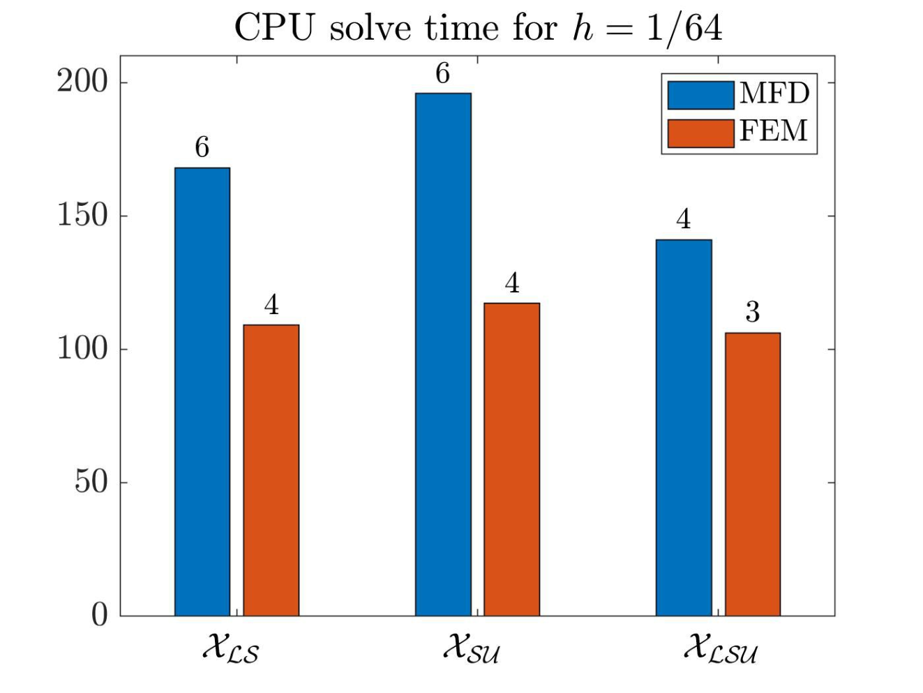
To further compare the two methods, CPU solve time per time iteration is examined for fixed time-step size, as well as the time scaling of the solve time per time step for the three preconditioned FGMRES solvers, both with respect to mesh refinement. In Table 4, the average solve time over ten iterations with fixed τ\tau is reported. We see that as the number of degrees of freedom increases, the FE method beats MFD, especially for 𝒳ℒ​𝒮\mathcal{X}_{\mathcal{LS}} and 𝒳𝒮​𝒰\mathcal{X}_{\mathcal{SU}}. This is further demonstrated in Figure 5, where a side-by-side comparison of the three preconditioners for MFD and FEM is given. This time disparity is likely given by the fact that MFD takes slightly more GMRES iterations per solve, which could be due to the fact that the MFD system is not symmetric while FEM is.

hh 14\frac{1}{4} 18\frac{1}{8} 116\frac{1}{16} 132\frac{1}{32} 164\frac{1}{64}
MFD 𝒳ℒ​𝒮\mathcal{X}_{\mathcal{LS}} 1.32×10−21.32\times 10^{-2} 1.06×10−11.06\times 10^{-1} 9.95×10−19.95\times 10^{-1} 1.31×1011.31\times 10^{1} 1.68×1021.68\times 10^{2}
𝒳𝒮​𝒰\mathcal{X}_{\mathcal{SU}} 1.48×10−21.48\times 10^{-2} 1.12×10−11.12\times 10^{-1} 1.10×1001.10\times 10^{0} 1.41×1011.41\times 10^{1} 1.96×1021.96\times 10^{2}
𝒳ℒ​𝒮​𝒰\mathcal{X}_{\mathcal{LSU}} 1.06×10−21.06\times 10^{-2} 8.32×10−28.32\times 10^{-2} 8.15×10−18.15\times 10^{-1} 1.12×1011.12\times 10^{1} 1.41×1021.41\times 10^{2}
FEM 𝒳ℒ​𝒮\mathcal{X}_{\mathcal{LS}} 2.05×10−22.05\times 10^{-2} 1.08×10−11.08\times 10^{-1} 8.84×10−18.84\times 10^{-1} 9.62×1009.62\times 10^{0} 1.09×1021.09\times 10^{2}
𝒳𝒮​𝒰\mathcal{X}_{\mathcal{SU}} 2.45×10−22.45\times 10^{-2} 1.24×10−11.24\times 10^{-1} 1.02×1001.02\times 10^{0} 1.19×1011.19\times 10^{1} 1.17×1021.17\times 10^{2}
𝒳ℒ​𝒮​𝒰\mathcal{X}_{\mathcal{LSU}} 1.79×10−21.79\times 10^{-2} 9.17×10−29.17\times 10^{-2} 7.57×10−17.57\times 10^{-1} 8.04×1008.04\times 10^{0} 1.06×1021.06\times 10^{2}
Table 4: Average CPU solve time per time iteration over ten time steps with τ=0.1\tau=0.1 for MFD and FEM with all preconditioners.
Refer to caption
Figure 5: Comparison of solve time averaged over ten time steps of τ=0.1\tau=0.1 for MFD and FEM for fixed mesh size h=164h=\frac{1}{64}. The number of FGMRES iterations is given above each bar.

Finally, it is expected that the solve time scales 𝒪⁡(N​log⁡(N))\mathcal{O}\left(N\log(N)\right), where NN is the number of degrees of freedom. Figure 6 verifies this, where both FE and MFD results follow the trend of the reference line for all three preconditioners.

Based on the results presented, we conclude that all three preconditioners are robust and effective for solving the MFD system, and give comparable results to the FE method. In terms of both solve time and iteration counts, 𝒳ℒ​𝒮​𝒰\mathcal{X}_{\mathcal{LSU}} is the best preconditioner for both methods, which was also concluded in [2] for the FE method.

Refer to caption
Refer to caption
Figure 6: Time scaling of solve time averaged over ten time steps of τ=0.1\tau=0.1 for FEM(left) and MFD(right), where NN is the number of degrees of freedom.

7 Conclusions

By examining MFD in a FE framework, we are able to exploit the FEM tools and theory to strengthen the MFD method for Maxwell. From this equivalence of the two methods, well-posedness of the MFD system is proven with Babuska-Brezzi theory. Numerical results demonstrate that the FE convergence theory is recoverable in the MFD implementation. Furthermore, in showing well-posedness of the Maxwell MFD discretization and the connection to the FEM, robust block preconditioners developed for the FEM in [2] are adopted for solving the MFD linear system efficiently. When using structure-preserving discretizations, the goal is to enforce the PDE constraints, particularly a divergence-free magnetic field for Maxwell’s equations, at all time steps and all solve iterations. The block preconditioners for GMRES developed here are shown to be robust and guarantee all properties of the discretization at each time step.

All of the results in this paper apply to lowest–order FE and MFD methods. While higher–order MFD methods exist [14, 21, 22], connections to higher–order FEM are unclear and require further investigation. If such relationships are found, the analysis presented here should be valid. Additionally, a priori error estimates for MFD for Maxwell could be derived in a fashion similar to the techniques used for Darcy flow in [13]. Furthermore, now that a FE framework for MFD has been developed for the full Maxwell system, other electromagnetic applications can be explored such as MHD, time-harmonic Maxwell, or 𝑯⁡(curl)\bm{H}(\operatorname{curl}) and 𝑯⁡(div)\bm{H}(\operatorname{div}) problems, in general. The structure-preserving nature of the MFD discretization opens the door for many more physical applications with PDE constraints to be explored.

Acknowledgments

The work of JHA and XH was partially funded by National Science Foundation grant DMS-1620063. The work of LTZ was supported in part by NSF DMS-1720114 and DMS-1819157.

References

  • [1] J. H. Adler, X. Hu, and L. T. Zikatanov, HAZmath: A simple finite element, graph, and solver library, 2014-2020. https://bitbucket.org/hazmath/hazmath/wiki/Home.
  • [2]  , Robust solvers for Maxwell’s equations with dissipative boundary conditions, SIAM J. Sci. Comput., 39 (2017), pp. S3–S23.
  • [3] J. H. Adler, V. Petkov, and L. T. Zikatanov, Numerical approximations of asymptotically disappearing solutions of Maxwell’s equations, SIAM J. Sci. Comput., 35 (2013), pp. S386–S401.
  • [4] D. N. Arnold, R. S. Falk, and R. Winther, Finite element exterior calculus, homological techniques, and applications, Acta Numer., 6 (2006), pp. 1–155.
  • [5] I. Babuška, The finite element method with Lagrangian multipliers, Numer. Math., 20 (1972/73), pp. 179–192.
  • [6] J. Baranger, J. F. Maitre, and F. Oudin, Application de la théorie des éléments finis mixtes à l’étude d’une classe de schémas aux volumes différences finis pour les problèmes elliptiques, C.R. Acad. ScL Paris, 319 (1994), pp. 401–404.
  • [7]  , Connection between finite volume and mixed finite element methods, Modélisation mathématique et analyse numérique, 30 (1996), pp. 445–465.
  • [8] L. Beirao da Veiga, K. Lipnikov, and G. Manzini, The mimetic finite difference method for elliptic problems, Springer, 2014, ch. 2,7.
  • [9] M. Benzi and G. H. Golub, Numerical solution of saddle point problems, Acta Numer., (2005), pp. 1–137.
  • [10]  , A preconditioner for generalized saddle point problems, SIAM J. Maxtrix Anal. Appl., (2005), pp. 20–41.
  • [11] V. A. Bokil, N. Gibson, V. Gyrya, and D. McGregor, Dispersion reducing methods for edge discretizations of the electric vector wave equation, J. Comput. Phys., 287 (2015), pp. 88–109.
  • [12] F. Brezzi, On the existence, uniqueness and approximation of saddle-point problems arising from Lagrangian multipliers, Rev. Française Automat. Informat. Recherche Opérationnelle Sér. Rouge, 8 (1974), pp. 129–151.
  • [13] F. Brezzi, M. Fortin, and L. D. Marini, Error analysis of piecewise constant pressure approximations of Darcy’s law, Comput. Methods Appl. Engrg., 195 (2006), pp. 1547–1559.
  • [14] J. Castillo, J. Hyman, M. Shashkov, and S. Steinberg, High-order mimetic finite difference methods on nonuniform grids, Houston J. Math, Special Issue (1995), pp. 347–361.
  • [15] C. Greif and D. Schotzau, Preconditioners for the discretized time-harmonic Maxwell equations in mixed form, Numer. Linear Algebra Appl., (2007), p. . 281–297.
  • [16] R. Hiptmair, Finite elements in computatational electromagnetism, Acta Numer., 11 (2002), pp. 237–339.
  • [17] R. Hiptmair and J. Xu, Nodal Auxiliary Space Preconditioning in H(curl) and H(div) Spaces, SIAM Journal on Numerical Analysis, 45 (2007), pp. 2483–2509.
  • [18] K. Hu, Y. Ma, and J. Xu, Stable finite element methods preserving ∇⁣⋅\nabla\cdotB=0 exactly for MHD models, Numerische Mathematik, 135 (2017), pp. 371–396.
  • [19] J. M. Hyman and M. Shashkov, Mimetic discretizations for Maxwell’s equations, J. Comput. Phys., (1999), pp. 881–909.
  • [20] T. V. Kolev and P. S. Vassilevski, Parallel auxiliary space AMG for H(curl) problems, Journal of Computational Mathematics, 27 (2009), pp. 604–623.
  • [21] K. Lipnikov and V. Gyrya, High-order mimetic finite difference method for diffusion problems on polygonal meshes, J. Comput. Phys., 227 (2008), pp. 8841–8854.
  • [22] K. Lipnikov, G. Manzini, and M. Shashkov, Mimetic finite difference method, J. Comput. Phys., (2013).
  • [23] D. Loghin and A. J. Wathen, Analysis of preconditioners for saddle point problems, SIAM J. Sci. Comput., (2004), pp. 2029–2049.
  • [24] Y. Ma, K. Hu, X. Hu, and J. Hu, Robust preconditioners for incompressible mhd models, J.Comput. Phys., (2016), pp. 721–749.
  • [25] K. A. Mardal and R. Winther, Preconditioning discretizations of systems of partial differential equations, Numer. Linear Algebra Appl., (2011), pp. 1–40.
  • [26] P. Monk, Finite element methods for Maxwell’s equations, Num. Math. Sci. Comput., Oxford University Press, New York, 2003.
  • [27] E. Phillips, J. Shadid, and E. Cyr, Scalable preconditioners for structure preserving discretizations of Maxwell equations in first order form, SIAM J. Sci. Comput., 4 (2018), pp. B723–B742.
  • [28] E. Phillips, J. Shadid, E. Cyr, H. Elman, and R. Pawlowski, Block preconditioners for stable mixed nodal and edge finite element representations of incompressible resistive MHD, SIAM J. Sci. Comput., 38 (2016), p. B1009–B1031.
  • [29] C. Rodrigo, F. J. Gaspar, X. Hu, and L. T. Zikatanov, Finite element framework for some mimetic finite difference discretizations, Comput. Math. Appl., 70 (2015), pp. 2661–2673.
  • [30] V. Thomée, Galerkin finite element methods for parabolic problem, Springer, 1997, ch. 15.
  • [31] P. N. Vabishchevich, Finite-difference approximation of mathematical physics problems on irregular grids, Comput. Methods in Appl. Math., 5 (2005), pp. 294–330.
  • [32] S.-L. Wu, T.-Z. Huang, and C.-X. Li, Modified block preconditioners for the discretized timeharmonic Maxwell equations in mixed form, J. Comput. Appl. Math., (2013), p. 419–431.