跳到论文正文
W Papers独立论文阅读器 arXiv:2012.02932 论文正文 计算阅读时间 · 0%
引用这篇论文根据当前论文元数据生成,正式投稿前建议核对。


License: arXiv.org perpetual non-exclusive license
arXiv:2012.02932v1 [math.DS] 05 Dec 2020

On Periodical Damping Ratio of a Controlled Dynamical System with Parametric Resonances

Xin Xu    Kai Sun    Thanks: X. Xu and K. Sun are with the Department of Electrical and Computer Engineering, the University of Tennessee, Knoxville, TN, 37919. Thanks:  E-mail: xxu30@vols.utk.edu, kaisun@utk.edu
Abstract

This report provides an interpretation on the periodically varying damping ratio of a dynamical system with direct control of oscillation or vibration damping. The principal parametric resonance of the system and a new type of parametric resonance, named ”zero-th order” parametric resonance, are investigated by using the method of multiple scales to find approximate, analytical solutions of the system, which provide an interpretation on such damping variations.

Keywords - Method of multiple scales, damping, parametric resonance.

I Introduction

This study is motivated by the direct control of oscillation or vibration damping with a weakly-damped dynamical system. The dynamics regarding a specific mode can be approximated by a one-degree-of-freedom (1-DOF) system having a direct damping improvement as modeled by (1):

x¨+(−2​σ+u)​x˙+(σ2+ω2)​x=0\ddot{x}+(-2\sigma+u)\dot{x}+(\sigma^{2}+\omega^{2})x=0 (1)

where xx is a state. Parameter uu is the increased damping by, e.g., a feedback controller that measures real-time damping ratio and eliminates its error from a reference damping ratio. If u=0u=0, the eigenvalue λ\lambda is calculated by (2), where ζ\zeta and wnw_{n} are the damping ratio and natural angular frequency, respectively.

λ1,2=σ±j​ω=−ζ​ωn±j​ωn​1−ζ2\lambda_{1,2}=\sigma\pm j\omega=-\zeta\omega_{n}\pm j\omega_{n}\sqrt{1-\zeta^{2}} (2)

Considering the dynamics of uu over time, approximate uu by a periodic function K​c​o​s​(Ω​t)Kcos(\Omega t), where KK and Ω\Omega are its amplitude and angular frequency, respectively. Eq. (1) becomes (3). By using the method of multiple scales (MMS), it will be shown that a) the principal parametric resonance can be excited when Ω≈2​ω\Omega\approx 2\omega and b), the “zero-th order” parametric resonance will be excited when Ω≈0\Omega\approx 0, which is why it is called “zero-th order”.

x¨+(−2​σ+K​c​o​s​(Ω​t))​x˙+(σ2+ω2)​x=0\ddot{x}+(-2\sigma+Kcos(\Omega t))\dot{x}+(\sigma^{2}+\omega^{2})x=0 (3)

In the rest of the report, principal and ”zero-th order” parametric resonances of the system are respectively investigated in sections II and III, and conclusions are drawn in section IV.

II Principal Parametric Resonance

When Ω≈2​ω\Omega\approx 2\omega, the principal parametric resonance can be observed in the response of xx. For instance, let ζ\zeta = 0.0098, ωn\omega_{n} = 3.8072 rad/s, KK = 0.5, and consequently, σ\sigma = 0.0373 and ω\omega = 3.8070 rad/s. Then, if let Ω\Omega = 6.9115 rad/s and let the initial value be x=1,x˙=0x=1,\dot{x}=0, the response of xx is shown in Fig. 1 with its envelop being marked and the damping ratio estimated, e.g., from Prony’s method is given in Fig. 2. The periodic variation in the measured damping ratio shows the parametric resonance due to Ω≈2​ω\Omega\approx 2\omega.

Refer to caption
Fig. 1: Principal parametric resonance: response of xx.
Refer to caption
Fig. 2: Principal parametric resonance: measured damping ratio.

The parametric resonance can be investigated by finding an asymptotic solution via the MMS for (3), through which some properties could be revealed. The basic idea of MMS is to find an asymptotic solution of a perturbed system considering different time scales. The use of MMS follows the methodology in [1, 2], and [3]. First, the periodic parameter K​c​o​s​(Ω​t)Kcos(\Omega t) is treated as a perturbation by inserting a small dimensionless parameter ε>0\varepsilon>0 like in (4), where Kε=K/εK_{\varepsilon}=K/\varepsilon.

x¨+(−2​σ+ε​Kε​c​o​s​(Ω​t))​x˙+(σ2+ω2)​x=0\ddot{x}+(-2\sigma+\varepsilon K_{\varepsilon}cos(\Omega t))\dot{x}+(\sigma^{2}+\omega^{2})x=0 (4)

Then, a first order uniform solution of (4) is sought in the form of (5):

x⁡(ε,T0,T1)≈x0​(T0,T1)+ε​x1​(T0,T1)T0=t,T1=ε​t\begin{matrix}x(\varepsilon,T_{0},T_{1})\approx x_{0}(T_{0},T_{1})+\varepsilon x_{1}(T_{0},T_{1})\\ T_{0}=t,T_{1}=\varepsilon t\end{matrix} (5)

where T1T_{1} is introduced as a slow-scale time variable, such that (5) could consider the evolution of the solution over long time-scales of the order ε−1\varepsilon^{-1}. Note that x0x_{0} is exactly the solution of (4) when ε\varepsilon = 0, and x1x_{1} is the part caused by the perturbation. Substitute (5) into (4) and equate the coefficients of powers of ε\varepsilon:

D02​x0−2​σ​D0​x0+(σ2+ω2)​x0=0D_{0}^{2}x_{0}-2\sigma D_{0}x_{0}+(\sigma^{2}+\omega^{2})x_{0}=0 (6)
D02​x1−2​σ​D0​x1+(σ2+ω2)​x1=−2​D1​D0​x0−Kε​c​o​s​(Ω​T0)​D0​x0+2​σ​D1​x0D_{0}^{2}x_{1}-2\sigma D_{0}x_{1}+(\sigma^{2}+\omega^{2})x_{1}=-2D_{1}D_{0}x_{0}-K_{\varepsilon}cos(\Omega T_{0})D_{0}x_{0}+2\sigma D_{1}x_{0} (7)

where Dn=∂/∂TnD_{n}=\partial/\partial T_{n}.

The solution of (6) can be expressed in a complex form:

x0​(T0,T1)=A⁡(T1)​e(σ+j​ω)​T0+A¯​(T1)​e(σ−j​ω)​T0x_{0}(T_{0},T_{1})=A(T_{1})e^{(\sigma+j\omega)T_{0}}+\bar{A}(T_{1})e^{(\sigma-j\omega)T_{0}} (8)

where the bar denotes the complex conjugate. Substitute (8) into (7):

D02​x1−2​σ​D0​x1+(σ2+ω2)​x1=\displaystyle D_{0}^{2}x_{1}-2\sigma D_{0}x_{1}+(\sigma^{2}+\omega^{2})x_{1}= −2​(σ+j​ω)​e(σ+j​ω)​T0​D1​A−2​ζ​ωn​e(σ+j​ω)​T0​D1​A\displaystyle-2(\sigma+j\omega)e^{(\sigma+j\omega)T_{0}}D_{1}A-2\zeta\omega_{n}e^{(\sigma+j\omega)T_{0}}D_{1}A (9)
−Kε2​[(σ+j​ω)​e(σ+j⁡(Ω+ω))​T0​A+(σ−j​ω)​e(σ+j⁡(Ω−ω))​T0​A¯]+C.C.\displaystyle-\frac{K_{\varepsilon}}{2}\left[(\sigma+j\omega)e^{(\sigma+j(\Omega+\omega))T_{0}}A+(\sigma-j\omega)e^{(\sigma+j(\Omega-\omega))T_{0}}\bar{A}\right]+C.C.

where C.C.C.C. denotes the complex conjugates of the former two terms. Introduce a detuning parameter ξ\xi such that Ω=2​ω+ε​ξ\Omega=2\omega+\varepsilon\xi, (9) can be converted to:

D02​x1−2​σ​D0​x1+(σ2+ω2)​x1=\displaystyle D_{0}^{2}x_{1}-2\sigma D_{0}x_{1}+(\sigma^{2}+\omega^{2})x_{1}= −[2​(σ+j​ω)​D1​A−2​σ​D1​A+Kε2​(σ−j​ω)​ej​ε​ξ​T0​A¯]​e(σ+j​ω)​T0\displaystyle-\left[2(\sigma+j\omega)D_{1}A-2\sigma D_{1}A+\frac{K_{\varepsilon}}{2}(\sigma-j\omega)e^{j\varepsilon\xi T_{0}}\bar{A}\right]e^{(\sigma+j\omega)T_{0}} (10)
−Kε2​(σ+j​ω)​e(σ+j⁡(Ω+ω))​T0​A+C.C.\displaystyle-\frac{K_{\varepsilon}}{2}(\sigma+j\omega)e^{(\sigma+j(\Omega+\omega))T_{0}}A+C.C.

It can be verified that the condition (11) should be met to avoid generating secular terms in the solution of xx. The explanation of secular term can be found in [3]. In this problem it will be a term grows linearly in tt, such that the identified solution will be unbounded, while in fact the true solution is bounded.

2​(σ+j​ω)​D1​A−2​σ​D1​A+Kε2​(σ−j​ω)​ej​ε​ξ​T0​A¯=02(\sigma+j\omega)D_{1}A-2\sigma D_{1}A+\frac{K_{\varepsilon}}{2}(\sigma-j\omega)e^{j\varepsilon\xi T_{0}}\bar{A}=0 (11)

With the condition (11), the solution of (10) is given below.

x1​(T0,T1)=Kε​(σ+j​ω)​A2​(e(σ+j⁡(Ω+ω))​T0Ω⁡(Ω+2​ω)+e(σ−j​ω)​T02​ω​(Ω+2​ω)−e(σ+j​ω)​T02​ω​Ω)+C.C.x_{1}(T_{0},T_{1})=\frac{K_{\varepsilon}(\sigma+j\omega)A}{2}\left(\frac{e^{(\sigma+j(\Omega+\omega))T_{0}}}{\Omega(\Omega+2\omega)}+\frac{e^{(\sigma-j\omega)T_{0}}}{2\omega(\Omega+2\omega)}-\frac{e^{(\sigma+j\omega)T_{0}}}{2\omega\Omega}\right)+C.C. (12)

x1x_{1} could be ignored compared to x0x_{0}, since usually it is numerically small. Hence, assume x​(t)≈x0​(t)x(t)\approx x_{0}(t). A⁡(T1)A(T_{1}) can be determined by solving (11). For a weakly-damped system, σ\sigma can be assumed to be zero and (11) can be converted to:

d​Ad​T1=Kε4​ej​ξ​T1​A¯\frac{dA}{dT_{1}}=\frac{K_{\varepsilon}}{4}e^{j\xi T_{1}}\bar{A} (13)

The analytical solutions of A⁡(T1)A(T_{1}) and x⁡(t)x(t) can be found for three cases, 1) (Ω−2​ω)2−K2/4>0(\Omega-2\omega)^{2}-K^{2}/4>0, 2) (Ω−2​ω)2−K2/4<0(\Omega-2\omega)^{2}-K^{2}/4<0, and 3) (Ω−2​ω)2−K2/4=0(\Omega-2\omega)^{2}-K^{2}/4=0. For the sake of convenience, define ωK=|ξ2−Kε2/4|=|(Ω−2​ω)2−K2/4|/ε\omega_{K}=\sqrt{|\xi^{2}-K_{\varepsilon}^{2}/4|}=\sqrt{|(\Omega-2\omega)^{2}-K^{2}/4|}/\varepsilon, and let A0=Ar​e​0+j​Ai​m​0A_{0}=A_{re0}+jA_{im0} be the given initial value of A⁡(T1)A(T_{1}).

II-A Case 1: (Ω−2​ω)2−K2/4>0(\Omega-2\omega)^{2}-K^{2}/4>0

The solution of A⁡(T1)A(T_{1}) is:

A⁡(T1)=(C1​ej⁡(r1−ωK​T1)+C2​ej​r2)​ej​ξ+ωK2​T1A(T_{1})=(C_{1}e^{j(r_{1}-\omega_{K}T_{1})}+C_{2}e^{jr_{2}})e^{j\frac{\xi+\omega_{K}}{2}T_{1}} (14)
{C1=ξ+ωK2​ωK2​ξ⁡(Ar​e​02+Ai​m​02)+Kε​Ar​e​0​Ai​m​0C2=ξ−ωK2​ωK2​ξ⁡(Ar​e​02+Ai​m​02)+Kε​Ar​e​0​Ai​m​0r1=a​r​c​t​a​n​(2​Ai​m​0​(ξ+ωK)+Kε​Ar​e​02​Ar​e​0​(ξ+ωK)+Kε​Ai​m​0)r2=a​r​c​t​a​n​(2​Ai​m​0​(ξ−ωK)+Kε​Ar​e​02​Ar​e​0​(ξ−ωK)+Kε​Ai​m​0)\left\{\begin{aligned} C_{1}&=\sqrt{\frac{\xi+\omega_{K}}{2\omega_{K}^{2}}}\sqrt{\xi(A_{re0}^{2}+A_{im0}^{2})+K_{\varepsilon}A_{re0}A_{im0}}\\ C_{2}&=\sqrt{\frac{\xi-\omega_{K}}{2\omega_{K}^{2}}}\sqrt{\xi(A_{re0}^{2}+A_{im0}^{2})+K_{\varepsilon}A_{re0}A_{im0}}\\ r_{1}&=arctan\left(\frac{2A_{im0}(\xi+\omega_{K})+K_{\varepsilon}A_{re0}}{2A_{re0}(\xi+\omega_{K})+K_{\varepsilon}A_{im0}}\right)\\ r_{2}&=arctan\left(\frac{2A_{im0}(\xi-\omega_{K})+K_{\varepsilon}A_{re0}}{2A_{re0}(\xi-\omega_{K})+K_{\varepsilon}A_{im0}}\right)\end{aligned}\right. (15)

The solution of x⁡(t)x(t) is obtained by substituting (14) into (5) and ignoring x1x_{1}:

x⁡(t)=2​C1​eσ​t​c​o​s​(ωC​t+r1−ε​ωK​t)+2​C2​eσ​t​c​o​s​(ωC​t+r2)x(t)=2C_{1}e^{\sigma t}cos(\omega_{C}t+r_{1}-\varepsilon\omega_{K}t)+2C_{2}e^{\sigma t}cos(\omega_{C}t+r_{2}) (16)
ωC=ω+ξ+ωK2​ε\omega_{C}=\omega+\frac{\xi+\omega_{K}}{2}\varepsilon (17)

At the first glance, x⁡(t)x(t) seems to depend on ε\varepsilon and ξ\xi. Actually, such dependence can be immediately removed by substituting ξ=(Ω−2​ω)/ε\xi=(\Omega-2\omega)/\varepsilon, ωK=|(Ω−2​ω)2−K2/4|/ε\omega_{K}=\sqrt{|(\Omega-2\omega)^{2}-K^{2}/4|}/\varepsilon, (15) and (17) into (16). The final expression is not given here for the sake of brevity.

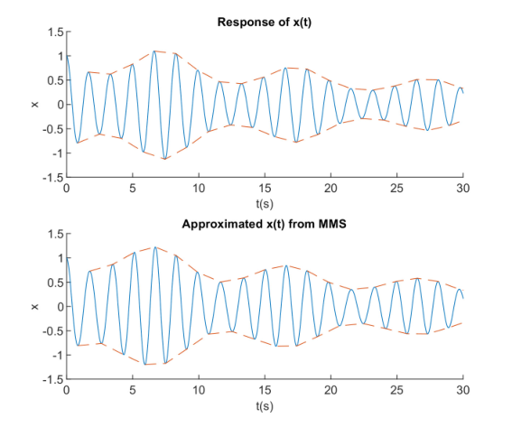
The resulting x⁡(t)x(t) consists of two components. The magnitude of the first component is 2​C12C_{1} and the frequency is ωC−ε​ωK\omega_{C}-\varepsilon\omega_{K}. The magnitude of the second component is 2​C22C_{2} and the frequency is ωC\omega_{C}. The validity of the approximated solution can be visualized by the case when Ω\Omega = 6.9115 rad/s. The comparison of the true response of x⁡(t)x(t) and the approximated x⁡(t)x(t) from (16) is shown in Fig. 3. The approximated x⁡(t)x(t) is almost the same as the true response.

Refer to caption
Fig. 3: Comparison of true response and approximated solution: (Ω−2​ω)2−K2/4>0(\Omega-2\omega)^{2}-K^{2}/4>0.

The principal parametric resonance in this case can be interpreted as follows. Without loss of generality, only consider the case when C2C_{2} is larger than C1C_{1}. The second component can be more dominant than the first component. Since ε​ωK\varepsilon\omega_{K} is much smaller than ωC\omega_{C}, the term ε​ωK​t\varepsilon\omega_{K}t can be viewed as a slow change of phase of the first component. Then, the change of damping of x⁡(t)x(t) can be interpreted as the periodically phase shift between the two components. When r1−εωKt≈r2+2mπ,m=0,±1,±2,…r_{1}-\varepsilon\omega_{K}t\approx r_{2}+2m\pi,m=0,\pm 1,\pm 2,..., the two components are in-phase and the magnitude of x⁡(t)x(t) is amplified. When r1−εωKt≈r2+2mπ+π,m=0,±1,±2,…r_{1}-\varepsilon\omega_{K}t\approx r_{2}+2m\pi+\pi,m=0,\pm 1,\pm 2,..., the two components are out-of-phase and the magnitude of x⁡(t)x(t) is reduced. This change is periodical at a frequency equal to ε​ωK=(Ω−2​ω)2−K2/4\varepsilon\omega_{K}=\sqrt{(\Omega-2\omega)^{2}-K^{2}/4}, and it makes the response of x⁡(t)x(t) to exhibit a periodically varying damping.

II-B Case 2: (Ω−2​ω)2−K2/4<0(\Omega-2\omega)^{2}-K^{2}/4<0

The solution of A⁡(T1)A(T_{1}) is:

A⁡(T1)=(C3​ej​r3+C4​ej⁡(r4−ωK​T1))​ej​ξ+ωK2​T1A(T_{1})=(C_{3}e^{jr_{3}}+C_{4}e^{j(r_{4}-\omega_{K}T_{1})})e^{j\frac{\xi+\omega_{K}}{2}T_{1}} (18)
{C3=Kε​(2​Kε+ωK)ωK2​|Ar​e​0+Ai​m​0​2​ξKε+2​ωK|C4=Kε​(2​Kε−ωK)ωK2​|Ar​e​0+Ai​m​0​2​ξKε−2​ωK|r3=a​r​c​t​a​n​(−Ai​m​0​(Kε−2​ωK)−2​ξ​Ar​e​0Ar​e​0​(Kε+2​ωK)+2​ξ​Ai​m​0)r4=a​r​c​t​a​n​(Ai​m​0​(Kε+2​ωK)+2​ξ​Ar​e​0−Ar​e​0​(Kε−2​ωK)−2​ξ​Ai​m​0)\left\{\begin{aligned} C_{3}&=\sqrt{\frac{K_{\varepsilon}(2K_{\varepsilon}+\omega_{K})}{\omega_{K}^{2}}}\left|A_{re0}+A_{im0}\frac{2\xi}{K_{\varepsilon}+2\omega_{K}}\right|\\ C_{4}&=\sqrt{\frac{K_{\varepsilon}(2K_{\varepsilon}-\omega_{K})}{\omega_{K}^{2}}}\left|A_{re0}+A_{im0}\frac{2\xi}{K_{\varepsilon}-2\omega_{K}}\right|\\ \\ r_{3}&=arctan\left(\frac{-A_{im0}(K_{\varepsilon}-2\omega_{K})-2\xi A_{re0}}{A_{re0}(K_{\varepsilon}+2\omega_{K})+2\xi A_{im0}}\right)\\ r_{4}&=arctan\left(\frac{A_{im0}(K_{\varepsilon}+2\omega_{K})+2\xi A_{re0}}{-A_{re0}(K_{\varepsilon}-2\omega_{K})-2\xi A_{im0}}\right)\\ \end{aligned}\right. (19)

The solution of x⁡(t)x(t) is obtained by substituting (18) into (5) and ignoring x1x_{1}. Similarly to (16), the solution (20) also does not depend on ε\varepsilon and ξ\xi.

x⁡(t)=2​C3​e(σ+ε​ωK2)​t​c​o​s​((ω+Ω2)​t+r3)+2​C4​e(σ−ε​ωK2)​t​c​o​s​((ω+Ω2)​t+r4)x(t)=2C_{3}e^{(\sigma+\varepsilon\frac{\omega_{K}}{2})t}cos\left((\omega+\frac{\Omega}{2})t+r_{3}\right)+2C_{4}e^{(\sigma-\varepsilon\frac{\omega_{K}}{2})t}cos\left((\omega+\frac{\Omega}{2})t+r_{4}\right) (20)

The resulting x⁡(t)x(t) consists of two components. The magnitude of the first component is 2​C32C_{3} and the magnitude of the second component is 2​C42C_{4}. The frequency of both components is ω+Ω/2\omega+\Omega/2. The two components of x⁡(t)x(t) have damping coefficient different from σ\sigma. This validity of the approximated solution can be verified by the case when Ω\Omega is changed to 7.5524 rad/s. The comparison of the true response of x⁡(t)x(t) and the approximated x⁡(t)x(t) from (20) is shown in Fig. 4. The approximated x⁡(t)x(t) is almost the same as the true response. Note that the response diverges since the damping part of the first component becomes positive.

Refer to caption
Fig. 4: Comparison of true response and approximated solution: (Ω−2​ω)2−K2/4<0(\Omega-2\omega)^{2}-K^{2}/4<0.

In this case, the response of x⁡(t)x(t) will not exhibit a periodically varying damping, but might exhibit a time-variant damping. If C3C_{3} is much larger than C4C_{4}, the first component will be dominant at the early stage and the response of x⁡(t)x(t) will be damped in a fast pace. Then, the first component will take the dominance after the second component is damped out.

II-C Case 3: (Ω−2​ω)2−K2/4<0(\Omega-2\omega)^{2}-K^{2}/4<0

The solution of A⁡(T1)A(T_{1}) is:

A⁡(T1)=A0​ej​Kε4​T1+Kε4​(A¯0−j​A0)​T1​ej​Kε4​T1,i​fΩ−2​ω=K2A⁡(T1)=A0​e−j​Kε4​T1−Kε4​(A¯0−j​A0)​T1​e−j​Kε4​T1,i​fΩ−2​ω=−K2\begin{matrix}A(T_{1})=A_{0}e^{j\frac{K_{\varepsilon}}{4}T_{1}}+\frac{K_{\varepsilon}}{4}(\bar{A}_{0}-jA_{0})T_{1}e^{j\frac{K_{\varepsilon}}{4}T_{1}},&if&\Omega-2\omega=\frac{K}{2}\\ A(T_{1})=A_{0}e^{-j\frac{K_{\varepsilon}}{4}T_{1}}-\frac{K_{\varepsilon}}{4}(\bar{A}_{0}-jA_{0})T_{1}e^{-j\frac{K_{\varepsilon}}{4}T_{1}},&if&\Omega-2\omega=-\frac{K}{2}\end{matrix} (21)

The solution of x⁡(t)x(t) is obtained by substituting (21) into (5) and ignoring x1x_{1}:

x⁡(t)=2​eσ​t​[(Ar​e​0+K4​(Ar​e​0+Ai​m​0)​t)​c​o​s​(Ω2​t)−(Ai​m​0−K4​(Ar​e​0+Ai​m​0)​t)​s​i​n​(Ω2​t)],i​fΩ−2​ω=K2x⁡(t)=2​eσ​t​[(Ar​e​0−K4​(Ar​e​0+Ai​m​0)​t)​c​o​s​(Ω2​t)−(Ai​m​0+K4​(Ar​e​0+Ai​m​0)​t)​s​i​n​(Ω2​t)],i​fΩ−2​ω=−K2\begin{matrix}x(t)=2e^{\sigma t}\left[\left(A_{re0}+\frac{K}{4}(A_{re0}+A_{im0})t\right)cos\left(\frac{\Omega}{2}t\right)-\left(A_{im0}-\frac{K}{4}(A_{re0}+A_{im0})t\right)sin\left(\frac{\Omega}{2}t\right)\right],&if&\Omega-2\omega=\frac{K}{2}\\ x(t)=2e^{\sigma t}\left[\left(A_{re0}-\frac{K}{4}(A_{re0}+A_{im0})t\right)cos\left(\frac{\Omega}{2}t\right)-\left(A_{im0}+\frac{K}{4}(A_{re0}+A_{im0})t\right)sin\left(\frac{\Omega}{2}t\right)\right],&if&\Omega-2\omega=-\frac{K}{2}\end{matrix} (22)

Each of the resulting x⁡(t)x(t) consists of two components at the frequency Ω/2\Omega/2. Note part of the results depends on tt, which may cause a time-variant damping.

This validity of the approximated solution can be verified by the case when Ω\Omega is changed to 7.3639 rad/s. The comparison of the true response of x⁡(t)x(t) and the approximated x⁡(t)x(t) from (22) is shown in Fig. 5. The approximated x⁡(t)x(t) is almost the same as the true response.

Refer to caption
Fig. 5: Comparison of true response and approximated solution: (Ω−2​ω)2−K2/4=0(\Omega-2\omega)^{2}-K^{2}/4=0.

Since the condition (Ω−2​ω)2−K2/4=0(\Omega-2\omega)^{2}-K^{2}/4=0 can hardly be met, this case is usually ignored in industrial applications.

III “Zero-th Order” Parametric Resonance

When Ω≈0\Omega\approx 0, the parametric resonance can also be observed in the response of xx, which is named as “zero-th order” parametric resonance here. For instance, let ζ\zeta = 0.0098, ωn\omega_{n} = 3.8072 rad/s, KK = 0.5, and consequently, σ\sigma = 0.0373 and ω\omega = 3.8070 rad/s. Then, if let Ω\Omega = 0.6283 rad/s and let the initial value be x=1,x˙=0x=1,\dot{x}=0, the response is shown in Fig. 6 with the envelop being marked and the measured damping ratio from the Prony’s method is given in Fig. 7. The periodic variation in the measured damping ratio shows the parametric resonance due to Ω≈0\Omega\approx 0.

Refer to caption
Fig. 6: “Zero-th order” parametric resonance: response of xx.
Refer to caption
Fig. 7: “Zero-th order” parametric resonance: measured damping ratio.

Through MMS, some properties of such a resonance is revealed. Again, consider a small dimensionless parameter ε\varepsilon as in (4), and take the same derivation as from (4) to (9). By introducing a detuning parameter ξ\xi such that Ω=ε​ξ\Omega=\varepsilon\xi, (9) can be converted to (23).

D02​x1−2​σ​D0​x1+(σ2+ω2)​x1=\displaystyle D_{0}^{2}x_{1}-2\sigma D_{0}x_{1}+(\sigma^{2}+\omega^{2})x_{1}= −[2​(σ+j​ω)​D1​A−2​σ​D1​A+Kε2​(σ+j​ω)​ej​ε​ξ​T0​A]​e(σ+j​ω)​T0\displaystyle-\left[2(\sigma+j\omega)D_{1}A-2\sigma D_{1}A+\frac{K_{\varepsilon}}{2}(\sigma+j\omega)e^{j\varepsilon\xi T_{0}}A\right]e^{(\sigma+j\omega)T_{0}} (23)
−Kε2​(σ−j​ω)​e(σ+j⁡(ε​ξ+ω))​T0​A¯+C.C.\displaystyle-\frac{K_{\varepsilon}}{2}(\sigma-j\omega)e^{(\sigma+j(\varepsilon\xi+\omega))T_{0}}\bar{A}+C.C.

It can be verified that the condition (24) should be met to avoid generating secular terms in the solution of x⁡(t)x(t).

2​(σ+j​ω)​D1​A−2​σ​D1​A+Kε2​(σ+j​ω)​ej​ε​ξ​T0​A=02(\sigma+j\omega)D_{1}A-2\sigma D_{1}A+\frac{K_{\varepsilon}}{2}(\sigma+j\omega)e^{j\varepsilon\xi T_{0}}A=0 (24)

Then, the solution of (23) is given below.

x1​(T0,T1)=Kε​(σ−j​ω)​A¯2​(e(σ+j⁡(Ω−ω))​T0Ω⁡(Ω−2​ω)+e(σ−j​ω)​T02​ω​Ω−e(σ+j​ω)​T02​ω​(2​ω−Ω))+C.C.x_{1}(T_{0},T_{1})=\frac{K_{\varepsilon}(\sigma-j\omega)\bar{A}}{2}\left(\frac{e^{(\sigma+j(\Omega-\omega))T_{0}}}{\Omega(\Omega-2\omega)}+\frac{e^{(\sigma-j\omega)T_{0}}}{2\omega\Omega}-\frac{e^{(\sigma+j\omega)T_{0}}}{2\omega(2\omega-\Omega)}\right)+C.C. (25)

x1x_{1} could be ignored compared to x0x_{0}, since usually it is numerically small. Hence, assume x​(t)≈x0​(t)x(t)\approx x_{0}(t). A⁡(T1)A(T_{1}) can be determined by solving (24). First convert (24) to (26). Then, the analytical solution of A⁡(T1)A(T_{1}) is shown in (27), where A0=Ar​e​0+j​Ai​m​0A_{0}=A_{re0}+jA_{im0} is the initial value of A⁡(T1)A(T_{1}).

d​Ad​T1=Kε​(−ω+j​σ)4​ω​ej​ξ​T1​A\frac{dA}{dT_{1}}=\frac{K_{\varepsilon}(-\omega+j\sigma)}{4\omega}e^{j\xi T_{1}}A (26)
A⁡(T1)=eKε​(σ+j​ω)4​ξ​ω​ej​ξ​T1+A0−eKε​(σ+j​ω)4​ξ​ωA(T_{1})=e^{\frac{K_{\varepsilon}(\sigma+j\omega)}{4\xi\omega}e^{j\xi T_{1}}}+A_{0}-e^{\frac{K_{\varepsilon}(\sigma+j\omega)}{4\xi\omega}} (27)

Substitute (27) into (5) and ignore x1x_{1}:

x⁡(t)\displaystyle x(t) =2​eK​σ2+ω24​Ω​ω​c​o​s​(Ω​t+θ)+σ​t​c​o​s​(K​σ2+ω24​Ω​ω​s​i​n​(Ω​t+θ)+ω​t)\displaystyle=2e^{\frac{K\sqrt{\sigma^{2}+\omega^{2}}}{4\Omega\omega}cos(\Omega t+\theta)+\sigma t}cos\left(\frac{K\sqrt{\sigma^{2}+\omega^{2}}}{4\Omega\omega}sin(\Omega t+\theta)+\omega t\right) (28)
+2​eσ​t​(Ar​e​0​c​o​s​(ω​t)−Ai​m​0​s​i​n​(ω​t)−eK​σ4​ω​Ω​c​o​s​(ω​t+K4​Ω))\displaystyle+2e^{\sigma t}\left(A_{re0}cos(\omega t)-A_{im0}sin(\omega t)-e^{\frac{K\sigma}{4\omega\Omega}}cos(\omega t+\frac{K}{4\Omega})\right)
θ=a​r​c​t​a​n​(ωσ)\theta=arctan\left(\frac{\omega}{\sigma}\right) (29)

The solution includes two components. Note that the first component has a periodically varying parameter c​o​s​(Ω​t+θ)cos(\Omega t+\theta) being added to the original damping part σ​t\sigma t, which could lead to a periodically varying damping in the response of x⁡(t)x(t). The s​i​n​(Ω​t+θ)sin(\Omega t+\theta) term in the first component can be viewed as a periodically varying phase of frequency Ω\Omega that leads to a periodic phase shift relative to the second component. Hence, the solution x⁡(t)x(t) will exhibit periodically varying damping ratio, and the frequency is close to Ω\Omega.

The validity of the approximated solution can be verified by the case when Ω\Omega is changed to 0.6283 rad/s. The comparison of the true response of x⁡(t)x(t) and the approximated x⁡(t)x(t) from (28) is shown in Fig. 8. The approximated x⁡(t)x(t) is almost the same as the true response.

Refer to caption
Fig. 8: Comparison of true response and approximated solution: “zero-th order” parametric resonance.

IV Conclusion

The response of a weakly-damped 1-DOF system with direct control of its damping ratio can exhibit parametric resonances under principal parametric excitation and “zero-th order” parametric excitation. It is shown that the principal parametric resonance can be classified into three cases depending on (Ω−2​ω)2−K2/4>0,<0(\Omega-2\omega)^{2}-K^{2}/4>0,<0, or =0=0. Specifically, when (Ω−2​ω)2−K2/4>0(\Omega-2\omega)^{2}-K^{2}/4>0, the magnitude of xx periodically variation in time at a frequency close to (Ω−2​ω)2−K2/4\sqrt{(\Omega-2\omega)^{2}-K^{2}/4}, which manifests periodical changes of its damping ratio. When “zero-th order” parametric resonance is excited, the magnitude of x⁡(t)x(t) can periodically vary in time at a frequency close to Ω\Omega.

References

  • [1] L. D. Zavodney, A. H. Nayfeh,“The response of a single-degree-of-freedom system with quadratic and cubic non-linearities to a fundamental parametric resonance,” Journal of Sound and Vibration, vol. 120, no. 1, pp. 63-93, 1988.
  • [2] L. D. Zavodney, A. H. Nayfeh, N. E. Sanchez,“The response of a single-degree-of-freedom system with quadratic and cubic non-linearities to a principal parametric resonance,” Journal of Sound and Vibration, vol. 129, no. 3, pp. 417-442, 1989.
  • [3] J. K. Kevorkian, J. D. Cole, Multiple scale and singular perturbation methods. Springer Science & Business Media, 2012.