Optimal local approximation spaces for parabolic problemsThanks: The work of Julia Schleuß was funded by the Deutsche Forschungsgemeinschaft (DFG, German Research Foundation) under Germany’s Excellence Strategy EXC 2044-390685587, Mathematics Münster: Dynamics-Geometry-Structure.
Abstract.
We propose local space-time approximation spaces for parabolic problems that are optimal in the sense of Kolmogorov and may be employed in multiscale and domain decomposition methods. The diffusion coefficient can be arbitrarily rough in space and time. To construct local approximation spaces we consider a compact transfer operator that acts on the space of local solutions and covers the full time dimension. The optimal local spaces are then given by the left singular vectors of the transfer operator. To prove compactness of the latter we combine a suitable parabolic Caccioppoli inequality with the compactness theorem of Aubin-Lions. In contrast to the elliptic setting [I. Babuška and R. Lipton, Multiscale Model. Simul., 9 (2011), pp. 373-406] we need an additional regularity result to combine the two results. Furthermore, we employ the generalized finite element method to couple local spaces and construct an approximation of the global solution. Since our approach yields reduced space-time bases, the computation of the global approximation does not require a time stepping method and is thus computationally efficient. Moreover, we derive rigorous local and global a priori error bounds. In detail, we bound the global approximation error in a graph norm by the local errors in the -norm, noting that the space the transfer operator maps to is equipped with this norm. Numerical experiments demonstrate an exponential decay of the singular values of the transfer operator and the local and global approximation errors for problems with high contrast or multiscale structure regarding space and time.
Key words and phrases:
multiscale methods, parabolic problems, space-time Petrov-Galerkin methods, Kolmogorov n-width, a priori error bound, generalized finite element method2010 Mathematics Subject Classification
65M12, 65M15, 65M55, 65M601. Introduction
In certain industrial applications and environmental sciences, modeling and simulating phenomena such as the transport of pollutants in the groundwater is of great interest. These problems exhibit highly varying and heterogeneous multiscale features since both local fine-scale effects such as capillary pressures and the coarse-scale flow behavior have a significant influence on the overall concentration and distribution of the pollutant. In addition, the respective coefficient functions can be rough in space and time. Therefore, a numerical simulation using standard techniques such as the finite element (FE) or the finite volume method can be prohibitively expensive. In fact, the FE method based on classical polynomials can perform arbitrarily bad for heterogeneous problems with rough coefficients [5]. Well-known strategies to address these problems are domain decomposition [30, 37, 45, 68] and multiscale methods [8, 24, 25, 28, 33, 38, 39, 53, 55, 58, 59, 60]. The latter are based on ansatz functions which incorporate the local behavior of the (numerical) solution of the PDE.
Localizable multiscale methods that allow controlling both the error due to localization and the global approximation error at a certain rate, but do not rely on structural assumptions such as periodicity or scale separation, have been developed in the last decade. So far, such type of multiscale methods have been proposed for problems with coefficients that are rough in space and include optimal local approximation spaces [8, 19, 25], localized bases based on the flux transfer property [58], adaptive local finite elements (AL basis) [33], the local orthogonal decomposition [52, 53], rough polyharmonic splines [60], and gamblets [59].
In this paper, we propose optimal local approximation spaces, and, to the best of our knowledge, for the first time such type of multiscale methods for parabolic problems with coefficients that are rough in both space and time. We conjecture that the concepts developed in this paper and the corresponding numerical analysis are relevant for all these methods to address coefficients that are rough in space and time.
To construct ansatz functions that incorporate the local behavior of the global solution, we consider the space of all local solutions of the PDE on a target subdomain. To localize the computations, we introduce a strictly larger oversampling subdomain and then restrict the local solutions to the target subdomain. The key observation motivating our approach is the very rapid, exponential decay of the solutions from the boundary of the oversampling domain to the inner target domain which reveals that the solution space of the PDE is locally low-dimensional. To detect the functions that still persist on the target subdomain and are thus relevant for approximation, we use a transfer operator that maps boundary data in space and time on the boundary of the oversampling domain to the respective solution on the target subdomain over the whole time interval. Compactness of the transfer operator facilitates its singular value decomposition via the Hilbert-Schmidt theorem [62, Theorem 8.94] and thus enables the approximation of its range using only few modes if the singular values decay fast. As the exponential decay of the solutions in the interior yields a fast decay of energy, the singular values indeed decay fast. Spanning the local space by the leading left singular vectors of the transfer operator results in an approximation space that is optimal in the sense of Kolmogorov [47] and hence minimizes the approximation error among all spaces of the same dimension. To prove compactness of the transfer operator, we combine a parabolic Caccioppoli inequality with the compact embedding of suitable Sobolev spaces in . The Caccioppoli inequality represents the exponential decay behavior of higher frequencies in an analytic fashion and allows to bound the -norm of local solutions on the target subdomain in terms of their -norm on the oversampling subdomain. It can therefore be seen as an inverse Poincaré inequality. In contrast to the elliptic setting [8] the regularities do not match a priori and we therefore exploit an additional regularity result for the weak solutions to combine the two results.
To construct an approximation of the global solution, we employ the generalized finite element method (GFEM) [6, 10] as one example for coupling the local spaces since it allows to bound the global approximation error in terms of the local error contributions. In contrast to existing approaches [35] we propose, to the best of our knowledge, for the first time a space-time GFEM based on local space-time ansatz functions, as for certain problems a reduction only with respect to the spatial variable can become expensive if the time discretization involves many time steps. Such problems comprise, for instance, multiscale diffusion coefficients that are varying non-periodically in time. In those cases either the reduced spatial bases would become very large since snapshots for many time points have to be included or one would have to use an adaptive-in-time procedure based on smaller time intervals. The computation of the global approximation for the space-time GFEM we propose here does not require a time stepping method. As several numerical experiments demonstrate a very rapid and exponential decay of the approximation errors for an increasing number of basis functions, the solution of the global system is computationally very efficient.
As one key contribution of this paper we prove a rigorous a priori error bound for the local approximation error in the -seminorm. We highlight that the proofs in the elliptic setting crucially rely on the fact that the solution of the PDE also minimizes an energy functional, which is not true for the solution of the parabolic PDE. We show that as a consequence additional data terms have to be included in the a priori error bound and that the bound generally does not hold without these extra terms. Moreover, as one major contribution of this paper, we prove that the global approximation error in a suitable graph norm can be controlled only by the local errors in the -seminorm. The key argument to additionally control the time derivative of the global error in a certain reduced dual norm is a (Petrov-)Galerkin orthogonality of the approximation error and the reduced test space. Exploiting the global a priori error result we propose an adaptive algorithm for the localized construction of the local ansatz spaces such that the global GFEM approximation satisfies a prescribed global error tolerance. Finally, as another contribution of this paper, we also show how to deal with non-homogeneous boundary conditions.
Localizable multiscale methods for parabolic problems with coefficients that are rough in space can, for instance, be found in [19, 52, 58, 59, 60].
The local orthogonal decomposition (LOD) has been introduced in [53] for elliptic multiscale problems and generalized to parabolic multiscale problems with highly varying spatial diffusion coefficients in [52]. The key idea of the LOD is to express the space as a direct sum of a fine-scale space, which is the kernel of an -stable interpolation operator on a coarse mesh, and a multiscale space that is defined as the difference of the coarse finite element space and its orthogonal projection onto the fine-scale space. In this way, the decomposition is orthogonal with respect to the energy inner product. Exploiting the Caccioppoli inequality an exponential decay of the basis functions is shown [53] and consequently the ansatz functions can be approximated on local subdomains. In the parabolic setting the multiscale basis functions are combined with a backward Euler time stepping scheme.
In [60] rough polyharmonic splines are introduced as the solutions of constrained minimization problems that have a built-in decay behavior. This justifies their approximation by localized interpolation functions that are computed on local subdomains. The resulting approximation error is bounded using a certain Caccioppoli inequality. Concerning parabolic problems an implicit time discretization is proposed.
A probabilistic methodology motivated by game theory is introduced in [57]. The so-called gamblets are locally computed in a hierarchic fine-to-coarse fashion, decay exponentially, and induce an orthogonal multiresolution decomposition of the solution space. The approach is generalized to parabolic (and hyperbolic) problems in [59], where an implicit Euler time discretization is used.
In [58] localized bases for (elliptic, hyperbolic, and) parabolic problems with spatial -diffusion coefficients are introduced. The approach is based on the flux transfer property and compactness properties due to source terms of sufficient regularity. In particular, local spatial approximation spaces are constructed by solving elliptic PDEs on local subdomains and an implicit time discretization is used.
Similar to our approach, the methods discussed above are based on compactness properties of certain operators and exploit Caccioppoli-type inequalities. We emphasize that, in contrast to existing approaches, our approach is not restricted to parabolic problems with diffusion coefficients that only vary rapidly in space, but is able to deal with coefficients that are arbitrarily rough in both space and time. Furthermore, we do not construct reduced spaces only with respect to the spatial variable and consequently no time stepping procedure is required to compute the global approximation.
In [7, 8] optimal local approximation spaces for elliptic PDEs with rough coefficient functions are introduced via a compact restriction operator that acts on the space of local solutions. The local spaces are then coupled using the GFEM [6, 10]. Furthermore, optimal interface spaces for (parametrized) elliptic problems are introduced in [67], generalized to geometry changes in [66], and also proposed in [17]. Concerning (real-world) applications the optimal local approximation spaces are employed, for instance, for the construction of digital twins [42, 46] and in the context of data assimilation [71]. Other options for approximating the optimal local reduced spaces besides the random sampling technique [15] employed here, are proposed in [9, 16].
Finally, there has recently been a growing number of contributions concerning localized model order reduction for parametrized problems [1, 26, 40, 41, 50, 51, 54]. Local ansatz spaces are generated either via snapshots that are precomputed on local reference domains and reused for geometrically similar subdomains [26, 40, 41, 50, 51], a combination of greedy-type reduced basis (RB) approximations and liftings of (eigenfunction or snapshot) interface modes [26, 40, 54], or greedy RB approximations with a principal component analysis compression [1]. We refer to [14] for an overview on localized model order reduction procedures for parametrized problems. In the time-dependent setting localized approaches addressing flow simulations can, for instance, be found in [29, 31, 43]. Here, the local ansatz spaces are build using proper orthogonal decomposition [29, 31], discrete empirical interpolation [31], or greedy-type RB approximations [43].
The remainder of this paper is organized as follows. In Section 2 we introduce the parabolic model problem. Subsequently, the main contributions of this paper are developed in Sections 3 and 5. We propose optimal local approximation spaces in Section 3 and discuss their computational realization in Section 4. Moreover, in Section 5 we address the construction of a global approximation via GFEM and provide local and global a priori error bounds. Finally, we present numerical experiments in Section 6 to demonstrate the approximation properties of our local and global reduced spaces and draw some conclusions in Section 7.
2. Model problem: the linear heat equation
In this section we introduce the linear heat equation as a representative model problem for parabolic problems. To that end, let denote a large, bounded Lipschitz domain of dimension with , where denotes the Dirichlet and the Neumann boundary, respectively. Furthermore, let denote a time interval for an arbitrary . We consider the following initial boundary value problem for the linear heat equation: Find the temperature such that
Here, denotes the heat conductivity coefficient that satisfies for every and for almost every and . Moreover, the function represents a heat source, denotes the initial temperature, and denote the Dirichlet and Neumann boundary data, and is the outer unit normal. The spatial test space is given by and denotes its dual space, where . A corresponding weak formulation of Section 2 then reads as follows: Find such that
| (2.5) | ||||
and it holds in , where .
3. Optimal local approximation spaces
In this section we propose local space-time approximation spaces, which are optimal in the sense of Kolmogorov, for the linear heat equation with coefficients that are rough in space and time, extending the approach from [8] for the elliptic setting. In Section 3.1 we start with a motivation before we describe the construction of local ansatz spaces for local subdomains in the interior of the global domain in Section 3.2 and subdomains located at the global boundary in Section 3.3.
3.1. Motivation
To tackle heterogeneous problems with rough coefficients, we propose localizable multiscale methods based on ansatz functions which incorporate the local behavior of the global solution of the PDE. To this end, we consider the space of all local solutions of the PDE with arbitrary Dirichlet boundary values on the boundary of the oversampling domain ; see Fig. 1 for an illustration. We showcase that the local solution space on the target subdomain can be well approximated using only few functions via an example [67]: Consider in with homogeneous Neumann boundary conditions on and arbitrary Dirichlet boundary conditions on . Using separation of variables, we conclude that all solutions of this problem can be written as , where are determined by the Dirichlet boundary values for . We observe in Fig. 2 a very rapid decay of the higher frequencies of the solutions ( for higher ) from the boundary into the interior of the domain , which implies that the solution space of the PDE is locally low-dimensional. To detect the functions that still persist on and are thus relevant for approximation purposes, we introduce a transfer operator whose range is the space of local solutions of the PDE on .
After discretization, say, with the FE method, the transfer operator can be represented by a matrix . It is then well-known that the range of this matrix can be optimally approximated by its leading left singular vectors and that the projection error satisfies (Eckart-Young theorem e.g. in [32]); here the columns of contain the leading singular vectors and denotes the st singular value of . While the discrete transfer operator is trivially compact because of its finite rank, in the continuous setting we need to prove compactness of the transfer operator to facilitate its singular value decomposition via the Hilbert-Schmidt theorem [62, Theorem 8.94]. Then, the space spanned by the leading left singular vectors is an optimal approximation space in the sense of Kolmogorov, meaning that it minimizes the approximation error among all linear spaces of dimension . In addition, we have as in the discrete setting , where denotes the orthogonal projection onto and is the st singular value of . Thanks to the fast decay of the singular values, related to the exponential decay of the solutions in the interior, very few left singular vectors suffice for an accurate approximation.

The key ingredients to show compactness of the transfer operator are a parabolic Caccioppoli inequality and the compactness theorem of Aubin-Lions. The exponential decay of higher frequencies of the solutions from to implies that the integral over the (spatial) gradient of a local solution on can be bounded in terms of the integral over the solution on . This decay of energy in the interior of is analytically captured by the Caccioppoli inequality that allows to bound the -norm of local solutions in terms of their -norm. Caccioppoli’s inequality, closely linked to the exponential decay of the solutions in the interior, thus makes the local solution space amenable to approximation and facilitates the design of localizable multiscale methods. Moreover, the compactness theorem of Aubin-Lions is the parabolic analogon of the compact embedding of in in the stationary setting, and states that the space of functions in that have a time derivative in is compactly embedded in . In contrast to the elliptic setting [8] the regularities do not match a priori and we therefore exploit an additional regularity result for the weak solutions to combine the two results.
Based on the approximation properties of the local ansatz space, we can furthermore show that the relative local approximation error is bounded by . Moreover, by employing a global coupling of the local ansatz spaces that allows to bound the global approximation error in terms of the local error contributions, we can achieve a global error that is decaying with the same rate. Therefore, our approach allows for local and global error control, and the local reduced spaces can be chosen such that a desired global error tolerance prescribed by the user is satisfied.
3.2. Optimal local approximation spaces in the interior
Let denote subdomains that are located in the interior of the computational domain satisfying and as illustrated in Fig. 1. Since and lie in the interior of the spatial domain , we do not know the values of the global solution on or . We only know that solves the linear heat equation locally in or with unknown Dirichlet boundary conditions on or as discussed in Section 3.1. As we do not want to make any assumptions about the geometry of the global domain when constructing the local reduced models and want to choose the oversampling domain as small as possible, we cannot make any assumptions on the values of on . Hence, we are interested in approximating all functions that satisfy in and solve
| () | ||||
The analogous problem on will be denoted by .
First, we address the case where and and discuss the general case at the end of this subsection. We consider the following spaces of functions:
The trace theorem [49, Theorem 2.1] yields the existence of the traces in . We equip with the inner product and the induced energy norm . Analogously, we equip with the energy norm . Furthermore, we equip with the inner product and the induced energy norm , where is the solution of for , , and boundary condition .11 1 Note that defines a norm on thanks to a Poincaré inequality for parabolic problems stated in Proposition A.2. Thanks to the trace inequality and Proposition A.2 defines a norm on .
Since we are interested in approximating the space , we next define a transfer operator , similar to [8, 67], that is given by
| (3.1) |
In order to approximate with the left singular vectors of , we need to prove compactness of the latter; see Theorem A.1. To this end, we want to employ the compactness theorem of Aubin-Lions [65, Corollary 5], which states that the generalized Sobolev space is compactly embedded in the space , and the following parabolic Caccioppoli-type inequality22 2 Similar parabolic Caccioppoli inequalities can, for instance, be found in [11, (3.13)], [18, Lemma 2.1], [44, Lemma 2.4], and [56, Lemma 2.4]. , which is proved in Section A.1.
Proposition 3.1 (Parabolic Caccioppoli inequality).
For a function and thus the following estimate holds:
| (3.2) |
To combine Proposition 3.1 with the compactness theorem of Aubin-Lions and thus prove compactness of , the following regularity result is required, which is proved in Section A.1.
Lemma 3.2 (Regularity).
There holds and analogously for .
As we aim at providing a good approximation space for a whole set of functions, the Kolmogorov -width [47] serves as a benchmark and we will see below that the left singular vectors of actually span a space which is optimal in the sense of Kolmogorov; a notion which we define now.
Definition 3.3 (Kolmogorov n-width).
Let Hilbert spaces and with associated norms and a linear continuous operator be given. For an arbitrary let denote an n-dimensional subspace of . Then, the Kolmogorov n-width of in is given by
An n-dimensional subspace is called optimal for if
Having proved compactness of , we finally introduce the corresponding adjoint operator . Consequently, their composition is a compact, self-adjoint, non-negative operator. Employing the Hilbert-Schmidt theorem as well as [61, Theorem 2.2 in Chapter 4] then yields the following result:
Theorem 3.4 (Optimal approximation spaces in the interior).
Let and , , denote the eigenvalues and eigenfunctions satisfying the transfer eigenvalue problem: Find such that
| (3.3) |
Furthermore, let the eigenvalues be listed in non-increasing order of magnitude: , additionally satisfying . Then the optimal approximation space for is given by
Moreover, the associated Kolmogorov n-width is characterized as follows:
| (3.4) |
Proof.
3.3. Optimal local approximation spaces at the boundary
Let denote subdomains that are located at the boundary of the computational domain and satisfy and as illustrated in Fig. 3 (right); the case and (see Fig. 3 (left)) follows analogously.


We want to approximate all functions that satisfy in and solve
| () |
where and . The analogous problem on will be denoted by . We again first address the case where , , , and and consider
We introduce the transfer operator defined as
| (3.6) |
where the compactness of follows from similar arguments as above (see Section A.2). Analogous to Section 3.2 we then obtain that the optimal approximation space for is given by , , where and denote the largest eigenvalues and corresponding eigenfunctions that satisfy . Moreover, it again follows that the Kolmogorov n-width is given by .
To address non-homogeneous data , , , and , first choose a lifting function 33 3 Recall that and . that satisfies in , in , and is equal to zero on the union of all local oversampling domains that do not touch the global boundary.44 4 Note that in practice this is not a problem since we can for instance choose to be zero on all inner degrees of freedom and thus do not violate locality. Next, for and let be the solution of , where the right hand side of is given by
for all and and . Then, the optimal approximation space over is denoted by , where .
4. Approximation of the optimal local approximation spaces
In this section we describe how to compute an approximation of the transfer eigenvalue problem (cf. Eq. 3.3) and thus an approximation of the optimal local reduced space (cf. Eq. 3.5) employing the FE method, and discuss its practical realization via Krylov subspace methods and random sampling.
4.1. Computational realization of the transfer eigenvalue problem
To simplify the notation we consider in this section subdomains located in the interior of and homogeneous initial conditions. We assume that a partition of is given such that does not intersect any element of that partition and consider a conforming finite element (FE) space of dimension . Furthermore, we introduce a triangulation of the time interval and consider a piecewise linear FE space and a piecewise constant FE space of dimension .55 5 We assume that homogeneous initial conditions are included in the definition of . For coefficients that do not depend on the temporal variable, the Petrov-Galerkin formulation is equivalent to a Crank Nicolson time stepping procedure [72]. Then, the ansatz and test space of dimension for the Petrov-Galerkin approximation are given by and with canonical basis functions and for . To ensure stability, we assume that the space-time discretization satisfies the CFL condition (cf. [2]).66 6 Unconditional stability can be proven, for instance, if the discrete ansatz space is a subspace of the discrete test space or if the test space is refined with respect to the temporal direction. However, in the latter case the dimension of the test space will be larger than the dimension of the ansatz space and the discrete solution needs to be computed as the minimizer of a certain residual functional (see, e.g., [2]). We introduce the matrix defined as
for . In addition, we suppose that the rows of that correspond to nodes on are replaced by the respective rows of the identity matrix. For every we then compute the local solution by solving
| (4.1) |
where is the unit vector associated with the m-th node that lies on . Moreover, we denote by and inner product matrices associated with and and restricts the coefficients of a FE function on to the respective coefficients corresponding to . Finally, we assemble and solve the following generalized eigenvalue problem: Find eigenvalues with corresponding eigenvectors such that77 7 Assuming a certain ordering of the nodes, the matrix containing the restrictions of to on the right hand side simplifies to the identity matrix.
| (4.2) |
The coefficients of the FE approximation of the reduced basis are then given by for .
Moreover, the transfer eigenvalue problem can equivalently be approximated using the matrix representation of the discrete transfer operator given as
| (4.3) |
Here, extends a coefficient vector corresponding to to the respective coefficient vector associated with by setting the new entries to zero. Consequently, we solve the problem: Find and such that
| (4.4) |
The reduced basis FE coefficients are then given by for .
To augment the reduced FE basis with the data we compute the solution of , where for indices that correspond to nodes on and , , else. Then, is added to the basis.
Remark 4.1 (Comparison of computational approaches to approximate the optimal local spaces).
A direct computation of the optimal local space via Eq. 4.1 and Eq. 4.2 would require evaluations of the transfer operator and thus local solutions of the PDE and solving a dense generalized eigenproblem of dimension . As this becomes infeasible for large , one would in general use Krylov subspace or randomized methods for the approximation of the transfer eigenvalue problem.
In Krylov subspace methods, the application of the transfer operator Eq. 4.3 would be implicitly passed to the eigenvalue solver. To calculate the eigenvectors corresponding to the biggest eigenvalues of using, for instance, the implicitly restarted Arnoldi method (IRAM) from [48], evaluations of and are required in every iteration. Algorithm 1 in subsection SM2.1 summarizes the approximation of the optimal local spaces using IRAM. While Krylov subspace methods can lead to more accurate approximations especially for slowly decaying singular values, randomized methods have the main advantage that they are inherently stable and amenable to parallelization.
To generate an approximation space of dimension via random sampling as described in subsections SM2.2 and 4.2, evaluations of the transfer operator are required in total; evaluations to construct the basis and evaluations to construct test vectors that are used for a probabilistic a posteriori error estimator. In comparison, the evaluations of and in every iteration of IRAM will likely sum up to more than evaluations required by random sampling.
As randomized methods can outperform Krylov subspace methods even in the sequential setting (see, e.g., [15]), they are thus an appealing choice for the approximation of the optimal local spaces. For a more in-depth comparison of Krylov subspace and randomized methods, we refer, for instance, to [36, section 6].
Remark 4.2 (Computational complexity).
The computational complexity of the local basis construction is clearly dominated by the evaluation of or and thus the numerical solution of the local PDE, where we employ a sparse direct solver. For a standard space-time FE discretization in three dimensions (one temporal and two spatial dimensions) the factorization of (e.g., LU, QR, Cholesky) can be computed in work [32]. After factorizing, the computational complexity for each local solution of the PDE is [32]. More details on the computational complexity of the local basis construction are provided in subsection SM2.3.
4.2. Quasi-optimal local approximation spaces via random sampling
To construct a suitable approximation of the optimal local space introduced in Section 3, we prescribe random boundary conditions on , where the coefficient vectors of the corresponding FE functions are normally distributed with mean zero and covariance matrix . Then, is applied to the random vectors and is spanned by the resulting local solutions. Using this approach we can achieve a quasi-optimal convergence of order [15, 36]. Furthermore, we employ an adaptive algorithm that is driven by a probabilistic a posteriori error estimator. The output of the algorithm is an approximation space that satisfies the property ,88 8 Here, denotes the orthogonal projection onto the space . where the accuracy tol and the failure probability are prescribed by the user. For further details we refer to subsection SM2.2 and to [15] where methods from randomized linear algebra [36] have been used to approximate the optimal local approximation spaces in the elliptic setting.
5. Global approximation
To compute an approximation of the global solution, we employ the GFEM as one example for coupling the local approximation spaces introduced in Section 3 since it allows to bound the global approximation error in terms of the local error contributions. Exploiting the local optimality result Eq. 3.4, which states that 99 9 Recall that denotes the st singular value of and is the orthogonal projection onto the space spanned by the leading left singular vectors of ., we first show in Section 5.1 that the relative local approximation error in the -seminorm is bounded by the projection error (which equals ) times a locally computable constant (cf. Proposition 5.2). Subsequently, we prove in Proposition 5.5 that the global error between the solution and the GFEM approximation in a suitable graph norm can be bounded only by the local errors in the -seminorm and is thus decaying as or better. If we employ random sampling to approximate the optimal local spaces, the local and global a priori error bounds are still valid, provided that for a local error tolerance with a very low failure probability (cf. Section 4.2), and we can achieve a local and global error decaying as or better (cf. Theorem SM2). A priori error bounds concerning the elliptic case can be found in [7, 8, 15, 67]. Finally, we discuss the computational realization of the global GFEM approximation in Section 5.2.
In contrast to existing approaches for parabolic PDEs [35], we consider here a space-time GFEM based on local space-time ansatz functions. Consequently, the computation of the global approximation does not require a time stepping method and is thus computationally very efficient due to the very rapid and exponential decay of the local and global approximation errors observed in several numerical experiments (cf. Section 6). In contrast, for certain problems, for instance, problems with multiscale diffusion coefficients that are varying non-periodically in time, a reduction only with respect to the spatial variable can become expensive if the time discretization involves many time steps. As either the reduced spatial bases would become very large since snapshots for many time points have to be included or one would have to use an adaptive-in-time procedure based on smaller time intervals, a very large amount of memory would be consumed.
To this end, let be an open cover of the computational domain such that . We introduce a corresponding partition of unity with the following properties for and :
| (5.1) | ||||
Then, we define the global GFEM ansatz space as , where is the local reduced space on (cf. Section 3). The oversampling domains used to construct the local reduced spaces will be denoted by for . Moreover, we assume that we have the following overlap conditions: There exist such that for every we have that
| (5.2) |
Finally, let a test space 1010 10 Recall that with . be given such that the inf-sup condition
| (5.3) |
is satisfied. Then, the global Petrov-Galerkin GFEM approximation reads as follows: Find such that
| (5.4) | ||||
Remark 5.1.
In general, we cannot guarantee stability of the discretization. A well-known strategy to ensure stability is to construct optimally stable pairs of ansatz and test spaces (see, e.g., [3, 12, 20, 21, 22, 23, 69]). This, however, may require global computations and a localization strategy is thus the subject of future work. Nevertheless, Table 1 shows that for our particular choice of test and trial spaces (c.f. Section 5.2) the inf-sup constant is close to one and we thus have stability at least for the considered numerical test cases (cf. Section 6.2).
5.1. A priori error bounds
In the remainder of the paper all local quantities that are associated with the subdomains and will be identified by the additional subscript . Moreover, we assume that the data functions satisfy , with , and . The assumptions on and guarantee that the lifting function defined in Section 3.3 has a time derivative in [49, Theorem 2.1].1111 11 If it is sufficient to assume that (cf. [49, Theorem 2.1]). We therefore conjecture that also for less regularity is sufficient to infer that , but unfortunately we could not find a result guaranteeing this property. In the proof of the global a priori error bound we exploit the local a priori error result and the previous assumptions on the data allow us to estimate the sum of local norms of certain data terms by their respective global norms.
Proposition 5.2 (Local a priori error bound).
Let be subdomains as introduced in Sections 3.2 and 3.3 and let be the (global) solution of Eq. 2.5. If the reduced space over for satisfies
| (5.5) |
then there exists a such that the following a priori error bound holds:
| (5.6) |
where is given by if is located at the global boundary and else. Furthermore, the constant is defined as and is the orthogonal projection onto the space .
Proof.
The key idea is to employ that functions in solve the PDE locally and to use Assumption Eq. 5.5. For a detailed proof see Section A.3. ∎
Remark 5.3.
Note that Assumption Eq. 5.5 holds either with if we employ the optimal local approximation space (cf. Eq. 3.4) or with a very low failure probability if we approximate the optimal local space via random sampling using Algorithm 2 (cf. subsections SM2.2 and 4.2). Since the transfer eigenvalue problems just contain spatial derivatives, only the approximation error in the -seminorm can locally be bounded via Theorem 3.4. Moreover, one can explicitly construct counterexamples demonstrating that the local a priori error result does in general not hold without additional data terms or additional assumptions on the data in the parabolic case as the following remark shows.
Remark 5.4.
In the elliptic case (cf. [15, Lemma SM5.2]) the a priori error bound
holds for a constant . Here, a bound does in general not hold as the following example shows: Assume that is located in the interior of and consider the linear heat equation
where . Then, equals , where and solve
Using separation of variables we obtain (see section SM1)
Hence, equals and we have while . Therefore, the estimate does not hold, but since equals we can infer that and the data corrector can be estimated in terms of the data (cf. proof of Proposition 5.2). However, in specific cases the local a priori error bound may be improved.
Proposition 5.5 (Global GFEM error bound).
Let be the solution satisfying Eq. 2.5 and let be the GFEM approximation solving Eq. 5.4. If we assume that for each subdomain and there exists a such that
| (5.7) |
where and are defined as in Proposition 5.2, the following error bound holds:
Here, the constant is given by and the constant is defined as .
Proof.
The key idea is to exploit the local a priori error bound Eq. 5.7 and the fact that the basis functions solve the PDE locally. To that end, the proof follows similar ideas as the proofs of Proposition SM5.1 and Corollary SM5.3 in [15] and Theorem 2.1 in [10]. To additionally control the time derivative of the global error in the -norm, we use a (Petrov-)Galerkin orthogonality of the approximation error and the reduced test space. A detailed proof is provided in Section A.3. ∎
Remark 5.6.
Proposition 5.5 shows that the global convergence of the GFEM approximation to the true solution with respect to a certain graph norm can be controlled only by the respective local errors in the -seminorm for both the randomized setting and the transfer eigenvalue problem (choosing ). Moreover, it enables a localized construction of the local ansatz spaces such that the global GFEM approximation satisfies a prescribed global error tolerance (with a very low failure probability in the randomized setting), cf. Algorithm 3 in section SM3. We only have one global constant, the reduced inf-sup constant . However, Table 1 shows that is close to one for our numerical experiments. Therefore, we conjecture that in general it is possible to construct suitable local reduced spaces without knowledge about the global computational domain . Furthermore, if we assume that a heat source with is given, additional orthogonality assumptions are required to estimate the sum of local norms of in terms of the global norm of (cf. [13, Chapter 4]).
5.2. Computational realization of the global GFEM approximation
In the following we outline how a global GFEM approximation may be computed numerically. To simplify the notation we assume homogeneous initial and Dirichlet boundary conditions. Following the notation in Section 4.1, denotes a conforming FE space and the approximation of the solution is computed by solving
Well-posedness of the corresponding continuous problem has, e.g., been shown in [64] by proving the inf-sup condition and surjectivity of the operator associated with the bilinear form. To compute an approximation of the global GFEM solution , we assume that for each local subdomain , , a reduced approximation space of dimension was computed using either Algorithm 1 in subsection SM2.1 (deterministic approach based on a Krylov subspace method) or Algorithm 2 in subsection SM2.2 (randomized approach). We choose partition of unity hat functions as the basis functions of the linear FE space associated with the decomposition . Then, for every local reduced basis and corresponding hat function we compute their (discrete) pointwise product denoted by , where . To define a test space for the Petrov-Galerkin approximation, we generate test functions by computing projections of the reduced ansatz functions as follows: Find , , such that
The ansatz and test space for the Petrov-Galerkin GFEM approximation are given by and , respectively.1212 12 For this choice of we cannot guarantee stability in general, but Table 1 shows that the inf-sup constant is close to one for our numerical experiments. However, a well-known strategy to ensure stability is to construct optimally stable pairs of trial and test spaces (see, for instance, [12, 20]). Finally, we define as the solution of the projected problem
Remark 5.7 (Computational complexity).
Algorithm 3 in section SM3 summarizes the global GFEM approximation using either deterministic or randomized local basis generation. The algorithm enables a localized construction of the local ansatz spaces such that the global GFEM approximation satisfies a desired global error tolerance that is prescribed by the user.
To compute a global approximation, we first construct local approximation spaces, which has a computational complexity of in the deterministic case and in the randomized setting (cf. Remarks 4.1 and 4.2 and subsections SM2.3 and SM3.1) for . Here, denotes the number of degrees of freedom on the oversampling subdomain , is the number of eigenvalues and eigenvectors computed via a Krylov subspace method, and denotes the number of test vectors used in the randomized approach. We highlight that the computations for the local bases construction are embarrassingly parallel. If we employ random sampling to generate the local bases, also the computations for each subdomain can be parallelized.
The reduced global system of size , where , has a block sparsity pattern resulting from the overlap of neighboring local subdomains and is dense within each block. To solve the global system one can employ, for instance, a preconditioned conjugate gradient method. The computational complexity for each iteration of the conjugate gradient method depends on the number of non-zero entries in the global reduced system matrix, which scales quadratically in the dimension of the local reduced spaces and linearly in the number of local subdomains, and is thus less than , but more than (for more details see subsection SM3.1). As the matrix resulting from the global GFEM approximation may have a large condition number, using a preconditioner is often mandatory. For more details on the computational complexity of the global approximation we refer to subsection SM3.1.
Moreover, [13] provides a numerical experiment concerning the signal integrity simulation in a high frequency printed circuit board, where the dimension of the global FEM space is approximately million and a supercomputer would thus be required to solve the global system. A localized approach as suggested here allows to tackle such problems using common computer architectures and enables to parallel local computations.
6. Numerical Experiments
In this section we numerically analyze the approximation properties of the (quasi-)
optimal local reduced spaces and the global GFEM approximation introduced in Sections 3, 4, and 5 and demonstrate that our approach is capable of approximating problems that include coefficients that are rough with respect to both space and time. In Section 6.1 we focus on the local transfer eigenvalue problem and show the rapid decay of the eigenvalues for two model problems with high contrast and multiscale structure with respect to space and time. Moreover, we construct global GFEM approximations from the local reduced spaces using randomization and consider two test cases in Section 6.2, where one includes high contrast regarding the spatial and temporal variables. We demonstrate that the local approximation qualities carry over to the global approximation and that we can achieve a desired global error tolerance only by local computations. In all numerical experiments we equip the spaces of traces on the local oversampling boundaries with the corresponding -inner products weighted with the diffusion coefficient . The complete source code to reproduce all results shown in this section is provided in [63].
6.1. Analysis of the transfer eigenvalue problem
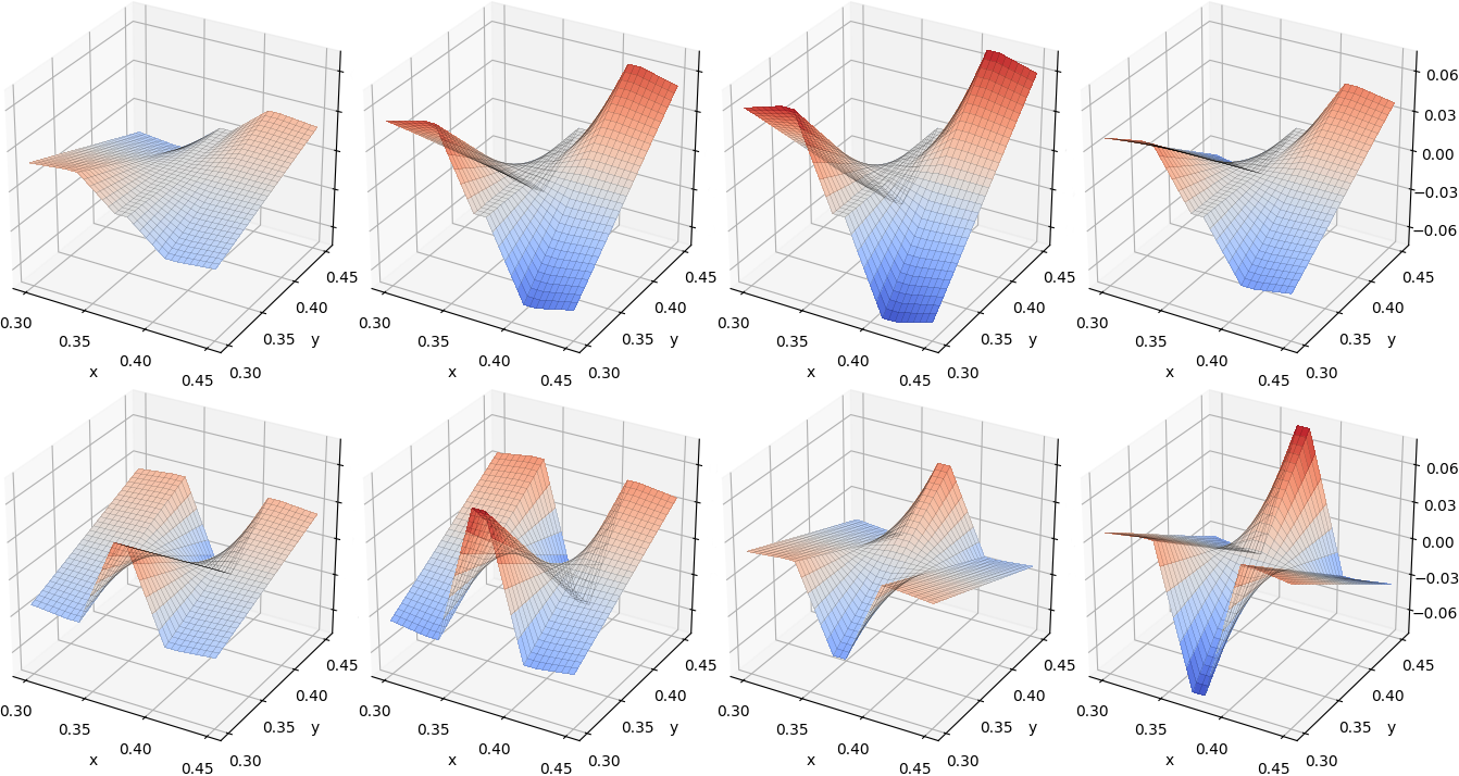
To analyze the transfer eigenvalue problem Eq. 3.3, we first consider a test case including high conductivity channels with high contrast and refer to this numerical example as Example 1. We choose , , and study different sizes of oversampling, ranging from to layers; in detail . We discretize the local domains with a regular quadrilateral mesh with mesh size in both directions and the time interval by equidistant time steps. For numerical accuracy we employ in this subsection an implicit Euler time stepping. Furthermore, we consider zero to three high conductivity channels positioned at , where in the channels and else. Fig. 4 shows that the singular values of the transfer operator first have a plateau and then decay exponentially, where the plateau is longer for a larger number of channels. This is due to the fact that the eigenfunctions corresponding to the singular values located in the plateau contain most energy in the local domain and one can observe variations within the channels as exemplarily shown in Fig. 6. The more channels, the more variations are possible. However, the exponential decay of the singular values is faster if the plateau is longer as already observed for the Helmholtz equation in [15]. Furthermore, we see in Fig. 5 that the singular values decay faster if we increase the number of oversampling layers, where simultaneously the computational costs increase. However, if we compare the eigenfunctions corresponding to different oversampling sizes we can observe that these show very similar dynamics. We therefore conjecture that less oversampling is already sufficient to extract the significant modes.
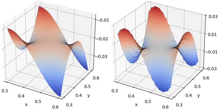
Next, we investigate a model problem including multiscale structure with respect to space and time, which we denote as Example 2. We consider , , and (1 layer of oversampling). Moreover, we use a regular quadrilateral mesh with mesh size in both directions for the spatial discretization and a step size of for the implicit Euler time stepping. We consider and compare the cases (only coarse scale) and (additionally including fine scale). In Fig. 7 we observe that the rapid singular value decay is almost identical for and . Therefore, we can conclude that at least for this test case we do not require a higher number of local reduced basis functions for the approximation of the more complex problem including multiscale behavior regarding space and time. Finally, Fig. 8 exemplarily shows that, as expected, the eigenfunctions inherit the multiscale structure of the problem.
6.2. Global GFEM approximation with random local basis generation
In this subsection we analyze the global GFEM approximation constructed from local reduced spaces that were generated using randomization to enable a more efficient computation; in detail we used Algorithms 2 and 3 in subsection SM2.2 and section SM3.1313 13 Following the notation in subsection SM2.2 and section SM3 we use a local and global failure probability of and test vectors. For an intense study on how the results of the randomized algorithm depend on parameters such as the number of test vectors see [15]. Throughout the whole subsection we consider the time interval and the global spatial domain decomposed into local domains of size with an overlap of size . We also use an oversampling size of . To ensure that the CFL condition for the numerical accuracy of the space-time Petrov-Galerkin discretization is satisfied (cf. [2]), we discretize the computational domain either with a regular quadrilateral mesh with mesh size in both directions and time step size (discretization 1) or with mesh size and time step size (discretization 2).

We analyze two test cases: First, we consider a constant coefficient with right hand side and homogeneous initial and Dirichlet boundary conditions. Hence, the analytical solution is known. We refer to this numerical example as Example 3.1 (discretization 1) and 3.2 (discretization 2) depending on which discretization is used. Secondly, we investigate a model problem including high contrast with respect to space and time in terms of high conductivity channels that are switched on and off over time (Example 4 in the following). To this end, we define a heating region , a cooling region , and a channel region as depicted in Fig. 9. Note that the channels are switched on and off at certain time points. We assume that for , else, for , for , and else. Moreover, we prescribe homogeneous initial and Dirichlet boundary conditions and use discretization 2.
| local basis size | 10 | 25 | 50 | 100 | 200 | 300 | 400 | 500 | 600 | 700 | 800 |
|---|---|---|---|---|---|---|---|---|---|---|---|
| inf-sup constant | 0.99 | 0.99 | 0.99 | 0.99 | 0.99 | 0.99 | 0.99 | 0.98 | 0.95 | 0.91 | 0.87 |
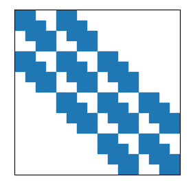
While we cannot guarantee stability of the global approximation in general, we observe in Table 1 that for Example 3.1 the inf-sup constant is close to one and we thus have stability. Fig. 10 shows that the global error1414 14 convergence is clearly guided by the local error1515 15 convergence, which is in turn very similar to the singular value decay. This is in line with the predictions by theory, cf. Section 5.1. Although we only use layers of oversampling for the computation of the local reduced spaces this seems to be sufficient to yield good approximation properties and extract the significant modes which confirms the conjecture in Section 6.1 at least for the given numerical examples. If we have a closer look at the results for Example 3.1, we observe that for increasing local basis sizes the global error behavior seems to change as shown in Fig. 11 (left). However, this can be traced back to the coarse spatial discretization since the result for the finer discretization employed in Example 3.2 again shows that the global errors exactly follow the local errors (cf. Fig. 11 (right)). For the results shown in Figs. 12 and 13 we used the adaptive randomized Algorithms 2 and 3 introduced in subsection SM2.2 and section SM31616 16 Since we assume that for Example 3 and 4 (thus ), we used Algorithm 3 with the improved relative global error bound (cf. Proposition 5.5) to generate the results shown in Fig. 13. and chose equal to one due to the results observed in Table 1. Algorithm 3 enables us to prescribe a global error tolerance and generate an approximation that satisfies the desired tolerance with probability (). In Fig. 13 we observe that in our numerical experiments the algorithm always succeeded and the same holds true for the outcome of Algorithm 2 (cf. Fig. 12). The local1717 17 (global1818 18 ) results are more accurate than required by about to ( to ) orders of magnitude. The former is due to the fact that Algorithm 2 constructs local spaces that have better approximation properties than required, where the latter is additionally caused by the pessimistic global a priori error bound (cf. Proposition 5.5) that is employed to calculate local error tolerances from the prescribed global error tolerance in Algorithm 3. Finally, Fig. 14 shows the sparsity pattern of the global reduced system matrix, where the block sparsity structure results from the overlap of neighboring local subdomains.
7. Conclusions
We have proposed local space-time ansatz spaces for linear parabolic PDEs that are optimal in the sense of Kolmogorov [47] and can be used in domain decomposition and multiscale methods. The diffusion coefficient of the PDE may be arbitrarily rough with respect to both space and time. The optimal local spaces are spanned by the left singular values of a compact transfer operator that acts on the space of local solutions. Moreover, we have employed a space-time GFEM to couple the local ansatz spaces and construct an approximation of the global solution. Furthermore, we have derived rigorous local and global a priori error bounds. In particular, we have shown that the global approximation error in a suitable graph norm can be bounded only by the local approximation errors in the -seminorm. Finally, we have proposed an adaptive algorithm for the localized construction of the local ansatz spaces such that the global GFEM approximation satisfies a desired global error tolerance.
The numerical experiments demonstrate a very rapid and exponential decay of the singular values of the transfer operator and the local and global approximation errors for problems with high contrast or multiscale structure regarding both the spatial and the temporal variable. Since in addition no time stepping procedure is required, the computation of the global approximation is very efficient. For a multiscale test case we have observed that the singular values of the transfer operator seem to be independent of the size of the parameter that determines the periodicity of fine-scale variations in the diffusion coefficient. We conjecture that this result transfers to at least for the considered test case. Moreover, we have observed that the global error convergence is clearly guided by the local error convergence as predicted by theory. Our numerical experiments have shown that the global reduced inf-sup constant is close to one and we thus have stability at least for the considered test cases.
For future applications it is favorable to investigate numerically more efficient discretization techniques such as low rank tensor formats (cf. [34] and references therein).
Appendix A Proofs
A.1. Proofs of Section 3.2
In the remainder of this subsection we denote the inner product by and the dual pairing between and its dual space by . Analogously, we define and .
Proof of Proposition 3.1 (Parabolic Caccioppoli inequality).
Since is contained in , we have that for all and . As is chosen arbitrarily the fundamental lemma of calculus of variations yields that for almost every
| (A.1) |
Let denote a cut-off function with the following properties: , in , and . Additionally choose arbitrarily. In the following we want to use as a test function. However, we cannot apply partial integration in time since the function is contained in , but not in . We therefore approximate by a sequence such that (to simplify the notation we omit the restriction ). Then, we have that for almost every and each and for almost every according to Eq. A.1. Consequently, integrating over time yields for each . Since does not depend on time, we can infer that
This implies that . As in the sequence especially converges weakly in . Hence, we can conclude that
Finally, we apply partial integration in time and exploit in to obtain . By applying the Cauchy-Schwarz and Young’s inequality we have that
By exploiting the properties of the cut-off function we infer that
| (A.2) |
Bounding each term in Eq. A.2 by and taking in both inequalities the supremum over all yields the estimate. ∎
Proof of Lemma 3.2 (Regularity).
Let a function be given. Employing partial integration in time, we have that
Here, the linear operator , , is induced by the linear operator , . Since the space is a dense subspace of , we apply the Hahn-Banach theorem to infer that
It follows that . The result for can be shown analogously. ∎
Theorem A.1 (Compactness of transfer operator).
The transfer operator introduced in Eq. 3.1 is compact.
Proof.
Let denote a sequence that is bounded with respect to . Consequently, the sequence is bounded in . Then, there exists a subsequence that converges weakly to a limit function . Next, we show that . The weak convergence yields since we have for every . Exploiting arguments completely analogous to the proof of Lemma 3.2, we obtain , thus 1919 19 Recall that . and thanks to the embedding we have . It remains to show that satisfies homogeneous initial conditions. For and we infer that
Exploiting the density of in thus yields that converges weakly-* to in . Choosing test functions and satisfying we can conclude
As is arbitrary and is dense in it follows that in . Hence, the limit is an element of .
As is bounded in thanks to Lemma 3.2, the compactness theorem of Aubin-Lions [65, Corollary 5] then yields a subsequence which converges strongly to in due to the uniqueness of weak limits. Considering the error sequence , we thus have that in . Since each is contained in , the parabolic Caccioppoli inequality Eq. 3.2 yields and we obtain in . ∎
Proposition A.2 (Parabolic Poincaré inequality).
There exists a constant such that for all functions
| (A.3) |
An analogous result holds for functions in .
Similar parabolic Poincaré inequalities can, for instance, be found in [4, Theorem 2.2], [44, Lemma 2.5], and [70, Lemma 3]. However, the idea of the proof of inequality Eq. A.3 is guided by the proof of the (elliptic) Poincaré inequality (see [27, Theorem 1, section 5.8]).
Proof.
We provide the proof for the case of a function , the case follows analogously. First, we derive an auxiliary result which demonstrates that a function in that is constant in space for all time points is zero. In a second step the parabolic Poincaré inequality is proved by contradiction.
Let satisfy almost everywhere in for almost every . Since we have , it follows that in . Consequently, is constant in space and time. Thanks to the homogeneous initial values prescribed for functions in , we obtain almost everywhere in for almost every .
Subsequently, the inequality is proved by contradiction as follows: Suppose the assertion of the lemma is false. Then for all we can find a function satisfying . Without loss of generality we can moreover suppose that for all .2020 20 Otherwise we consider the normalized sequence . We therefore have for all . Hence, the sequence is bounded in and there exists a subsequence and a limit such that in . Following completely analogous arguments as employed in the proof of Theorem A.1 we can exploit this weak convergence to infer that . Furthermore, the arguments employed in the proof of Theorem A.1 additionally yield a subsequence which converges strongly to in . Moreover, the subsequence of gradients converges strongly to in by construction. We can thus infer that and in . Since satisfies almost everywhere in for almost every , the auxiliary result verified in the first step of this proof yields almost everywhere in for almost every . However, this is in contradiction to . ∎
A.2. Proofs of Section 3.3
Proposition A.3 (Parabolic Caccioppoli inequality).
For a function and thus the following estimate holds:
Proof.
The proof follows from analogous arguments as employed in the proof of the parabolic Caccioppoli inequality Eq. 3.2 (see Section A.1), considering a cut-off function with the properties , in , on , and in . Moreover, we choose on if and on else. ∎
Proposition A.4 (Parabolic Poincaré inequality).
There exists a constant such that for all functions
An analogous result holds for functions in .
Proof.
The proof is analogous to the proof of the Poincaré inequality Eq. A.3. ∎
Theorem A.5 (Compactness of transfer operator).
The transfer operator introduced in Eq. 3.6 is compact.
Proof.
The proof is analogous to the proof of Theorem A.1. ∎
A.3. Proofs of Section 5.1
Proof of Proposition 5.2 (Local a priori error bound).
First, we define a function in such that we can use Assumption Eq. 5.5, similar to the proof of Proposition SM5.2 in [15]. Subsequently, we bound the remaining terms by the data (cf. the discussion in Remark 5.4). We provide the proof for subdomains located at the boundary of . For subdomains located in the interior the proof is slightly easier. We define the following function :2121 21 To simplify the notation we omit the subscript . For the definition of or see Section 3.3.
| (A.4) |
Here, we assume without loss of generality that and are orthogonal with respect to the inner product. The coefficients will be identified below. Since solves , can be decomposed in the following way
| (A.5) |
where . Consequently, for we have that
where . Therefore, we can conclude
We then choose as the best approximation of in and thus define , where are the eigenfunctions of the transfer eigenvalue problem. Assumption Eq. 5.5 then yields
Thus, we can so far conclude that
Thanks to Eq. A.5, it holds that . Using the density of in 2222 22 Note that ., the Cauchy-Schwarz and Young’s inequality, we obtain
where the constant is given by . Since we have , we can conclude that . ∎
Proof of Proposition 5.5 (Global GFEM error bound).
First, we use a (Petrov-)Galer-kin orthogonality of the global approximation error and the reduced test space to bound the time derivative of the global error in the -norm in terms of the global error in the -seminorm. Subsequently, we introduce a function in that is adapted for exploiting the local a priori error bound Eq. 5.7. To finally make use of the latter, we exploit that functions in solve the PDE locally. Since is dense in , we note that for any 2323 23 Recall that with .
| (A.6) | ||||
Therefore, we obtain . By using the triangle inequality we have that for any
Assumption Eq. 5.3 regarding inf-sup-stability and Eq. A.6 yield
| (A.7) |
In the following we choose with local approximations as introduced in the proof of Proposition 5.2 (see Eq. A.4). To be able to exploit the local a priori error bound Eq. 5.7, we bound the first term in Eq. A.7 by the sum of local -seminorms of . To employ that solves the PDE locally, we approximate by a sequence with , , and , such that in . It follows that
Since (cf. Eq. A.4 in the proof of Proposition 5.2) and does not depend on time, we obtain
Furthermore, the properties of the partition of unity Eq. 5.1 yield
Consequently, we may infer that
As an intermediate result we therefore obtain
Exploiting the definition of , Young’s inequality, the Cauchy-Schwarz inequality, the overlap condition, and the properties of the partition of unity, it follows that
Since , we infer analogously to the proof of the parabolic Poincaré inequality (Propositions A.2 and A.4) that there exists a constant such that
We can finally employ Assumption Eq. 5.7 and obtain
where the constant is defined as and is given by if and else. Exploiting the overlap condition Eq. 5.2 it follows that
Finally, we have
where the constant is given by . ∎
Acknowledgments
The authors would like to thank the anonymous referees for their constructive comments, which helped to improve the presentation of the paper.
References
- [1] F. Albrecht, B. Haasdonk, S. Kaulmann, and M. Ohlberger, The localized reduced basis multiscale method, in Proceedings of Algoritmy 2012, Conference on Scientific Computing, Vysoke Tatry, Podbanske, 2012, Slovak University of Technology in Bratislava, Publishing House of STU, 2012, pp. 393–403.
- [2] R. Andreev, Stability of space-time Petrov-Galerkin discretizations for parabolic evolution equations, PhD thesis, ETH Zürich, Zürich, 2012.
- [3] R. Andreev, Stability of sparse space-time finite element discretizations of linear parabolic evolution equations, IMA J. Numer. Anal., 33 (2013), pp. 242–260.
- [4] J. Aramaki, Poincare inequality and Campanato estimates for weak solutions of parabolic equations, Electron. J. Differential Equations, (2016), pp. 1–8.
- [5] I. Babuška and J. Osborn, Can a finite element method perform arbitrarily badly?, Math. Comp., 69 (2000), pp. 443–462.
- [6] I. Babuška, G. Caloz, and J. E. Osborn, Special finite element methods for a class of second order elliptic problems with rough coefficients, SIAM J. Numer. Anal., 31 (1994), pp. 945–981.
- [7] I. Babuška, X. Huang, and R. Lipton, Machine computation using the exponentially convergent multiscale spectral generalized finite element method, ESAIM Math. Model. Numer. Anal., 48 (2014), pp. 493–515.
- [8] I. Babuška and R. Lipton, Optimal local approximation spaces for generalized finite element methods with application to multiscale problems, Multiscale Model. Simul., 9 (2011), pp. 373–406.
- [9] I. Babuška, R. Lipton, P. Sinz, and M. Stuebner, Multiscale-spectral GFEM and optimal oversampling, Comput. Methods Appl. Mech. Eng., 364 (2020), pp. 112960, 28.
- [10] I. Babuška and J. M. Melenk, The partition of unity finite element method: basic theory and applications, Comput. Methods Appl. Mech. Engrg., 139 (1996), pp. 289–314.
- [11] P. Baroni, A. Di Castro, and G. Palatucci, Global estimates for nonlinear parabolic equations, J. Evol. Equ., 13 (2013), pp. 163–195.
- [12] J. Brunken, K. Smetana, and K. Urban, (Parametrized) first order transport equations: realization of optimally stable Petrov-Galerkin methods, SIAM J. Sci. Comput., 41 (2019), pp. A592–A621.
- [13] A. Buhr, Towards Automatic and Reliable Localized Model Order Reduction, PhD thesis, University of Münster, Münster, 2019.
- [14] A. Buhr, L. Iapichino, M. Ohlberger, S. Rave, F. Schindler, and K. Smetana, Localized model reduction for parameterized problems; in P. Benner, S. Grivet-Talocia, A. Quarteroni, G. Rozza, W.H.A. Schilders, L.M. Sileira (eds.). Model Order Reduction, Volume 2, Snapshot-Based Methods and Algorithms, Walter De Gruyter GmbH, Berlin, 2021.
- [15] A. Buhr and K. Smetana, Randomized local model order reduction, SIAM J. Sci. Comput., 40 (2018), pp. A2120–A2151.
- [16] K. Chen, Q. Li, J. Lu, and S. J. Wright, Randomized Sampling for Basis Function Construction in Generalized Finite Element Methods, Multiscale Model. Simul., 18 (2020), pp. 1153–1177.
- [17] Y. Chen, T. Y. Hou, and Y. Wang, Exponential Convergence for Multiscale Linear Elliptic PDEs via Adaptive Edge Basis Functions, 2020, https://arxiv.org/abs/2007.07418.
- [18] M. Choulli, Local boundedness property for parabolic BVP’s and the Gaussian upper bound for their Green functions, Evol. Equ. Control Theory, 4 (2015), pp. 61–67.
- [19] E. T. Chung, Y. Efendiev, W. T. Leung, and S. Ye, Generalized multiscale finite element methods for space-time heterogeneous parabolic equations, Comput. Math. Appl., 76 (2018), pp. 419–437.
- [20] W. Dahmen, C. Huang, C. Schwab, and G. Welper, Adaptive Petrov-Galerkin methods for first order transport equations, SIAM J. Numer. Anal., 50 (2012), pp. 2420–2445.
- [21] L. Demkowicz and J. Gopalakrishnan, A class of discontinuous Petrov-Galerkin methods. Part I: the transport equation, Comput. Methods Appl. Mech. Engrg., 199 (2010), pp. 1558–1572.
- [22] L. Demkowicz and J. Gopalakrishnan, A class of discontinuous Petrov-Galerkin methods. II. Optimal test functions, Numer. Methods Partial Differential Equations, 27 (2011), pp. 70–105.
- [23] L. Diening and J. Storn, A Space-Time DPG Method for the Heat Equation, tech. report, arXiv:2012.13229, 2020, https://arxiv.org/pdf/2012.13229.pdf.
- [24] W. E and B. Engquist, The heterogeneous multiscale methods, Commun. Math. Sci., 1 (2003), pp. 87–132.
- [25] Y. Efendiev, J. Galvis, and T. Y. Hou, Generalized multiscale finite element methods (GMsFEM), J. Comput. Phys., 251 (2013), pp. 116–135.
- [26] J. L. Eftang and A. T. Patera, Port reduction in parametrized component static condensation: approximation and a posteriori error estimation, Int. J. Numer. Methods Eng., 96 (2013), pp. 269–302.
- [27] L. C. Evans, Partial differential equations, vol. 19 of Grad. Stud. Math., American Mathematical Society, Providence, RI, second ed., 2010.
- [28] G. R. Feijóo, T. J. R. Hughes, L. Mazzei, and J.-B. Quincy, The variational multiscale method—a paradigm for computational mechanics, Comput. Methods Appl. Mech. Engrg., 166 (1998), pp. 3–24.
- [29] A. Ferrero, A. Iollo, and F. Larocca, Global and local POD models for the prediction of compressible flows with DG methods, Int. J. Numer. Methods Eng., 116 (2018), pp. 332–357.
- [30] M. J. Gander, Optimized Schwarz methods, SIAM J. Numer. Anal., 44 (2006), pp. 699–731.
- [31] M. Ghasemi and E. Gildin, Localized model order reduction in porous media flow simulation, J. Pet. Sci. Eng., 145 (2016), pp. 689–703.
- [32] G. H. Golub and C. F. Van Loan, Matrix computations, Johns Hopkins Studies in the Mathematical Sciences, Johns Hopkins University Press, Baltimore, MD, fourth ed., 2013.
- [33] L. Grasedyck, I. Greff, and S. Sauter, The AL basis for the solution of elliptic problems in heterogeneous media, Multiscale Model. Simul., 10 (2012), pp. 245–258.
- [34] L. Grasedyck, D. Kressner, and C. Tobler, A literature survey of low-rank tensor approximation techniques, GAMM-Mitteilungen, 36 (2013), pp. 53–78.
- [35] M. Griebel and M. A. Schweitzer, A particle-partition of unity method for the solution of elliptic, parabolic, and hyperbolic PDEs, SIAM J. Sci. Comput., 22 (2000), pp. 853–890.
- [36] N. Halko, P. G. Martinsson, and J. A. Tropp, Finding structure with randomness: probabilistic algorithms for constructing approximate matrix decompositions, SIAM Rev., 53 (2011), pp. 217–288.
- [37] A. Heinlein, A. Klawonn, J. Knepper, and O. Rheinbach, Multiscale coarse spaces for overlapping Schwarz methods based on the ACMS space in 2D, Electron. Trans. Numer. Anal., 48 (2018), pp. 156–182.
- [38] T. Y. Hou and X.-H. Wu, A multiscale finite element method for elliptic problems in composite materials and porous media, J. Comput. Phys., 134 (1997), pp. 169–189.
- [39] T. J. R. Hughes and J. R. Stewart, A space-time formulation for multiscale phenomena, vol. 74, 1996, pp. 217–229. TICAM Symposium (Austin, TX, 1995).
- [40] D. B. P. Huynh, D. J. Knezevic, and A. T. Patera, A static condensation reduced basis element method: Approximation and a posteriori error estimation, ESAIM. Math. Model. Numer. Anal., 47 (2013), pp. 213–251.
- [41] L. Iapichino, A. Quarteroni, and G. Rozza, A reduced basis hybrid method for the coupling of parametrized domains represented by fluidic networks, Comput. Methods Appl. Mech. Eng., 221/222 (2012), pp. 63–82.
- [42] M. Kapteyn, D. Knezevic, D. Huynh, M. Tran, and K. Willcox, Data-driven physics-based digital twins via a library of component-based reduced-order models, Int. J. Numer. Methods Eng., (2020).
- [43] S. Kaulmann, B. Flemisch, B. Haasdonk, K.-A. Lie, and M. Ohlberger, The localized reduced basis multiscale method for two-phase flows in porous media, Int. J. Numer. Methods Eng., 102 (2015), pp. 1018–1040.
- [44] S. Kim, Gaussian estimates for fundamental solutions of second order parabolic systems with time-independent coefficients, Trans. Amer. Math. Soc., 360 (2008), pp. 6031–6043.
- [45] A. Klawonn, O. B. Widlund, and M. Dryja, Dual-primal FETI methods for three-dimensional elliptic problems with heterogeneous coefficients, SIAM J. Numer. Anal., 40 (2002), pp. 159–179.
- [46] D. J. Knezevic, H. Kang, P. Sharma, G. Malinowski, T. T. Nguyen, et al., Structural Integrity Management of Offshore Structures via RB-FEA and Fast Full Load Mapping Based Digital Twins, in The 28th International Ocean and Polar Engineering Conference, International Society of Offshore and Polar Engineers, 2018.
- [47] A. Kolmogoroff, Über die beste Annäherung von Funktionen einer gegebenen Funktionenklasse, Ann. of Math. (2), 37 (1936), pp. 107–110.
- [48] R. B. Lehoucq, D. C. Sorensen, and C. Yang, ARPACK users’ guide: solution of large-scale eigenvalue problems with implicitly restarted Arnoldi methods, SIAM, 1998.
- [49] J.-L. Lions and E. Magenes, Non-homogeneous boundary value problems and applications. Vol. II, Springer-Verlag, New York-Heidelberg, 1972.
- [50] Y. Maday and E. M. Rønquist, A reduced-basis element method, J. Sci. Comput., 17 (2002), pp. 447–459.
- [51] Y. Maday and E. M. Rønquist, The Reduced Basis Element Method: Application to a Thermal Fin Problem, SIAM J. Sci. Comput., 26 (2004), pp. 240–258.
- [52] A. Mlqvist and A. Persson, Multiscale techniques for parabolic equations, Numer. Math., 138 (2018), pp. 191–217.
- [53] A. Mlqvist and D. Peterseim, Localization of elliptic multiscale problems, Math. Comp., 83 (2014), pp. 2583–2603.
- [54] I. Martini, G. Rozza, and B. Haasdonk, Reduced basis approximation and a-posteriori error estimation for the coupled Stokes-Darcy system, Adv. Comput. Math., 41 (2015), pp. 1131–1157.
- [55] P. Ming and P. Zhang, Analysis of the heterogeneous multiscale method for parabolic homogenization problems, Math. Comp., 76 (2007), pp. 153–177.
- [56] K. Nyström, H. Persson, and O. Sande, Boundary estimates for solutions to linear degenerate parabolic equations, J. Differential Equations, 259 (2015), pp. 3577–3614.
- [57] H. Owhadi, Multigrid with rough coefficients and multiresolution operator decomposition from hierarchical information games, SIAM Rev., 59 (2017), pp. 99–149.
- [58] H. Owhadi and L. Zhang, Localized bases for finite-dimensional homogenization approximations with nonseparated scales and high contrast, Multiscale Model. Simul., 9 (2011), pp. 1373–1398.
- [59] H. Owhadi and L. Zhang, Gamblets for opening the complexity-bottleneck of implicit schemes for hyperbolic and parabolic ODEs/PDEs with rough coefficients, J. Comput. Phys., 347 (2017), pp. 99–128.
- [60] H. Owhadi, L. Zhang, and L. Berlyand, Polyharmonic homogenization, rough polyharmonic splines and sparse super-localization, ESAIM Math. Model. Numer. Anal., 48 (2014), pp. 517–552.
- [61] A. Pinkus, n-widths in approximation theory, vol. 7 of Ergeb. Math. Grenzgeb. (3), Springer-Verlag, Berlin, 1985.
- [62] M. Renardy and R. C. Rogers, An introduction to partial differential equations, vol. 13, Springer Science & Business Media, 2004.
- [63] J. Schleuß, Source code to “Optimal local approximation spaces for parabolic problems”, 2020, https://doi.org/10.5281/zenodo.4275561.
- [64] C. Schwab and R. Stevenson, Space-time adaptive wavelet methods for parabolic evolution problems, Math. Comput., 78 (2009), pp. 1293–1318.
- [65] J. Simon, Compact sets in the space , Ann. Mat. Pura Appl. (4), 146 (1987), pp. 65–96.
- [66] K. Smetana, Static condensation optimal port/interface reduction and error estimation for structural health monitoring, in IUTAM Symposium on Model Order Reduction of Coupled Systems, Stuttgart, Germany, May 22–25, 2018, Springer, 2020, pp. 1–24.
- [67] K. Smetana and A. T. Patera, Optimal local approximation spaces for component-based static condensation procedures, SIAM J. Sci. Comput., 38 (2016), pp. A3318–A3356.
- [68] N. Spillane, V. Dolean, P. Hauret, F. Nataf, C. Pechstein, and R. Scheichl, Abstract robust coarse spaces for systems of PDEs via generalized eigenproblems in the overlaps, Numerische Mathematik, 126 (2014), pp. 741–770.
- [69] R. Stevenson and J. Westerdiep, Stability of Galerkin discretizations of a mixed space-time variational formulation of parabolic evolution equations, IMA J. Numer. Anal., 41 (2021), pp. 28–47.
- [70] M. Struwe, On the Hölder continuity of bounded weak solutions of quasilinear parabolic systems, Manuscripta Math., 35 (1981), pp. 125–145.
- [71] T. Taddei and A. T. Patera, A localization strategy for data assimilation; application to state estimation and parameter estimation, SIAM J. Sci. Comput., 40 (2018), pp. B611–B636.
- [72] K. Urban and A. T. Patera, An improved error bound for reduced basis approximation of linear parabolic problems, Math. Comput., 83 (2014), pp. 1599–1615.