Challenging common interpretability assumptions in feature attribution explanations

Jonathan Dinu Affiliation: Unaffiliated Email: jdinu@berkeley.edu Jeffrey Bigham Affiliation: Human-Computer Interaction Institute Affiliation: Carnegie Mellon University Email: jbigham@cs.cmu.edu J. Zico Kolter Affiliation: School of Computer Science Affiliation: Carnegie Mellon University Email: zkolter@cs.cmu.edu

Abstract

As machine learning and algorithmic decision making systems are increasingly being leveraged in high-stakes human-in-the-loop settings, there is a pressing need to understand the rationale of their predictions. Researchers have responded to this need with explainable AI (XAI), but often proclaim interpretability axiomatically without evaluation. When these systems are evaluated, they are often tested through offline simulations with proxy metrics of interpretability (such as model complexity). We empirically evaluate the veracity of three common interpretability assumptions through a large scale human-subjects experiment with a simple “placebo explanation” control. We find that feature attribution explanations provide marginal utility in our task for a human decision maker and in certain cases result in worse decisions due to cognitive and contextual confounders. This result challenges the assumed universal benefit of applying these methods and we hope this work will underscore the importance of human evaluation in XAI research. Supplemental materials—including anonymized data from the experiment, code to replicate the study, an interactive demo of the experiment, and the models used in the analysis—can be found at: https://doi.pizza/challenging-xai.

1 Introduction

With algorithmic and autonomous systems becoming more ubiquitous in everyday life, there has been a new interest [34] in understanding users’ perceptions [48] of these systems, as well as the behavior [63] of these systems in the human context in which they are deployed [3, 13]. This is due to emerging societal concerns [18] and the legal demands of regulatory frameworks such as the EU General Data Protection Regulation’s “right to explanation” [64], in addition to the more ambiguous collective apprehension of the public [9, 48, 70]. While much of the field of machine learning (and much of the public) has rallied around the call for interpretable [33, 55], transparent [36], and fair algorithms [7] as a solution to mitigate the potential unintended consequences of real world applications of these systems, little behavioral inquiry [58] has been conducted into what actually makes an algorithm understandable or if interpretability is even desirable and beneficial [49].

Although common in fields like economics, political science, and psychology [59] (as well as industry practice [4, 21, 38]), traditional computer science and machine learning research has typically not needed to leverage empirical methods or conduct experiments with human subjects. When these systems have been evaluated systematically with human subjects, the gold standard for quantifying the utility of an explanation is some self defined measure of interpretability. This approach however is fraught with epistemological difficulties since researchers often use different notions of interpretability, making any systematic comparisons between new XAI systems difficult (if not impossible) unless a wholly new human subjects experiment is run [22]. If a researcher attempts to replicate a previous evaluation, even if the experiment is well documented and published, subtle confounders—as seemingly innocuous (for machine learning evaluation) as the colors used in the interface [66, 68]—can result in conclusions that overstate the strength of evidence [42]. The epistemological difficulties of measuring interpretability compound with the potential for uncontrolled experimental confounders, resulting in unreplicable research at best—and pernicious evaluations of XAI systems at worst.

2 Axiomatic assumptions

While it is unrealistic to systematically evaluate and validate every-single-possible-design-decision with a rigorous human subjects experiment, often the pendulum swings too far in the opposite direction, with researchers making conveniently favorable interpretability claims about their systems. For a proper exposition of the more frequent assumptions (and the damage they can do) we refer readers to Lipton. For the purposes of this paper and our experiment, we focused on the follow three assumptions as they apply to post-hoc feature attribution explanations [52].

Simpler models are more interpretable.

There seems to be a prevailing opinion in the ML community [67, 69] that simple models (like linear regressions or decision trees) are tautologically¹¹ 1 By its nature of being simple, it is interpretable. And since it is interpretable, it is necessarily simple (to understand). more interpretable than complex models (like neural networks). Besides the cheeky fact of the equivalence between a (very simple) one layer neural network and least squares linear regression, model complexity can often be a misleading proxy of interpretability [22].

Model-agnostic methods are data, task, and user agnostic.

By extension of the first assumption, model-agnostic post-hoc explanation methods [65, 52] implicitly assume that simple explanations are more interpretable than complex explanations. And as such, a complex model can be made interpretable with a simple explanation as long as the explainer is verisimilar [61] to the original model. Other externalities (in the non-economic sense) however can have an outsized effect on a human’s ability to interpret a model [41, 45].

Any explanation is better than no explanation.

One might intuit that a post-hoc explanation would never lead to a worse decision than one made using the same underlying model absent explanation. Recent research however has shown that not only are XAI methods innocuously fragile in practice [43, 47], they are also susceptible to adversarial intervention [1, 71, 46]. In additional to these algorithmic issues, irreducible cognitive factors and intrinsic human biases [32, 23, 31] can perpetuate harmful effects in any algorithmically aided decision making context (explanations or not).

3 Replication as retrospective

While researchers have identified the need for more consistent measures of fairness [54, 17, 37], much of the prior empirical XAI research uses different definitions of interpretability, quantified through disparate proxies [8, 44, 16, 57, 30, 25, 2, 5]. This diversity of measures compounds with the already well known methodological issues of null hypothesis statistical testing [29, 40, 19] to create research pathologies [35, 28] that can precipitate potentially misleading conclusions.

Experiment design.

To efficiently interrogate the above assumptions—while at the same time evaluating the external validity of previous research findings [65, 62]—we ran a mixed between/within-subjects repeated measures experiment [56] on Amazon’s Mechanical Turk [53] with 796 participants. To address the previously stated challenges of rigorously evaluating XAI systems with human subjects—and to build a methodology that can be used by other researchers in the field—we posit that interpretability is not directly measurable. Instead, we use a model grounded in psychometric theory [74] to infer the subject’s latent ability to interpret from a series of measurable pairwise comparisons.

To emulate an authentic task and minimize any confounding from differences in domain knowledge, the experiment presented regression models that predicted the price of Airbnb listings. The underlying black box models were trained with real Airbnb listing data sourced from Inside Airbnb, which includes various features of the listings (# of bedrooms, number of reviews, review scores, etc.).²² 2 Appendix 3 contains a description of the features used in our experiment. A single experimental run consisted of ten trials (pairwise comparisons). In each trial, the subject was presented with explanations of two underlying models and asked to determine which model would perform more accurately in the real world (Figure 1).

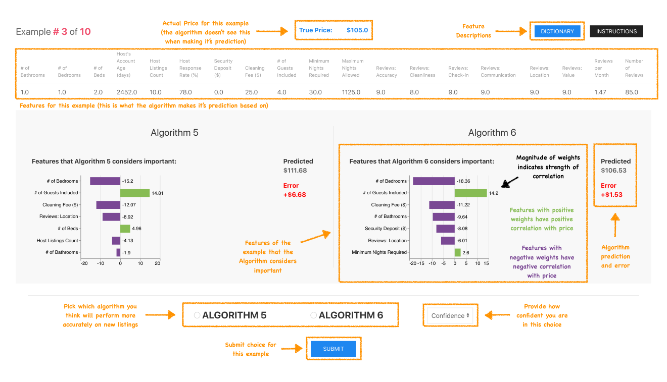
Refer to caption — Figure 1: An annotated interface for a single trial. The subject was presented with this annotated interface in the instructions, but each trial was presented with the annotations (in orange) removed. The precise instructions presented to each subject at the beginning of the experiment along with the other minutia of conducting the experiment can be found in Appendix A. For this example, the data is dense and the top 7 features are shown (the explainer cannot be discerned through the interface alone). Additionally, a demo of the experiment can anonymously be completed at http://xai.jonathan.industries.

To establish a ground truth for this task, we followed a construction similar to Ribeiro et al.. The comparisons in the experiment explained two different underlying black box models³³ 3 For the ridge and lasso variants of the explainer factor, the explanation and the model are the same. which were intentionally setup to exhibit a test set accuracy discrepancy (Appendix 5). To consistently introduce a discrepancy that could plausibly be encountered in a real task, we leveraged the multi-city dataset of Inside Airbnb to simulate dataset shift.

The underlying black box models for each explainer were trained and validated with either listings from New York City (NYC) or Los Angeles (LA).⁴⁴ 4 A convenience of the Inside Airbnb data is that the features are consistent across cities. During training, the amount of regularization was manipulated to match accuracy for all models within a city (i.e. the ridge and lasso models for LA had comparable validation accuracy) but to exhibit a validation discrepancy between cities (i.e. LA models had a higher validation accuracy than NYC models). For the test set accuracy however, both models were evaluated against the same test set of NYC listings, which led to a discrepancy in performance (with the LA model predictably performing worse). We consider a response correct if the subject selected the explanation that corresponded to the underlying model with the higher test set accuracy (i.e. the explanation for the NYC model).

To avoid the ambiguity of any notion of interpretability and to state the objective of our experiment precisely: we evaluated the augmentative capabilities of model explanation methods in helping a human decision maker identify a more accurate machine learning model.

Factors.

Our experiment had between-subjects factors of the explanation method used (explainer) and the sparsity of the data. We compared one post-hoc feature attribution method [52] to two “simple” models—ridge ( $l_{2}$ ) and lasso ( $l_{1}$ ) regression—commonly believed to be inherently interpretable [67], even though such interpretations of the model parameters can falsely attribute importance [72] (unless appropriate measures are taken [6, 14]). To serve as a control, we used a fourth condition made up of random feature importances,⁵⁵ 5 For each of top- $n$ random features, we sample importance weights from a symmetric Dirichlet distribution. meant to represent a “placebo explanation”.

For the data sparsity factor, the underlying data examples used for the black box model training (as well as for the explanations) were the same across the two variants. The only difference between the dense variant and sparse variants were the features used. The dense variant contained 19 numeric features (all of which had values), whereas the sparse variant included eight additional features (two continuous and six one-hot encoded categorical). A description of the features used in the experiment, as well as the difference between the dense and sparse variants can be seen in Appendix 3.

Within-subjects factors of top- $n$ features (as calculated from the explainer importance scores) and the data instance (item) explained are varied across the ten trials. A summary of the experimental factors and their levels can be seen in Table 1 and the treatment randomization process is presented in Appendix 1.

To control for possible confounders due to the visualization of explanations, we presented all explainers’ feature attributions as identically styled horizontal bar charts (Figure 1). Subjects are nested within the cross of the between-subjects factors such that each subject only encounters a single explainer-sparsity combination throughout the experiment.⁶⁶ 6 We can think about the cross of these two factors as a single explainer-sparsity factor with eight levels. To control for the variability in subjects’ prior knowledge, experience, and any subjective interpretation of the task, each experimental run was composed of ten trials (comparisons) presented in a randomized order—to additionally account for any learning or ordering effects.

Table 1: Experimental factors and levels.

Factor	Type	Cardinality	Levels
Data sparsity	Between-subjects	2	dense, sparse
Explainer	Between-subjects	4	random, ridge, lasso, SHAP
Top $n$ features	Within-subjects	10	$1,3,5,7,9,11,13,15,17,19$
Item	Within-subjects	10	$1,2,3,4,5,6,7,8,9,10$

Reproducibility $\not\equiv$ replicability.

While we did not reproduce the experiments from Ribeiro et al. and Poursabzi-Sangdeh et al. exactly, one would hope that we would arrive at similar conclusions from the results of our experiment (if the prior research’s effects were generalizable and replicable). This really is the essence of the distinction between replications and reproductions [12, 60]. In this spirit, we invite and encourage anyone with the will, time, and resources to replicate the experiment presented here.⁷⁷ 7 The code to run the experiment, as well as our data to contrast results, can be accessed at https://doi.pizza/challenging-xai.

4 Disentangling Interpretability⁸⁸ 8 We use “disentagle” in the colloquial sense rather than in the representation learning sense [50].

Table 2: Percent of correct responses for each variant. Right most column is the aggregate percent correct across both dense and sparse variants. Bottom row is the aggregate percent correct across explainer variants.

	dense	sparse
random	49.5	60.2	54.8
ridge	55.1	46.7	50.9
lasso	54.1	54.3	54.2
SHAP	52.6	69.5	61.6
	52.7	58.2

Uncertainty in human subjects experiments.

We see a peculiar regularity in the raw results of the experiment (Table 2), with the random explanation variant having a 54.8% correct response rate when aggregating across all levels. This is concerning in and of itself, we would expect a number much closer to 50% since there is absolutely no information in these explanations. Even more concerning, when we group by the sparsity of the data, we find that the random explainer on the dense data resulted in 49.5% correct responses, but on the sparse data the percent correct jumps to 60.2%. Across all of our assignments, the order of the black box models is randomized (so we would not expect any "always choose the left model" effects).

A plausible explanation could be that in the absence of any information in the explanation, the participant simply chooses the model with the lower displayed error⁹⁹ 9 Even though the instructions are explicit about not simply choosing the explanation with the lower error. (which results in the correct response in 5/10 examples for the dense variant and 6/10 examples in the sparse variant). These are a lot of assumptions and speculations however, so a proper experiment is necessary to confirm (or disconfirm) this mechanic.

A psychometric model of interpretability.

To estimate the effect of the various experimental factors (and disambiguate potentially confounding effects present in the raw percent correct of responses), we fit a Bayesian multilevel logistic regression model [27] to the subjects’ responses. Since the experiment measured subjects’ performance on a cognitive task, this model alternatively could be viewed as a one-parameter item response model (1PL) with additional item and person covariates [24]. A distinguishing characteristic of item response theory (IRT) is its heterogeneous treatment of both persons and items: persons each have a latent ability parameter ( $\alpha_{\text{person[i]}}$ ) and items each have a latent easiness¹⁰¹⁰ 10 Or difficulty parameter, depending on the sign of the term in the logit ( $\alpha_{\text{person[i]}}\boldsymbol{-}\beta_{\text{item[i]}}$ ). parameter ( $\beta_{\text{item[i]}}$ ).

\displaystyle Pr(y_{i}=1)

\displaystyle=\text{logit}^{-1}(\alpha_{\text{person[i]}}+\beta_{\text{item[i]}}+X_{i}\theta)

In addition to the person and item parameters, our model also includes various covariates derived from the experimental factors and interaction terms, as well as demographic data collected in an exit survey (Appendix 6):

	$\displaystyle X_{i}=$	$\displaystyle\ \text{confidence}+{\color[rgb]{0,1,0}\text{features}}+{\color[rgb]{0,1,0}\text{trial}}+{\color[rgb]{0,1,0}\text{sparsity}}+{\color[rgb]{0,1,0}\text{explainer}}\ +$
		$\displaystyle\ {\color[rgb]{0,0.4453,0.6992}\text{explainer:confidence}}+{\color[rgb]{0,0.4453,0.6992}\text{explainer:features}}+{\color[rgb]{0,0.4453,0.6992}\text{explainer:sparsity}}+{\color[rgb]{0,0.4453,0.6992}\text{features:sparsity}}\ +$
		$\displaystyle\ {\color[rgb]{1,0.1602,0.457}\text{education}}+{\color[rgb]{1,0.1602,0.457}\text{knowledge}_{computer}}+{\color[rgb]{1,0.1602,0.457}\text{knowledge}_{data}}+{\color[rgb]{1,0.1602,0.457}\text{experience}_{computer}}+{\color[rgb]{1,0.1602,0.457}\text{experience}_{data}}$

We fit our models in R [73] using Stan [15] and the brms package [11]. All MCMC chains converged as judged by visual diagnostics [26] as well as by the $\widehat{R}$ convergence diagnostic [10]. The 1PL model with largest number of considered covariates performed best, as evaluated with LOO cross validation [75] and posterior predictive checks [26].

Explainer heterogeneity.

To investigate the assumption that simpler models are more interpretable, we can look to the estimated parameters for the explainer factor (and its interactions). We show a subset of the model parameters that are relevant to this assumption in Figure 2 (a). Everything else being equal, we found that the simplest explainer in our experiment (ridge regression) performed best—which corroborates Poursabzi-Sangdeh et al.. But often the context in which these models are deployed is not as homogenous as a well defined laboratory experiment.

If instead, we consider the interaction between the explainer and the sparsity of the dataset, the effectiveness of the explainers inverts. On a sparse dataset, the ridge explainer performed the worst and SHAP performed the best. To more directly contrast with the finding of Poursabzi-Sangdeh et al. that subjects were able to better simulate the predictions of a model with fewer features, we find no evidence that the number of features has an effect ( $\mathbb{E}$ =0.02, 95% CI=[-0.03,0.06]) on a person’s ability to discern a more accurate model.

While we did not recreate the experiment from Poursabzi-Sangdeh et al. precisely, our study should be an appropriate test of the generalizability of their findings due to the similarity of our study population (novices on Mechanical Turk) and the domain of our task (estimating the price of housing). Our results do not challenge the internal validity of the experiments in Poursabzi-Sangdeh et al., but rather probe the external validity of whether model simulatability is an appropriate proxy for interpretability (however you want to define the term).

Individual differences.

Most prior empirical interpretability research [8, 44, 16, 57, 30, 25, 2, 5] implicitly assumes that every end user is the same and that the data instances being explained have minimal effect on the interpretability of a model. By directly modeling latent person and item parameters (Figure 2 (b,c)), we can begin to challenge these assumptions. Since all intra-person variation is subsumed by the single ability parameter ( $\alpha_{\text{person[i]}}$ ) however, we cannot make any inferences as to the source of this variation.¹¹¹¹ 11 For our given experiment, these latent ability parameters are likely correlated with a person’s prior knowledge, experience with data mining, and perhaps other intrinsic personality traits.

Similar to the ability parameter for persons, all item variation is subsumed into the single easiness parameter for items ( $\beta_{\text{item[i]}}$ ). But unlike $\alpha_{\text{person[i]}}$ , item difficulties are much more discriminative (Figure 2 (b)). The variance in both group-level parameters ( $sd(person)$ , $sd(item)$ ) provides strong evidence to support this user and data heterogeneity to the point of the variation being dominated by the item parameter. For example, even if we (very conservatively) assume the lower 95% CI (0.59) as the true standard deviation of the item parameters, this is larger than every other parameter mean (with the exception of sparse and sparse:ridge)¹²¹² 12 Caution is needed when interpreting this standard deviation however. Since the distribution of $\beta_{\text{item[i]}}$ is very not normal, one cannot use the convenient 68–95–99.7 rule..

Figure 2: Posterior uncertainty intervals. (a) Subset of model parameters. Thick segments represent 50% credible intervals and thinner outer lines represent 95% credible intervals. (b) Item easiness parameters (

\beta_{\text{item[i]}}

), only 95% interval is shown. (c) Person ability parameters (

\alpha_{\text{person[i]}}

) in sorted order, only 95% interval is shown.

5 Limitations

Similar to all the interpretability experiments that came before, our findings have questionable external validity,¹³¹³ 13 All we really measured was whether a novice can infer which of two models has a better test set accuracy when shown ranked feature importances. since any universal measure of interpretability is ill-defined. Additionally, the heterogeneity of data and persons—combined with the large design space of potential methods, tasks, hyperparameters, etc.—makes any exhaustive evaluation intractable [22].

6 Conclusion

As a community, we have lost the forest for the trees in our quest for more complex (and novel) explanation methods. Perhaps to justify more funding (reminiscence of deep learning’s quixotic quest for MNIST accuracy), we have been chasing benchmarks of proxy measures. Hopefully by evaluating more systems and approaching technical research with a critical lens [39], we all can build more usable and humane technology.

Acknowledgments and Disclosure of Funding

We would like to acknowledge the invisible and often thankless labor of the open source maintainers and contributors, without whose work none of this research would be possible. Additionally, we would like to thank Marco Tulio Ribeiro for graciously sharing, explaining, and discussing the specifics of how he ran the experiments for Ribeiro et al., and the reviewers of this paper—whose constructive feedback made the paper much better than it would have been otherwise.

References

[1] U. Aivodji, H. Arai, O. Fortineau, S. Gambs, S. Hara, and A. Tapp. Fairwashing: the risk of rationalization. In K. Chaudhuri and R. Salakhutdinov, editors, Proceedings of the 36th International Conference on Machine Learning, volume 97 of Proceedings of Machine Learning Research, pages 161–170. PMLR. URL http://proceedings.mlr.press/v97/aivodji19a.html.
Al-Shedivat et al. [2020] M. Al-Shedivat, A. Dubey, and E. P. Xing. Contextual explanation networks, 2020.
[3] S. Amershi, D. Weld, M. Vorvoreanu, A. Fourney, B. Nushi, P. Collisson, J. Suh, S. Iqbal, P. N. Bennett, K. Inkpen, and others. Guidelines for human-AI interaction. In Proceedings of the 2019 CHI Conference on Human Factors in Computing Systems, page 3. ACM.
[4] E. Bakshy, D. Eckles, and M. S. Bernstein. Designing and deploying online field experiments. URL https://arxiv.org/abs/1409.3174v1.
Bang et al. [2019] S. Bang, P. Xie, H. Lee, W. Wu, and E. Xing. Explaining a black-box using deep variational information bottleneck approach, 2019.
Barber et al. [2015] R. F. Barber, E. J. Candès, et al. Controlling the false discovery rate via knockoffs. The Annals of Statistics, 43(5):2055–2085, 2015.
[7] S. Barocas, M. Hardt, and A. Narayanan. Fairness and Machine Learning. fairmlbook.org.
Bhatt et al. [2020] U. Bhatt, A. Weller, and J. M. F. Moura. Evaluating and aggregating feature-based model explanations, 2020.
[9] R. Binns, M. Van Kleek, M. Veale, U. Lyngs, J. Zhao, and N. Shadbolt. ’it’s reducing a human being to a percentage’: Perceptions of justice in algorithmic decisions. pages 1–14. ACM Press. ISBN 978-1-4503-5620-6. doi: 10.1145/3173574.3173951. URL http://dl.acm.org/citation.cfm?doid=3173574.3173951.
Brooks and Gelman [1998] S. P. Brooks and A. Gelman. General methods for monitoring convergence of iterative simulations. Journal of computational and graphical statistics, 7(4):434–455, 1998.
Bürkner [2017] P.-C. Bürkner. brms: An R package for Bayesian multilevel models using Stan. Journal of Statistical Software, 80(1):1–28, 2017. doi: 10.18637/jss.v080.i01.
Cacioppo et al. [2015] J. T. Cacioppo, R. M. Kaplan, J. A. Krosnick, J. L. Olds, and H. Dean. Social, behavioral, and economic sciences perspectives on robust and reliable science. 2015. URL https://www.nsf.gov/sbe/SBE_Spring_2015_AC_Meeting_Presentations/Bollen_Report_on_Replicability_SubcommitteeMay_2015.pdf.
[13] C. J. Cai, E. Reif, N. Hegde, J. Hipp, B. Kim, D. Smilkov, M. Wattenberg, F. Viegas, G. S. Corrado, M. C. Stumpe, and others. Human-centered tools for coping with imperfect algorithms during medical decision-making. In Proceedings of the 2019 CHI Conference on Human Factors in Computing Systems, page 4. ACM.
Candes et al. [2016] E. Candes, Y. Fan, L. Janson, and J. Lv. Panning for gold: Model-x knockoffs for high-dimensional controlled variable selection. arXiv preprint arXiv:1610.02351, 2016.
Carpenter et al. [2017] B. Carpenter, A. Gelman, M. D. Hoffman, D. Lee, B. Goodrich, M. Betancourt, M. Brubaker, J. Guo, P. Li, and A. Riddell. Stan: A probabilistic programming language. Journal of statistical software, 76(1), 2017.
[16] J. Chen, L. Song, M. J. Wainwright, and M. I. Jordan. Learning to explain: An information-theoretic perspective on model interpretation. URL http://arxiv.org/abs/1802.07814.
Corbett-Davies and Goel [2018] S. Corbett-Davies and S. Goel. The measure and mismeasure of fairness: A critical review of fair machine learning. arXiv preprint arXiv:1808.00023, 2018.
Crawford et al. [2019] K. Crawford, R. Dobbe, T. Dryer, G. Fried, B. Green, E. Kaziunas, A. Kak, V. Mathur, E. McElroy, A. N. Sánchez, D. Raji, J. L. Rankin, R. Richardson, J. Schultz, S. M. West, and M. Whittaker. Ai now 2019 report. AI Now Institute, 2019. URL https://ainowinstitute.org/AI_Now_2019_Report.html.
Cumming [2014] G. Cumming. The new statistics: Why and how. Psychological science, 25(1):7–29, 2014.
Darius et al. [1998] P. L. Darius, W. J. Coucke, and K. M. Portier. A visual environment for designing experiments. In COMPSTAT, pages 257–262. Springer, 1998.
[21] D. Dimmery, E. Bakshy, and J. Sekhon. Shrinkage estimators in online experiments. URL http://arxiv.org/abs/1904.12918.
[22] F. Doshi-Velez and B. Kim. Considerations for evaluation and generalization in interpretable machine learning. In H. J. Escalante, S. Escalera, I. Guyon, X. Baró, Y. Güçlütürk, U. Güçlü, and M. van Gerven, editors, Explainable and Interpretable Models in Computer Vision and Machine Learning, pages 3–17. Springer International Publishing. ISBN 978-3-319-98130-7 978-3-319-98131-4. doi: 10.1007/978-3-319-98131-4_1. URL http://link.springer.com/10.1007/978-3-319-98131-4_1.
[23] D. Ensign, S. A. Friedler, S. Neville, C. Scheidegger, and S. Venkatasubramanian. Runaway feedback loops in predictive policing. In S. A. Friedler and C. Wilson, editors, Proceedings of the 1st Conference on Fairness, Accountability and Transparency, volume 81 of Proceedings of Machine Learning Research, pages 160–171. PMLR. URL http://proceedings.mlr.press/v81/ensign18a.html.
Fox [2010] J.-P. Fox. Bayesian item response modeling: Theory and applications. Springer Science & Business Media, 2010.
Friedler et al. [2019] S. A. Friedler, C. Scheidegger, S. Venkatasubramanian, S. Choudhary, E. P. Hamilton, and D. Roth. A comparative study of fairness-enhancing interventions in machine learning. In Proceedings of the Conference on Fairness, Accountability, and Transparency, FAT* ’19, page 329–338, New York, NY, USA, 2019. Association for Computing Machinery. ISBN 9781450361255. doi: 10.1145/3287560.3287589. URL https://doi.org/10.1145/3287560.3287589.
Gabry et al. [2019] J. Gabry, D. Simpson, A. Vehtari, M. Betancourt, and A. Gelman. Visualization in bayesian workflow. Journal of the Royal Statistical Society: Series A (Statistics in Society), 182(2):389–402, 2019.
[27] A. Gelman and J. Hill. Data analysis using regression and multilevel/hierarchical models. Cambridge university press.
Gelman and Loken [2016] A. Gelman and E. Loken. The statistical crisis in science. The best writing on mathematics, 2015:305, 2016.
Gliner et al. [2002] J. A. Gliner, N. L. Leech, and G. A. Morgan. Problems with null hypothesis significance testing (nhst): what do the textbooks say? The Journal of Experimental Education, 71(1):83–92, 2002.
[30] Y. Goyal, U. Shalit, and B. Kim. Explaining Classifiers with Causal Concept Effect (CaCE).
Green and Chen [a] B. Green and Y. Chen. Disparate interactions: An algorithm-in-the-loop analysis of fairness in risk assessments. In Proceedings of the Conference on Fairness, Accountability, and Transparency - FAT* ’19, pages 90–99. ACM Press, a. ISBN 978-1-4503-6125-5. doi: 10.1145/3287560.3287563. URL http://dl.acm.org/citation.cfm?doid=3287560.3287563.
Green and Chen [b] B. Green and Y. Chen. The principles and limits of algorithm-in-the-loop decision making. 3:50:1–50:24, b. ISSN 2573-0142. doi: 10.1145/3359152. URL http://doi.acm.org/10.1145/3359152.
[33] R. Guidotti, A. Monreale, S. Ruggieri, F. Turini, F. Giannotti, and D. Pedreschi. A survey of methods for explaining black box models. 51(5):1–42. ISSN 0360-0300. doi: 10.1145/3236009. URL http://dx.doi.org/10.1145/3236009.
[34] D. Gunning and D. Aha. DARPA’s explainable artificial intelligence (XAI) program. 40(2):44–58. doi: 10.1609/aimag.v40i2.2850. URL https://aaai.org/ojs/index.php/aimagazine/article/view/2850.
Head et al. [2015] M. L. Head, L. Holman, R. Lanfear, A. T. Kahn, and M. D. Jennions. The extent and consequences of p-hacking in science. PLoS biology, 13(3):e1002106, 2015.
[36] F. Hohman, M. Kahng, R. Pienta, and D. H. Chau. Visual analytics in deep learning: An interrogative survey for the next frontiers. URL http://arxiv.org/abs/1801.06889.
Jacobs and Wallach [2019] A. Z. Jacobs and H. Wallach. Measurement and fairness, 2019.
[38] S. Jiang, J. Martin, and C. Wilson. Who’s the guinea pig?: Investigating online a/b/n tests in-the-wild. In Proceedings of the Conference on Fairness, Accountability, and Transparency - FAT* ’19, pages 201–210. ACM Press. ISBN 978-1-4503-6125-5. doi: 10.1145/3287560.3287565. URL http://dl.acm.org/citation.cfm?doid=3287560.3287565.
Jo and Gebru [2019] E. S. Jo and T. Gebru. Lessons from archives: Strategies for collecting sociocultural data in machine learning, 2019.
Kaptein and Robertson [2012] M. Kaptein and J. Robertson. Rethinking statistical analysis methods for chi. In Proceedings of the SIGCHI Conference on Human Factors in Computing Systems, CHI ’12, page 1105–1114, New York, NY, USA, 2012. Association for Computing Machinery. ISBN 9781450310154. doi: 10.1145/2207676.2208557. URL https://doi.org/10.1145/2207676.2208557.
[41] H. Kaur, H. Nori, S. Jenkins, R. Caruana, H. Wallach, and J. W. Vaughan. Interpreting interpretability: Understanding data scientists’ use of interpretability tools for machine learning. In Proceedings of the 2019 CHI Conference on Human Factors in Computing Systems. ACM. URL https://www.jennwv.com/papers/interp-ds.pdf.
[42] M. Kay and J. Heer. Beyond weber’s law: A second look at ranking visualizations of correlation. URL http://idl.cs.washington.edu/papers/beyond-webers-law.
[43] P.-J. Kindermans, S. Hooker, J. Adebayo, M. Alber, K. T. Schütt, S. Dähne, D. Erhan, and B. Kim. The (un)reliability of saliency methods. URL http://arxiv.org/abs/1711.00867.
[44] I. Lage, E. Chen, J. He, M. Narayanan, B. Kim, S. Gershman, and F. Doshi-Velez. An evaluation of the human-interpretability of explanation. URL http://arxiv.org/abs/1902.00006.
[45] V. Lai and C. Tan. On human predictions with explanations and predictions of machine learning models: A case study on deception detection. In Proceedings of the Conference on Fairness, Accountability, and Transparency - FAT* ’19, pages 29–38. ACM Press. ISBN 978-1-4503-6125-5. doi: 10.1145/3287560.3287590. URL http://dl.acm.org/citation.cfm?doid=3287560.3287590.
[46] H. Lakkaraju and O. Bastani. "how do i fool you?": Manipulating user trust via misleading black box explanations. URL http://arxiv.org/abs/1911.06473.
[47] T. Laugel, M.-J. Lesot, C. Marsala, X. Renard, and M. Detyniecki. The dangers of post-hoc interpretability: Unjustified counterfactual explanations.
[48] M. K. Lee. Understanding perception of algorithmic decisions: Fairness, trust, and emotion in response to algorithmic management. 5(1):2053951718756684. ISSN 2053-9517. doi: 10.1177/2053951718756684. URL https://doi.org/10.1177/2053951718756684.
[49] Z. C. Lipton. The mythos of model interpretability.
Locatello et al. [2019] F. Locatello, S. Bauer, M. Lucic, G. Raetsch, S. Gelly, B. Schölkopf, and O. Bachem. Challenging common assumptions in the unsupervised learning of disentangled representations. In international conference on machine learning, pages 4114–4124, 2019.
Lohr [1995] S. L. Lohr. Hasse diagrams in statistical consulting and teaching. The American Statistician, 49(4):376–381, 1995.
[52] S. Lundberg and S.-I. Lee. A unified approach to interpreting model predictions. In arXiv:1705.07874 [cs, stat]. URL http://arxiv.org/abs/1705.07874.
Mason and Suri [2012] W. Mason and S. Suri. Conducting behavioral research on amazon’s mechanical turk. Behavior research methods, 44(1):1–23, 2012.
Mitchell et al. [2018] S. Mitchell, E. Potash, S. Barocas, A. D’Amour, and K. Lum. Prediction-based decisions and fairness: A catalogue of choices, assumptions, and definitions. arXiv preprint arXiv:1811.07867, 2018.
[55] B. Mittelstadt, C. Russell, and S. Wachter. Explaining explanations in AI. In Proceedings of the Conference on Fairness, Accountability, and Transparency - FAT* ’19, pages 279–288. ACM Press. ISBN 978-1-4503-6125-5. doi: 10.1145/3287560.3287574. URL http://dl.acm.org/citation.cfm?doid=3287560.3287574.
Montgomery [2017] D. C. Montgomery. Design and analysis of experiments. John wiley & sons, 2017.
[57] R. K. Mothilal, A. Sharma, and C. Tan. Explaining machine learning classifiers through diverse counterfactual explanations. URL http://arxiv.org/abs/1905.07697.
Olson and Kellogg [2014] J. S. Olson and W. A. Kellogg. Ways of Knowing in HCI, volume 2. Springer, 2014.
[59] P. Parigi, J. J. Santana, and K. S. Cook. Online field experiments: studying social interactions in context. 80(1):1–19.
Plesser [2018] H. E. Plesser. Reproducibility vs. replicability: a brief history of a confused terminology. Frontiers in neuroinformatics, 11:76, 2018.
Plumb et al. [2020] G. Plumb, M. Al-Shedivat, A. A. Cabrera, A. Perer, E. Xing, and A. Talwalkar. Regularizing black-box models for improved interpretability. In Advances in Neural Information Processing Systems 33. 2020. URL https://arxiv.org/abs/1902.06787.
[62] F. Poursabzi-Sangdeh, D. G. Goldstein, J. M. Hofman, J. W. Vaughan, and H. Wallach. Manipulating and measuring model interpretability. URL http://arxiv.org/abs/1802.07810.
[63] I. Rahwan, M. Cebrian, N. Obradovich, J. Bongard, J.-F. Bonnefon, C. Breazeal, J. W. Crandall, N. A. Christakis, I. D. Couzin, M. O. Jackson, and others. Machine behaviour. 568(7753):477.
Regulation [2016] G. D. P. Regulation. Regulation (eu) 2016/679 of the european parliament and of the council of 27 april 2016 on the protection of natural persons with regard to the processing of personal data and on the free movement of such data, and repealing directive 95/46. Official Journal of the European Union (OJ), 59(1-88):294, 2016.
[65] M. T. Ribeiro, S. Singh, and C. Guestrin. "why should i trust you?": Explaining the predictions of any classifier. In arXiv:1602.04938 [cs, stat]. URL http://arxiv.org/abs/1602.04938.
[66] B. E. Rogowitz and L. A. Treinish. Data visualization: the end of the rainbow. 35(12):52–59.
Rudin [2019] C. Rudin. Stop explaining black box machine learning models for high stakes decisions and use interpretable models instead. Nature Machine Intelligence, 1:206–215, May 2019.
Schloss et al. [2020] K. B. Schloss, Z. Leggon, and L. Lessard. Semantic discriminability for visual communication, 2020.
Semenova et al. [2020] L. Semenova, C. Rudin, and R. Parr. A study in rashomon curves and volumes: A new perspective on generalization and model simplicity in machine learning, 2020.
[70] M. W. Skirpan, T. Yeh, and C. Fiesler. What’s at stake: Characterizing risk perceptions of emerging technologies. In Proceedings of the 2018 CHI Conference on Human Factors in Computing Systems, CHI ’18, pages 70:1–70:12. ACM. ISBN 978-1-4503-5620-6. doi: 10.1145/3173574.3173644. URL http://doi.acm.org/10.1145/3173574.3173644.
[71] D. Slack, S. Hilgard, E. Jia, S. Singh, and H. Lakkaraju. How can we fool LIME and SHAP? adversarial attacks on post hoc explanation methods. In arXiv preprint arXiv:1911.02508.
Su et al. [2017] W. Su, M. Bogdan, E. Candes, et al. False discoveries occur early on the lasso path. The Annals of statistics, 45(5):2133–2150, 2017.
Team et al. [2013] R. C. Team et al. R: A language and environment for statistical computing, 2013.
[74] L. L. Thurstone. A law of comparative judgment. 34(4):273.
Vehtari et al. [2017] A. Vehtari, A. Gelman, and J. Gabry. Practical bayesian model evaluation using leave-one-out cross-validation and waic. Statistics and computing, 27(5):1413–1432, 2017.

Appendix A Experimental protocol

All of the code, data, and parameters used in the experiment can be accessed in the supplemental materials at https://doi.pizza/challenging-xai.

Table 3: Dense features. Review scores are scaled from Airbnb’s 5-star rating to a numeric range of 0-10.

# of Bathrooms	The number of bathrooms in the listing.

# of Bedrooms	The number of bedrooms in the listing.

# of Beds	The number of beds (or furniture that could be used as a bed) in the listing.

Host’s Account Age	The age of the host’s Airbnb account in days. This may be older than the age of the listing itself if the host has created an account before posting the listing.

Host Listings Count	The number of total listings (including the listing shown) that the host has listed on Airbnb.

Host Response Rate	The percentage of new inquiries and reservation requests that the host has responded to within 24 hours in the past 30 days.

Security Deposit	If there’s an issue during the stay, the host can report an incident and submit a claim for some or all of the security deposit within 14 days of check-out or before a new guest checks in (whichever happens first).

Cleaning Fee	One-time fee charged by the host to cover the cost of cleaning their space.

# of Guests Included	Number of guests included in the listed rental price.

Minimum Nights Required	The minimum number of nights a guest is required to book the listing for.

Maximum Nights Allowed	The maximum number of nights a guest is allowed to book the listing for.

Reviews: Accuracy	The average score of reviews from guests about how accurately the listing page represented the space.

Reviews: Cleanliness	The average score of reviews from guests about how clean and tidy the space was.

Reviews: Check-in	The average score of reviews from guests about how smoothly the check-in went.

Reviews: Communication	The average score of reviews from guests about how well the host communicated with the guest before and during the stay.

Reviews: Location	The average score of reviews from guests about how they felt about the neighborhood the listing is located in.

Reviews: Value	The average score of reviews from guests about whether they felt the listing provided good value for its price.

Reviews per Month	The average number of reviews a listing receives per month.

Number of Reviews	The total number of reviews a listing has received as publicly listed on Airbnb.

Table 4: Additional features included in the sparse variant. Categorical columns are one-hot encoded.

Description Length	Number of words in the listing description (as provided by the host) on Airbnb.com.

Extra Guest Cost	Number of dollars extra charge per each additional guest more than the # of Guests Included.

Host Response Time	The average amount of time that it took for a host to respond to all new messages in the past 30 days. One of: within a day, within an hour, within a few hours, or a few days or more

Is Superhost	Binary indicator of Airbnb Superhost status.

Host has Profile Picture	Binary indicator of whether or not the host has a profile picture.

Room Type	The type of room or home for the listing. One of: Entire place, Private room, or Shared room

Instant Bookable	Instant Book listings don’t require approval from the host before they can be booked. Instead, guests can just choose their travel dates, book, and discuss check-in plans with the host.

Amenities	Amenities available at or included in the listing.

Table 5: Black box model accuracy.

		ridge		lasso		SHAP
		validation	test	validation	test	validation	test
Dense
	NYC	0.4497	0.4483	0.4491	0.4497	0.4531	0.6277
	LA	0.5899	0.4401	0.5900	0.4387	0.6031	0.4308
Sparse
	NYC	0.5645	0.6056	0.5667	0.6086	0.5681	0.6478
	LA	0.6446	0.4632	0.6343	0.4610	0.6277	0.2864

Figure 4: Hasse diagram of the experimental design, combining the notations of [51, 20].

while persons do

explainer

\sim\text{unif}\{\text{random},\text{ridge},\text{lasso},\text{SHAP}\}

data

\sim\text{unif}\{\text{dense},\text{sparse}\}

for $i\leftarrow 1$ to $10$ do

item

\sim\text{unif}\{1,2,3,4,5,6,7,8,9,10\}

(without replacement)

n\sim\text{unif}\{1,3,5,7,9,11,13,15,17,19\}

(without replacement)

explainer(data[item],

n

)

end for

end while

Algorithm 1 Assignment randomization

Table 6: Exit survey

Question	Value	Choices
What is the highest degree or level of school you have completed? (If you’re currently enrolled in school, please indicate the highest degree you have received.)	1	Less than a high school diploma
	2	High school degree or equivalent (e.g. GED)
	3	Some college, no degree
	4	Associate degree (e.g. AA, AS)
	5	Bachelor’s degree (e.g. BA, BS)
	6	Some master’s education
	7	Master’s degree (e.g. MA, MS, MEd)
	8	Some doctoral education
	9	Doctorate (e.g. PhD)
	10	Some professional education
	11	Professional degree (e.g. MD, JD, DDS)

Have you completed any courses or coursework (tutorials, workshops, online materials, etc.) that involved concepts related to Computer Science, Programming, or Software Engineering?	1	None
	2	Completed a tutorial or workshop
	3	Some of an online course
	4	Completed an online course
	5	Completed multiple online courses
	6	Some of a university course
	7	Completed a university course
	8	Completed enough courses for a university major or minor

Do you have any professional experience with Computer Science, Programming, or Software Engineering?	1	None
	2	Occasional part-time work
	3	Consistent part-time work
	4	Less than one year of full-time work
	5	1-2 years of full-time work
	6	2-4 years of full-time work
	7	4-6 years of full-time work
	8	More than 6 years of full-time work

Have you completed any courses or coursework (tutorials, workshops, online materials, etc.) that involved concepts related to Artificial Intelligence, Machine Learning, Data Analysis, or Statistics?	1	None
	2	Completed a tutorial or workshop
	3	Some of an online course
	4	Completed an online course
	5	Completed multiple online courses
	6	Some of a university course
	7	Completed a university course
	8	Completed enough courses for a university major or minor

Do you have any professional experience with Artificial Intelligence, Machine Learning, Data Analysis, or Statistics?	1	None
	2	Occasional part-time work
	3	Consistent part-time work
	4	Less than one year of full-time work
	5	1-2 years of full-time work
	6	2-4 years of full-time work
	7	4-6 years of full-time work
	8	More than 6 years of full-time work

Appendix B Software Colophon

B.0.1 Experiment

•

Data set from Inside Airbnb and munged with pandas
•

Black box models trained with scikit-learn
•

Model agnostic explainer using SHAP
•

Explanation visualization with Altair (and Vega-Lite)
•

Web app built on Flask and served with gunicorn
•

Responses stored in PostgreSQL
•

Environment managed with Pipenv and containerized with Docker

B.0.2 Analysis

•

Data manipulation in R using the tidyverse
•

Bayesian models specified with brms and fit using Stan
•

Model criticism using bayesplot and loo
•

Figures created with ggplot2 and themed with cowplot
•

Reproducible R environment with renv
•

Paper typeset with LaTeX

superscript	denotes	# of levels
( )	denotes	group-level factor