Moiré edge states in twisted bilayer graphene and their topological relation to quantum pumping

TBG can be generated from AA-stacked bilayer graphene (i.e., perfectly overlapping honeycomb lattices) by rotating layer 1 and 2 by $-\theta/2$ and $\theta/2$, respectively. Figure 1 illustrates the atomic structure of TBG of $\theta=3.15^{\circ}$. We define $\mathbf{a}_{1}=a(1,0),\mathbf{a}_{2}=a(1/2,\sqrt{3}/2)$ as the lattice vectors of monolayer graphene before the rotation, where $a=0.246\mathrm{nm}$ is graphene’s lattice constant. The lattice vectors of layer $l$ after the rotation are given by $\mathbf{a}_{i}^{(l)}=R(\mp\theta/2)\mathbf{a}_{i}$ with $\mp$ for $l=1,2$ respectively, where $R(\theta)$ represents the rotation by $\theta$ on $xy$-plane.

When the rotation angle is small, the mismatch between the lattice structures of the two layers gives rise to a long-range moiré pattern, which is ruled by the primitive lattice vectors,

with $\mp$ for $l=1,2$. The lattice constant $L_{\mathrm{M}}=\left|\mathbf{L}_{1}^{\mathrm{M}}\right|=\left|\mathbf{L}_{2}^{\mathrm{M}}\right|$ is given by

If we slide the layer $l$ by $\mathbf{a}_{i}^{(l)}$ with the other layer fixed, the moiré pattern shifts exactly by $\pm\mathbf{L}_{i}^{M}$ for $l=1,2$, respectively. Therefore, when we slide the layer $l$ by an arbitrary displacement vector,

then the moiré pattern moves by

where each double sign corresponds to $l=1,2$, respectively. When $\theta\ll 1$, the moiré pattern shift $\Delta\mathbf{X}$ is nearly perpendicular to the sliding vector $\Delta\mathbf{x}^{(l)}$, and its amplitude is magnified by the factor $[2\sin(\theta/2)]^{-1}\sim 1/\theta$.

In the following, we consider a TBG nanoribbon as shown in Fig. 2(a) to investigate the edge states. Note that the figure is rotated by 90^∘ so that $x$ axis is vertical and $y$ axis is horizontal. Here we assume that the ribbon is parallel to $y$ and five unit cells thick in the perpendicular direction (along $x$), truncated by red and blue lines. The boundary is nearly parallel to the armchair direction of graphene, so that the zigzag edge states of monolayer graphene are almost absent.

Now we slide layer 2 with respect to layer 1 in along the length of the ribbon ($y$), to move the moiré pattern along the width ($x$). We specify the sliding vector by $(\nu_{1},\nu_{2})=\lambda(1/2,-1)\,(0\leq\lambda\leq 1)$, which gives $\Delta\mathbf{x}^{(2)}$ almost along $-y$ direction. When the sliding parameter $\lambda$ is changed from 0 to 1, the moiré pattern moves by $\Delta\mathbf{X}=-(1/2)\mathbf{L}_{1}^{M}+\mathbf{L}_{2}^{M}$ exactly in the $x$-direction. After the process, all the AA spots move just by one row as illustrated in the lower panel of Fig. 2(b). Because of the triangular-lattice arrangement, the AA spots of do not come back to the original positions, but as we will see, this process virtually gives a single cycle of the edge states pumping.

We calculate the eigenenergies and the eigenfunctions of the TBG ribbon using the tight-binding model for carbon $p_{z}$ orbitals. The Hamiltonian is written as Trambly de Laissardière et al. 2010; Nakanishi and Ando 2001; Uryu 2004; Slater and Koster 1954

where $\mathbf{R}_{i}$ and $\left|\mathbf{R}_{i}\right\rangle$ represent the lattice point and the atomic state at site $i$, respectively, and $t\left(\mathbf{R}_{i}-\mathbf{R}_{j}\right)$ is the transfer integral between site $i$ and site $j$. We adopt the Slater-Koster-type formula for the transfer integral,

where $\mathbf{d}=\mathbf{R}_{i}-\mathbf{R}_{j}$ is the distance between two atoms, and $\mathbf{e}_{z}$ is the unit vector on the $z$ axis. $V_{pp\pi}^{0}$ is the transfer integral between the nearest-neighbor atoms of monolayer graphene which are located at distance $a_{0}=a/\sqrt{3}\approx 0.142$ nm. $V_{pp\sigma}^{0}$ is the transfer integral between two nearest vertically aligned atoms, $d_{0}\approx 0.335\mathrm{nm}$ is the interlayer spacing. $\delta_{0}$ is decay length of the transfer integral and is chosen as $0.184a$. The transfer integral for $d>\sqrt{3}a$ is exponentially small and can be safely neglected.

Our target is the TBG of the magic angle ($\theta=1.05^{\circ}$) which has nearly flat bands. Bistritzer and MacDonald 2011; Trambly de Laissardière et al. 2012; Cao et al. 2016; Cao et al. 2018a; Cao et al. 2018b; Nam and Koshino 2017; Koshino et al. 2018 It has a huge number of atoms (about 12,000) in the moiré unit cell, requiring a large computational cost to calculate the energy bands of the ribbon in the tight-binding model. To reduce the number of atoms, we take the atomic structure of $\theta=3.15^{\circ}$ which has 10 times fewer atoms per unit cell, but at the same time, enlarge the interlayer hopping energy (i.e., transfer integral between atoms of layer 1 and layer 2) by factor of $3.15^{\circ}/1.05^{\circ}=3$, to mimic the band structure of $\theta=1.05^{\circ}$. The approximation works for the follow reason. The low-energy band structure of TBG is determined by the ratio of two energy scales, $t_{\rm inter}/E_{M}$, where $t_{\rm inter}$ is the interlayer hopping energy, and $E_{M}=\hbar v(2\pi/L_{M})\sim(2\pi\hbar v/a)\theta$ is the moiré band folding energy with graphene’s band velocity $v$.Lopes dos Santos et al. 2007; Kindermann and First 2011; Bistritzer and MacDonald 2011; Moon and Koshino 2013; Dos Santos et al. 2012; Koshino 2015; Koshino and Moon 2015; Weckbecker et al. 2016 Therefore, the TBG of $\theta=3.15^{\circ}$ with $t_{\rm inter}$ multiplied by factor 3 has a nearly identical low-energy band structure as the original $\theta\sim 1.05^{\circ}$ model except for the overall energy scale. Also, we include the in-plane lattice relaxation, which gives an energy gap between flat bands and the excited bandsNam and Koshino 2017. Here we set the lattice displacement vector ${\bf u}$ that is equal to that of $\theta=1.05^{\circ}$.

Figure 3 plots the bulk band structure calculated for (a) the $\theta=3.15^{\circ}$ model with three-times enlarged interlayer hopping, and (b) the original $\theta=1.05^{\circ}$ model, showing a nice qualitative agreement except for the energy scale difference by the factor of 3. In the following calculation, the energy scale is shrunk by 1/3 times to emulate $1.05^{\circ}$ TBG. Note that the TBG of $\theta=3.15^{\circ}$ is a commensurate system at which the atomic structure is exactly periodic in the moiré period $\mathbf{L}_{i}^{M}$, Lopes dos Santos et al. 2007; Kindermann and First 2011; Bistritzer and MacDonald 2011; Moon and Koshino 2013; Dos Santos et al. 2012; Koshino 2015; Koshino and Moon 2015; Weckbecker et al. 2016 and hence the eigenstates of the tight-binding model can be obtained by diagonalizing a finite-sized Hamiltonian matrix.

The calculated band diagram of the TBG ribbon is summarized in Fig. 4. Here Fig. 4(a) shows the band energies at the fixed wave number $k_{y}=\pi/L_{1}^{M}$, as a function of sliding parameter $\lambda$. The panel (b) presents the full band structure against $k_{y}$, at different sliding distances $\lambda=0,0.2,\cdots,1$. In Fig. 4 (a) and (b), the colored lines are the energy bands of TBG ribbons, where the color represents the expected value of $x$ coordinate; red (blue) lines indicate edge states localized at the upper (lower) boundary, while green lines are bulk states spreading over the entire system. The black-colored areas in background represent the energy bands of the bulk TBG projected onto $k_{y}$ axis.

In increasing $\lambda$ from 0 to 1, we see that two edge bands of the upper boundary (red lines) split off from the zero-energy flat band in each of positive and negative energy sides, and they are eventually absorbed into the excited conduction/valence bands. At the same time, two edge bands of the lower boundary (blue lines) transfer from the excited bands to the zero-energy band.

In Fig. 4(c), we present the squared wave function of the flat band states at $\bar{K}$ of a bulk TBG (not of the ribbon) at $\lambda=0,0.2,\cdots,1$. Here the orange dots represent AA spots, and the red and blue lines represent the boundary lines for the ribbon. The wave amplitude is concentrated on the AA spots, which is a property of the flat band states Shallcross et al. 2010; Suárez Morell et al. 2010; Kindermann and First 2011; Trambly de Laissardière et al. 2012. In increasing $\lambda$, the bright spots on AA region shift upward to follow the moiré pattern movement. The emergence of the edge states correlates with the relative position of the AA spots to the boundary lines.Liu et al. 2019 By comparing Figs. 4(a) and 4(c), we notice that two edge states of the top boundary (red curves) branch out from the zero-energy flat band right when the AA spots cross the boundary to the outside, and similarly, the two edge states of the lower boundary (blue curves) are absorbed into the flat band when the AA spots enter the ribbon from the lower boundary.

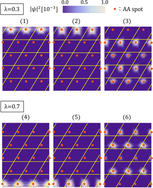
Figure 5 illustrates actual eigenstates of the TBG ribbon, (1), (2) and (3) at $\lambda=0.3$, and (4), (5) and (6) at $\lambda=0.7$, which are labelled in Fig. 4(a). We see that the in-gap states (1) and (2) are actually localized on the upper edge, and (4) and (5) are on the lower edge, while the bulk states (3) and (6) extend over the middle region.

The number of edge states branching out or being absorbed per a sliding cycle ($0\leq\lambda\leq 1$) exactly coincides with the sliding Chern number, which is a topological invariant defined for the Bloch bands of TBG Fujimoto et al. 2020; Zhang et al. 2020; Su and Lin 2020. Let us consider an infinite TBG and assume the Fermi energy lies in an energy gap. When we adiabatically slide the layer $l$ by its own lattice period $\mathbf{a}_{i}^{(l)}$ with the other layer fixed, the change of electronic polarization is written as Fujimoto et al. 2020

Here $u=u_{n\mathbf{k}}(\lambda_{1},\lambda_{2})$ is the eigenstate of the $n$-th band at Bloch wave number $\mathbf{k}$, in the TBG Hamiltonian with the layer $l$ shifted by $\lambda_{1}\mathbf{a}_{1}^{(l)}+\lambda_{2}\mathbf{a}_{2}^{(l)}$. The $k_{j}$ is a dimensionless wave component defined by $\mathbf{k}=k_{1}\mathbf{G}^{M}_{1}+k_{2}\mathbf{G}^{M}_{2}$, where $\mathbf{G}^{M}_{j}$ is the moiré reciprocal lattice vector satisfying $\mathbf{G}^{M}_{i}\cdot\mathbf{L}^{M}_{j}=2\pi\delta_{ij}$. $\Delta\mathbf{P}$ represents the shift of the polarization per a single moiré unit cell area during a sliding cycle .

When the Fermi energy is in the gap just above the flat band, the sliding Chern numbers per spin are calculated as $C_{11}^{(1)}=C_{22}^{(1)}=2$, $C_{11}^{(2)}=C_{22}^{(2)}=-2$ and otherwise 0. Fujimoto et al. 2020 If we slide the layer $2$ by $\Delta\mathbf{x}^{(2)}=(1/2)\mathbf{a}_{1}^{(2)}-\mathbf{a}_{2}^{(2)}$ as considered for the ribbon, the polarization shift per spin becomes

where $\Delta\mathbf{X}$ is the shift of the moiré pattern argued in the previous section. This means that two electrons (per spin) pass through every unit-cell boundary perpendicular to $x$, and it perfectly corresponds the number of the edge states branching out from (or being absorbed to) the flat band per a sliding cycle, as argued in Fig. 4(a).

Figure 4(a) also shows that, in the second gap around 0.8 eV, four bands of the upper edge states go up, and four bands of the lower edge states go down in a sliding process from $\lambda=0$ to 1. Correspondingly, the sliding Chern numbers (per spin) in the gap are $C_{11}^{(1)}=C_{22}^{(1)}=4$, $C_{11}^{(2)}=C_{22}^{(2)}=-4$ and otherwise 0, giving $\Delta\mathbf{P}=4\Delta\mathbf{X}$.

This is analogous to the bulk-edge correspondence for the quantum Hall effect, Hatsugai 1993a; Hatsugai 1993b where a similar transfer of the edge states between energy bands is observed against a change of the Bloch wave number along the ribbon. In the present case, it occurs as a function as a sliding parameter $\lambda$. Unlike the quantum Hall case, the edge states corresponding to the sliding Chern number do not fill out the whole energy gap in a single static physical system with $\lambda$ fixed, but it fills out the gap when $\lambda$ is changed by a cycle. We note that the bulk-edge correspondence for the topological pumping was first proposed for a one-dimensional lattice with time-dependent moving potential. Hatsugai and Fukui 2016

References

- Thouless et al. (1982) D. J. Thouless, M. Kohmoto, M. P. Nightingale, and M. den Nijs, Phys. Rev. Lett. 49, 405 (1982).
- Kane and Mele (2005) C. L. Kane and E. J. Mele, Physical review letters 95, 146802 (2005).
- Qi et al. (2008) X.-L. Qi, T. L. Hughes, and S.-C. Zhang, Physical Review B 78, 195424 (2008).
- Hatsugai (1993a) Y. Hatsugai, Phys. Rev. Lett. 71, 3697 (1993a).
- Hatsugai (1993b) Y. Hatsugai, Phys. Rev. B 48, 11851 (1993b).
- Kohmoto (1985) M. Kohmoto, Annals of Physics 160, 343 (1985).
- Hasan and Kane (2010) M. Z. Hasan and C. L. Kane, Reviews of modern physics 82, 3045 (2010).
- Qi and Zhang (2011) X.-L. Qi and S.-C. Zhang, Reviews of Modern Physics 83, 1057 (2011).
- Kane and Lubensky (2014) C. Kane and T. Lubensky, Nature Physics 10, 39 (2014).
- Kariyado and Hatsugai (2015) T. Kariyado and Y. Hatsugai, Scientific reports 5, 18107 (2015).
- Süsstrunk and Huber (2016) R. Süsstrunk and S. D. Huber, Proceedings of the National Academy of Sciences 113, E4767 (2016).
- Ozawa et al. (2019) T. Ozawa, H. M. Price, A. Amo, N. Goldman, M. Hafezi, L. Lu, M. C. Rechtsman, D. Schuster, J. Simon, O. Zilberberg, and I. Carusotto, Rev. Mod. Phys. 91, 015006 (2019).
- Lu et al. (2014) L. Lu, J. D. Joannopoulos, and M. Soljačić, Nature photonics 8, 821 (2014).
- Lopes dos Santos et al. (2007) J. M. B. Lopes dos Santos, N. M. R. Peres, and A. H. Castro Neto, Phys. Rev. Lett. 99, 256802 (2007).
- Mele (2010) E. J. Mele, Phys. Rev. B 81, 161405 (2010).
- Trambly de Laissardière et al. (2010) G. Trambly de Laissardière, D. Mayou, and L. Magaud, Nano letters 10, 804 (2010).
- Shallcross et al. (2010) S. Shallcross, S. Sharma, E. Kandelaki, and O. A. Pankratov, Phys. Rev. B 81, 165105 (2010).
- Suárez Morell et al. (2010) E. Suárez Morell, J. D. Correa, P. Vargas, M. Pacheco, and Z. Barticevic, Phys. Rev. B 82, 121407 (2010).
- Bistritzer and MacDonald (2011) R. Bistritzer and A. H. MacDonald, Proceedings of the National Academy of Sciences 108, 12233 (2011).
- Kindermann and First (2011) M. Kindermann and P. N. First, Phys. Rev. B 83, 045425 (2011).
- Xian et al. (2011) L. Xian, S. Barraza-Lopez, and M. Y. Chou, Phys. Rev. B 84, 075425 (2011).
- Dos Santos et al. (2012) J. L. Dos Santos, N. Peres, and A. C. Neto, Physical Review B 86, 155449 (2012).
- Moon and Koshino (2012) P. Moon and M. Koshino, Phys. Rev. B 85, 195458 (2012).
- Trambly de Laissardière et al. (2012) G. Trambly de Laissardière, D. Mayou, and L. Magaud, Phys. Rev. B 86, 125413 (2012).
- Moon and Koshino (2013) P. Moon and M. Koshino, Phys. Rev. B 87, 205404 (2013).
- Cao et al. (2016) Y. Cao, J. Y. Luo, V. Fatemi, S. Fang, J. D. Sanchez-Yamagishi, K. Watanabe, T. Taniguchi, E. Kaxiras, and P. Jarillo-Herrero, Phys. Rev. Lett. 117, 116804 (2016).
- Cao et al. (2018a) Y. Cao, V. Fatemi, S. Fang, K. Watanabe, T. Taniguchi, E. Kaxiras, and P. Jarillo-Herrero, Nature 556, 43 (2018a).
- Landgraf et al. (2013) W. Landgraf, S. Shallcross, K. Türschmann, D. Weckbecker, and O. Pankratov, Phys. Rev. B 87, 075433 (2013).
- Suárez Morell et al. (2014) E. Suárez Morell, R. Vergara, M. Pacheco, L. Brey, and L. Chico, Phys. Rev. B 89, 205405 (2014).
- Morell et al. (2015) E. S. Morell, P. Vargas, P. Häberle, S. A. Hevia, and L. Chico, Phys. Rev. B 91, 035441 (2015).
- Pelc et al. (2015) M. Pelc, E. S. Morell, L. Brey, and L. Chico, J. Phys. Chem. C 119, 10076 (2015).
- Fleischmann et al. (2018) M. Fleischmann, R. Gupta, D. Weckbecker, W. Landgraf, O. Pankratov, V. Meded, and S. Shallcross, Physical Review B 97, 205128 (2018).
- Liu et al. (2019) J. Liu, J. Liu, and X. Dai, Physical Review B 99, 155415 (2019).
- Wakabayashi et al. (1999) K. Wakabayashi, M. Fujita, H. Ajiki, and M. Sigrist, Phys. Rev. B 59, 8271 (1999).
- Fujimoto et al. (2020) M. Fujimoto, H. Koschke, and M. Koshino, Phys. Rev. B 101, 041112 (2020).
- Zhang et al. (2020) Y. Zhang, Y. Gao, and D. Xiao, Physical Review B 101, 041410 (2020).
- Su and Lin (2020) Y. Su and S.-Z. Lin, Physical Review B 101, 041113 (2020).
- Thouless (1983) D. J. Thouless, Phys. Rev. B 27, 6083 (1983).
- Nakanishi and Ando (2001) T. Nakanishi and T. Ando, Journal of the Physical Society of Japan 70, 1647 (2001).
- Uryu (2004) S. Uryu, Phys. Rev. B 69, 075402 (2004).
- Slater and Koster (1954) J. C. Slater and G. F. Koster, Phys. Rev. 94, 1498 (1954).
- Cao et al. (2018b) Y. Cao, V. Fatemi, A. Demir, S. Fang, S. L. Tomarken, J. Y. Luo, J. D. Sanchez-Yamagishi, K. Watanabe, T. Taniguchi, E. Kaxiras, et al., Nature 556, 80 (2018b).
- Nam and Koshino (2017) N. N. Nam and M. Koshino, Physical Review B 96, 075311 (2017).
- Koshino et al. (2018) M. Koshino, N. F. Yuan, T. Koretsune, M. Ochi, K. Kuroki, and L. Fu, Physical Review X 8, 031087 (2018).
- Koshino (2015) M. Koshino, New Journal of Physics 17, 015014 (2015).
- Koshino and Moon (2015) M. Koshino and P. Moon, Journal of the Physical Society of Japan 84, 121001 (2015).
- Weckbecker et al. (2016) D. Weckbecker, S. Shallcross, M. Fleischmann, N. Ray, S. Sharma, and O. Pankratov, Physical Review B 93, 035452 (2016).
- Hatsugai and Fukui (2016) Y. Hatsugai and T. Fukui, Physical Review B 94, 041102 (2016).