Geometry effects in the magnetoconductance of normal and Andreev Sinai billiards

Ballistic transport of particles across billiards is a field of major importance due to its fundamental properties as well as physical applications QuaCh; Alha; Ri00; Jalab. In such systems, a two-dimensional cavity is defined by a step-like single-particle potential where confined particles can propagate freely between bounces at the billiard walls. For open systems the possibility of particles being injected and escaping through holes in the boundary is also allowed. As an example, we consider the open geometry of the extensively studied Sinai billiard shown in figure 1. Experimental realizations are based on exploiting the analogy between quantum and wave mechanics in either microwave and acoustic cavities or vibrating plates QuaCh, and on structured two-dimensional electron gases in artificially tailored semiconductor heterostructures Alha; Ri00; Jalab. In the latter case, the particles are also charge carriers making these nanostructures relevant to applied electronics.

Focusing the attention on the electronic analogues, more recently the possibility to couple a superconductor to a ballistic quantum dot has been considered both theoretically KosMasGol; S-billiards and experimentally EPL02ETW, so that some part of the billiard boundary exerts the additional property of Andreev reflection And64. During this process particles with energies much smaller than the superconducting gap are coherently scattered from the superconducting interface as Fermi sea holes back to the normal conducting system (and vice versa). Classically, Andreev reflection manifests itself by retroreflection, i.e., all velocity components are inverted, compared to the specular reflection where only the boundary normal component of the velocity is inverted. Thus, Andreev reflected particles (holes) retrace their trajectories as holes (particles). If, however, a perpendicular magnetic field is applied in addition, such retracing no longer occurs due to the inversion of both the charge and the effective mass of the quasiparticle resulting in opposite bending. Typical trajectories are illustrated in figure 2.

A unique feature of this class of (quantum) mechanical systems is their suitability for studying the quantum-to-classical correspondence. In particular, much effort has been devoted in revealing the quantum fingerprints of the classical dynamics which may be parametrically tuned from regular to chaotic via, e.g., changes in the billiard-shape. A range of theoretical tools has been used, spanning the usual analysis of classical trajectories and the semiclassical approximation to the models of Random Matrix Theory and fully quantum mechanical calculations. The main signatures of classical integrability (or lack of it) on the statistics of energy levels and properties of the transport coefficients for closed and open systems, respectively, have been discussed in detail in various reviews QuaCh; Alha; Ri00; Jalab. Discussions on modifications owing to the possibility of Andreev reflection appear in more recent studies KosMasGol; S-billiards; MBFC96; PRB00CBA; EPJB01ILV; PRL99SB; TA01; PRB04CPP; FTPR05, mostly focusing on the features of the quantum mechanical level density.

The validity of classical calculations of these type of systems has been revealed in reference F05. In fact, it has been shown that a purely classical analysis may provide qualitative rationalization and quantitative predictions for the average quantum mechanical transport properties of a generic billiard, such as the square cavity shape of figure 1, both in the presence or absence of Andreev reflection. Moreover, while in most previous works only the cases of zero or small magnetic field have been considered, in reference F05 the regime of finite magnetic field strengths has been analyzed and it has been shown that the classical trajectories, that depend parametrically on the applied magnetic field, suffice to describe the overall features of the observed non-monotonic behavior. Within this viewpoint, in the present work we study classically the ballistic transport of charge carriers across different geometrical setups originating from the general form of the Sinai-billiard shown in figure 1, under an externally applied magnetic field $B$. We consider four different setups ($W$ is our scaling unit in what follows): (a) a square cavity - centered antidot (sc) setup for which $L_{\rm x}=L_{\rm z}=5W$ and $h=r=W$ ; (b) a square cavity - displaced antidot (sd) setup where the geometric scaling follows setup (a) but now the center of the antidot is displaced at ($r,0$) ; (c) a rectangular cavity - centered antidot (rc) setup where $L_{\rm x}=5W$, $L_{\rm z}=3.75W$, and $h=r=W$ ; and finally (d) a circular cavity - centered antidot (cc) setup with $R=2.5W$ and $h=r=W$ as before. In this particular setup (d) the cavity is shown by the dashed circle in figure 1. In all cases the symmetric leads attached to the left and right side of the cavity define source and sinks of quasiparticles. Note that, the central scattering disk can be either a normal or a superconducting antidot. In the former case the antidot represents an infinitely high potential barrier while in the latter case it is considered as an extended homogeneous superconductor characterized by the property of Andreev reflection KosMasGol. Experimentally, such antidot structures have been realized in periodic arrangements, thus forming superlattices Ri00; EPL02ETW. The boundaries of the square and rectangular cavity, numbered clockwise by the labels 1 through 4 in figure 1, are always normal conducting potential walls of infinite height. The same applies also for the case of the circular cavity, and in particular for the upper and lower semicircles (dashed lines in figure 1).

The general form of the Hamiltonian describing the dynamics of charged particles inside the cavity reads

The index $\alpha$ is used to describe the possibility that the propagating particles are either electrons ($\rm e$) or holes ($\rm h$). This generalization is necessary for a correct description of the dynamics in the setup with the superconducting antidot. The canonical momentum vector is $\vec{p}=(p_{x},p_{z})=m^{*}_{\alpha}\vec{v}+q_{\alpha}\vec{A}$ where $\vec{v}$ is the mechanical velocity, the corresponding position vector being $\vec{r}=(x,z)$. Charge conservation yields $m^{*}_{h}=-m^{*}_{e}$ for the effective masses and $q_{\rm h}=-q_{\rm e}$ for the electric charge. The main property which distinguishes the two cases, i.e., normal/superconducting antidot, is the interaction of the charged particle with the scattering disk. The latter is captured by the elementary processes illustrated in figure 2, namely, specular reflection (SR) versus the Andreev reflection (AR).

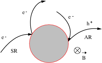
The initial conditions for incoming electrons are determined by the phase-space density $\rho_{o}(x,z,v_{x},v_{z})=\frac{1}{2m^{\ast}_{e}vW}\delta(x+\frac{L}{2})\times\left[\Theta(z+\frac{W}{2})-\Theta(z-\frac{W}{2})\right]\times\delta(m^{*}_{e}(v-v_{F}))\cos\theta$, where $\theta\in[-\frac{\pi}{2},\frac{\pi}{2}]$ is the angle of the initial electron momentum with the $x$-axis and $v_{\rm F}=\sqrt{2E_{\rm F}/m^{\ast}_{\rm e}}$ and the coordinate origin is assumed at the center of the cavity. The trajectories of the charged particles in the billiard consist of segments of circles with cyclotron radius $r=m^{\ast}_{\alpha}v/(-q_{e}B)$ (with $v=\sqrt{v_{x}^{2}+v_{z}^{2}}$). For the magnetic field the symmetric gauge $\vec{A}=[(B/2)z,0,-(B/2)x]$ has been chosen, accounting for a homogeneous magnetic field of strength $B$ in $y$-direction, perpendicular to the two-dimensional system. In what follows, we define as magnetic field unit the value $B_{0}=(m_{\rm e}^{\ast}v_{\rm F})/(-q_{\rm e}W)$ for which the cyclotron radius is equal to $W$. It is convenient to use a dimensionless form of the classical equations of motion by employing the scaling $x=\xi_{x}W$ and $z=\xi_{z}W$ for the spatial coordinates and $t=\tau/\omega$ (with $\omega=B_{0}/m^{*}_{e}$) for the time coordinate. The above quantities are calculated for 100 values of the magnetic field strength varying from 0.01 to 2 using an ensemble of $10^{6}$ different initial conditions distributed according to the phase-space density $\rho_{o}(x,z,v_{x},v_{z})$ given above for each $B$-field value. The magnetic field dependence of typical transmission and reflection coefficients for electrons and holes $T_{\rm e,\rm h}$ and $R_{\rm e,\rm h}$ respectively is shown in figure 3 for the case of the square cavity with a displaced antidot [setup (b) of the Sinai billiard of figure 1] for both a normal and a superconducting (Andreev) version. The obtained curves (similarly also for the other setups) are quite irregular, possibly indicating the presence of fractal fluctuations in the magnetoconductance of the system Ketz, as will also be seen below.

It is known that in the normal case the linear-response low-temperature conductance is simply proportional to the transmission coefficient for electrons $T_{\rm e}$, according to Landauer’s formula $G_{\rm N}=(2e^{2}/h)\;T_{\rm e}$. Lambert et al. Lam93 have worked generalizations for systems including superconducting islands or leads. For the Andreev version of the Sinai billiard system, the conductance is given by $G_{\rm S}=(2e^{2}/h)\;(T_{\rm e}+R_{\rm h})$ where $R_{h}$ is the reflection coefficient for holes. In analogy with the quantum mechanical case, we plot in figure 4 the magnetoconductance of a normal (open circles) and a superconducting (filled stars) antidot for the four setups of the Sinai billiard considered, using the above formulae.

From figure 4 we see that for all the setups considered, with increasing field strength the dependency of the classical trajectories on the applied magnetic field drives the classical dynamics from mixed to regular for both versions of billiards. This is grossly reflected in the non-monotonic behavior of the magnetoconductance, in agreement with the behavior already observed in figure 3 for the transmission and reflection probabilities.

Some general comments are in order: At non vanishing external field the classical dynamics of both the normal and Andreev billiards is characterized by a mixed phase space of coexisting regular and chaotic regions. At $B=0$ the superconducting antidot leads to an integrable dynamics since trajectories are precisely retraced after retroreflection while the corresponding normal device possesses a mixed phase space. There are three families of periodic orbits each forming a continuous set that occur in the classical dynamics and phase space of the closed system Gaspard; Kovacs; Silva, i.e. without leads, leaving their fingerprints in the open system with the attached leads. We will briefly discuss these periodic orbits in the following. At zero field there are orbits bouncing between two opposite walls with velocities parallel to the normal of the corresponding walls. At finite but weak $B$-field strength the periodic orbits form a rosette and incorporate collisions with the antidot and the walls. These periodic orbits are typical, i.e. dominant up to a critical field value $B_{\rm c}$. For magnetic fields above $B_{\rm c}$ the cyclotron radius is so small that no collisions with the antidot can occur and skipping orbits, describing the hopping of the electrons along the billiard walls, become dominant. The values of this critical field $B_{\rm c}$ are marked in the relevant plots by the dotted lines. All periodic orbits possess an eigenvalue one of their stability matrix Fliesser and all periodic orbits possess unstable directions. We remark that the above-discussed periodic orbits of the closed billiard are not trajectories emerging from and ending in the leads of the open billiard. However, trajectories of particles coupled to the leads (i.e., injected and transmitted/reflected) can come close to the periodic orbits of the open billiard thereby tracing their properties. This way the presence of the periodic orbits reflects itself in the transport properties.

Overall, we see that that in the presence of Andreev reflection the conductance of the system is larger than in the normalconducting case for magnetic fields $B<B_{\rm c}$. This holds for the setups (a), (b) and (c) while for the setup (d) we see that $G_{\rm N}\sim G_{\rm S}$. Turning on the superconductivity at the Sinai-billiard disc, the interplay of the bending of the trajectories and the occurring particle-to-hole conversion accounts for a significant increase in the reflection coefficient of holes and therefore for this qualitatively different behavior between the normal and Andreev version of the billiard. On the other hand, setup (d) is an exceptional case, where due to the circular billiard-shape the typical trajectories in the normalconducting case for $B<B_{\rm c}$ give strong contribution to the process of electron transmission. The same orbits, say in setup (a) would contribute to the process of electron reflection, spanning the difference $G_{\rm N}-G_{\rm S}$. For $B>B_{\rm c}$ now, we expect a similar behavior of $G_{\rm N}$ and $G_{\rm S}$ as discussed previously. The small deviation that appears in setup (b) is due to the fact that the interesting feature of the even number of collisions with the antidot which is related to the generic properties of Andreev reflection F05 is destroyed and a small percentage of trajectories showing an odd number of collisions with the circumference of the disc exist, even in the region beyond the critical value of $B$. Setup (c), i.e. the rectangular cavity formed by reducing the z-axis boundary length, gives, as we may see from figure 4, the smaller $G_{\rm N(S)}$ values, with the geometry of this setup being responsible for both the increase in the transmission of holes (and thus the reduction of $G_{\rm S}$) in the superconducting case and the reflection of electrons (and thus the reduction of $G_{N}$) in the corresponding normalconducting case.

We performed simulations of the classical dynamics of low-energy (quasi)particles and identified the magnetoconductance spectrum of four different geometrical setups emerging out of the general geometry of the Sinai billiard shown in figure 1. For each setup, we studied both the normal and Andreev version of the Sinai billiard, i.e. we investigated the interplay between trajectory bending and Andreev reflection and showed how such effects influence the overall (magneto)transport properties of Andreev billiards when compared to their normal counterparts. The classical simulations reported here are not severely demanding in computer time and can be easily tuned according to the parameters defining the setup, i.e. the shape of the cavity, the position/size of the scattering disc and the position/width of the leads. Therefore, we envisage that our study could be further developed and utilized both theoretically and experimentally in future investigations.

References

- (1) K.-F. Berggren, S. Åberg (eds), QUANTUM CHAOS Y2K: Proceedings of Nobel Symposium 116, World Scientific, 2000.
- (2) Y. Alhassid, Rev. Mod. Phys. 72, 895 (2000).
- (3) K. Richter, Semiclassical Theory of Mesoscopic Quantum Systems, in vol. 161 of Springer Tracts in Modern Physics, Springer, Berlin, 2000.
- (4) R.A. Jalabert, in New Directions in Quantum Chaos, edited by G. Casati, I. Guarneri, U. Smilansky, IOS Press, Amsterdam, 2000.
- (5) I. Kosztin, D.L. Maslov, and P.M. Goldbart, Phys. Rev. Lett. 75, 1735 (1995).
- (6) C.W.J. Beenakker, Lect. Notes Phys. 667, 131 (2005).
- (7) J. Eroms, M. Tolkiehn, D. Weiss, U. Rössler, J. DeBoeck, and S. Borghs, Europhys. Lett. 58, 569 (2002).
- (8) A. F. Andreev, JETP 19, 1228 (1964).
- (9) J. Melsen, P. Brouwer, K. Frahm, and C. Beenakker, Europhys. Lett. 35, 7 (1996).
- (10) A.A. Clerk, P. W. Brouwer, and V. Ambegaokar, Phys. Rev. B 62, 10226 (2000).
- (11) W. Ihra, M. Leadbeater, J. L. Vega, and K. Richter, Eur. Phys. J. B 21, 425 (2001).
- (12) H. Schomerus and C.W.J. Beenakker, Phys. Rev. Lett. 82, 2951 (1999).
- (13) D. Taras-Semchuk and A. Altland, Phys. Rev. B 64, 014512 (2001).
- (14) J. Cserti, P. Polinák, G. Palla, U. Zülicke, and C.J. Lambert, Phys. Rev. B 69, 134514 (2004).
- (15) G. Fagas, G. Tkachov, A. Pfund, and K. Richter, Phys. Rev. B 71, 224510 (2005).
- (16) N.G. Fytas, F.K. Diakonos, P. Schmelcher, M. Scheid, A. Lassl, K. Richter, and G. Fagas, Phys. Rev. B 72, 085336 (2005).
- (17) C.J. Lambert, V.C. Hui, and S.J. Robinson, J. Phys. C 5, 4187 (1993).
- (18) A.S. Sachrajda, R. Ketzmerick, C. Gould, Y. Feng, P.J. Kelly, A. Delage, and Z. Wasilewski, Phys. Rev. Lett. 80, 1948 (1998).
- (19) P. Gaspard and J.R. Dorfman, Phys. Rev. E 52, 3525 (1995).
- (20) Z. Kovács, Phys. Rep. 290, 49 (1997).
- (21) L.G.G.V. Dias Da Silva and M. A. M. de Aguiar, Eur. Phys. J. B 16, 719 (2000).
- (22) M. Fliesser, G. J. O. Schmidt, and H. Spohn, Phys. Rev. E 53, 5690 (1996).