Fractonic gauge theory of smectics

A smectic state of matter, is a liquid crystal phase that partially breaks rotational and translational symmetries spontaneously, exhibiting a periodic layered order. Classical smectics form in systems of rod-like constituents (molecules like 5CB) ProstDeGennes; Chaikin2000 and are driven by anisotropic entropic (exclusion volume) interactions. In striking contrast, quantum smectic states appear even in systems of isotropic point-like constituents as a result of frustrated competition between kinetic energy and interactions. In cold atom systems, quantum smectics may be realized in a putative Fulde-Ferrell-Larkin-Ovchinnikov paired superfluidsFF; LO in imbalanced degenerate atomic gases LR_VishwanathPRL; LRpra and in spin-orbit coupled Bose condensates HuiZhai; LR_ChoiPRL. Quantum smectics are also a natural explanation for a striking resistive anisotropy observed in quantum Hall systems at half-filled high Landau levels EisensteinQSm; CsathyARCMP; Fogler; Moessner; FisherMacdonald; LR_Dorsey, and for “striped” spin and charge states of weakly doped correlated quantum magnetsTranquadaStripes; KivelsonStripes.

A two-dimensional (2D) smectic can emerge from partial, anisotropic meltingHalperinOstlund of a crystal, with only one species of dislocations unbinding, such that only one direction of translational symmetry is restored, in a Kosterlitz-Thouless (KT)-like KT phase transition. However, a 2D smectic is unstable to thermal fluctuations, and is always driven into a nematic fluid at any nonzero temperature HalperinOstlund; Landau37; Peierls36; TonerNelson. In contrast, a (2+1)D quantum smectic at zero temperature, is a stable state of matter, whose studies have been limited to a simplest harmonic description, with effects of topological defects and of elastic nonlinearities neglected beyond qualitative discussions (for an exception see Refs. LRpra; Grinstein82; LR2011PRE). This, together with ubiquitous putative realizations provides a strong motivation for the present detailed work, a brief preview of which appeared in a recent publication.Smecticgauge

A complementary motivation for our study is its relation to a new class of topological quantum states of matter – dubbed “fractons” – discovered in theoretical exactly solvable models.Chamon05; Bravyi11; Haah11; Castelnovo12; Yoshida13; Bravyi13; Vijay15; Vijay16 These feature a number of fascinating properties that are believed to lie beyond a conventional quantum field theoretic description.QiAOP2020 The most striking of these are quasiparticles with robust (not just fine-tuned or symmetry imposed) restrictions on their mobility, such as an immobile fracton, and its subdimensional multipoles. Although experimental realizations have been sorely lacking, these theoretical models are intensely studied, motivated by their promise for a robust quantum memoryHaah11 and fundamental interest in a new class of topological quantum liquidsHNreview; AbhinavPremReview.

Following this gapped class of lattice qubit models, fracton-like phenomena were also uncovered in gapless symmetric tensor gauge theories, encoded in a generalized Gauss law, that conserves charge multipoles and thereby constrains mobility of chargesPretko1703; Pretko1707; Slagle. Contemporaneously, a similarity of the constrained dynamics of disclination and dislocation defects in a crystal was conjectured to be dual to charges and dipoles of a gauge theoryRadzihovskyConjectureDuality16. Utilizing a generalization of the familiar XY-to-gauge theory (boson-vortex) dualitydasgupta; fisher, Pretko and RadzihovskyPretkoLRdualityPRL2018 formalized this relation through a duality mapping (explored in other contexts by Zaanen and company Zaanen2017) between a quantum 2D crystal elasticity and a symmetric tensor gauge theory. Under this mapping the stress tensor $\sigma_{ij}$ and momentum vector $\pi_{i}$ fields map onto the electric tensor $E_{ij}$ and magnetic vector $B_{i}$ fields, respectively, with Newton’s law (conservation of momentum) corresponding to Faraday’s law of the tensor gauge theory. Relation of these tensor gauge theories to chiral topological elasticity was also explored in Ref.GromovDualityPRL2019.

This established fracton-elasticity duality allows for numerous predictions for phases and phase transitions of the fracton system, based on the extensive understanding of 2D crystal and their descendent states. For example, different phases of the scalar fracton model - fracton insulator, dipole condensate and fracton condensate, can be regarded as gauge theory counterparts to the “commensurate” and “incommensurate” (supersolid) crystalsPretkoLRsymmetryEnrichedPRL2018; PretkoZhaiLRdualityPRB; Kumar19, hexatic, and isotropic fluid phases of the elasticity theory. The associated finite-temperature dipole-unbinding transition and fracton charge unbinding transition correspond to the classical two-stage melting transitions, i.e., crystal-to-hexatic and hexatic-to-liquid transition respectively.

A complementary and physically more transparent formulation of elasticity-to-fractonic coupled vector gauge theory was recently presentedRadzihovskyHermeleVectorGaugePRL2020. The resulting dual coupled vector gauge theory involves three U(1) vector gauge fields ${\bf A}_{k}$ (with $k=x,y$ denoting flavors) and ${\bf a}$, and their canonically conjugate electric fields ${\bf E}_{k}$ and ${\bf e}$, that encode coupled Goldstone modes, the phonons $u_{k}$ and the local bond angle $\theta$. Building on the treatment of the quantum crystalRadzihovskyHermeleVectorGaugePRL2020 and a recent analysis of the quantum smecticSmecticgauge, we derive and explore extensively the coupled vector gauge theory duality to study the (2+1)D smectic and its quantum phase transitions to a crystal and a nematic, formulated in terms of an array of Higgs transitions. We also utilize it to study 2D and 3D classical smectic and the corresponding classical nematic-to-smectic phase transitions deGennes72; HalperinMa; Helfrich78; NelsonToner; Lubensky81; Grinstein86; Toner82.

In this paper, we develop and explore in detail a dual coupled U(1) vector gauge theory for a 2D quantum smectic, building on a recent study of a 2D quantum crystalRadzihovskyHermeleVectorGaugePRL2020 and a smecticSmecticgauge by one of the authors. The dual description we derive is formulated in terms of two coupled U(1) vector gauge theories, with electric fields $\hat{{\bf E}}$ and $\hat{{\bf e}}$, and canonically conjugate vector potentials $\hat{{\bf A}}$ and $\hat{{\bf a}}$, sourced by dipole and charge current densities, $n_{b},{\bf j}_{b}$ (dislocations) and $n_{s},{\bf j}_{s}$ (disclinations), respectively. The corresponding dual Hamiltonian density is given by

$$\begin{split}\tilde{\mathcal{H}}_{\text{sm}}=&\frac{1}{2}\chi\hat{\bf E}^{2}+\frac{1}{2}\left({\bm{\nabla}}\times\hat{\bf A}\right)^{2}+\frac{1}{2}K\hat{\bf e}^{2}\\ &+\frac{1}{2}\left({\bm{\nabla}}\times\hat{{\bf a}}+\hat{\bf x}\times\hat{\bf A}\right)^{2}-\hat{\bf A}\cdot{\bf j}_{b}-\hat{\bf a}\cdot{\bf j}_{s},\end{split}$$

(1)

supplemented by the generalized Gauss laws,

	$\displaystyle{\bm{\nabla}}\cdot\hat{{\bf E}}$	$\displaystyle=$	$\displaystyle n_{b}+\hat{{\bf e}}\cdot\hat{\bf x},$		(2)
	$\displaystyle{\bm{\nabla}}\cdot\hat{{\bf e}}$	$\displaystyle=$	$\displaystyle n_{s}.$		(3)

We demonstrate that the $n_{s}$ charges (disclinations in the smectic) of this dual gauge theory are subdimensional “lineon”, mobile only transverse to smectic layers (that we take to be along $\hat{\bf x}$), enforced by generalized gauge invariance and associated continuity equation,

$\displaystyle\partial_{t}n_{b}+{\bm{\nabla}}\cdot{\bf j}_{b}$

$\displaystyle=$

$\displaystyle-\hat{\bf x}\cdot{\bf j}.$

(4)

In contrast the dipoles (dislocations) exhibit a finite but highly anisotropically mobility.

Motivated to also understand the quantum crystal-smectic transition, we derive the smectic gauge dual and transition to it by utilizing gauge dual of the quantum crystalRadzihovskyHermeleVectorGaugePRL2020 and condensing one flavor of dipoles (dislocations). The associated Higgs transition gaps out the corresponding flavor of the gauge fields ${\bf A}_{k}$, and leads to a dual quantum smectic Lagrangian, that matches exactly the description obtained through direct duality of smectic elasticity,

$$\tilde{\mathcal{L}}_{\text{sm}}=\frac{1}{2}|\left(\partial_{\mu}+ipA_{\mu}\right)\psi_{x}|^{2}-V\left(|\psi_{x}|\right)+\mathcal{L}_{\text{M}}^{\text{sm}},$$

(5)

where, $\mathcal{L}_{\text{M}}^{\text{sm}}$ is the Maxwell sector from Equation (1), with $V\left(|\psi_{x}|\right)$ a U(1)-invariant Landau potential for $x$-flavor dipoles, $\psi_{x}$. The flow chart in Fig. 1 summarizes these two routes to the dual gauge theory of a quantum smectic.

In this formulation the $\psi_{x}=0$ Coulomb phase corresponds to the quantum smectic phase, and the $\psi_{x}\neq 0$ Higgs phase gives a condensation of unbound $\hat{\bf x}-$dipoles ($\hat{\bf y}-$dislocations) that gaps out the gauge field $A_{\mu}$, which drives a Higgs transition to a quantum nematic. The quantum melting transitions and the corresponding phases are illustrated in Fig. 2.

We also explore the classical limit of this duality, and formulate the 2D smectic-to-nematic melting and a subsequent nematic-to-isotropic fluid transition in terms of a higher-derivative sine-Gordon model,

$$\begin{split}\tilde{\mathcal{H}}_{\text{sm}}=&\frac{1}{2}\chi^{-1}(\partial_{x}^{2}\alpha)^{2}+\frac{1}{2}K^{-1}(\partial_{y}\alpha)^{2}-g_{b}\cos(b\partial_{x}\alpha)\\ &-g_{s}\cos(2\pi\alpha).\end{split}$$

(6)

The first two terms capture the elasticity of a 2D smectic, and the two cosine correspond to dislocations and disclinations, tuned by the corresponding fugacities $g_{b,s}$. We demonstrate that in 2D the dislocations are always relevant, corresponding to the instability of a 2D smectic to a nematic at any nonzero temperature HalperinOstlund; Landau37; Peierls36; TonerNelson. The resulting sine-Gordon model in $\alpha$ then captures the the nematic-to-isotropic fluid transition, illustrated in Fig. 3.

We also derive a classical dual gauge theory for a 3D smectic, that captures its finite-temperature melting into a nematic through a dual normal-superconductor transition with an higher-derivative Maxwell sector, equivalent to Toner’s original treatment of the nematic-to-smectic-A transition.Toner82

The rest of this paper is organized as follows. In Sec. II, after briefly introducing the elasticity theory of a smectic phase and its topological defects, we map a two-dimensional quantum smectic to a dual coupled U(1) vector gauge theory, and use it to demonstrate that its charges (disclinations) exhibit subdimensional constrained mobility. In Sec. III, starting with the coupled U(1) vector gauge theory for a quantum crystal, and “softening” it into a generalized Abelian-Higgs model, we rederive the dual gauge theory of a quantum smectic through a Higgs transition of one flavor of its dipoles. Furthermore, we derive an equivalent low-energy tensor gauge-theory description. In Sec. IV, we explore the classical analogue of these dualities and associated phase transitions, and formulate a higher derivative sine-Gordon model, capturing classical thermal smectic melting transitions. We use it to demonstrate that indeed a 2D smectic is unstable and driven into a nematic at any nonzero temperature. We also generalize this discussion to a 3D classical smectic, and reformulate the 3D nematic to smectic-A transition mediated by unbinding of dislocation loops in terms of a higher-derivative classical normal-superconductor transition. We conclude in Sec. V with a summary of our results and discussion of potential utility of our work.

Ideal smectics are equidistantly layered structures, with a well-defined interlayer spacing $d$, which can be determined through diffraction experiments. With the layers correlations are liquid-like and exhibit crystal-like periodic modulation transverse to the layers, with corresponding density given by,

$$\rho({\bf r})=\rho_{0}+\left(\psi e^{{\bf q}_{0}\cdot{\bf r}}+h.c.\right),$$

(7)

where, ${\bf q}_{0}=\frac{2\pi}{d}\hat{\bf z}$ is the modulation wavevector, and $\psi$ its amplitude, that is the order parameter that distinguishes the smectic phase from the nematic phase.

The deformation of a smectic can be described by its layer displacement field $u({\bf r})$. As the system is invariant under uniform translations, the elastic energy should be expressed purely in terms of derivatives of $u$. Furthermore, the first-order derivatives along the layer, ${\bm{\nabla}}_{\perp}u$, corresponding to merely a uniform rotation of the layers, must cost no energy. Thus, to harmonic order, only the curvature of the layers, ${\bm{\nabla}}_{\perp}^{2}u$, can enter the quadratic part of the elastic energy functional. This point can be seen more explicitly by the following argument. The order parameter $\psi({\bf r})$, describing phonon fluctuations, can be represented as

$$\psi({\bf r})=|\psi|e^{-iq_{0}u({\bf r})},$$

(8)

and the locations of the layer planes can be determined as the constant phase of the molecular density wave,

$$\phi({\bf r})\equiv{\bf q}_{0}\cdot{\bf r}-q_{0}u({\bf r})=2\pi n,n=0,\pm 1,\pm 2,...$$

(9)

The layers local unit-normal is given by,

$$\begin{split}{\bf N}=&\frac{{\bm{\nabla}}\phi}{|{\bm{\nabla}}\phi|}=\frac{\left(-{\bm{\nabla}}_{\perp}u,-\nabla_{\parallel}u,1\right)}{\sqrt{1+\left({\bm{\nabla}}u\right)^{2}}}\\ =&\left(-\partial_{x}u,-\partial_{y}u,1\right)+O[\left({\bm{\nabla}}u\right)^{2}].\end{split}$$

(10)

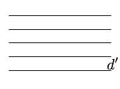
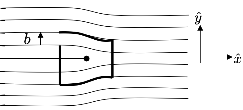
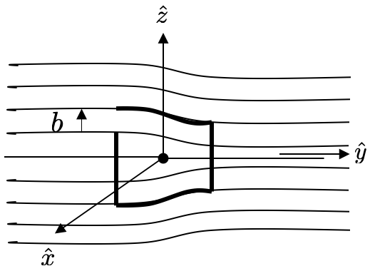
The first-order derivative, ${\bm{\nabla}}_{\perp}u\approx\left(\partial_{x}u,\partial_{y}u,0\right)\approx\hat{\bf z}-{\bf N}$, therefore, corresponds to a rigid rotation of the layers around an axis along the layer plane, and does not contribute to the elastic energy, and, $\nabla_{\parallel}u=\partial_{z}u$, in 3D. (See. Fig.4.)

Consistent with this, the continuum elastic Hamiltonian density for a D-dimensional smectic is given by a well-known expression,

$$\mathcal{H}_{\text{sm}}=\frac{1}{2}\chi\left(\nabla_{\parallel}u\right)^{2}+\frac{1}{2}K\left({\bm{\nabla}}_{\perp}^{2}u\right)^{2},$$

(11)

a Landau-Peierls elastic energy Landau37; Peierls36; LR2011PRE for a one-dimensional solid, where $\chi$ is inverse of the compressional modulus, and $K$ is the bend modulus.

Note that (10) is only correct up to $O[({\bm{\nabla}}u)^{2}]$ for small rotations. For any finite rotations $\theta$,

$$\nabla_{\parallel}u=1-\cos\theta,\;\;\nabla_{\perp}u=-\sin\theta,$$

(12)

and the nonlinear strain, $\nabla_{\parallel}u-\frac{1}{2}({\bm{\nabla}}u)^{2}$, can be straightforwardly seen to be independent of the rotation angle $\theta$. Thus, the rotationally invariant energy density is given by,

$$\mathcal{H}_{\text{sm}}=\frac{1}{2}\chi\left[\nabla_{\parallel}u-\frac{1}{2}({\bm{\nabla}}u)^{2}\right]^{2}+\frac{1}{2}K\left({\bm{\nabla}}_{\perp}^{2}u\right)^{2},$$

(13)

which introduces non-linear elasticity into $\mathcal{H}_{\text{sm}}$, that for $d\leq 3$ leads to a nontrivial anomalous smectic elasticity Grinstein82; LR2011PRE. However, because the focus of our work is on a quantum smectic, these elastic nonlinearities remain irrelevant in (2+1)D and will thus be neglected in the rest of the manuscript.

For the smectic-A phase, the local normal field (layer orientation) ${\bf N}$ and the director field ${\bf n}=\hat{\bf z}+\delta{\bf n}$ are aligned in equilibrium. Thus,

$${\bm{\nabla}}_{\perp}u=-\delta{\bf n},\;\;{\bm{\nabla}}_{\perp}^{2}u=-{\bm{\nabla}}_{\perp}\delta{\bf n}=-{\bm{\nabla}}{\bf n},$$

(14)

and the elastic energy, ignoring nonlinearities, can be represented as

$$\mathcal{H}_{\text{sm}}=\frac{1}{2}\chi\left({\bm{\nabla}}u+\delta{\bf n}\right)^{2}+\frac{1}{2}K\left({\bm{\nabla}}{\bf n}\right)^{2}.$$

(15)

For a 2D smectic, with the layers along $\hat{\bf x}$ (with layer normal along $\hat{\bf y}$), the elastic Hamiltonian density in Eq.(11) reduces to

$$\mathcal{H}_{\text{sm}}=\frac{1}{2}\chi\left(\partial_{y}u\right)^{2}+\frac{1}{2}K\left(\partial_{x}^{2}u\right)^{2},$$

(16)

where the layer displacement $u$ is along the $\hat{\bf y}$ axis, and the layer orientation (director field) is, ${\bf n}=-\hat{\bf x}\sin\theta+\hat{\bf y}\cos\theta=\hat{\bf y}+\delta{\bf n}$.

Another way to obtain smectic elasticity is to start out with a elasticity of a 2D crystal and allow nonsingle-valued displacement field $u_{x}$, with ${\bm{\nabla}}u_{x}={\bf v}_{x}$, accounting for a plasma of unbound dislocations with Burgers vector along the $\hat{\bf x}-$directed smectic layers, where ${\bf v}_{x}$ is an arbitrary vector with $\epsilon_{ij}\partial_{i}v_{jx}=b_{x}$. Integrating over strain tensor field ${\bf v}_{x}$, leads to the smectic harmonic elasticity,

$$\begin{split}\mathcal{H}_{\text{sm}}=&\mathcal{H}_{\text{cr+disl.}}=\mu u_{ij}^{2}+\frac{1}{2}\lambda u_{ii}^{2}\\ =&\mu\left(u_{xx}^{2}+u_{yy}^{2}+2u_{xy}^{2}\right)+\frac{1}{2}\lambda\left(u_{xx}+u_{yy}\right)^{2}+\frac{1}{2}E_{c}b_{x}^{2}\\ =&\mu\left[v_{xx}^{2}+\left(\partial_{y}u_{y}\right)^{2}+\frac{1}{2}\left(\partial_{x}u_{y}+v_{yx}\right)^{2}\right]\\ &+\frac{1}{2}\lambda\left(v_{xx}+u_{yy}\right)^{2}+\frac{1}{2}E_{c}\left(\partial_{x}v_{yx}-\partial_{y}v_{xx}\right)^{2}\\ =&\frac{1}{2}\chi\left(\partial_{y}u_{y}\right)^{2}+\frac{1}{2}K\left(\partial_{x}^{2}u_{y}\right)^{2},\end{split}$$

(17)

where compressional modulus is $\chi=4\mu(\mu+\lambda)/(2\mu+\lambda)$, bend modulus $K=E_{c}$, and higher derivative terms are neglected after integrating out the ${\bf v}_{x}$ field in the last step.

Equivalently, the smectic elasticity can be formulated in terms of the orientational (nematic) angle degree of freedom $\theta$, which corresponds to the orientation of the layers, with the elastic Hamiltonian density given by,

$$\mathcal{H}_{\text{sm}}=\frac{1}{2}\chi\left({\bm{\nabla}}u-\theta\hat{\bf x}\right)^{2}+\frac{1}{2}K\left({\bm{\nabla}}\theta\right)^{2}.$$

(18)

At low energies set by $\chi$, this Hamiltonian reduces to the conventional form (16) after Higgs’ing out the bond angle $\theta$, locking $\partial_{x}u=\theta$.

Classical elastic Hamiltonian in (18) is easily generalized to a quantum smectic by elevating $u$ and $\theta$ to operators, and adding canonically conjugate linear and angular momenta operators, $\hat{\pi}$ and $\hat{L}$, respectively. This gives,

$$\hat{\mathcal{H}}_{\text{sm}}=\frac{1}{2}\hat{\bf\pi}^{2}+\frac{1}{2}\hat{L}^{2}+\frac{1}{2}\chi\left({\bm{\nabla}}\hat{u}-\hat{\theta}\hat{\bf x}\right)^{2}+\frac{1}{2}K\left({\bm{\nabla}}\hat{\theta}\right)^{2},$$

(19)

for bosonic smectic supplemented with canonical commutation relations ($\hbar=1$),

	$\displaystyle\left[\hat{u}({\bf r}),\hat{\pi}({\bf r}^{\prime})\right]$	$\displaystyle=$	$\displaystyle i\delta^{2}\left({\bf r}-{\bf r}^{\prime}\right),$		(20a)
	$\displaystyle\left[\hat{\theta}({\bf r}),\hat{L}({\bf r}^{\prime})\right]$	$\displaystyle=$	$\displaystyle i\delta^{2}\left({\bf r}-{\bf r}^{\prime}\right).$		(20b)

It is convenient to work with a path-integral formulation where quantum nature of these fields is accounted for by functional integration in phase-space of these fields. We consider the evolution operator for the quantum smectic,

$$U(u^{\prime},\theta^{\prime},u,\theta;t)=\langle u^{\prime},\theta^{\prime}|e^{-i\int_{{\bf r}}\hat{\mathcal{H}}_{\text{sm}}t}|u,\theta\rangle,$$

(21)

and rewrite it in phase-space functional integral formulation as,

$$\begin{split}U&=\int\left[du\right]\left[d\pi\right]\left[d\theta\right]\left[dL\right]e^{iS_{\text{sm}}}\\ &=\int\left[du\right]\left[d\pi\right]\left[d\theta\right]\left[dL\right]e^{i\int dt\int_{{\bf r}}\mathcal{L}_{\text{sm}}},\end{split}$$

(22)

with the corresponding Lagrangian density given by,

$$\begin{split}\mathcal{L}_{\text{sm}}=&\pi\partial_{t}u+L\partial_{t}\theta-\frac{1}{2}\pi^{2}-\frac{1}{2}L^{2}+\frac{1}{2}\chi^{-1}{\bf\sigma}^{2}+\frac{1}{2}K^{-1}{{\bf j}}^{2}\\ &-{\bf\sigma}\cdot\left({\bm{\nabla}}u-\theta\hat{\bf x}\right)-{{\bf j}}\cdot{\bm{\nabla}}\theta.\end{split}$$

(23)

In addition to the single-valued (smooth) Goldstone mode degrees of freedom, $\tilde{\theta}$ and $\tilde{u}$, we must also include topological defects – disclinations and dislocations, captured by including a nonsingle-valued component of the bond angle field $\theta^{s}$ and of the phonon distortion field $u^{s}$, respectively. In the smectic, a disclination at a point ${\bf r}_{0}$, is defined by a nonzero closed line-integral of the gradient of the bond angle around ${\bf r}_{0}$, $\oint_{{\bf r}_{0}}d\theta=2\pi n_{s}$, or equivalently in a differential form,

$$\hat{\bf z}\cdot{\bm{\nabla}}\times{\bm{\nabla}}\theta^{s}=2\pi n_{s}\delta^{2}({\bf r}-{\bf r}_{0})\equiv n_{s}({\bf r}),$$

(24)

measuring the deficit/surplus bond angle. $n_{s}({\bf r})$ is the disclination charge density. A disclination with charge $n_{s}=-\frac{1}{2}$, and a disclination with charge $n_{s}=+\frac{1}{2}$ are illustrated in Fig. 5(a, b).

A dislocation at ${\bf r}_{0}$ with a Burgers charge $n_{b}$ (that is an integer multiples of the elementary layer spacing), is defined by a closed line-integral, $\oint_{{\bf r}_{0}}du=n_{b}$, or equivalently in the differential form,

$$\hat{\bf z}\cdot{\bm{\nabla}}\times{\bm{\nabla}}u^{s}=n_{b}\delta^{2}({\bf r}-{\bf r}_{0})\equiv n_{b}({\bf r}),$$

(25)

where $n_{b}({\bf r})$ is the Burgers charge density. A dislocation in the smectic is shown in Fig. 5(c), which can be regarded as a tightly bound pair of $+\frac{1}{2}$ and $-\frac{1}{2}$ disclinations.

In anticipation of our more rigorous duality derivation, already here we can argue for the subdimensional nature of the disclination dynamics in a smectic. Consider a pair of oppositely charged $\pm\frac{1}{2}$ disclinations separated along $\hat{x}$ axis, as shown in Fig. 6. The separation between the pair is large such that we can regard them as isolated disclinations. Moving the ‘$+$’ disclination along the layers (i.e., $\hat{\bf x}$ axis) by two layer spacings, requires the introduction of four extra half-layers of molecules, which is a highly non-local process in terms of atoms quantum dynamics, and is therefore not allowed. While moving the ‘$+$’ disclination transversely (i.e., in $\hat{y}$ direction) preserves the strength of the dislocation, and thus, is allowed dynamically, even though there is an energy cost for separating the ‘$+$’ and ‘$-$’ disclination pair that make up the dislocation. Similar analysis applies to the ‘$-$’ disclination. Thus, we conclude that disclinations can only move transversely to the layers, i.e., they manifests the subdimensional lineon dynamics.

To include the topological defects in the complete description of the smectic, we decompose the distortion field $u$ and the bond angle $\theta$ into the smooth elastic and nonsingle-valued components,

$$u=\tilde{u}+u^{s},\ \ \theta=\tilde{\theta}+\theta^{s}.$$

(26)

Integrating out the single-valued parts $\tilde{u}$ and $\tilde{\theta}$ out of the total generating function,

$$U=\int\left[d\tilde{u}\right][d\tilde{\theta}]\left[du^{s}\right]\left[d\pi\right]\left[d\theta^{s}\right]\left[dL\right]e^{i\int dt\int_{{\bf r}}\mathcal{L}_{\text{sm}}},$$

(27)

leads to,

$$U=\int\left[du^{s}\right]\left[d\pi\right]\left[d\theta^{s}\right]\left[dL\right]e^{i\int dt\int_{{\bf r}}\mathcal{L}_{\text{sm}}},$$

(28)

where the new Lagrangian density is given in terms of only nonsingular components,

$$\begin{split}\mathcal{L}_{\text{sm}}=&\pi\partial_{t}u^{s}+L\partial_{t}\theta^{s}-\frac{1}{2}\pi^{2}-\frac{1}{2}L^{2}+\frac{1}{2}\chi^{-1}{\bf\sigma}^{2}\\ &-{\bf\sigma}\cdot\left({\bm{\nabla}}u^{s}-\theta^{s}\hat{\bf x}\right)+\frac{1}{2}K^{-1}{{\bf j}}^{2}-{{\bf j}}\cdot{\bm{\nabla}}\theta^{s},\end{split}$$

(29)

with two enforced constraints,

	$\displaystyle\partial_{t}\pi-{\bm{\nabla}}\cdot{\bf\sigma}\equiv\partial_{\mu}J_{\mu}=0,$		(30)
	$\displaystyle\partial_{t}L-{\bm{\nabla}}\cdot{\bf j}-\sigma_{x}=0,$		(31)

where we implicitly introduced currents $J_{\mu}=\left(\pi,-\sigma_{i}\right)$.

The momentum continuity equation (30) can be solved in terms of gauge potential fields, $A_{\mu}$, with

$$J_{\mu}=\epsilon_{\mu\nu\gamma}\partial_{\nu}A_{\gamma}=\left(\epsilon_{ij}\partial_{i}A_{j},\epsilon_{i\nu\gamma}\partial_{\nu}A_{\gamma}\right),$$

(32)

such that

	$\displaystyle\pi=\epsilon_{ij}\partial_{i}A_{j}=\hat{\bf z}\cdot\left({\bm{\nabla}}\times{\bf A}\right),$		(33)
	$\displaystyle\sigma_{i}=-\epsilon_{i\nu\gamma}\partial_{\nu}A_{\gamma}=\epsilon_{ij}(\partial_{t}A_{j}-\partial_{j}A_{0}),$		(34)

and Eq.(31) transforms into

$$\partial_{t}\left(L-\epsilon_{xj}A_{j}\right)-\partial_{i}\left(j_{i}-\epsilon_{xi}A_{0}\right)\equiv\partial_{\mu}\tilde{j}_{\mu}=0,$$

(35)

with $\tilde{j}_{\mu}=\left(L-\epsilon_{xj}A_{j},-j_{i}+\epsilon_{xi}A_{0}\right)$, which is then solved by introducing another vector gauge potential $a_{\mu}$,

$$\tilde{j}_{\mu}=\epsilon_{\mu\nu\gamma}\partial_{\nu}a_{\gamma},$$

(36)

such that

	$\displaystyle L$	$\displaystyle=$	$\displaystyle\epsilon_{ij}\partial_{i}a_{j}+\epsilon_{xj}A_{j}=\hat{\bf z}\cdot\left({\bm{\nabla}}\times{\bf a}+\hat{\bf x}\times{\bf A}\right),$		(37)
	$\displaystyle j_{i}$	$\displaystyle=$	$\displaystyle\epsilon_{ij}(\partial_{t}a_{j}-\partial_{j}a_{0})+\epsilon_{xi}A_{0}.$		(38)

Substituting the solutions of $\pi,\sigma_{i},L$,and $j_{i}$ in terms of the gauge fields into the Lagrangian density, leads to the dual Lagrangian density

$$\tilde{\mathcal{L}}_{\text{sm}}=\mathcal{L}_{\text{M}}^{\text{sm}}+{\bf A}\cdot{\bf j}^{b}+A_{0}n_{b}+{\bf a}\cdot{\bf j}^{s}+a_{0}n_{s},$$

(39)

where $\mathcal{L}_{\text{M}}$ is the Maxwell part, given by

$$\begin{split}\mathcal{L}_{\text{M}}^{\text{sm}}=&\frac{1}{2}\chi^{-1}\left(\partial_{t}{\bf A}-{\bm{\nabla}}A_{0}\right)^{2}-\frac{1}{2}\left({\bm{\nabla}}\times{\bf A}\right)^{2}\\ &+\frac{1}{2}K^{-1}\left(\partial_{t}{\bf a}-{\bm{\nabla}}a_{0}-A_{0}\hat{\bf x}\right)^{2}-\frac{1}{2}\left({\bm{\nabla}}\times{\bf a}+\hat{\bf x}\times{\bf A}\right)^{2},\end{split}$$

(40)

and the charge contributions are obtained by integrating by parts and defining the dislocation and disclination charge and current densities as,

	$\displaystyle n_{b}$	$\displaystyle=$	$\displaystyle\epsilon_{ij}\partial_{i}\partial_{j}u,$		(41a)
	$\displaystyle n_{s}$	$\displaystyle=$	$\displaystyle\epsilon_{ij}\partial_{i}\partial_{j}\theta,$		(41b)
	$\displaystyle j^{b}_{i}$	$\displaystyle=$	$\displaystyle\epsilon_{ij}\left(\partial_{j}\partial_{t}u-\partial_{t}\partial_{j}u\right),$		(41c)
	$\displaystyle j^{s}_{i}$	$\displaystyle=$	$\displaystyle\epsilon_{ij}\left(\partial_{j}\partial_{t}\theta-\partial_{t}\partial_{j}\theta\right).$		(41d)

Introducing Hubbard-Stratonovich fields ${\bf E}$ and ${\bf e}$, the Lagrangian density transforms into

$$\begin{split}\tilde{\mathcal{L}}_{\text{sm}}=&-{\bf E}\cdot\left(\partial_{t}{\bf A}-{\bm{\nabla}}A_{0}\right)-\frac{1}{2}\chi{\bf E}^{2}-\frac{1}{2}\left({\bm{\nabla}}\times{\bf A}\right)^{2}-\frac{1}{2}K{\bf e}^{2}\\ &-{\bf e}\cdot\left(\partial_{t}{\bf a}-{\bm{\nabla}}a_{0}-A_{0}\hat{\bf x}\right)-\frac{1}{2}\left({\bm{\nabla}}\times{\bf a}+\hat{\bf x}\times{\bf A}\right)^{2}\\ &+{\bf A}\cdot{\bf j}^{b}+A_{0}n_{b}+{\bf a}\cdot{\bf j}^{s}+a_{0}n_{s}.\end{split}$$

(42)

Integrating over $A_{0}$ and $a_{0}$ gives the Gauss law, leaving the standard Lagrangian form, $\tilde{\mathcal{L}}_{\text{sm}}=-{\bf E}\cdot\partial_{t}{\bf A}-{\bf e}\cdot\partial_{t}{\bf a}-\tilde{\mathcal{H}}_{\text{sm}}$, from which we can read off the dual Hamiltonian density, that is given by,

$$\begin{split}\tilde{\mathcal{H}}_{\text{sm}}=&\frac{1}{2}\chi{\hat{\bf E}}^{2}+\frac{1}{2}\left({\bm{\nabla}}\times{\hat{\bf A}}\right)^{2}+\frac{1}{2}K{\hat{\bf e}}^{2}\\ &+\frac{1}{2}\left({\bm{\nabla}}\times{\hat{{\bf a}}}+\hat{\bf x}\times{\hat{\bf A}}\right)^{2}-{\hat{\bf A}}\cdot{\bf j}^{b}-\hat{\bf a}\cdot{\bf j}^{s},\end{split}$$

(43)

supplemented by the generalized Gauss laws

	$\displaystyle{\bm{\nabla}}\cdot\hat{\bf E}$	$\displaystyle=$	$\displaystyle n_{b}+\hat{\bf e}\cdot\hat{\bf x},$		(44)
	$\displaystyle{\bm{\nabla}}\cdot\hat{\bf e}$	$\displaystyle=$	$\displaystyle n_{s},$		(45)

where, ${\bf E}$ and ${\bf e}$, are independent electric fields, canonically conjugate to the corresponding vector potentials, ${\bf A}$ and ${\bf a}$, respectively.

The above Hamiltonian must be invariant under the gauge transformations:

	$\displaystyle(A_{0},A_{i})\to A_{\mu}^{\prime}=\left(A_{0}+\partial_{t}\chi,(A_{i}+\partial_{i}\chi)\right),$		(46a)
	$\displaystyle(a_{0},a_{i})\to a_{\mu}^{\prime}=\left(a_{0}+\partial_{t}\phi,(a_{i}+\partial_{i}\phi+\hat{\bf x}_{i}\chi)\right).\;\;\;\;\;\;\;$		(46b)

Requiring the source term to preserve this gauge invariance, we obtain coupled continuity equations for charges (disclinations) and dipoles (dislocations), satisfying,

	$\displaystyle\partial_{t}n_{s}+{\bm{\nabla}}\cdot{\bf j}_{s}$	$\displaystyle=$	$\displaystyle 0,$		(47)
	$\displaystyle\partial_{t}n_{b}+{\bm{\nabla}}\cdot{\bf j}_{b}$	$\displaystyle=$	$\displaystyle-j_{s}^{x}.$		(48)

We observe that the dipole (dislocation) continuity equation is violated by a nonzero charge (disclination) current $j_{s}^{x}$ in the $\hat{\bf x}$ (along the layers) direction. Thus, in the absence of gapped $\hat{\bf x}-$dipoles ($\hat{\bf y}$-dislocations), we find that $j_{s}^{x}=0$, i.e., motion of isolated fracton charges (disclinations) is restricted to be transverse to the smectic layers, as moving along the layers requires $\hat{\bf x}$-dipoles ($\hat{\bf y}$-dislocations) that are gapped in the smectic. Therefore, the fractons (disclinations) exhibit subdimensional lineon dynamics, as argued in Section II.2.

References

- (1) P. G. de Gennes and J. Prost, The Physics of Liquid Crystals, 2nd Edition. Clarendon Press, Oxford (1993).
- (2) P. M. Chaikin and T. C. Lubensky, Principles of Condensed Matter Physics. Cambridge University Press (2000).
- (3) P. Fulde and R.A. Ferrell, Superconductivity in a Strong Spin-Exchange Field, Phys. Rev. 135, A550 (1964).
- (4) A.I. Larkin and Yu. N. Ovchinnikov, Nonuniform state of superconductors, Sov. Phys. JETP 20, 762 (1965).
- (5) L. Radzihovsky and A. Vishwanath, Quantum Liquid Crystals in an Imbalanced Fermi Gas: Fluctuations and Fractional Vortices in Larkin-Ovchinnikov States, Phys. Rev. Lett. 103, 010404, (2009).
- (6) L. Radzihovsky, Fluctuations and phase transitions in Larkin-Ovchinnikov liquid-crystal states of a population-imbalanced resonant Fermi gas, Phys. Rev. A. 84, 023611 (2011).
- (7) Hui Zhai, Degenerate quantum gases with spin-orbit coupling: a review, Rep. Prog. Phys. 78, 026001 (2015).
- (8) L. Radzihovsky and S. Choi, p-Wave Resonant Bose Gas: A Finite-Momentum Spinor Superfluid, Phys. Rev. Lett. 103, 095302 (2009).
- (9) M. P. Lilly, K. B. Cooper, J. P. Eisenstein, L. N. Pfeiffer, and K. W. West, Evidence for an Anisotropic State of Two-Dimensional Electrons in High Landau Levels, Phys. Rev. Lett. 82, 394 (1999).
- (10) K. A. Schreiber and G. A. Csáthy, Competition of pairing and nematicity in the two-dimensional electron gas Ann. Rev. Cond. Mat. Phys. 11, 17 (2020).
- (11) A. A. Koulakov, M. M. Fogler, and B. I. Shklovskii, Charge Density Wave in Two-Dimensional Electron Liquid in Weak Magnetic Field, Phys. Rev. Lett. 76, 499 (1996).
- (12) R. Moessner and J. T. Chalker, Exact results for interacting electrons in high Landau levels, Phys. Rev. B 54, 5006 (1996).
- (13) Emiliano Papa, John Schliemann, A. H. MacDonald, and Matthew P. A. Fisher, Quantum theory of bilayer quantum Hall smectics, Phys. Rev. B 67, 115330 (2003).
- (14) L. Radzihovsky and A. T. Dorsey, Theory of Quantum Hall Nematics, Phys. Rev. Lett. 88, 216802 (2002).
- (15) J. M. Tranquada, et. el., Coexistence of, and competition between, superconductivity and charge-stripe order in LaNdSrCuO, Phys. Rev. Lett. 78, 338 (1997).
- (16) S. A. Kivelson, E. Fradkin, V. J. Emery, Electronic liquid crystal phases of a doped Mott insulator, Nature 393, 550-553 (1998).
- (17) S. Ostlund and B. I. Halperin, Dislocation-mediated melting of anisotropic layers, Phys. Rev. B 23, 335 (1981).
- (18) J. M. Kosterlitz and D. J. Thouless, Ordering, metastability and phase transitions in two-dimensional systems, J. Phys. C 6, 1181 (1972).
- (19) L. D. Landau, On the theory of phase transition, Phys. Z. Sowjetunion II, 26 (1937). [Eng. trans.: Collected papers of L.D. Landau, ed. D. ter Haar (Gordon and Breach, New York, 1965), pp. 193-217].
- (20) R. Peierls, Helv. Phys. Acta., Suppl. II 7, 81 (1936).
- (21) John Toner and David R. Nelson, Smectic, cholesteric, and Rayleigh-Benard order in two dimensions, Phys. Rev. B 23, 316 (1981).
- (22) G. Grinstein and Robert A. Pelcovits, Nonlinear elastic theory of smectic liquid crystals, Phys. Rev. A 26, 915 (1982).
- (23) L. Radzihovsky and T. C. Lubensky, Nonlinear smectic elasticity of helical state in cholesteric liquid crystals and helimagnets, Phys. Rev. E 83, 051701 (2011).
- (24) L. Radzihovsky, Quantum smectic gauge theory, arXiv:2009.06632 [cond-mat.str-el], Phys. Rev. Lett. 125, 267601 (2020).
- (25) C. Chamon, Quantum Glassiness in Strongly Correlated Clean Systems: An Example of Topological Overprotection, Phys. Rev. Lett. 94, 040402 (2005).
- (26) S. Bravyi, B. Leemhuis, and B. M. Terhal, Topological order in an exactly solvable 3D spin model, Ann. Phys. (Amsterdam) 326, 839 (2011).
- (27) J. Haah, Local stabilizer codes in three dimensions without string logical operators, Phys. Rev. A 83, 042330 (2011).
- (28) C. Castelnovo and C. Chamon, Topological quantum glassiness, Philos. Mag. 92, 304 (2012).
- (29) B. Yoshida, Exotic topological order in fractal spin liquids, Phys. Rev. B 88, 125122 (2013).
- (30) S. Bravyi and J. Haah, Quantum Self-Correction in the 3D Cubic Code Model, Phys. Rev. Lett. 111, 200501 (2013).
- (31) S. Vijay, J. Haah, and L. Fu, A new kind of topological quantum order: A dimensional hierarchy of quasiparticles built from stationary excitations, Phys. Rev. B 92, 235136 (2015).
- (32) S. Vijay, J. Haah, and L. Fu, Fracton topological order, generalized lattice gauge theory and duality, Phys. Rev. B 94, 235157 (2016).
- (33) M. Qi, L. Radzihovsky, and M. Hermele, Fracton phases via exotic higher-form symmetry-breaking, Annals of Physics, 168360 (2020).
- (34) R. M. Nandkishore and M. Hermele, Fractons, Annu. Rev. Condens. Matter Phys. 10, 295 (2019).
- (35) Abhinav Prem, Michael Pretko, and Rahul M. Nandkishore, Emergent phases of fractonic matter, Phys. Rev. B 97, 085116 (2018).
- (36) M. Pretko, Subdimensional particle structure of higher rank U(1) spin liquids, Phys. Rev. B 95, 115139 (2017).
- (37) M. Pretko, Generalized electromagnetism of subdimen- sional particles, Phys. Rev. B 96, 035119 (2017).
- (38) K. Slagle and Y. B. Kim, Fracton topological order from nearest-neighbor two-spin interactions and dualities, Phys. Rev. B 96, 165106 (2017).
- (39) L. Radzihovsky, unpublished (2016).
- (40) C. Dasgupta and B. I. Halperin, Phase transition in a lattice model of superconductivity, Phys. Rev. Lett. 47, 1556 (1981).
- (41) M. P. A. Fisher and D. H. Lee, Correspondence between two-dimensional bosons and a bulk superconductor in a magnetic field, Phys. Rev. B 39, 2756 (1989).
- (42) M. Pretko and L. Radzihovsky, Fracton-elasticity duality, Phys. Rev. Lett. 120, 195301 (2018).
- (43) J. Beekman, J. Nissinen, K. Wu, K. Liu, R.-J. Slager, Z. Nussinov, V. Cvetkovic, and J. Zaanen, Dual gauge field theory of quantum liquid crystals in two dimensions, Phys. Rep. 683, 1 (2017).
- (44) Andrey Gromov, Chiral Topological Elasticity and Fracton Order, Phys. Rev. Lett. 122, 076403 (2019).
- (45) M. Pretko and L. Radzihovsky, Symmetry-Enriched Fracton Phases from Supersolid Duality, Phys. Rev. Lett. 121, 235301 (2018).
- (46) M Pretko, Z Zhai and L Radzihovsky, Crystal-to-fracton tensor gauge theory dualities, Phys. Rev. B 100, 134113 (2019).
- (47) Ajesh Kumar and Andrew C. Potter, Symmetry-enforced fractonicity and two-dimensional quantum crystal melting, Phys. Rev. B 100, 045119 (2019).
- (48) L. Radzihovsky and M. Hermele, Fractons from vector gauge theory, Phys. Rev. Lett. 124, 050402 (2020).
- (49) D. L. Stein, Kosterlitz-Thouless phase transitions in two-dimensional liquid crystals, Phys. Rev. B 18, 2397 (1978); D. R. Nelson and J. M. Kosterlitz, Universal Jump in the Superfluid Density of Two-Dimensional Superfluids, Phys. Rev. Lett. 39, 1201 (1977).
- (50) P. G. DeGennes, An analogy between superconductors and smectics A, Solid State Commun. 10, 753 (1972).
- (51) B. I. Halperin, T. C. Lubensky, and S. K. Ma, First-Order Phase Transitions in Superconductors and Smectic- A Liquid Crystals, Phys. Rev. Lett. 32, 292 (1974).
- (52) W. Helfrich, Defect model of the smectic A-nematic phase transition, J. Phys. (Paris) 39, 1199 (1978).
- (53) D. R. Nelson and J. Toner, Bond-orientational order, dislocation loops, and melting of solids and smectic-A liquid crystals, Phys. Rev. B 24, 363 (1981).
- (54) T. C. Lubensky, S. G. Dunn, and Joel Isaacson, Gauge Transformations and the Nematic to Smectic-A Transition, Phys. Rev. Lett. 47, 1609 (1981).
- (55) G. Grinstein, T. C. Lubensky, and J. Toner, Defect-mediated melting and new phases in three-dimensional systems with a single soft direction, Phys. Rev. B 33, 3306 (1986).
- (56) J. Toner, Renormalization-group treatment of the dislocation loop model of the smectic-A-nematic transition, Phys. Rev. B 26, 462 (1982).
- (57) M. C. Marchetti and L. Radzihovsky, Interstitials, vacancies and dislocations in flux-line lattices: A theory of vortex crystals, supersolids and liquids. Phys. Rev. B 59, 12001 (1999), arXiv:cond-mat/9811193v2.
- (58) D. R. Nelson and B. I. Halperin, Dislocation-mediated melting in two dimensions, Phys. Rev. B 19, 2457 (1979).
- (59) B. I. Halperin, Superfluidity, melting and liquid-crystal phases in two dimensions, in Proceeding of Kyoto Summer Institute 1979- Physics of Low Dimensional Systems, edited by Y. Nagaoka and S. Hikami (Publications Office, Progress of Theoretical Physics, Kyoto, 1979).
- (60) J. V. José, L. P. Kadanoff, S. Kirkpatrick, and D. R. Nelson, Renormalization, vortices, and symmetry-breaking perturbations in the two-dimensional planar model, Phys. Rev. B 16, 1217 (1977).
- (61) Z. Zhai and L. Radzihovsky, Two-dimensional melting via sine-Gordon duality, Phys. Rev. B 100, 094105 (2019).