跳到论文正文
W Papers独立论文阅读器 arXiv:2012.01929 论文正文 计算阅读时间 · 0%
引用这篇论文根据当前论文元数据生成,正式投稿前建议核对。


License: arXiv.org perpetual non-exclusive license
arXiv:2012.01929v1 [cs.LG] 30 Nov 2020

A Stochastic Path-Integrated Differential EstimatoR Expectation Maximization Algorithm

Gersende Fort Affiliation: Institut de Mathématiques de Toulouse Affiliation: Université de Toulouse; CNRS Affiliation: UPS, Toulouse, France Email: gersende.fort@math.univ-toulouse.fr    Eric Moulines Affiliation: Centre de Mathématiques Appliquées Affiliation: Ecole Polytechnique, France Affiliation: CS Dpt, HSE University, Russian Federation Email: eric.moulines@polytechnique.edu    Hoi-To Wai Affiliation: Department of SEEM Affiliation: The Chinese University of Hong Kong Affiliation: Shatin, Hong Kong Email: htwai@cuhk.edu.hk
Abstract

The Expectation Maximization (EM) algorithm is of key importance for inference in latent variable models including mixture of regressors and experts, missing observations. This paper introduces a novel EM algorithm, called SPIDER-EM, for inference from a training set of size nn, n≫1n\gg 1. At the core of our algorithm is an estimator of the full conditional expectation in the E-step, adapted from the stochastic path-integrated differential estimator (SPIDER) technique. We derive finite-time complexity bounds for smooth non-convex likelihood: we show that for convergence to an ϵ\epsilon-approximate stationary point, the complexity scales as KOpt​(n,ϵ)=𝒪⁡(ϵ−1)K_{\operatorname{Opt}}(n,\epsilon)={\cal O}(\epsilon^{-1}) and KCE​(n,ϵ)=n+n​𝒪​(ϵ−1)K_{\operatorname{CE}}(n,\epsilon)=n+\sqrt{n}{\cal O}(\epsilon^{-1}), where KOpt​(n,ϵ)K_{\operatorname{Opt}}(n,\epsilon) and KCE​(n,ϵ)K_{\operatorname{CE}}(n,\epsilon) are respectively the number of M-steps and the number of per-sample conditional expectations evaluations. This improves over the state-of-the-art algorithms. Numerical results support our findings.


This paper is close to the final version accepted for publication in the Conference on Neural Information Processing Systems (NeurIPS 2020). The final version can be found at
https://papers.nips.cc/paper/2020/hash/c589c3a8f99401b24b9380e86d939842-Abstract.html


1 Introduction

Expectation Maximization (EM) is a key algorithm in machine-learning and statistics [20]. Applications are numerous including clustering, natural language processing, parameter estimation in mixed models, missing data, to give just a few. The common feature of all these applications is the introduction of latent variables: the “incomplete” likelihood p⁡(y,θ)p(y;\theta) where θ∈Θ⊆ℝd\theta\in\Theta\subseteq\mathbb{R}^{d} is defined by marginalizing the “complete-data” likelihood p⁡(y,z,θ)p(y,z;\theta) defined as the joint distribution of the observation yy and a non-observed latent variable z∈𝖹z\in\mathsf{Z}, i.e. p⁡(y,θ)=∫p⁡(y,z,θ)​μ​(𝑑z)p(y;\theta)=\int p(y,z;\theta)\mu(\mathrm{d}z) where 𝖹\mathsf{Z} is the latent space and μ\mu is a measure on 𝖹\mathsf{Z}. We focus in this paper on the case where p⁡(y,z,θ)p(y,z;\theta) belongs to a curved exponential family, given by

p⁡(y,z,θ)=defρ⁡(y,z)​exp​{⟨s⁡(y,z),ϕ⁡(θ)⟩−ψ⁡(θ)};p(y,z;\theta)\stackrel{{\scriptstyle\mathrm{def}}}{{=}}\rho(y,z)\exp\big\{\left\langle s(y,z),\phi(\theta)\right\rangle-\psi(\theta)\big\}\;; (1)

where s⁡(y,z)∈ℝqs(y,z)\in\mathbb{R}^{q} is the complete data sufficient statistics, ϕ:Θ→ℝq\phi:\Theta\to\mathbb{R}^{q} and ψ:Θ→ℝ\psi:\Theta\rightarrow\mathbb{R}, ρ:𝖸×𝖹→ℝ+\rho:{\sf Y}\times\mathsf{Z}\rightarrow\mathbb{R}^{+} are vector/scalar functions. Given a training set of nn independent observations {yi}i=1n\{y_{i}\}_{i=1}^{n}, our goal is to minimize the negated penalized log-likelihood with respect to θ∈Θ\theta\in\Theta:

minθ∈Θ⁡F⁡(θ)=def1n​∑i=1nℒi​(θ)+𝖱⁡(θ),ℒi​(θ)=def−log⁡p⁡(yi,θ),{\displaystyle\min_{\theta\in\Theta}}~F(\theta)\stackrel{{\scriptstyle\mathrm{def}}}{{=}}\frac{1}{n}\sum_{i=1}^{n}\mathcal{L}_{i}(\theta)+\mathsf{R}(\theta),~~\mathcal{L}_{i}(\theta)\stackrel{{\scriptstyle\mathrm{def}}}{{=}}-\log p(y_{i};\theta), (2)

such that 𝖱⁡(θ)\mathsf{R}(\theta) is a regularizer. A popular solution approach to (2) is the EM algorithm [10] which is a special instance of the Majorize-Minimization (MM) algorithm. It alternates between two steps: in the Expectation (E) step, using the current value of the iterate θcurr\theta_{\mathrm{curr}}, we compute a majorizing function θ↦𝖰⁡(θ,θcurr)\theta\mapsto\mathsf{Q}(\theta,\theta_{\mathrm{curr}}) given up to an additive constant by

𝖰⁡(θ,θcurr)=def−⟨s¯​(θcurr),ϕ⁡(θ)⟩+ψ⁡(θ)+𝖱⁡(θ)wheres¯​(θ)=def1n​∑i=1ns¯i​(θ);\mathsf{Q}(\theta,\theta_{\mathrm{curr}})\stackrel{{\scriptstyle\mathrm{def}}}{{=}}-\left\langle\bar{s}(\theta_{\mathrm{curr}}),\phi(\theta)\right\rangle+\psi(\theta)+\mathsf{R}(\theta)\quad\text{where}\quad\bar{s}(\theta)\stackrel{{\scriptstyle\mathrm{def}}}{{=}}\frac{1}{n}\sum_{i=1}^{n}\bar{s}_{i}(\theta)\;; (3)

and s¯i​(θ)\bar{s}_{i}(\theta) is the iith sample conditional expectation of the complete data sufficient statistics:

s¯i​(θ)=def∫𝖹s⁡(yi,z)​p​(z|yi;θ)​μ​(𝑑z),p⁡(z|yi;θ)=defp⁡(yi,z,θ)/p⁡(yi,θ).\bar{s}_{i}(\theta)\stackrel{{\scriptstyle\mathrm{def}}}{{=}}\int_{\mathsf{Z}}s(y_{i},z)p(z|y_{i};\theta)\mu(\mathrm{d}z)\;,\quad p(z|y_{i};\theta)\stackrel{{\scriptstyle\mathrm{def}}}{{=}}p(y_{i},z;\theta)/p(y_{i};\theta)\;. (4)

As for the Maximization (M) step, a new value of θcurr\theta_{\mathrm{curr}} is computed as a minimizer of θ↦𝖰⁡(θ,θcurr)\theta\mapsto\mathsf{Q}(\theta,\theta_{\mathrm{curr}}). The majorizing function is then updated with the new θcurr\theta_{\mathrm{curr}}. This process is iterated until convergence. One of the distinctive advantage of EM algorithms with respect to (w.r.t.) first-order methods stems from the fact that it is invariant by change of parameterization and that EM is, by construction, monotone; see [20].

The conventional EM algorithm is not suitable for analyzing the increasingly large data sets, such as those that could be considered as big data in volumes [5, 14]: in such case, the explicit computation of s¯​(θcurr)\bar{s}(\theta_{\mathrm{curr}}) in each E-step of the EM algorithm involves evaluating nn conditional expectations [20]. As a remedy, incremental methods were designed which reduce the number of samples used per iteration to a mini-batch. Among the incremental methods, the first approach to cope with large-scale EM setting is the incremental EM (iEM) algorithm [21] (also see [22] for a refined algorithm). At each iteration, iEM selects a minibatch ℬcurr{\cal B}_{\mathrm{curr}} of size 𝖻\mathsf{b} and updates the associated statistic s¯i​(θcurr),i∈ℬcurr\bar{s}_{i}(\theta_{\mathrm{curr}}),i\in{\cal B}_{\mathrm{curr}}, in the current estimate S^curr\widehat{S}_{\mathrm{curr}} of s¯​(θcurr)\bar{s}(\theta_{\mathrm{curr}}); and then updates the parameters by a classical M-step. Later, an alternative approach was proposed in [6] as the Online EM algorithm, which shares some similarities with stochastic gradient descent [4] even though Online EM is not a first-order method. Recent papers have proposed improvements to Online EM by combining it with variance reduction techniques. For instance, [7] and [18] proposed respectively the stochastic EM with variance reduction (sEM-vr) and the fast incremental EM (FIEM) algorithms. These methods are extensions to the EM algorithm of the SVRG [15] and the SAGA [8] techniques.

The complexity of these algorithms have been analyzed under the assumption that F⁡(θ)F(\theta) is smooth but possibly non-convex. They are expressed as the number of M-steps updates, KOpt​(n,ϵ)K_{\operatorname{Opt}}(n,\epsilon), and the number of per-sample conditional expectations evaluations KCE​(n,ϵ)K_{\operatorname{CE}}(n,\epsilon), in order to find an ϵ\epsilon-approximate stationary point of F⁡(θ)F(\theta); see (11) for the definition. It was established in [18] that KOpt​(n,ϵ)=KCE​(n,ϵ)=n+n2/3​𝒪​(ϵ−1)K_{\operatorname{Opt}}(n,\epsilon)=K_{\operatorname{CE}}(n,\epsilon)=n+n^{2/3}{\cal O}(\epsilon^{-1}) updates/evaluations are needed for the sEM-vr and FIEM algorithms (the rate for FIEM can be sharpened, see [12]). These complexity bounds match those of the SVRG and the SAGA algorithms for smooth non-convex optimization [25].

For smooth non-convex problems, the Stochastic Path-Integrated Differential EstimatoR (SPIDER) technique has recently been introduced by [11] (see also [27] for SPIDER-BOOST and [24] for SARAH), which established an n+n​𝒪​(ϵ−1)n+\sqrt{n}{\cal O}(\epsilon^{-1}) bound of calls to first order oracles to find an ϵ\epsilon-approximate stationary solution of a general finite sum optimization problem. Furthermore, the n\sqrt{n}-dependence was proven to be optimal. This motivates the current work to explore new EM algorithms with reduced complexity. Our contributions are:

  • •

    We propose a novel SPIDER-EM algorithm, inspired by the SPIDER estimator in [11] and tailored to the EM framework for curved exponential family class of distributions. The SPIDER-EM uses an outer loop to maintain a control variate that requires a full scan of the dataset to compute s¯​(θcurr)\bar{s}(\theta_{\mathrm{curr}}), and inner loops which perform low complexity updates by drawing random minibatches of samples.

  • •

    We introduce a unified framework of stochastic approximation (SA) within EM which covers the convergence analysis of Online EM, sEM-vr, FIEM, SPIDER-EM. In this general framework, SPIDER-EM may be seen as a stochastic approximation algorithm using variance reduced estimate S^curr\widehat{S}_{\mathrm{curr}}.

  • •

    Using the SA analysis framework, we prove that the complexity bounds for SPIDER-EM are KOpt​(n,ϵ)=𝒪⁡(ϵ−1)K_{\operatorname{Opt}}(n,\epsilon)={\cal O}(\epsilon^{-1}), KCE​(n,ϵ)=n+n​𝒪​(ϵ−1)K_{\operatorname{CE}}(n,\epsilon)=n+\sqrt{n}{\cal O}(\epsilon^{-1}). Among the incremental-EM techniques, we provide state of the art complexity bounds that overpass all the previous ones.

  • •

    The EM is not a first-order method contrary to SPIDER. Therefore, the convergence analysis of SPIDER-EM methods require specific mathematical developments which differ significantly from the original SPIDER analysis. In addition, the analysis of SPIDER-EM differs from previous ones for incremental EM algorithms, since it involves biased approximations, which makes the proof more challenging (see section 9, Lemma subsection 9.1).

  • •

    We provide a new perspective to interpret SPIDER-EM as an equivalent algorithm to a perturbed Online-EM where the perturbation acts as a control variate to reduce variance - see algorithm 7.

Furthermore, the SPIDER-EM algorithm operates with a significantly lower memory footprint than iEM and FIEM, and the memory footprint is on par with sEM-vr and Online EM. To our best knowledge, the proposed algorithm offers the best of both worlds – having a low complexity bounds and a low memory footprint. Lastly, we support the theoretical findings with numerical experiments and show that SPIDER-EM performs favorably compared to existing algorithms.

Notations. For two vectors a,b∈ℝra,b\in\mathbb{R}^{r}, ⟨a,b⟩\left\langle a,b\right\rangle denotes the usual Euclidean product and ‖a‖\|a\| the associated norm. By convention, vectors are column vectors. For a vector xx with components (x1,…,xr)(x_{1},\ldots,x_{r}), xi:jx_{i:j} denotes the sub-vector with components (xi,xi+1,…,xj−1,xj)(x_{i},x_{i+1},\ldots,x_{j-1},x_{j}). For two matrices A∈ℝr1×r2A\in\mathbb{R}^{r_{1}\times r_{2}} and B∈ℝr3×r4B\in\mathbb{R}^{r_{3}\times r_{4}}, A⊗BA\otimes B denotes the Kronecker product. Ir\mathrm{I}_{r} is the r×rr\times r identity matrix. ATA^{T} is the transpose of AA.

2 EM Algorithm and its Variants using Stochastic Approximation

We formulate the model assumptions and introduce the SPIDER-EM algorithm. Recall the definition of the negated penalized log-likelihood F⁡(θ)F(\theta) from (2) and consider a few regulatory assumptions:

H 1.

Θ⊆ℝd\Theta\subseteq\mathbb{R}^{d} is a measurable convex set. (𝖹,𝒵)(\mathsf{Z},\mathcal{Z}) is a measurable space and μ\mu is a σ\sigma-finite positive measure on 𝒵\mathcal{Z}. The functions 𝖱:Θ→ℝ\mathsf{R}:\Theta\to\mathbb{R}, ϕ:Θ→ℝq\phi:\Theta\to\mathbb{R}^{q}, ψ:Θ→ℝ\psi:\Theta\to\mathbb{R}, and ρ⁡(yi,⋅):𝖹→ℝ+\rho(y_{i},\cdot):\mathsf{Z}\to\mathbb{R}_{+}, s⁡(yi,⋅):𝖹→ℝqs(y_{i},\cdot):\mathsf{Z}\to\mathbb{R}^{q} for i∈{1,…,n}i\in\{1,\ldots,n\} are measurable functions. For any θ∈Θ\theta\in\Theta and i∈{1,…,n}i\in\{1,\ldots,n\}, the log-likelihood is bounded as −∞<ℒi​(θ)<∞-\infty<\mathcal{L}_{i}(\theta)<\infty.

H 2.

For all θ∈Θ\theta\in\Theta and i∈{1,…,n}i\in\{1,\ldots,n\}, the conditional expectation s¯i​(θ)\bar{s}_{i}(\theta) is well-defined.

H 3.

For any s∈ℝqs\in{\mathbb{R}^{q}}, the map s↦Argminθ∈Θ⁡{ψ⁡(θ)+𝖱⁡(θ)−⟨s,ϕ⁡(θ)⟩}s\mapsto\operatorname{Argmin}_{\theta\in\Theta}\ \left\{\psi(\theta)+\mathsf{R}(\theta)-\left\langle s,\phi(\theta)\right\rangle\right\} exists and is unique; the singleton is denoted by {𝖳⁡(s)}\{\mathsf{T}(s)\}.

As discussed in the Introduction, the EM algorithm is an MM algorithm associated with the majorization functions {θ↦𝖰(θ,θcurr),θcurr∈Θ}\{\theta\mapsto\mathsf{Q}(\theta,\theta_{\mathrm{curr}}),\theta_{\mathrm{curr}}\in\Theta\}. Thus, the EM algorithm defines a sequence {θk,k≥0}\{\theta_{k},k\geq 0\} that can be computed recursively as θk+1=𝖳∘s¯​(θk)\theta_{k+1}=\mathsf{T}\circ\bar{s}(\theta_{k}), where the map 𝖳\mathsf{T} is defined in 3 and s¯\bar{s} is defined in (3). On the other hand, the EM algorithm can be defined through a mapping in the complete data sufficient statistics, referred to as the expectation space. In this setting, the EM iteration defines a sequence in ℝq\mathbb{R}^{q} {S^k,k≥0}\{\widehat{S}_{k},k\geq 0\} given by S^k+1=s¯∘𝖳⁡(S^k)\widehat{S}_{k+1}=\bar{s}\circ\mathsf{T}(\widehat{S}_{k}). To summarize, we observe that the EM algorithm admits two equivalent representations:

(Parameter space)​θk+1=𝖳∘s¯​(θk);(Expectation space)​S^k+1=s¯∘𝖳⁡(S^k).\text{(Parameter space)}~~\theta_{k+1}=\mathsf{T}\circ\bar{s}(\theta_{k});\quad\text{(Expectation space)}~~\widehat{S}_{k+1}=\bar{s}\circ\mathsf{T}(\widehat{S}_{k}). (5)

In this paper, we focus on the expectation space representation. Let θ⋆=def𝖳⁡(s⋆)\theta_{\star}\stackrel{{\scriptstyle\mathrm{def}}}{{=}}\mathsf{T}(s_{\star}) where s⋆∈ℝqs_{\star}\in\mathbb{R}^{q}. It has been shown in [9] that if s⋆s_{\star} is a fixed point to the EM algorithm in the expectation space, then θ⋆=𝖳⁡(s⋆)\theta_{\star}=\mathsf{T}(s_{\star}) is a fixed point of the EM algorithm in the parameter space, i.e., θ⋆=𝖳∘s¯​(θ⋆)\theta_{\star}=\mathsf{T}\circ\bar{s}(\theta_{\star}). Note that the converse is also true. The limit points of the EM algorithm in the expectation space are the roots of the mean field

h⁡(s)=defs¯∘𝖳⁡(s)−s,s∈ℝq.{h(s)\stackrel{{\scriptstyle\mathrm{def}}}{{=}}\bar{s}\circ\mathsf{T}(s)-s,\quad s\in\mathbb{R}^{q}}\;. (6)

Consider the following assumption.

H 4.
  1. 1.

    The functions ϕ,ψ\phi,\psi and 𝖱\mathsf{R} are continuously differentiable on Θv\Theta^{v}. If Θ\Theta is open, then Θv=Θ\Theta^{v}=\Theta, otherwise Θv\Theta^{v} is a neighborhood of Θ\Theta. 𝖳\mathsf{T} is continuously differentiable on ℝq{\mathbb{R}^{q}}.

  2. 2.

    The function FF is continuously differentiable on Θv\Theta^{v} and for any θ∈Θ\theta\in\Theta, ∇F(θ)=−∇ϕ(θ)⊤s¯(θ)+∇ψ(θ)+∇𝖱(θ)\nabla F(\theta)=-\nabla{\phi}(\theta)^{\top}\bar{s}(\theta)+\nabla\psi(\theta)+\nabla\mathsf{R}(\theta).

  3. 3.

    For any s∈ℝqs\in{\mathbb{R}^{q}}, B​(s)=def∇(ϕ∘𝖳)​(s)B(s)\stackrel{{\scriptstyle\mathrm{def}}}{{=}}\nabla(\phi\circ\mathsf{T})(s) is a symmetric matrix with positive minimal eigenvalue.

These assumptions are classical, see for example, [18] and the references therein.

A key property of the EM algorithm is that it is monotone: in the parameter space θk+1=𝖳∘s¯​(θk)\theta_{k+1}=\mathsf{T}\circ\bar{s}(\theta_{k}) decreases the objective function with F⁡(θk+1)≤F⁡(θk)F(\theta_{k+1})\leq F(\theta_{k}). The same monotone property also holds in the expectation space. Define

W⁡(s)=defF∘𝖳⁡(s)=1n​∑i=1nℒi​(𝖳⁡(s))+𝖱⁡(𝖳⁡(s)),s∈ℝq.\operatorname{W}(s)\stackrel{{\scriptstyle\mathrm{def}}}{{=}}F\circ\mathsf{T}(s)=\frac{1}{n}\sum_{i=1}^{n}{\cal L}_{i}(\mathsf{T}(s))+\mathsf{R}(\mathsf{T}(s)),\quad s\in\mathbb{R}^{q}\;. (7)

It can be shown that F⁡(θk+1)≤F⁡(θk)F(\theta_{k+1})\leq F(\theta_{k}) implies W⁡(S^k+1)≤W⁡(S^k)\operatorname{W}(\hat{S}_{k+1})\leq\operatorname{W}(\hat{S}_{k}). In addition, [9] showed that:

Proposition 1.

Under 1, 2, 3 and 4, W⁡(s)\operatorname{W}(s) is continuously differentiable on ℝq\mathbb{R}^{q} and for any s∈ℝqs\in\mathbb{R}^{q}, ∇W⁡(s)=−B⁡(s)​h​(s)\nabla\operatorname{W}(s)=-B(s)\,h(s).

Hence, s⋆s_{\star} is a fixed point to the EM algorithm in expectation space, with s⋆=s¯∘𝖳⁡(s⋆)s_{\star}=\bar{s}\circ\mathsf{T}(s_{\star}) and h⁡(s⋆)=0h(s_{\star})=0 if and only if s⋆s_{\star} is a stationary point satisfying ∇W⁡(s⋆)=0\nabla\operatorname{W}(s_{\star})=0. This property has made it possible to develop a new class of algorithms that preserve desirable properties of the EM (e.g, invariant in the choice of parameterization) while replacing the computation of s¯​(θ)\bar{s}(\theta) by a stochastic approximation (SA) scheme; see [26, 2, 3] for a survey on SA. This scheme has been exploited in [9] to deal with the case where the computation of the conditional expectation s¯​(θ)\bar{s}(\theta) is intractable.

We consider yet another form of intractability in this work which is linked with the size of the dataset n≫1n\gg 1. To alleviate this problem, the Online EM algorithm [6] defines a sequence {S^k,k≥0}\{\widehat{S}_{k},k\geq 0\} with the recursion:

S^k+1=S^k+γk+1​(s¯ℬk+1∘𝖳⁡(S^k)−S^k),\widehat{S}_{k+1}=\widehat{S}_{k}+\gamma_{k+1}\left(\bar{s}_{\mathcal{B}_{k+1}}\circ\mathsf{T}(\widehat{S}_{k})-\widehat{S}_{k}\right)\;, (8)

where {γk+1,k≥0}\{\gamma_{k+1},k\geq 0\} is a deterministic sequence of step sizes, ℬk+1\mathcal{B}_{k+1} is a mini-batch of 𝖻\mathsf{b} examples sampled at random in {1,…,n}\{1,\dots,n\} and for a mini-batch ℬ\mathcal{B} of size 𝖻\mathsf{b}, we set s¯ℬ=def𝖻−1​∑i∈ℬs¯i\bar{s}_{\mathcal{B}}\stackrel{{\scriptstyle\mathrm{def}}}{{=}}\mathsf{b}^{-1}\sum_{i\in\mathcal{B}}\bar{s}_{i}.

The Online EM algorithm can be viewed as an SA scheme designed for finding the roots of the mean-field hh; indeed, the mean-field of Online EM satisfies 𝔼⁡[s¯ℬk+1∘𝖳⁡(S^k)−S^k]=h⁡(S^k)\mathbb{E}[\bar{s}_{\mathcal{B}_{k+1}}\circ\mathsf{T}(\widehat{S}_{k})-\widehat{S}_{k}]=h(\widehat{S}_{k}). Hence, the possible limiting points of Online EM are the roots of h⁡(s)h(s), such a root s⋆s_{\star} is a stationary point of W\operatorname{W} (see Section 2 and (7)), and 𝖳⁡(s⋆)\mathsf{T}(s_{\star}) corresponds to a stationary point of the penalized likelihood (2); see [6] for a precise statement and [17] for a detailed convergence analysis.

Variance Reduction for SA with EM Algorithm. For the finite-sum problem (2), more efficient algorithms can be developed by introducing a control variate in order to achieve variance reduction. Suppose that we have a random variable (r.v.) UU and our aim is to estimate u=def𝔼⁡[U]u\stackrel{{\scriptstyle\mathrm{def}}}{{=}}\mathbb{E}[U]. For any zero-mean r.v. VV, the sum U+VU+V is an unbiased estimator of uu. Now, if VV is negatively correlated with UU and Var⁡(V2)≤−2​Cov⁡(U,V)\operatorname{Var}(V^{2})\leq-2\operatorname{Cov}(U,V), then the variance of U+VU+V will be lower than that of the standalone estimator UU; VV is a control variate.

This approach has been proven to be effective for stochastic gradient algorithms: emblematic examples are Stochastic Variance Reduced Gradient (SVRG) introduced by [15] and SAGA introduced by [8]. Whereas control variates have been originally designed to the stochastic gradient framework, similar ideas can be applied to SA procedures for finite-sum optimization. For Online EM, variance reduction amounts to expressing the mean-field as h⁡(s)=𝔼⁡[s¯ℬ∘𝖳⁡(s)−s+V]h(s)=\mathbb{E}\left[\bar{s}_{\mathcal{B}}\circ\mathsf{T}(s)-s+V\right] where VV is a control variate. These methods differ in the way the control variate is constructed. The efficiency of such variance reduction methods improves with the correlation of VV with s¯ℬ∘𝖳⁡(s)−s\bar{s}_{\mathcal{B}}\circ\mathsf{T}(s)-s.

An SVRG-like algorithm is the Stochastic EM with Variance Reduction (sEM-vr) algorithm [7]. In sEM-vr, the control variate is reset in an outer loop every kink_{\mathrm{in}} iterations: in the outer loop #​t\#t for t∈{1,…,kout}t\in\{1,\dots,k_{\mathrm{out}}\}, and the inner loop #⁡(k+1)\#(k+1) for k∈{0,…,kin−2}k\in\{0,\dots,k_{\mathrm{in}}-2\}, the complete data sufficient statistic is updated using Online EM and a recursively defined control variate

S^t,k+1\displaystyle\widehat{S}_{t,k+1} =S^t,k+γt,k+1​(s¯ℬt,k+1∘𝖳⁡(S^t,k)−S^t,k+Vt,k+1),\displaystyle=\widehat{S}_{t,k}+\gamma_{t,k+1}(\bar{s}_{\mathcal{B}_{t,k+1}}\circ\mathsf{T}(\widehat{S}_{t,k})-\widehat{S}_{t,k}+V_{t,k+1})\;, (9)
Vt,k+1\displaystyle V_{t,k+1} =s¯∘𝖳⁡(S^t−1,kin−1)−s¯ℬt,k+1∘𝖳⁡(S^t−1,kin−1).\displaystyle=\bar{s}\circ\mathsf{T}(\widehat{S}_{t-1,k_{\mathrm{in}}-1})-\bar{s}_{\mathcal{B}_{t,k+1}}\circ\mathsf{T}(\widehat{S}_{t-1,k_{\mathrm{in}}-1})\;. (10)

When k=0k=0, the complete data sufficient statistic S^t,0\widehat{S}_{t,0} is obtained by performing first a full-pass on the dataset S~t,0=s¯∘𝖳⁡(S^t−1,kin−1)\widetilde{S}_{t,0}=\bar{s}\circ\mathsf{T}(\widehat{S}_{t-1,k_{\mathrm{in}}-1}) and then updating S^t,0=S^t−1,kin−1+γt,0​(S~t,0−S^t−1,kin−1)\widehat{S}_{t,0}=\widehat{S}_{t-1,k_{\mathrm{in}}-1}+\gamma_{t,0}(\widetilde{S}_{t,0}-\widehat{S}_{t-1,k_{\mathrm{in}}-1}). An SAGA-like version is the Fast Incremental EM (FIEM) algorithm proposed in [18]. The construction of the control variate for FIEM is more involved; for details, see algorithm 5 in the supplementary material.

In [18], the sEM-VR and FIEM algorithms have been analyzed with a randomized terminating iteration (τ,ξ)(\tau,\xi), uniformly selected from {1,…,kout}×{0,…,kin−1}\{1,\dots,k_{\mathrm{out}}\}\times\{0,\dots,k_{\mathrm{in}}-1\} where kink_{\mathrm{in}} (resp. koutk_{\mathrm{out}}) is the number of inner loops per outer one, and koutk_{\mathrm{out}} is the total number of outer loops. The random termination is inspired by [13] which enables one to show non-asymptotic convergence of stochastic gradient methods to a stationary point. Consider first sEM-VR. For any n,ϵn,\epsilon, we define 𝒦⁡(n,ϵ)⊂ℕ3\mathcal{K}(n,\epsilon)\subset{\mathbb{N}}^{3} such that, for any (kin,kout,𝖻)∈𝒦⁡(n,ϵ)(k_{\mathrm{in}},k_{\mathrm{out}},\mathsf{b})\in\mathcal{K}(n,\epsilon),

𝔼⁡[‖h⁡(S^τ,ξ)‖2]=defkmax−1​∑t=1kout∑k=0kin−1𝔼⁡[‖h⁡(S^t,k)‖2]≤ϵ,\textstyle{\mathbb{E}[\|h(\widehat{S}_{\tau,\xi})\|^{2}]\stackrel{{\scriptstyle\mathrm{def}}}{{=}}{k_{\mathrm{max}}}^{-1}\sum_{t=1}^{k_{\mathrm{out}}}\sum_{k=0}^{k_{\mathrm{in}}-1}\mathbb{E}[\|h(\widehat{S}_{t,k})\|^{2}]\leq\epsilon\,,} (11)

where kmax=kin​koutk_{\mathrm{max}}=k_{\mathrm{in}}k_{\mathrm{out}}. In words, the randomly terminated algorithm computes a solution S^τ,ξ\widehat{S}_{\tau,\xi} such that the expected squared norm of the mean field is less than ϵ\epsilon; see [13]. The finite sample complexity in terms of the number of M-steps is KOptsEM-VR​(n,ϵ)=inf𝒦⁡(n,ϵ)kin​koutK^{\texttt{sEM-VR}}_{\operatorname{Opt}}(n,\epsilon)=\inf_{\mathcal{K}(n,\epsilon)}k_{\mathrm{in}}k_{\mathrm{out}}.

The complexity in terms of the total number of per-sample conditional expectations evaluations, is defined as KCEsEM-VR​(n,ϵ,𝖻)=inf𝒦⁡(n,ϵ){n+kout​n+𝖻​kin​kout+(n∧(𝖻​kin))​kout}K^{\texttt{sEM-VR}}_{\operatorname{CE}}(n,\epsilon,\mathsf{b})=\inf_{\mathcal{K}(n,\epsilon)}\{n+k_{\mathrm{out}}n+\mathsf{b}k_{\mathrm{in}}k_{\mathrm{out}}+(n\wedge(\mathsf{b}k_{\mathrm{in}}))k_{\mathrm{out}}\}. Similar results can be derived for FIEM and other incremental EM algorithms (see section 6). In such case, define by kmax=kmax​(n,ϵ)k_{\mathrm{max}}=k_{\mathrm{max}}(n,\epsilon) the minimal number of iterations such that (11) is satisfied and set KOptFIEM​(n,ϵ)=kmax​(n,ϵ)K^{\texttt{FIEM}}_{\operatorname{Opt}}(n,\epsilon)=k_{\mathrm{max}}(n,\epsilon) and KCEFIEM​(n,ϵ)=2​kmax​(n,ϵ)​𝖻K^{\texttt{FIEM}}_{\operatorname{CE}}(n,\epsilon)=2k_{\mathrm{max}}(n,\epsilon)\mathsf{b}. It can be shown (see [18] and the supplementary material) that KOptsEM-VR​(n,ϵ)=KOptFIEM​(n,ϵ)=n2/3​𝒪​(ϵ−1)K^{\texttt{sEM-VR}}_{\operatorname{Opt}}(n,\epsilon)=K^{\texttt{FIEM}}_{\operatorname{Opt}}(n,\epsilon)=n^{2/3}{\cal O}(\epsilon^{-1}) and KCEsEM-VR​(n,ϵ)=KCEFIEM​(n,ϵ)=n+n2/3​𝒪​(ϵ−1)K^{\texttt{sEM-VR}}_{\operatorname{CE}}(n,\epsilon)=K^{\texttt{FIEM}}_{\operatorname{CE}}(n,\epsilon)=n+n^{2/3}{\cal O}(\epsilon^{-1}). These bounds exhibit an 𝒪⁡(ϵ−1){\cal O}(\epsilon^{-1}) growth as the stationarity requirement ϵ\epsilon decreases. Such a rate is comparable to a deterministic gradient method for smooth and non-convex objective functions. However, the complexity of M-step computations as well as of conditional expectations evaluations grow at the rate of n2/3n^{2/3}, which can be undesirable if n≫1n\gg 1. Hereafter, we aim to design a novel algorithm with better finite-time complexities.

3 The SPIDER-EM Algorithm

To reduce the dependence on nn and the overall complexity, we propose to design a new control variate, and to optimize the size of the minibatch. To this regard, we borrow from [11, 27] (see also [24] and the algorithm SARAH) a new technique called Stochastic Path-Integrated Differential Estimator (SPIDER) to generate the control variates for estimating the conditional expectation of the complete data for the full dataset.

Algorithm Description. We propose the SPIDER-EM algorithm formulated in the expectation space. The outer loop is the same as that of sEM-vr. The difference lays in the update of S^k\widehat{S}_{k} as follows:

Data: kin∈ℕ⋆k_{\mathrm{in}}\in{\mathbb{N}}_{\star}, kout∈ℕ⋆k_{\mathrm{out}}\in{\mathbb{N}}_{\star}, S^init∈ℝq\widehat{S}_{\mathrm{init}}\in{\mathbb{R}^{q}}, {γt,k+1,t≥1,k≥0}\{\gamma_{t,k+1},t\geq 1,k\geq 0\} positive sequence.
Result: The SPIDER-EM sequence: S^t,k,t=1,…,kout\widehat{S}_{t,k},t=1,\ldots,k_{\mathrm{out}} and k=0,…,kin−1k=0,\ldots,k_{\mathrm{in}}-1
S^1,0=S^1,−1=S^init\widehat{S}_{1,0}=\widehat{S}_{1,-1}=\widehat{S}_{\mathrm{init}},  𝖲1,0=s¯∘𝖳⁡(S^1,−1)\mathsf{S}_{1,0}=\bar{s}\circ\mathsf{T}(\widehat{S}_{1,-1}) ; 1
for t=1,…,koutt=1,\ldots,k_{\mathrm{out}} do 2
for k=0,…,kin−2k=0,\ldots,k_{\mathrm{in}}-2 do 3
    Sample a mini-batch ℬt,k+1\mathcal{B}_{t,k+1} in {1,…,n}\{1,\ldots,n\} of size 𝖻\mathsf{b}, with or without replacement; 4
       𝖲t,k+1=𝖲t,k+s¯ℬt,k+1∘𝖳⁡(S^t,k)−s¯ℬt,k+1∘𝖳⁡(S^t,k−1)\mathsf{S}_{t,k+1}=\mathsf{S}_{t,k}+\bar{s}_{\mathcal{B}_{t,k+1}}\circ\mathsf{T}(\widehat{S}_{t,k})-\bar{s}_{\mathcal{B}_{t,k+1}}\circ\mathsf{T}(\widehat{S}_{t,k-1}) ; 5
       S^t,k+1=S^t,k+γt,k+1​(𝖲t,k+1−S^t,k)\widehat{S}_{t,k+1}=\widehat{S}_{t,k}+\gamma_{t,k+1}\big(\mathsf{S}_{t,k+1}-\widehat{S}_{t,k}\big) S^t+1,−1=S^t,kin−1\widehat{S}_{t+1,-1}=\widehat{S}_{t,k_{\mathrm{in}}-1} ; 6
    𝖲t+1,0=s¯∘𝖳⁡(S^t+1,−1)\mathsf{S}_{t+1,0}=\bar{s}\circ\mathsf{T}(\widehat{S}_{t+1,-1}) ; 7
    S^t+1,0=S^t,kin−1+γt,kin​(𝖲t+1,0−S^t,kin−1)\widehat{S}_{t+1,0}=\widehat{S}_{t,k_{\mathrm{in}}-1}+\gamma_{t,k_{\mathrm{in}}}\big(\mathsf{S}_{t+1,0}-\widehat{S}_{t,k_{\mathrm{in}}-1}\big)
Algorithm 1 The SPIDER-EM algorithm.

We discuss the design considerations of the SPIDER-EM algorithm and provide insights on how it can accelerate convergence as follows.

Control Variate and Variance Reduction. We shall analyze SPIDER-EM as an SA scheme with control variate to reduce variance. While the description of SPIDER-EM algorithm in the above does not present the control variates explicitly, it is possible to re-interpret the inner loop (line 1–line 1) with a control variate defined, for t∈ℕ⋆t\in{\mathbb{N}}_{\star} and k∈{0,…,kin−2}k\in\{0,\dots,k_{\mathrm{in}}-2\}, as

Vt,k+1=Vt,k+s¯ℬt,k∘𝖳⁡(S^t,k−1)−s¯ℬt,k+1∘𝖳⁡(S^t,k−1)=∑j=0k{s¯ℬt,j∘𝖳⁡(S^t,j−1)−s¯ℬt,j+1∘𝖳⁡(S^t,j−1)},\begin{split}V_{t,k+1}&=V_{t,k}+\bar{s}_{\mathcal{B}_{t,k}}\circ\mathsf{T}(\widehat{S}_{t,k-1})-\bar{s}_{\mathcal{B}_{t,k+1}}\circ\mathsf{T}(\widehat{S}_{t,k-1})\\ &\textstyle=\sum_{j=0}^{k}\{\bar{s}_{\mathcal{B}_{t,j}}\circ\mathsf{T}(\widehat{S}_{t,j-1})-\bar{s}_{\mathcal{B}_{t,j+1}}\circ\mathsf{T}(\widehat{S}_{t,j-1})\},\end{split} (12)

where Vt,0=0V_{t,0}=0 is reset at every outer iteration and, by convention, ℬt,0=def{1,…,n}\mathcal{B}_{t,0}\stackrel{{\scriptstyle\mathrm{def}}}{{=}}\{1,\ldots,n\}. It is seen that line 1 can be rewritten as (see Section 7 in the supplementary material)

S^t,k+1=S^t,k+γt,k+1​(s¯ℬt,k+1∘𝖳⁡(S^t,k)−S^t,k+Vt,k+1).\widehat{S}_{t,k+1}=\widehat{S}_{t,k}+\gamma_{t,k+1}\big(\bar{s}_{\mathcal{B}_{t,k+1}}\circ\mathsf{T}(\widehat{S}_{t,k})-\widehat{S}_{t,k}+V_{t,k+1}\big)\;. (13)

Note that, by construction, the control variate Vt,kV_{t,k} is zero mean because, 𝔼⁡[s¯ℬt,j∘𝖳⁡(S^t,j−1)]=𝔼⁡[s¯ℬt,j+1∘𝖳⁡(S^t,j−1)]=𝔼⁡[s¯∘𝖳⁡(S^t,j−1)]\mathbb{E}[\bar{s}_{\mathcal{B}_{t,j}}\circ\mathsf{T}(\widehat{S}_{t,j-1})]=\mathbb{E}[\bar{s}_{\mathcal{B}_{t,j+1}}\circ\mathsf{T}(\widehat{S}_{t,j-1})]=\mathbb{E}[\bar{s}\circ\mathsf{T}(\widehat{S}_{t,j-1})]. Eq. (12) shows how SPIDER-EM constructs a control variate by accumulating information – similar to SPIDER and SARAH in the gradient descent setting.

Comparing (12)-(13) to (9)-(10), the SPIDER-EM algorithm differs from sEM-vr only in the construction of the control variate. To obtain insights about their performance, let us denote the filtration as ℱt,k=defσ⁡(S^init,ℬ1,1,…,ℬ1,kin−1,…,ℬt,1,…,ℬt,k)\mathcal{F}_{t,k}\stackrel{{\scriptstyle\mathrm{def}}}{{=}}\sigma(\widehat{S}_{\mathrm{init}},\mathcal{B}_{1,1},\ldots,\mathcal{B}_{1,k_{\mathrm{in}}-1},\ldots,\mathcal{B}_{t,1},\ldots,\mathcal{B}_{t,k}). Observe that the conditional variances (given ℱt,k\mathcal{F}_{t,k}) of S^t,k+1\widehat{S}_{t,k+1} of the sEM-VR and SPIDER-EM algorithms are:

Var⁡[S^t,k+1𝚜𝙴𝙼−𝚟𝚛|ℱt,k]=γt,k+12​Var⁡[s¯ℬt,k+1∘𝖳⁡(S^t,k)−s¯ℬt,k+1∘𝖳⁡(S^t−1,kin−1)|ℱt,k],Var⁡[S^t,k+1𝚂𝙿𝙸𝙳𝙴𝚁−𝙴𝙼|ℱt,k]=γt,k+12​Var⁡[s¯ℬt,k+1∘𝖳⁡(S^t,k)−s¯ℬt,k+1∘𝖳⁡(S^t,k−1)|ℱt,k].\begin{split}\textstyle{\operatorname{Var}\big[\widehat{S}_{t,k+1}^{\tt sEM-vr}|\mathcal{F}_{t,k}\big]}&\textstyle=\gamma_{t,k+1}^{2}\operatorname{Var}[\bar{s}_{\mathcal{B}_{t,k+1}}\circ\mathsf{T}(\widehat{S}_{t,k})-\bar{s}_{\mathcal{B}_{t,k+1}}\circ\mathsf{T}(\widehat{S}_{t-1,k_{\mathrm{in}}-1})|\mathcal{F}_{t,k}]\;,\\[2.84544pt] \textstyle{\operatorname{Var}\big[\widehat{S}_{t,k+1}^{\tt SPIDER-EM}|\mathcal{F}_{t,k}\big]}&\textstyle=\gamma_{t,k+1}^{2}\operatorname{Var}[\bar{s}_{\mathcal{B}_{t,k+1}}\circ\mathsf{T}(\widehat{S}_{t,k})-\bar{s}_{\mathcal{B}_{t,k+1}}\circ\mathsf{T}(\widehat{S}_{t,k-1})|\mathcal{F}_{t,k}]\;.\end{split}

As a comparison, the variance of S^(t−1)​kin+k+1\widehat{S}_{(t-1)k_{\mathrm{in}}+k+1} for the Online EM is given by

γ(t−1)​kin+k+12​Var⁡[s¯ℬ(t−1)​kin+k+1∘𝖳⁡(S^(t−1)​kin+k)|ℱ(t−1)​kin+k𝙾−𝙴𝙼].\gamma_{(t-1)k_{\mathrm{in}}+k+1}^{2}\operatorname{Var}\big[\bar{s}_{\mathcal{B}_{(t-1)k_{\mathrm{in}}+k+1}}\circ\mathsf{T}(\widehat{S}_{(t-1)k_{\mathrm{in}}+k})|\mathcal{F}^{{\tt O-EM}}_{(t-1)k_{\mathrm{in}}+k}\big].

Here, ℱτ𝙾−𝙴𝙼=defσ⁡(S^init,ℬ1,…,ℬτ)\mathcal{F}^{{\tt O-EM}}_{\tau}\stackrel{{\scriptstyle\mathrm{def}}}{{=}}\sigma(\widehat{S}_{\mathrm{init}},\mathcal{B}_{1},\ldots,\mathcal{B}_{\tau}). In this sense, both sEM-vr and SPIDER-EM are variance-reduced versions of the Online EM. Additionally, SPIDER-EM and sEM-VR are designed to exploit two values S^t,k,S^t,k−1\widehat{S}_{t,k},\widehat{S}_{t,k-1} and S^t,k,S^t−1,kin−1\widehat{S}_{t,k},\widehat{S}_{t-1,k_{\mathrm{in}}-1}, respectively. The former thus takes the benefit of a stronger correlation between two successive values of {S^t,k,k≥1}\{\widehat{S}_{t,k},k\geq 1\} than between S^t,k\widehat{S}_{t,k} and S^t−1,kin−1\widehat{S}_{t-1,k_{\mathrm{in}}-1} in the variance reduction step. As a result, SPIDER-EM should inherit a better rate of convergence – an intuition which is established will be Theorem 2.

Step Size and Memory Footprint. The SPIDER-EM algorithm is described with a positive step size sequence {γt,k+1,t≥1,k≥0}\{\gamma_{t,k+1},t\geq 1,k\geq 0\}. Different strategies are allowed: (a) a constant step size γt,k+1=γ\gamma_{t,k+1}=\gamma for any k≥0k\geq 0, or (b) a random sequence. We focus on case (a) in the following, while we refer the readers to [11] for such a strategy in the gradient setting. Lastly, we observe that the SPIDER-EM algorithm has the same memory footprint requirement as the sEM-vr algorithm.

Convergence Analysis. Let (τ,ξ)(\tau,\xi) be uniform r.v. on {1,…,kout}×{0,…,kin−1}\{1,\dots,k_{\mathrm{out}}\}\times\{0,\dots,k_{\mathrm{in}}-1\}, independent of the SPIDER-EM sequence {S^t,k,t=1,⋯,kout;k=−1,⋯,kin−1}\{\widehat{S}_{t,k},t=1,\cdots,k_{\mathrm{out}};k=-1,\cdots,k_{\mathrm{in}}-1\}. Our goal is to derive explicit upper bounds for 𝔼⁡[‖h⁡(S^τ,ξ−1)‖2]\mathbb{E}[\|h(\widehat{S}_{\tau,\xi-1})\|^{2}] for the SPIDER-EM sequence given by algorithm 1 with a constant step size (γt,k+1=γ\gamma_{t,k+1}=\gamma for any t≥1t\geq 1, k≥0k\geq 0). We strengthen the assumption 4 as follows:

H 5.
  1. (a)

    There exist 0<vmin≤vmax<∞0<v_{\min}\leq v_{\mathrm{max}}<\infty such that for all s∈ℝqs\in{\mathbb{R}^{q}}, the spectrum of B⁡(s)B(s) is in [vmin,vmax]\left[v_{\min},v_{\mathrm{max}}\right]; B⁡(s)B(s) is defined in 4.

  2. (b)

    For any i∈{1,…,n}i\in\{1,\ldots,n\}, the map s¯i∘𝖳\bar{s}_{i}\circ\mathsf{T} is globally Lipschitz on ℝq{\mathbb{R}^{q}} with constant LiL_{i}.

  3. (c)

    The function s↦∇W⁡(s)=−B⁡(s)​h​(s)s\mapsto\nabla\operatorname{W}(s)=-B(s)h(s) is globally Lipschitz on ℝq{\mathbb{R}^{q}} with constant L∇WL_{\nabla\operatorname{W}}.

From 5-(a) and Section 2, we have 𝔼⁡[‖h⁡(S^τ,ξ−1)‖2]≥vmax−2​𝔼​[‖∇W⁡(S^τ,ξ−1)‖2]\mathbb{E}\big[\|h(\widehat{S}_{\tau,\xi-1})\|^{2}\big]\geq v_{\mathrm{max}}^{-2}\mathbb{E}\big[\|\nabla\operatorname{W}(\widehat{S}_{\tau,\xi-1})\|^{2}\big] so that a control of 𝔼⁡[‖h⁡(S^τ,ξ−1)‖2]\mathbb{E}\big[\|h(\widehat{S}_{\tau,\xi-1})\|^{2}\big] provides a control of 𝔼⁡[‖∇W⁡(S^τ,ξ−1)‖2]\mathbb{E}\big[\|\nabla\operatorname{W}(\widehat{S}_{\tau,\xi-1})\|^{2}\big]. The convergence result for SPIDER-EM is summarized below:

Theorem 2.
Assume 1, 2, 3, 4 and 5 and set L2=defn−1​∑i=1nLi2L^{2}\stackrel{{\scriptstyle\mathrm{def}}}{{=}}n^{-1}\sum_{i=1}^{n}L_{i}^{2}. Fix kout,kin∈ℕ⋆k_{\mathrm{out}},k_{\mathrm{in}}\in{\mathbb{N}}_{\star}, 𝖻∈ℕ⋆\mathsf{b}\in{\mathbb{N}}_{\star} and set γt,k=defα/L\gamma_{t,k}\stackrel{{\scriptstyle\mathrm{def}}}{{=}}\alpha/L for any t,k>0t,k>0 where α∈(0,vmin/μ⋆​(kin,𝖻))\alpha\in\left(0,v_{\min}/\mu_{\star}(k_{\mathrm{in}},\mathsf{b})\right) with μ⋆​(kin,𝖻)=defvmax​kin/𝖻+L∇W/(2​L).\textstyle{\mu_{\star}(k_{\mathrm{in}},\mathsf{b})\stackrel{{\scriptstyle\mathrm{def}}}{{=}}v_{\mathrm{max}}\sqrt{k_{\mathrm{in}}/\mathsf{b}}}+L_{\nabla\operatorname{W}}/(2L)\,. (14) The SPIDER-EM sequence {S^t,k,t≥1,k≥0}\{\widehat{S}_{t,k},t\geq 1,k\geq 0\} given by algorithm 1 satisfies 𝔼⁡[‖h⁡(S^τ,ξ−1)‖2]≤(1kin+α2𝖻)​2​Lα⁡{vmin−α​μ⋆​(kin,𝖻)}​1kout​(𝔼⁡[W⁡(S^init)]−min⁡W).{\mathbb{E}\left[\|h(\widehat{S}_{\tau,\xi-1})\|^{2}\right]\leq\left(\frac{1}{k_{\mathrm{in}}}+\frac{\alpha^{2}}{\mathsf{b}}\right)\frac{2L}{\alpha\{v_{\min}-\alpha\mu_{\star}(k_{\mathrm{in}},\mathsf{b})\}}\frac{1}{k_{\mathrm{out}}}\ \left(\mathbb{E}[\operatorname{W}(\widehat{S}_{\mathrm{init}})]-\min\operatorname{W}\right)}\;.

Our analysis, whose detail can be found in the supplementary material, shares some similarities with the one in SPIDER-Boost [27]. Nevertheless, there are a number of differences because (a) SPIDER-EM algorithm recursion uses two spaces (the expectation space and the parameter space) which are connected by the maps s¯\bar{s} and 𝖳\mathsf{T}; (b) SPIDER-EM is not a gradient algorithm in the expectation space, but an SA scheme to obtain a root for hh; (c) there is a Lyapunov function W⁡(s)\operatorname{W}(s) where ∇W⁡(s)≠−h⁡(s)\nabla{\operatorname{W}}(s)\neq-h(s), but which satisfies ⟨∇W⁡(s),h⁡(s)⟩≤−vmin​‖h⁡(s)‖2\left\langle\nabla{\operatorname{W}}(s),h(s)\right\rangle\leq-v_{\min}\|h(s)\|^{2}. In addition, in relation to the above points, our analysis took insights from [16, 17] to analyze SPIDER-EM as a biased SA scheme. Our challenge lies in carefully controlling the bias/variance of the SPIDER estimator employed, which is not reported in the prior literature.

Proof Sketch. While we shall omit the proof details, an outline of the proof is provided. Set Ht,k+1=defγt,k+1−1​(S^t,k+1−S^t,k)H_{t,k+1}\stackrel{{\scriptstyle\mathrm{def}}}{{=}}\gamma_{t,k+1}^{-1}(\widehat{S}_{t,k+1}-\widehat{S}_{t,k}). A key property is the following descent condition for the Lyapunov function W\operatorname{W}. There exist positive sequences Λt,k,βt,k\Lambda_{t,k},\beta_{t,k} such that for any t≥1t\geq 1, k≥0k\geq 0,

W⁡(S^t,k+1)≤W⁡(S^t,k)−Λt,k+1​‖Ht,k+1‖2+γt,k+1​vmax22​βt,k+12​‖Ht,k+1−h⁡(S^t,k)‖2.\textstyle{\operatorname{W}(\widehat{S}_{t,k+1})\leq\operatorname{W}(\widehat{S}_{t,k})-\Lambda_{t,k+1}\|H_{t,k+1}\|^{2}+\gamma_{t,k+1}\frac{v_{\mathrm{max}}^{2}}{2\beta_{t,k+1}^{2}}\|H_{t,k+1}-h(\widehat{S}_{t,k})\|^{2}}\;.

It holds for any t≥1t\geq 1 and 0≤k≤kin−20\leq k\leq k_{\mathrm{in}}-2,

𝔼⁡[‖Ht,k+1−h⁡(S^t,k)‖2|ℱt−1,kin−1]≤L2𝖻​∑j=0kγt,j2​𝔼​[‖Ht,j‖2|ℱt−1,kin−1].\textstyle\mathbb{E}\left[\|H_{t,k+1}-h(\widehat{S}_{t,k})\|^{2}|\mathcal{F}_{t-1,k_{\mathrm{in}}-1}\right]\leq\frac{L^{2}}{\mathsf{b}}\sum_{j=0}^{k}\gamma_{t,j}^{2}\mathbb{E}\left[\|H_{t,j}\|^{2}|\mathcal{F}_{t-1,k_{\mathrm{in}}-1}\right]\;. (15)

The above conditions can be combined to yield

∑t=1kout∑k=0kin−1At,k​𝔼​[‖Ht,k‖2]≤𝔼⁡[W⁡(S^init)]−min⁡W\textstyle\sum_{t=1}^{k_{\mathrm{out}}}\sum_{k=0}^{k_{\mathrm{in}}-1}A_{t,k}\mathbb{E}\left[\|H_{t,k}\|^{2}\right]\leq\mathbb{E}\left[\operatorname{W}(\widehat{S}_{\mathrm{init}})\right]-\min\operatorname{W}

where the At,kA_{t,k}’s are positive. Dividing both sides of the inequality by ∑t=1kout∑k=0kin−1At,k\sum_{t=1}^{k_{\mathrm{out}}}\sum_{k=0}^{k_{\mathrm{in}}-1}A_{t,k} leads to a bound on 𝔼⁡[‖HΞ‖2]\mathbb{E}[\|H_{\Xi}\|^{2}] for some r.v. Ξ\Xi on {1,…,kout}×{0,…,kin−1}\{1,\dots,k_{\mathrm{out}}\}\times\{0,\dots,k_{\mathrm{in}}-1\}. For the concerned case when γt,k=γ\gamma_{t,k}=\gamma, we have At,k=AA_{t,k}=A and Ξ=(τ,ξ)\Xi=(\tau,\xi) is the uniform distribution, thus the convergence rate for 𝔼⁡[‖Hτ,ξ‖2]\mathbb{E}[\|H_{\tau,\xi}\|^{2}] is 𝒪⁡(1/kin​kout){\cal O}(1/{k_{\mathrm{in}}k_{\mathrm{out}}}). Lastly, we obtain a bound for the mean field ‖h⁡(S^τ,ξ−1)‖2\|h(\widehat{S}_{\tau,\xi-1})\|^{2} using the standard inequality (a+b)2≤2​a2+2​b2(a+b)^{2}\leq 2a^{2}+2b^{2} and (15) again.

Choice of kin,𝖻,koutk_{\mathrm{in}},\mathsf{b},k_{\mathrm{out}} and Complexity Bounds. The maximum of α⁡{vmin−α​μ⋆​(kin,𝖻)}\alpha\{v_{\min}-\alpha\mu_{\star}(k_{\mathrm{in}},\mathsf{b})\} on (0,vmin/μ⋆​(kin,𝖻))\left(0,v_{\min}/\mu_{\star}(k_{\mathrm{in}},\mathsf{b})\right) is α⋆​(kin,𝖻)=defvmin/{2​μ⋆​(kin,𝖻)}\alpha_{\star}(k_{\mathrm{in}},\mathsf{b})\stackrel{{\scriptstyle\mathrm{def}}}{{=}}v_{\min}/\{2\mu_{\star}(k_{\mathrm{in}},\mathsf{b})\} which yields γ=vmin/{2​μ⋆​(kin,𝖻)​L}\gamma=v_{\min}/\{2\mu_{\star}(k_{\mathrm{in}},\mathsf{b})L\} and the upper bound

𝔼⁡[‖h⁡(S^τ,ξ−1)‖2]≤(μ⋆​(kin,𝖻)vmin2+kin4​μ⋆​(kin,𝖻)​𝖻)​8​Lkin​kout​(𝔼⁡[W⁡(S^init)]−min⁡W).\mathbb{E}\left[\|h(\widehat{S}_{\tau,\xi-1})\|^{2}\right]\leq\left(\frac{\mu_{\star}(k_{\mathrm{in}},\mathsf{b})}{v_{\min}^{2}}+\frac{k_{\mathrm{in}}}{4\mu_{\star}(k_{\mathrm{in}},\mathsf{b})\mathsf{b}}\right)\frac{8L}{k_{\mathrm{in}}k_{\mathrm{out}}}(\mathbb{E}[\operatorname{W}(\widehat{S}_{\mathrm{init}})]-\min\operatorname{W})\;.

The number of parameter updates is 1+kout+kin​kout1+k_{\mathrm{out}}+k_{\mathrm{in}}k_{\mathrm{out}}. The number of per-sample conditional expectation computations is n+kout​n+2​𝖻​kin​koutn+k_{\mathrm{out}}n+2\mathsf{b}k_{\mathrm{in}}k_{\mathrm{out}}. Assume that nn and ϵ>0\epsilon>0 are given. Set for simplicity 𝖻=kin=⌈n⌉\mathsf{b}=k_{\mathrm{in}}=\lceil\sqrt{n}\rceil which means that the number of per-sample conditional expectations evaluations in the inner loop is equal to nn, i.e., is an epoch (see subsection 9.3 for a discussion on other strategies). With this choice, we get μ⋆​(kin,𝖻)=m⋆=defvmax+L∇W/(2​L)\mu_{\star}(k_{\mathrm{in}},\mathsf{b})=m_{\star}\stackrel{{\scriptstyle\mathrm{def}}}{{=}}v_{\mathrm{max}}+L_{\nabla\operatorname{W}}/(2L). Taking

kout≥(m⋆vmin2+14​m⋆)​8​Ln​ϵ​(𝔼⁡[W⁡(S^init)]−min⁡W),\textstyle{k_{\mathrm{out}}\geq\left(\frac{m_{\star}}{v_{\min}^{2}}+\frac{1}{4m_{\star}}\right)\frac{8L}{\sqrt{n}\epsilon}\ (\mathbb{E}[\operatorname{W}(\widehat{S}_{\mathrm{init}})]-\min\operatorname{W})}\;,

then we have 𝔼⁡[‖h⁡(S^τ,ξ−1)‖2]≤ϵ\mathbb{E}[\|h(\widehat{S}_{\tau,\xi-1})\|^{2}]\leq\epsilon. With these choices of kin,kout,𝖻k_{\mathrm{in}},k_{\mathrm{out}},\mathsf{b}, the complexity in terms of the number of per-sample conditional expectations evaluations s¯i\bar{s}_{i} is KCE​(n,ϵ)=n+n​L​𝒪​(ϵ−1)K_{\operatorname{CE}}(n,\epsilon)=n+\sqrt{n}L{\cal O}(\epsilon^{-1}). The number of parameter updates is KOpt​(n,ϵ)=𝒪⁡(ϵ−1)K_{\operatorname{Opt}}(n,\epsilon)={\cal O}(\epsilon^{-1}). Note that the step size is chosen to be γ=α⋆​(kin,𝖻)/L\gamma=\alpha_{\star}(k_{\mathrm{in}},\mathsf{b})/L, which is independent of the targeted accuracy ϵ\epsilon.

Linear convergence rate. In section 10, we provide a modification of SPIDER-EM which exhibits a linear convergence rate when W\operatorname{W} satisfies a Polyak-Lojasiewicz inequality. Note that the latter condition (or its variants) has been used in a few recent works, e.g., [1, 7].

Refer to caption
Refer to caption
Figure 1: [Left] Median estimated number of parameter updates KOpt​(n,ϵ)K_{\operatorname{Opt}}(n,\epsilon) needed to reach an accuracy of 2.5×10−52.5\times 10^{-5} [Right] Median estimated number of per-sample conditional expectations KCE​(n,ϵ)−nK_{\operatorname{CE}}(n,\epsilon)-n needed to reach an accuracy of 2.5×10−52.5\times 10^{-5}. The median is taken from a Monte-Carlo simulation among 50 trials.

4 Numerical illustration

Synthetic Data. We evaluate the efficiency of SPIDER-EM against the problem size. We generate a synthetic dataset with nn observations from a scalar two-components Gaussian mixture model (GMM) with 0.2​𝒩​(0.5,1)+0.8​𝒩​(−0.5,1)0.2{\cal N}(0.5,1)+0.8{\cal N}(-0.5,1). The variances and the weights are assumed known. We fit the means μ1,μ2\mu_{1},\mu_{2} of a GMM to the observed data. For SPIDER-EM, we set 𝖻=⌈n/20⌉\mathsf{b}=\lceil\sqrt{n}/20\rceil, kin=⌈n/𝖻⌉k_{\mathrm{in}}=\lceil n/\mathsf{b}\rceil and a fixed step size γk=0.01\gamma_{k}=0.01. We define τemp=temp​kin+kemp\tau_{\rm emp}=t_{\rm emp}k_{\mathrm{in}}+k_{\rm emp} as the total number of updates of S^k\widehat{S}_{k} evaluated, such that tempt_{\rm emp}, kempk_{\rm emp} are the indices of outer, inner iteration, respectively. To estimate KOpt​(n,ϵ)K_{\operatorname{Opt}}(n,\epsilon) and KCE​(n,ϵ)K_{\operatorname{CE}}(n,\epsilon), we run the SPIDER-EM algorithm until the first iteration τemp\tau_{\rm emp} when the solution satisfies ‖h⁡(S^temp,kemp)‖2≤ϵ=2.5×10⁻⁵\|h(\widehat{S}_{t_{\rm emp},k_{\rm emp}})\|^{2}\leq\epsilon=2.5\times 10^{-5}. We take the median of τemp\tau_{\rm emp} over 50 runs to give an estimate of KOpt​(n,ϵ)K_{\operatorname{Opt}}(n,\epsilon); similarly, we take the median of n​temp+2​𝖻​τempnt_{\rm emp}+2\mathsf{b}\tau_{\rm emp} to give an estimate of KCE​(n,ϵ)K_{\operatorname{CE}}(n,\epsilon). Note that the conditional expectations computed during the initialization step are ignored.

Figure 1 compares SPIDER-EM to the state-of-the-art incremental EM algorithms for different settings of nn. The results illustrate that the empirical performance of SPIDER-EM agrees with the theoretical analysis. In particular, we observe that for SPIDER-EM, the estimated KOpt​(n,ϵ)K_{\operatorname{Opt}}(n,\epsilon) is independent of the problem size nn while KCE​(n,ϵ)−nK_{\operatorname{CE}}(n,\epsilon)-n grows at the rate of n\sqrt{n}.

MNIST Dataset. We perform experiment on the MNIST dataset to illustrate the effectiveness of SPIDER-EM on real data; this example is taken from [23, Section 5]. The dataset consists of n=6×10⁴n=6\times 10^{4} images of handwritten digits, each with 784784 pixels. We pre-process the dataset as follows. First, we eliminate the uninformative pixels (6767 pixels are always zero) across all images to obtain a dense representation with ddense=717d_{\operatorname{dense}}=717 pixels per image. Second, we apply principal component analysis (PCA) to further reduce the data dimension. We keep the dPC=20d_{\operatorname{PC}}=20 principal components (PCs) of each observation.

We estimate a multivariate GMM model with g=12g=12 components. Unlike in the previous experiment, here the parameter θ\theta collects the mixture’s weights {αℓ,1≤ℓ≤g}\{\alpha_{\ell},1\leq\ell\leq g\}, the expectations of each component and a pulled full covariance matrix. SPIDER-EM is compared to iEM [21], Online EM [6], FIEM [18], and sEM-vr [7]. Details on the multivariate Gaussian mixture model are given in the supplementary material, section 11, where we give technical conditions required to verify the assumptions of Theorem 2.
Refer to caption
Refer to caption
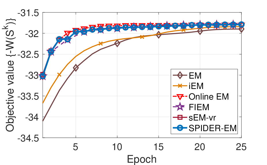
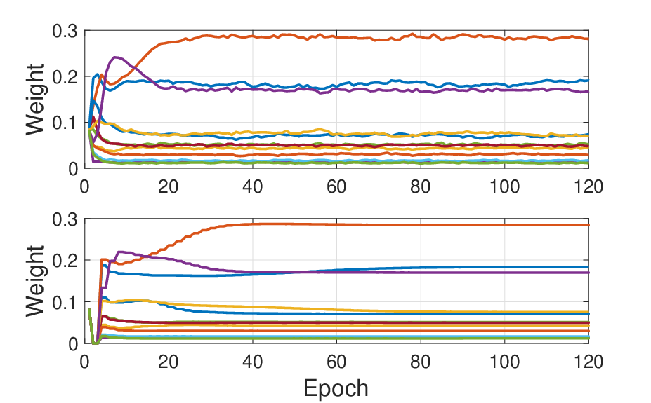
Figure 2: [Left] Evolution of the estimates of the weights αℓ\alpha_{\ell} for ℓ=1,…,g\ell=1,\ldots,g by Online EM (top) and SPIDER-EM (bottom) vs the number of epochs. [Right] Evolution of the objective function −W⁡(S^k)-\operatorname{W}(\widehat{S}_{k}) vs the number of epochs.

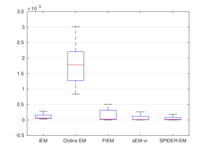
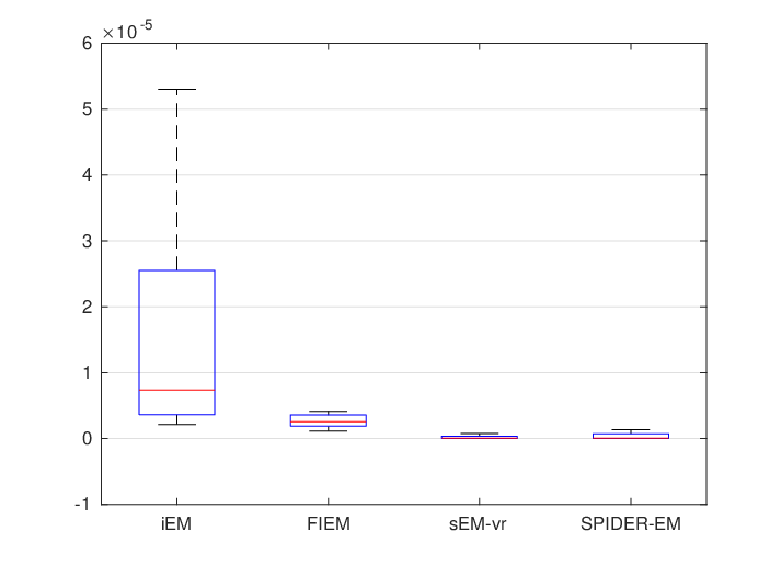
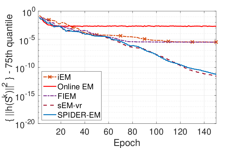
In Figure 2, we display the sequence of parameter estimates {θτ}\{\theta_{\tau}\}, the objective function {−W⁡(S^τ)}\{-\operatorname{W}(\widehat{S}_{\tau})\} and the squared norm of the mean field {‖h⁡(S^τ)‖2}\{\|h(\widehat{S}_{\tau})\|^{2}\}. Figure 3 gives insights on the distribution of ‖h⁡(S^t,k)‖2\|h(\widehat{S}_{t,k})\|^{2} along SPIDER-EM paths. The mini-batches {ℬτ}τ\{\mathcal{B}_{\tau}\}_{\tau} are independent, and sampled at random in {1,…,n}\{1,\ldots,n\} with replacement. For a fair comparison, we use the same seed to sample the minibatches {ℬk}\{\mathcal{B}_{k}\}; another seed is used for FIEM which requires a second sequence of minibatches {ℬ¯τ}τ\{\overline{\mathcal{B}}_{\tau}\}_{\tau}. The minibatch size is set to be 𝖻=100\mathsf{b}=100 and the stepsize γτ=5×10⁻³\gamma_{\tau}=5\times 10^{-3} except for iEM where γτ=1\gamma_{\tau}=1. The same initial value S^init\widehat{S}_{\mathrm{init}} is used for all experiments. We have implemented the procedure of [19] in order to obtain the initialization θinit\theta_{\mathrm{init}} and then we set S^init=defs¯​(θinit)\widehat{S}_{\mathrm{init}}\stackrel{{\scriptstyle\mathrm{def}}}{{=}}\bar{s}(\theta_{\mathrm{init}}) ( −W⁡(S^init)=−58.3-\operatorname{W}(\widehat{S}_{\mathrm{init}})=-58.3). The plots illustrate that SPIDER-EM reduces the variability of Online EM and compares favorably to iEM and FIEM. Additional details and results are given in the Supplementary material.

Refer to caption
Refer to caption
Figure 3: [Left] Quantile 0.250.25 and [Right] quantile 0.750.75 of the distribution of ‖h⁡(S^t,−1)‖2\|h(\widehat{S}_{t,-1})\|^{2} vs the number of epochs tt; the quantiles are estimated from 4040 independent samples of this distribution.

5 Conclusions

We have introduced the SPIDER-EM algorithm for large-scale inference. The algorithm offers low memory footprint and improved complexity bounds compared to the state-of-the-art, which is verified by theoretical analysis and numerical experiments.

Broader Impact

This work does not present any foreseeable societal consequence.

Acknowledgments and Disclosure of Funding

The work of G. Fort is partially supported by the Fondation Simone et Cino del Duca under the project OpSiMorE. The work of E. Moulines is partially supported by ANR-19-CHIA-0002-01 / chaire SCAI. It was partially prepared within the framework of the HSE University Basic Research Program. The work of H.-T. Wai is partially supported by the CUHK Direct Grant #4055113.

References

  • Balakrishnan et al. [2017] S. Balakrishnan, M. J. Wainwright, and B. Yu. Statistical guarantees for the EM algorithm: From population to sample-based analysis. Ann. Statist., 45(1):77–120, 2017.
  • Benveniste et al. [1990] A. Benveniste, M. Métivier, and P. Priouret. Adaptive Algorithms and Stochastic Approximations. Springer Verlag, 1990.
  • Borkar [2008] V. S. Borkar. Stochastic approximation. Cambridge University Press, Cambridge; Hindustan Book Agency, New Delhi, 2008. A dynamical systems viewpoint.
  • Bottou and Le Cun [2004] L. Bottou and Y. Le Cun. Large scale online learning. In S. Thrun, L. K. Saul, and B. Schölkopf, editors, Advances in Neural Information Processing Systems 16, pages 217–224. MIT Press, 2004.
  • Bühlmann et al. [2016] P. Bühlmann, P. Drineas, M. Kane, and M. van der Laan. Handbook of Big Data. Chapman & Hall/CRC Handbooks of Modern Statistical Methods. CRC Press, 2016. ISBN 9781482249088.
  • Cappé and Moulines [2009] O. Cappé and E. Moulines. On-line expectation-maximization algorithm for latent data models. J. R. Stat. Soc. Ser. B Stat. Methodol., 71(3):593–613, 2009.
  • Chen et al. [2018] J. Chen, J. Zhu, Y. Teh, and T. Zhang. Stochastic expectation maximization with variance reduction. In S. Bengio, H. Wallach, H. Larochelle, K. Grauman, N. Cesa-Bianchi, and R. Garnett, editors, Advances in Neural Information Processing Systems 31, pages 7967–7977. 2018.
  • Defazio et al. [2014] A. Defazio, F. Bach, and S. Lacoste-Julien. Saga: A fast incremental gradient method with support for non-strongly convex composite objectives. In Z. Ghahramani, M. Welling, C. Cortes, N. D. Lawrence, and K. Q. Weinberger, editors, Advances in Neural Information Processing Systems 27, pages 1646–1654. Curran Associates, Inc., 2014.
  • Delyon et al. [1999] B. Delyon, M. Lavielle, and E. Moulines. Convergence of a stochastic approximation version of the EM algorithm. Ann. Statist., 27(1):94–128, 1999. ISSN 0090-5364. doi: 10.1214/aos/1018031103. URL https://doi.org/10.1214/aos/1018031103.
  • Dempster et al. [1977] A. Dempster, N. Laird, and D. Rubin. Maximum Likelihood from Incomplete Data via the EM Algorithm. J. Roy. Stat. Soc. B Met., 39(1):1–38, 1977.
  • Fang et al. [2018] C. Fang, C. Li, Z. Lin, and T. Zhang. SPIDER: Near-Optimal Non-Convex Optimization via Stochastic Path-Integrated Differential Estimator. In S. Bengio, H. Wallach, H. Larochelle, K. Grauman, N. Cesa-Bianchi, and R. Garnett, editors, Advances in Neural Information Processing Systems 31, pages 689–699. Curran Associates, Inc., 2018.
  • Fort et al. [2020] G. Fort, P. Gach, and E. Moulines. Fast Incremental Expectation Maximization for non-convex optimization: non asymptotic convergence bounds. Technical report, HAL-02617725v1, 2020.
  • Ghadimi and Lan [2013] S. Ghadimi and G. Lan. Stochastic First- and Zeroth-Order Methods for Nonconvex Stochastic Programming. SIAM J. Optimiz., 23(4):2341–2368, 2013.
  • Härdle et al. [2018] W. Härdle, H. H.-S. Lu, and X. Shen. Handbook of big data analytics. Springer, 2018.
  • Johnson and Zhang [2013] R. Johnson and T. Zhang. Accelerating Stochastic Gradient Descent using Predictive Variance Reduction. In C. J. C. Burges, L. Bottou, M. Welling, Z. Ghahramani, and K. Q. Weinberger, editors, Advances in Neural Information Processing Systems 26, pages 315–323. Curran Associates, Inc., 2013.
  • Karimi et al. [2019a] B. Karimi, M. Lavielle, and E. Moulines. On the Convergence Properties of the Mini-Batch EM and MCEM Algorithms. Technical report, hal-02334485, 2019a.
  • Karimi et al. [2019b] B. Karimi, B. Miasojedow, E. Moulines, and H.-T. Wai. Non-asymptotic Analysis of Biased Stochastic Approximation Scheme. In COLT, 2019b.
  • Karimi et al. [2019c] B. Karimi, H.-T. Wai, E. Moulines, and M. Lavielle. On the Global Convergence of (Fast) Incremental Expectation Maximization Methods. In H. Wallach, H. Larochelle, A. Beygelzimer, F. d’Alché Buc, E. Fox, and R. Garnett, editors, Advances in Neural Information Processing Systems 32, pages 2837–2847. Curran Associates, Inc., 2019c.
  • Kwedlo [2015] W. Kwedlo. A new random approach for initialization of the multiple restart EM algorithm for Gaussian model-based clustering. Pattern Anal. Applic., 18:757–770, 2015.
  • McLachlan and Krishnan [2008] G. McLachlan and T. Krishnan. The EM algorithm and extensions. Wiley series in probability and statistics. Wiley, 2008.
  • Neal and Hinton [1998] R. M. Neal and G. E. Hinton. A View of the EM Algorithm that Justifies Incremental, Sparse, and other Variants. In M. I. Jordan, editor, Learning in Graphical Models, pages 355–368. Springer Netherlands, Dordrecht, 1998.
  • Ng and McLachlan [2003] S. K. Ng and G. J. McLachlan. On the choice of the number of blocks with the incremental EM algorithm for the fitting of normal mixtures. Stat. Comput., 13(1):45–55, 2003.
  • Nguyen et al. [2020] H. Nguyen, F. Forbes, and G. McLachlan. Mini-batch learning of exponential family finite mixture models. Stat. Comput., 2020.
  • Nguyen et al. [2017] L. M. Nguyen, J. Liu, K. Scheinberg, and M. Takáč. Sarah: A novel method for machine learning problems using stochastic recursive gradient. In Proceedings of the 34th International Conference on Machine Learning - Volume 70, ICML’17, page 2613–2621. JMLR.org, 2017.
  • Reddi et al. [2016] S. Reddi, S. Sra, B. Póczos, and A. Smola. Fast Incremental Method for Smooth Nonconvex Optimization. In 2016 IEEE 55th Conference on Decision and Control (CDC), pages 1971–1977, 2016.
  • Robbins and Monro [1951] H. Robbins and S. Monro. A stochastic approximation method. The annals of mathematical statistics, pages 400–407, 1951.
  • Wang et al. [2019] Z. Wang, K. Ji, Y. Zhou, Y. Liang, and V. Tarokh. SpiderBoost and Momentum: Faster Stochastic Variance Reduction Algorithms. In H. Wallach, H. Larochelle, A. Beygelzimer, F. d’ Alché-Buc, E. Fox, and R. Garnett, editors, Advances in Neural Information Processing Systems 32, pages 2406–2416. 2019.

Supplementary materials for “A Stochastic Path-Integrated Differential EstimatoR Expectation Maximization Algorithm”

Gersende Fort
Institut de Mathématiques de Toulouse
Université de Toulouse; CNRS
UPS, F-31062 Toulouse Cedex 9, France
gersende.fort@math.univ-toulouse.fr
&Eric Moulines
Centre de Mathématiques Appliquées
Ecole Polytechnique, France
CS Departement
HSE University, Russian Federation
eric.moulines@polytechnique.edu
&Hoi-To Wai
Department of SEEM
The Chinese University of Hong Kong
Shatin, Hong Kong
htwai@cuhk.edu.hk

Notations. For two vectors a,b∈ℝra,b\in\mathbb{R}^{r}, ⟨a,b⟩\left\langle a,b\right\rangle denotes the usual Euclidean product and ‖a‖\|a\| the associated norm. By convention, vectors are column vectors. For a vector xx with components (x1,…,xr)(x_{1},\ldots,x_{r}), xi:jx_{i:j} denotes the sub-vector with components (xi,xi+1,…,xj−1,xj)(x_{i},x_{i+1},\ldots,x_{j-1},x_{j}).

For two matrices A∈ℝr1×r2A\in\mathbb{R}^{r_{1}\times r_{2}} and B∈ℝr3×r4B\in\mathbb{R}^{r_{3}\times r_{4}}, A⊗BA\otimes B denotes the Kronecker product. Ir\mathrm{I}_{r} is the r×rr\times r identity matrix. ATA^{T} is the transpose of AA.

6 Complexity of incremental EM-based methods for smooth non-convex finite sum optimization

We first compare the complexities of the incremental EM based methods using the following table which summarizes the state-of-the-art results.

algorithm γ\gamma KOptK_{\operatorname{Opt}} KCEK_{\operatorname{CE}} Optimal KCEK_{\operatorname{CE}}
EM [10] - 1+kmax1+k_{\mathrm{max}} n+n​kmaxn+nk_{\mathrm{max}} N/A
online-EM [6] decaying; 𝒪(L−1k−1/2){\cal O}(L^{-1}k^{-1/2}) 1+kmax1+k_{\mathrm{max}} n+𝖻​kmaxn+\mathsf{b}k_{\mathrm{max}} ϵ−2\epsilon^{-2}
iEM [21] 1 1+kmax1+k_{\mathrm{max}} n+𝖻​kmaxn+\mathsf{b}k_{\mathrm{max}} ϵ−1​n\epsilon^{-1}n
sEM-vr [7, 18] O(L−1n−2/3)O(L^{-1}n^{-2/3}) 1+kin​kout1+k_{\mathrm{in}}k_{\mathrm{out}} n⁡(1+kout)+(𝖻​kin+n)​koutn(1+k_{\mathrm{out}})+(\mathsf{b}k_{\mathrm{in}}+n)k_{\mathrm{out}} ϵ−1​n2/3\epsilon^{-1}n^{2/3}
FIEM [18] O(L−1n−2/3)O(L^{-1}n^{-2/3}) 1+kmax1+k_{\mathrm{max}} n+2​𝖻​kmaxn+2\mathsf{b}k_{\mathrm{max}} ϵ−1​n2/3\epsilon^{-1}n^{2/3}
FIEM [12] O(L−1n−1/3kmax−1/3)O(L^{-1}n^{-1/3}k_{\mathrm{max}}^{-1/3}) 1+kmax1+k_{\mathrm{max}} n+2​𝖻​kmaxn+2\mathsf{b}k_{\mathrm{max}} ϵ−3/2n\epsilon^{-3/2}\sqrt{n}
SPIDER-EM O⁡(L−1)O(L^{-1}) 1+kin​kout1+k_{\mathrm{in}}k_{\mathrm{out}} n+kout​n+2​𝖻​kin​koutn+k_{\mathrm{out}}n+2\mathsf{b}k_{\mathrm{in}}k_{\mathrm{out}} ϵ−1​n\epsilon^{-1}\sqrt{n}
Table 1: Comparison between different EM-based algorithms for smooth non convex finite sum optimization. Except sEM-vr and SPIDER-EM which have nested loops (koutk_{\mathrm{out}} is the maximal number of outer loops and kink_{\mathrm{in}} is the number of inner loops per outer loop), kmaxk_{\mathrm{max}} is the maximal number of iterations. The last column is the optimal complexity to reach an ϵ\epsilon-approximate stationary point.

Next, we provide the psuedo-codes of several existing incremental EM-based algorithms, following the notations defined in the main paper.

Data: kmax∈ℕ⋆k_{\mathrm{max}}\in{\mathbb{N}}_{\star}, S^init∈ℝq\widehat{S}_{\mathrm{init}}\in{\mathbb{R}^{q}}
Result: The EM sequence: S^k,k=0,…,kmax\widehat{S}_{k},k=0,\ldots,k_{\mathrm{max}}
S^0=s¯∘𝖳⁡(S^init)\widehat{S}_{0}=\bar{s}\circ\mathsf{T}(\widehat{S}_{\mathrm{init}}) ; 1
for k=0,…,kmax−1k=0,\ldots,k_{\mathrm{max}}-1 do 2
S^k+1=s¯∘𝖳⁡(S^k)\widehat{S}_{k+1}=\bar{s}\circ\mathsf{T}(\widehat{S}_{k})
Algorithm 2 The EM algorithm in the expectation space.
Data: kmax∈ℕ⋆k_{\mathrm{max}}\in{\mathbb{N}}_{\star}, S^init∈ℝq\widehat{S}_{\mathrm{init}}\in{\mathbb{R}^{q}}, γk∈(0,∞)\gamma_{k}\in\left(0,\infty\right) for k=1,…,kmaxk=1,\ldots,k_{\mathrm{max}}
Result: The SA sequence: S^k,k=0,…,kmax\widehat{S}_{k},k=0,\ldots,k_{\mathrm{max}}
S^0=s¯∘𝖳⁡(S^init)\widehat{S}_{0}=\bar{s}\circ\mathsf{T}(\widehat{S}_{\mathrm{init}}) ; 1
for k=0,…,kmax−1k=0,\ldots,k_{\mathrm{max}}-1 do 2
Sample a mini-batch ℬk+1\mathcal{B}_{k+1} in {1,…,n}\{1,\ldots,n\} of size 𝖻\mathsf{b}, with replacement ; 3
    S^k+1=S^k+γk+1​(s¯ℬk+1∘𝖳⁡(S^k)−S^k)\widehat{S}_{k+1}=\widehat{S}_{k}+\gamma_{k+1}\left(\bar{s}_{\mathcal{B}_{k+1}}\circ\mathsf{T}(\widehat{S}_{k})-\widehat{S}_{k}\right).
Algorithm 3 The Online EM algorithm.
Data: kmax∈ℕ⋆k_{\mathrm{max}}\in{\mathbb{N}}_{\star}, S^init∈ℝq\widehat{S}_{\mathrm{init}}\in{\mathbb{R}^{q}}, γk∈(0,∞)\gamma_{k}\in\left(0,\infty\right) for k=1,…,kmaxk=1,\ldots,k_{\mathrm{max}}
Result: The iEM sequence: S^k,k=0,…,kmax\widehat{S}_{k},k=0,\ldots,k_{\mathrm{max}}
𝖲0,i=s¯i∘𝖳⁡(S^init)\mathsf{S}_{0,i}=\bar{s}_{i}\circ\mathsf{T}(\widehat{S}_{\mathrm{init}}) for all i=1,…,ni=1,\ldots,n; 1
S^0=S~0=n−1​∑i=1n𝖲0,i\widehat{S}_{0}=\widetilde{S}_{0}=n^{-1}\sum_{i=1}^{n}\mathsf{S}_{0,i}; 2
for k=0,…,kmax−1k=0,\ldots,k_{\mathrm{max}}-1 do 3
Sample a mini-batch ℬk+1\mathcal{B}_{k+1} in {1,…,n}\{1,\ldots,n\} of size 𝖻\mathsf{b}, with replacement ; 4
    𝖲k+1,i=𝖲k,i\mathsf{S}_{k+1,i}=\mathsf{S}_{k,i} for i∉ℬk+1i\notin\mathcal{B}_{k+1} ; 5
    𝖲k+1,i=s¯i∘𝖳⁡(S^k)\mathsf{S}_{k+1,i}=\bar{s}_{i}\circ\mathsf{T}(\widehat{S}_{k}) for i∈ℬk+1i\in\mathcal{B}_{k+1}; 6
    S~k+1=S~k+n−1​∑i∈ℬk+1(𝖲k+1,i−𝖲k,i)\widetilde{S}_{k+1}=\widetilde{S}_{k}+n^{-1}\sum_{i\in\mathcal{B}_{k+1}}\left(\mathsf{S}_{k+1,i}-\mathsf{S}_{k,i}\right) ; 7
    S^k+1=S^k+γk+1​(S~k+1−S^k)\widehat{S}_{k+1}=\widehat{S}_{k}+\gamma_{k+1}(\widetilde{S}_{k+1}-\widehat{S}^{k})
Algorithm 4 The Incremental EM (iEM) algorithm.
Data: kmax∈ℕ⋆k_{\mathrm{max}}\in{\mathbb{N}}_{\star}, S^init∈ℝq\widehat{S}_{\mathrm{init}}\in{\mathbb{R}^{q}}, γk∈(0,∞)\gamma_{k}\in\left(0,\infty\right) for k=1,…,kmaxk=1,\ldots,k_{\mathrm{max}}
Result: The FIEM sequence: S^k,k=0,…,kmax\widehat{S}_{k},k=0,\ldots,k_{\mathrm{max}}
𝖲0,i=s¯i∘𝖳⁡(S^init)\mathsf{S}_{0,i}=\bar{s}_{i}\circ\mathsf{T}(\widehat{S}_{\mathrm{init}}) for all i=1,…,ni=1,\ldots,n; 1
S^0=S~0=n−1​∑i=1n𝖲0,i\widehat{S}_{0}=\widetilde{S}_{0}=n^{-1}\sum_{i=1}^{n}\mathsf{S}_{0,i}; 2
for k=0,…,kmax−1k=0,\ldots,k_{\mathrm{max}}-1 do 3
Sample a mini-batch ℬk+1\mathcal{B}_{k+1} in {1,…,n}\{1,\ldots,n\} of size 𝖻\mathsf{b}, with replacement ; 4
    𝖲k+1,i=𝖲k,i\mathsf{S}_{k+1,i}=\mathsf{S}_{k,i} for i∉ℬk+1i\notin\mathcal{B}_{k+1} ; 5
    𝖲k+1,i=s¯i∘𝖳⁡(S^k)\mathsf{S}_{k+1,i}=\bar{s}_{i}\circ\mathsf{T}(\widehat{S}_{k}) for i∈ℬk+1i\in\mathcal{B}_{k+1} ; 6
    S~k+1=S~k+n−1​∑i∈ℬk+1(𝖲k+1,i−𝖲k,i)\widetilde{S}_{k+1}=\widetilde{S}_{k}+n^{-1}\sum_{i\in\mathcal{B}_{k+1}}\left(\mathsf{S}_{k+1,i}-\mathsf{S}_{k,i}\right) ; 7
    Sample a mini-batch ℬk+1′\mathcal{B}_{k+1}^{\prime} in {1,…,n}\{1,\ldots,n\} of size 𝖻\mathsf{b}, with replacement ; 8
    Vk+1=S~k+1−𝖻−1​∑i∈ℬk+1′𝖲k+1,iV_{k+1}=\widetilde{S}_{k+1}-\mathsf{b}^{-1}\sum_{i\in\mathcal{B}^{\prime}_{k+1}}\mathsf{S}_{k+1,i} ; 9
    S^k+1=S^k+γk+1​(s¯ℬk+1′∘𝖳⁡(S^k)−S^k+Vk+1)\widehat{S}_{k+1}=\widehat{S}_{k}+\gamma_{k+1}(\bar{s}_{\mathcal{B}^{\prime}_{k+1}}\circ\mathsf{T}(\widehat{S}_{k})-\widehat{S}_{k}+V_{k+1})
Algorithm 5 The Fast Incremental EM (FIEM) algorithm.
Data: kin∈ℕ⋆k_{\mathrm{in}}\in{\mathbb{N}}_{\star}, kout∈ℕ⋆k_{\mathrm{out}}\in{\mathbb{N}}_{\star}, S^init∈ℝq\widehat{S}_{\mathrm{init}}\in{\mathbb{R}^{q}}, γt,k∈(0,∞)\gamma_{t,k}\in\left(0,\infty\right) for t≥1,k≥1t\geq 1,k\geq 1
Result: The sEM-vr sequence: S^t,k,t=1,…,kout\widehat{S}_{t,k},t=1,\dots,k_{\mathrm{out}} and k=0,…,kin−1k=0,\ldots,k_{\mathrm{in}}-1
𝖲1,0=s¯∘𝖳⁡(S^init)\mathsf{S}_{1,0}=\bar{s}\circ\mathsf{T}(\widehat{S}_{\mathrm{init}}) ; 1
S^1,0=S^init\widehat{S}_{1,0}=\widehat{S}_{\mathrm{init}} ; 2
for t=1,…,koutt=1,\ldots,k_{\mathrm{out}} do 3
for k=0,…,kin−2k=0,\ldots,k_{\mathrm{in}}-2 do 4
   Sample a mini-batch ℬt,k+1\mathcal{B}_{t,k+1} in {1,…,n}\{1,\ldots,n\} of size 𝖻\mathsf{b}, with replacement ; 5
       Vt,k+1=𝖲t,0−s¯ℬt,k+1∘𝖳⁡(S^t−1,kin−1)V_{t,k+1}=\mathsf{S}_{t,0}-\bar{s}_{\mathcal{B}_{t,k+1}}\circ\mathsf{T}(\widehat{S}_{t-1,k_{\mathrm{in}}-1}) ; 6
       S^t,k+1=S^t,k+γt,k+1​(s¯ℬt,k+1∘𝖳⁡(S^t,k)−S^t,k+Vt,k+1)\widehat{S}_{t,k+1}=\widehat{S}_{t,k}+\gamma_{t,k+1}\left(\bar{s}_{\mathcal{B}_{t,k+1}}\circ\mathsf{T}(\widehat{S}_{t,k})-\widehat{S}_{t,k}+V_{t,k+1}\right)𝖲t+1,0=s¯∘𝖳⁡(S^t,kin−1)\mathsf{S}_{t+1,0}=\bar{s}\circ\mathsf{T}(\widehat{S}_{t,k_{\mathrm{in}}-1}) ; 7
    S^t+1,0=S^t,kin−1+γt,kin​(𝖲t+1,0−S^t,kin−1)\widehat{S}_{t+1,0}=\widehat{S}_{t,k_{\mathrm{in}}-1}+\gamma_{t,k_{\mathrm{in}}}\left(\mathsf{S}_{t+1,0}-\widehat{S}_{t,k_{\mathrm{in}}-1}\right)
Algorithm 6 The sEM-vr algorithm.

7 An equivalent definition of the SPIDER-EM algorithm

Using Lemma 7 below this page, we deduce that SPIDER-EM can be equivalently described by the following algorithm 7.

Data: kin∈ℕ⋆k_{\mathrm{in}}\in{\mathbb{N}}_{\star}, kout∈ℕ⋆k_{\mathrm{out}}\in{\mathbb{N}}_{\star}, S^init∈ℝq\widehat{S}_{\mathrm{init}}\in\mathbb{R}^{q}, a positive sequence {γt,k,t,k≥1}\{\gamma_{t,k},t,k\geq 1\}.
Result: The SPIDER-EM sequence: S^t,k\widehat{S}_{t,k}, t=1,…,koutt=1,\dots,k_{\mathrm{out}}, k=0,…,kin−1k=0,\dots,k_{\mathrm{in}}-1
S^1,−1=S^init\widehat{S}_{1,-1}=\widehat{S}_{\mathrm{init}} ; 1
S~1,0=s¯∘𝖳⁡(S^init)\widetilde{S}_{1,0}=\bar{s}\circ\mathsf{T}(\widehat{S}_{\mathrm{init}}) ; 2
for t=1,…,koutt=1,\ldots,k_{\mathrm{out}} do 3
Vt,0=0V_{t,0}=0 ; 4
    for k=0,…,kin−2k=0,\ldots,k_{\mathrm{in}}-2 do 5
   Sample a mini-batch ℬt,k+1\mathcal{B}_{t,k+1} in {1,…,n}\{1,\ldots,n\} of size 𝖻\mathsf{b}, with or without replacement ; 6
       Vt,k+1=Vt,k+S~t,k−s¯ℬt,k+1∘𝖳⁡(S^t,k−1)V_{t,k+1}=V_{t,k}+\widetilde{S}_{t,k}-\bar{s}_{\mathcal{B}_{t,k+1}}\circ\mathsf{T}(\widehat{S}_{t,k-1}) ; 7
       S~t,k+1=s¯ℬt,k+1∘𝖳⁡(S^t,k)\widetilde{S}_{t,k+1}=\bar{s}_{\mathcal{B}_{t,k+1}}\circ\mathsf{T}(\widehat{S}_{t,k}) ; 8
       S^t,k+1=S^t,k+γt,k+1​(S~t,k+1−S^t,k+Vt,k+1)\widehat{S}_{t,k+1}=\widehat{S}_{t,k}+\gamma_{t,k+1}\left(\widetilde{S}_{t,k+1}-\widehat{S}_{t,k}+V_{t,k+1}\right) S~t+1,0=s¯∘𝖳⁡(S^t,kin−1)\widetilde{S}_{t+1,0}=\bar{s}\circ\mathsf{T}(\widehat{S}_{t,k_{\mathrm{in}}-1}) ; 9
    S^t+1,0=S^t,kin−1+γt,kin​(S~t+1,0−S^t,kin−1)\widehat{S}_{t+1,0}=\widehat{S}_{t,k_{\mathrm{in}}-1}+\gamma_{t,k_{\mathrm{in}}}\left(\widetilde{S}_{t+1,0}-\widehat{S}_{t,k_{\mathrm{in}}-1}\right)
Algorithm 7 The SPIDER-EM algorithm (equivalent description)
Lemma 3.

Let {γk,k≥1}\{\gamma_{k},k\geq 1\} be a positive deterministic sequence and {ℬk,t,k≥1}\{\mathcal{B}_{k},t,k\geq 1\} be a family of mini-batches sampled from {1,…,n}\{1,\ldots,n\}. Fix S^−1,S^0\widehat{S}_{-1},\widehat{S}_{0} and 𝖲0\mathsf{S}_{0}. Define for k=0,⋯,kin−2k=0,\cdots,k_{\mathrm{in}}-2

{𝖲k+1=def𝖲k+s¯ℬk+1∘𝖳⁡(S^k)−s¯ℬk+1∘𝖳⁡(S^k−1),S^k+1=defS^k+γk+1​(𝖲k+1−S^k).\displaystyle\left\{\begin{array}[]{l}\mathsf{S}_{k+1}\stackrel{{\scriptstyle\mathrm{def}}}{{=}}\mathsf{S}_{k}+\bar{s}_{\mathcal{B}_{k+1}}\circ\mathsf{T}(\widehat{S}_{k})-\bar{s}_{\mathcal{B}_{k+1}}\circ\mathsf{T}(\widehat{S}_{k-1})\;,\\ \widehat{S}_{k+1}\stackrel{{\scriptstyle\mathrm{def}}}{{=}}\widehat{S}_{k}+\gamma_{k+1}\left(\mathsf{S}_{k+1}-\widehat{S}_{k}\right)\;.\end{array}\right.

Set S~−1=defS^−1\widetilde{S}_{-1}\stackrel{{\scriptstyle\mathrm{def}}}{{=}}\widehat{S}_{-1}, S~0=defS^0\widetilde{S}_{0}\stackrel{{\scriptstyle\mathrm{def}}}{{=}}\widehat{S}_{0}, V0=def0V_{0}\stackrel{{\scriptstyle\mathrm{def}}}{{=}}0 and define for k=0,…,kin−2k=0,\ldots,k_{\mathrm{in}}-2,

{Vk+1=defVk+s¯ℬk∘𝖳⁡(S~k−1)−s¯ℬk+1∘𝖳⁡(S~k−1),S~k+1=defS~k+γk+1​(s¯ℬk+1∘𝖳⁡(S~k)−S~k+Vk+1);\displaystyle\left\{\begin{array}[]{l}V_{k+1}\stackrel{{\scriptstyle\mathrm{def}}}{{=}}V_{k}+\bar{s}_{\mathcal{B}_{k}}\circ\mathsf{T}(\widetilde{S}_{k-1})-\bar{s}_{\mathcal{B}_{k+1}}\circ\mathsf{T}(\widetilde{S}_{k-1})\;,\\ \widetilde{S}_{k+1}\stackrel{{\scriptstyle\mathrm{def}}}{{=}}\widetilde{S}_{k}+\gamma_{k+1}\left(\bar{s}_{\mathcal{B}_{k+1}}\circ\mathsf{T}(\widetilde{S}_{k})-\widetilde{S}_{k}+V_{k+1}\right)\;;\end{array}\right.

by convention, set s¯ℬ0∘𝖳⁡(S~−1)=𝖲0\bar{s}_{\mathcal{B}_{0}}\circ\mathsf{T}(\widetilde{S}_{-1})=\mathsf{S}_{0}.

Then for any k=−1,…,kin−1k=-1,\ldots,k_{\mathrm{in}}-1, S~k=S^k\widetilde{S}_{k}=\widehat{S}_{k}.

Proof.

We prove by induction that for any k≥1k\geq 1, Vk=𝖲k−s¯ℬk∘𝖳⁡(S^k−1)V_{k}=\mathsf{S}_{k}-\bar{s}_{\mathcal{B}_{k}}\circ\mathsf{T}(\widehat{S}_{k-1}) and S~k=S^k\widetilde{S}_{k}=\widehat{S}_{k}. We have by definition of V0V_{0}, s¯ℬ0∘𝖳⁡(S~−1)\bar{s}_{\mathcal{B}_{0}}\circ\mathsf{T}(\widetilde{S}_{-1}), S~−1\widetilde{S}_{-1} and 𝖲1\mathsf{S}_{1},

V1\displaystyle V_{1} =𝖲0−s¯ℬ1∘𝖳⁡(S~−1)=𝖲0−s¯ℬ1∘𝖳⁡(S^−1)=𝖲1−s¯ℬ1∘𝖳⁡(S^0).\displaystyle=\mathsf{S}_{0}-\bar{s}_{\mathcal{B}_{1}}\circ\mathsf{T}(\widetilde{S}_{-1})=\mathsf{S}_{0}-\bar{s}_{\mathcal{B}_{1}}\circ\mathsf{T}(\widehat{S}_{-1})=\mathsf{S}_{1}-\bar{s}_{\mathcal{B}_{1}}\circ\mathsf{T}(\widehat{S}_{0})\;.

In addition, by definition of S~0\widetilde{S}_{0}, S~1\widetilde{S}_{1} and V1V_{1}, we have

S~1\displaystyle\widetilde{S}_{1} =S^0+γ1​(s¯ℬ1∘𝖳⁡(S^0)−S^0+𝖲1−s¯ℬ1∘𝖳⁡(S^−0)).\displaystyle=\widehat{S}_{0}+\gamma_{1}\left(\bar{s}_{\mathcal{B}_{1}}\circ\mathsf{T}(\widehat{S}_{0})-\widehat{S}_{0}+\mathsf{S}_{1}-\bar{s}_{\mathcal{B}_{1}}\circ\mathsf{T}(\widehat{S}_{-0})\right)\;.

Assume that the property holds for any 0≤j≤k0\leq j\leq k. Then, by definition of Vk+1V_{k+1}, the induction assumption on VkV_{k} and the definition of 𝖲k+1\mathsf{S}_{k+1}, it holds

Vk+1\displaystyle V_{k+1} =Vk+s¯ℬk∘𝖳⁡(S~k−1)−s¯ℬk+1∘𝖳⁡(S~k−1)\displaystyle=V_{k}+\bar{s}_{\mathcal{B}_{k}}\circ\mathsf{T}(\widetilde{S}_{k-1})-\bar{s}_{\mathcal{B}_{k+1}}\circ\mathsf{T}(\widetilde{S}_{k-1})
=𝖲k−s¯ℬk+1∘𝖳⁡(S~k−1)=𝖲k+1−s¯ℬk+1∘𝖳⁡(S~k).\displaystyle=\mathsf{S}_{k}-\bar{s}_{\mathcal{B}_{k+1}}\circ\mathsf{T}(\widetilde{S}_{k-1})=\mathsf{S}_{k+1}-\bar{s}_{\mathcal{B}_{k+1}}\circ\mathsf{T}(\widetilde{S}_{k})\;.

This concludes the induction for the property on {Vk,k≥0}\{V_{k},k\geq 0\}. In addition, by the induction assumption on S~k\widetilde{S}_{k}, the definition of Vk+1V_{k+1}, the induction assumption on VkV_{k} and the definition of 𝖲k+1\mathsf{S}_{k+1}, we have

S~k+1\displaystyle\widetilde{S}_{k+1} =S^k+γk+1​(s¯ℬk+1∘𝖳⁡(S^k)−S^k+Vk+s¯ℬk∘𝖳⁡(S^k−1)−s¯ℬk+1∘𝖳⁡(S^k−1))\displaystyle=\widehat{S}_{k}+\gamma_{k+1}\left(\bar{s}_{\mathcal{B}_{k+1}}\circ\mathsf{T}(\widehat{S}_{k})-\widehat{S}_{k}+V_{k}+\bar{s}_{\mathcal{B}_{k}}\circ\mathsf{T}(\widehat{S}_{k-1})-\bar{s}_{\mathcal{B}_{k+1}}\circ\mathsf{T}(\widehat{S}_{k-1})\right)
=S^k+γk+1​(s¯ℬk+1∘𝖳⁡(S^k)−S^k+𝖲k−s¯ℬk+1∘𝖳⁡(S^k−1))\displaystyle=\widehat{S}_{k}+\gamma_{k+1}\left(\bar{s}_{\mathcal{B}_{k+1}}\circ\mathsf{T}(\widehat{S}_{k})-\widehat{S}_{k}+\mathsf{S}_{k}-\bar{s}_{\mathcal{B}_{k+1}}\circ\mathsf{T}(\widehat{S}_{k-1})\right)
=S^k+γk+1​(𝖲k+1−S^k)=S^k+1.\displaystyle=\widehat{S}_{k}+\gamma_{k+1}\left(\mathsf{S}_{k+1}-\widehat{S}_{k}\right)=\widehat{S}_{k+1}\;.

This concludes the proof. ∎

8 General convergence results

The purpose of this section is to show the general convergence results of a SPIDER-EM like algorithm, and these results will be specialized in section 9. For all i=1,…,ni=1,\ldots,n, s¯i∘𝖳\bar{s}_{i}\circ\mathsf{T} is a function from ℝq\mathbb{R}^{q} to ℝq\mathbb{R}^{q}; for a selection of 𝖻\mathsf{b} indices ℬ\mathcal{B} in {1,…,n}\{1,\ldots,n\} with or without replacement, we set s¯ℬ∘𝖳=def𝖻−1​∑i∈ℬs¯i∘𝖳\bar{s}_{\mathcal{B}}\circ\mathsf{T}\stackrel{{\scriptstyle\mathrm{def}}}{{=}}\mathsf{b}^{-1}\sum_{i\in\mathcal{B}}\bar{s}_{i}\circ\mathsf{T}. More generally, s¯∘𝖳=defn−1​∑i=1ns¯i∘𝖳\bar{s}\circ\mathsf{T}\stackrel{{\scriptstyle\mathrm{def}}}{{=}}n^{-1}\sum_{i=1}^{n}\bar{s}_{i}\circ\mathsf{T}. For some results below, specific assumptions may be introduced on s¯t∘𝖳\bar{s}_{t}\circ\mathsf{T}.

Let {γk,k≥1}\{\gamma_{k},k\geq 1\} be a positive deterministic sequence. Let {ℬk,k≥1}\{\mathcal{B}_{k},k\geq 1\} be a family of independent random mini batches sampled in {1,…,n}\{1,\ldots,n\} of size 𝖻\mathsf{b}, (either with replacement or without replacement). Finally, let U−1,U0U_{-1},U_{0} be random variables. Assume that (U−1,U0)(U_{-1},U_{0}) are independent from the sequences {ℬk,k≥1}\{\mathcal{B}_{k},k\geq 1\} and set

U~0=defs¯∘𝖳⁡(U−1)=𝔼⁡[s¯ℬ1∘𝖳⁡(U−1)|U−1].\widetilde{U}_{0}\stackrel{{\scriptstyle\mathrm{def}}}{{=}}\bar{s}\circ\mathsf{T}(U_{-1})=\mathbb{E}\left[\bar{s}_{\mathcal{B}_{1}}\circ\mathsf{T}(U_{-1})|U_{-1}\right]\;. (16)

Consider the recursive definition for k≥0k\geq 0,

U~k+1\displaystyle\widetilde{U}_{k+1} =U~k+s¯ℬk+1∘𝖳⁡(Uk)−s¯ℬk+1∘𝖳⁡(Uk−1),\displaystyle=\widetilde{U}_{k}+\bar{s}_{\mathcal{B}_{k+1}}\circ\mathsf{T}(U_{k})-\bar{s}_{\mathcal{B}_{k+1}}\circ\mathsf{T}(U_{k-1})\;,
Uk+1\displaystyle U_{k+1} =Uk+γk+1​(U~k+1−Uk).\displaystyle=U_{k}+\gamma_{k+1}\left(\widetilde{U}_{k+1}-U_{k}\right)\;.

Finally, define the filtration

𝒢0=defσ⁡(U−1,U0),for k≥0,𝒢k+1=defσ⁡(𝒢k∪ℬk+1),\mathcal{G}_{0}\stackrel{{\scriptstyle\mathrm{def}}}{{=}}\sigma(U_{-1},U_{0}),\qquad\qquad\text{for $k\geq 0$,}\ \ \mathcal{G}_{k+1}\stackrel{{\scriptstyle\mathrm{def}}}{{=}}\sigma\left(\mathcal{G}_{k}\cup\mathcal{B}_{k+1}\right)\;,

and define the sequence of random variables

Δ0=defh⁡(U−1),for k≥0,Δk+1=defU~k+1−Uk=γk+1−1​(Uk+1−Uk).\Delta_{0}\stackrel{{\scriptstyle\mathrm{def}}}{{=}}h(U_{-1}),\qquad\qquad\text{for $k\geq 0$,}\ \ \Delta_{k+1}\stackrel{{\scriptstyle\mathrm{def}}}{{=}}\widetilde{U}_{k+1}-U_{k}=\gamma_{k+1}^{-1}(U_{k+1}-U_{k})\;.
Lemma 4.

For any k≥0k\geq 0, ℬk+1\mathcal{B}_{k+1} and 𝒢k\mathcal{G}_{k} are independent. For any u∈ℝqu\in\mathbb{R}^{q},

𝔼⁡[s¯ℬk+1∘𝖳⁡(u)]=s¯∘𝖳⁡(u).\mathbb{E}\left[\bar{s}_{\mathcal{B}_{k+1}}\circ\mathsf{T}(u)\right]=\bar{s}\circ\mathsf{T}(u)\;.

Assume that s¯i∘𝖳\bar{s}_{i}\circ\mathsf{T} is globally Lipschitz with constant LiL_{i}; set L2=defn−1​∑i=1nLi2L^{2}\stackrel{{\scriptstyle\mathrm{def}}}{{=}}n^{-1}\sum_{i=1}^{n}L_{i}^{2}. For any u,u′∈ℝqu,u^{\prime}\in\mathbb{R}^{q},

𝔼⁡[‖s¯ℬk+1∘𝖳⁡(u)−s¯ℬk+1∘𝖳⁡(u′)−s¯∘𝖳⁡(u)+s¯∘𝖳⁡(u′)‖2]≤1𝖻​(L2​‖u−u′‖2−‖s¯∘𝖳⁡(u)−s¯∘𝖳⁡(u′)‖2).\mathbb{E}\left[\|\bar{s}_{\mathcal{B}_{k+1}}\circ\mathsf{T}(u)-\bar{s}_{\mathcal{B}_{k+1}}\circ\mathsf{T}(u^{\prime})-\bar{s}\circ\mathsf{T}(u)+\bar{s}\circ\mathsf{T}(u^{\prime})\|^{2}\right]\\ \leq\frac{1}{\mathsf{b}}\left(L^{2}\|u-u^{\prime}\|^{2}-\|\bar{s}\circ\mathsf{T}(u)-\bar{s}\circ\mathsf{T}(u^{\prime})\|^{2}\right)\;.
Proof.

By assumption, ℬk+1\mathcal{B}_{k+1} and (U0,U−1)(U_{0},U_{-1}) are independent, and therefore ℬk+1\mathcal{B}_{k+1} and 𝒢0\mathcal{G}_{0} are also. In addition, ℬk+1\mathcal{B}_{k+1} is independent of ℬℓ\mathcal{B}_{\ell} for any ℓ≤k\ell\leq k so ℬk+1\mathcal{B}_{k+1} is independent of 𝒢k\mathcal{G}_{k}.

∙\bullet Case: sampling with replacement. We write ℬk+1={I1,⋯,I𝖻}\mathcal{B}_{k+1}=\{I_{1},\cdots,I_{\mathsf{b}}\} where the random variables are independent, and uniformly distributed on {1,⋯,n}\{1,\cdots,n\}. Then

𝔼⁡[s¯ℬk+1∘𝖳⁡(u)]=1𝖻​∑ℓ=1𝖻𝔼⁡[s¯Iℓ∘𝖳⁡(u)]=𝔼⁡[s¯I1∘𝖳⁡(u)]=s¯∘𝖳⁡(u).\mathbb{E}\left[\bar{s}_{\mathcal{B}_{k+1}}\circ\mathsf{T}(u)\right]=\frac{1}{\mathsf{b}}\sum_{\ell=1}^{\mathsf{b}}\mathbb{E}\left[\bar{s}_{I_{\ell}}\circ\mathsf{T}(u)\right]=\mathbb{E}\left[\bar{s}_{I_{1}}\circ\mathsf{T}(u)\right]=\bar{s}\circ\mathsf{T}(u)\;.

In addition, since the variance of the sum is the sum of the variance for independent r.v.

𝔼⁡[‖s¯ℬk+1∘𝖳⁡(u)−s¯ℬk+1∘𝖳⁡(u′)−s¯∘𝖳⁡(u)+s¯∘𝖳⁡(u′)‖2]\displaystyle\mathbb{E}\left[\|\bar{s}_{\mathcal{B}_{k+1}}\circ\mathsf{T}(u)-\bar{s}_{\mathcal{B}_{k+1}}\circ\mathsf{T}(u^{\prime})-\bar{s}\circ\mathsf{T}(u)+\bar{s}\circ\mathsf{T}(u^{\prime})\|^{2}\right]
=1𝖻2​∑ℓ=1𝖻𝔼⁡[‖s¯Iℓ∘𝖳⁡(u)−s¯Iℓ∘𝖳⁡(u′)−s¯∘𝖳⁡(u)+s¯∘𝖳⁡(u′)‖2]\displaystyle\qquad=\frac{1}{\mathsf{b}^{2}}\sum_{\ell=1}^{\mathsf{b}}\mathbb{E}\left[\|\bar{s}_{I_{\ell}}\circ\mathsf{T}(u)-\bar{s}_{I_{\ell}}\circ\mathsf{T}(u^{\prime})-\bar{s}\circ\mathsf{T}(u)+\bar{s}\circ\mathsf{T}(u^{\prime})\|^{2}\right]

Then we have

𝔼⁡[‖s¯Iℓ∘𝖳⁡(u)−s¯Iℓ∘𝖳⁡(u′)−s¯∘𝖳⁡(u)+s¯∘𝖳⁡(u′)‖2]\displaystyle\mathbb{E}\left[\|\bar{s}_{I_{\ell}}\circ\mathsf{T}(u)-\bar{s}_{I_{\ell}}\circ\mathsf{T}(u^{\prime})-\bar{s}\circ\mathsf{T}(u)+\bar{s}\circ\mathsf{T}(u^{\prime})\|^{2}\right]
=1n​∑i=1n𝔼⁡[‖s¯i∘𝖳⁡(u)−s¯i∘𝖳⁡(u′)‖2]−‖s¯∘𝖳⁡(u)+s¯∘𝖳⁡(u′)‖2\displaystyle\qquad=\frac{1}{n}\sum_{i=1}^{n}\mathbb{E}\left[\|\bar{s}_{i}\circ\mathsf{T}(u)-\bar{s}_{i}\circ\mathsf{T}(u^{\prime})\|^{2}\right]-\|\bar{s}\circ\mathsf{T}(u)+\bar{s}\circ\mathsf{T}(u^{\prime})\|^{2}
≤‖u−u′‖2​1n​∑i=1nLi2−‖s¯∘𝖳⁡(u)+s¯∘𝖳⁡(u′)‖2\displaystyle\qquad\leq\|u-u^{\prime}\|^{2}\frac{1}{n}\sum_{i=1}^{n}L_{i}^{2}-\|\bar{s}\circ\mathsf{T}(u)+\bar{s}\circ\mathsf{T}(u^{\prime})\|^{2} (17)

which concludes the proof.

∙\bullet Case: sampling with no replacement. I1I_{1} is a uniform random variable on {1,⋯,n}\{1,\cdots,n\} so that 𝔼⁡[s¯I1∘𝖳⁡(u)]=s¯∘𝖳⁡(u)\mathbb{E}\left[\bar{s}_{I_{1}}\circ\mathsf{T}(u)\right]=\bar{s}\circ\mathsf{T}(u). Conditionally to I1I_{1}, I2I_{2} is a uniform random variable on {1,⋯,n}∖{I1}\{1,\cdots,n\}\setminus\{I_{1}\}. Therefore

𝔼⁡[s¯I2∘𝖳⁡(u)]=1n−1​(∑j=1ns¯j∘𝖳⁡(u)−𝔼⁡[s¯I1∘𝖳⁡(u)])=nn−1​s¯∘𝖳⁡(u)−1n−1​s¯∘𝖳⁡(u).\mathbb{E}\left[\bar{s}_{I_{2}}\circ\mathsf{T}(u)\right]=\ \frac{1}{n-1}\left(\sum_{j=1}^{n}\bar{s}_{j}\circ\mathsf{T}(u)-\mathbb{E}\left[\bar{s}_{I_{1}}\circ\mathsf{T}(u)\right]\right)=\frac{n}{n-1}\bar{s}\circ\mathsf{T}(u)-\frac{1}{n-1}\bar{s}\circ\mathsf{T}(u)\;.

By induction, for any ℓ≥2\ell\geq 2,

𝔼⁡[s¯Iℓ∘𝖳⁡(u)]\displaystyle\mathbb{E}\left[\bar{s}_{I_{\ell}}\circ\mathsf{T}(u)\right] =1n−ℓ+1​(∑j=1ns¯j∘𝖳⁡(u)−∑q=1ℓ−1𝔼⁡[s¯Iq∘𝖳⁡(u)])\displaystyle=\ \frac{1}{n-\ell+1}\left(\sum_{j=1}^{n}\bar{s}_{j}\circ\mathsf{T}(u)-\sum_{q=1}^{\ell-1}\mathbb{E}\left[\bar{s}_{I_{q}}\circ\mathsf{T}(u)\right]\right)
=nn−ℓ+1​s¯∘𝖳⁡(u)−ℓ−1n−ℓ+1​s¯∘𝖳⁡(u).\displaystyle=\frac{n}{n-\ell+1}\bar{s}\circ\mathsf{T}(u)-\frac{\ell-1}{n-\ell+1}\bar{s}\circ\mathsf{T}(u)\;.

As a conclusion, 𝖻−1​∑ℓ=1𝖻𝔼⁡[s¯Iℓ∘𝖳⁡(u)]=s¯∘𝖳⁡(u)\mathsf{b}^{-1}\,\sum_{\ell=1}^{\mathsf{b}}\mathbb{E}\left[\bar{s}_{I_{\ell}}\circ\mathsf{T}(u)\right]=\bar{s}\circ\mathsf{T}(u). Let u,u′∈ℝqu,u^{\prime}\in\mathbb{R}^{q}; set ϕ⁡(Iℓ)=defs¯Iℓ∘𝖳⁡(u)−s¯∘𝖳⁡(u)+s¯Iℓ∘𝖳⁡(u′)−s¯∘𝖳⁡(u′)\phi({I_{\ell}})\stackrel{{\scriptstyle\mathrm{def}}}{{=}}\bar{s}_{I_{\ell}}\circ\mathsf{T}(u)-\bar{s}\circ\mathsf{T}(u)+\bar{s}_{I_{\ell}}\circ\mathsf{T}(u^{\prime})-\bar{s}\circ\mathsf{T}(u^{\prime}). Then 𝔼⁡[ϕ⁡(Iℓ)]=0\mathbb{E}\left[\phi(I_{\ell})\right]=0. We first prove by induction that 𝔼⁡[‖ϕ⁡(Iℓ)‖2]=𝔼⁡[‖ϕ⁡(I1)‖2]\mathbb{E}\left[\|\phi(I_{\ell})\|^{2}\right]=\mathbb{E}\left[\|\phi(I_{1})\|^{2}\right]. Upon noting that I1I_{1} is a uniform random variable on {1,⋯,n}\{1,\cdots,n\},

𝔼⁡[‖ϕ⁡(Iℓ)‖2]\displaystyle\mathbb{E}\left[\|\phi(I_{\ell})\|^{2}\right] =1n−ℓ+1​(∑i=1n‖ϕ⁡(i)‖2−𝔼⁡[‖ϕ⁡(I1)‖2+⋯+‖ϕ⁡(Iℓ−1)‖2])\displaystyle=\frac{1}{n-\ell+1}\left(\sum_{i=1}^{n}\|\phi(i)\|^{2}-\mathbb{E}\left[\|\phi(I_{1})\|^{2}+\cdots+\|\phi(I_{\ell-1})\|^{2}\right]\right)
=nn−ℓ+1​𝔼​[‖ϕ⁡(I1)‖2]−1n−ℓ+1​∑p=1ℓ−1𝔼⁡[‖ϕ⁡(Ip)‖2]\displaystyle=\frac{n}{n-\ell+1}\mathbb{E}\left[\|\phi(I_{1})\|^{2}\right]-\frac{1}{n-\ell+1}\sum_{p=1}^{\ell-1}\mathbb{E}\left[\|\phi(I_{p})\|^{2}\right]

which concludes the induction. Second, let us prove that for any ℓ≥0\ell\geq 0,

𝔼⁡[‖∑p=1ℓ+1ϕ⁡(Ip)‖2]≤(ℓ+1)​𝔼​[‖ϕ⁡(I1)‖2].\mathbb{E}\left[\|\sum_{p=1}^{\ell+1}\phi(I_{p})\|^{2}\right]\leq(\ell+1)\mathbb{E}\left[\|\phi(I_{1})\|^{2}\right]\;. (18)

Since n−1​∑i=1nϕ⁡(i)=𝔼⁡[ϕ⁡(I1)]=0n^{-1}\sum_{i=1}^{n}\phi(i)=\mathbb{E}\left[\phi(I_{1})\right]=0,

𝔼⁡[⟨∑p=1ℓϕ⁡(Ip),ϕ⁡(Iℓ+1)⟩]=1n−ℓ​𝔼​[⟨∑p=1ℓϕ⁡(Ip),∑i=1nϕ⁡(i)−∑p=1ℓϕ⁡(Ip)⟩]=−1n−ℓ​𝔼​[‖∑p=1ℓϕ⁡(Ip)‖2],\mathbb{E}\left[\left\langle\sum_{p=1}^{\ell}\phi(I_{p}),\phi(I_{\ell+1})\right\rangle\right]=\frac{1}{n-\ell}\mathbb{E}\left[\left\langle\sum_{p=1}^{\ell}\phi(I_{p}),\sum_{i=1}^{n}\phi(i)-\sum_{p=1}^{\ell}\phi(I_{p})\right\rangle\right]=-\frac{1}{n-\ell}\mathbb{E}\left[\|\sum_{p=1}^{\ell}\phi(I_{p})\|^{2}\right]\;,

so that

𝔼⁡[‖∑p=1ℓ+1ϕ⁡(Ip)‖2]=(1−2n−ℓ)​𝔼​[‖∑p=1ℓϕ⁡(Ip)‖2]+𝔼⁡[‖ϕ⁡(Iℓ+1)‖2]≤(ℓ+1)​𝔼​[‖ϕ⁡(I1)‖2].\mathbb{E}\left[\|\sum_{p=1}^{\ell+1}\phi(I_{p})\|^{2}\right]=\left(1-\frac{2}{n-\ell}\right)\mathbb{E}\left[\|\sum_{p=1}^{\ell}\phi(I_{p})\|^{2}\right]+\mathbb{E}\left[\|\phi(I_{\ell+1})\|^{2}\right]\leq(\ell+1)\mathbb{E}\left[\|\phi(I_{1})\|^{2}\right]\;.

The proof follows from (18) and (17) since here again, I1I_{1} is uniformly distributed on {1,⋯,n}\{1,\cdots,n\}. ∎

Lemma 5.

For any k≥0k\geq 0,

𝔼⁡[Δk+1|𝒢k]−h⁡(Uk)=Δk−h⁡(Uk−1).\mathbb{E}\left[\Delta_{k+1}|\mathcal{G}_{k}\right]-h(U_{k})=\Delta_{k}-h(U_{k-1})\;.
Proof.

Let k≥0k\geq 0. Since conditionally to 𝒢k\mathcal{G}_{k}, ℬk+1={I1,…,I𝖻}\mathcal{B}_{k+1}=\{I_{1},\ldots,I_{\mathsf{b}}\} where the random variables IkI_{k}’s are independent and uniformly distributed on {1,…,n}\{1,\ldots,n\}, we have

𝔼⁡[U~k+1|𝒢k]=U~k+s¯∘𝖳⁡(Uk)−s¯∘𝖳⁡(Uk−1).\mathbb{E}\left[\widetilde{U}_{k+1}|\mathcal{G}_{k}\right]=\widetilde{U}_{k}+\bar{s}\circ\mathsf{T}(U_{k})-\bar{s}\circ\mathsf{T}(U_{k-1})\;.

In the case k=0k=0, we have by using (16)

𝔼⁡[Δ1−h⁡(U0)|𝒢0]=𝔼⁡[U~1|𝒢0]−s¯∘𝖳⁡(U0)=0=Δ0−h⁡(U−1);\mathbb{E}\left[\Delta_{1}-h(U_{0})|\mathcal{G}_{0}\right]=\mathbb{E}\left[\widetilde{U}_{1}|\mathcal{G}_{0}\right]-\bar{s}\circ\mathsf{T}(U_{0})=0=\Delta_{0}-h(U_{-1})\;;

the last equality explains the convention for Δ0\Delta_{0}. In the case k>0k>0,

𝔼⁡[Δk+1|𝒢k]\displaystyle\mathbb{E}\left[\Delta_{k+1}|\mathcal{G}_{k}\right] =𝔼⁡[U~k+1−Uk|𝒢k]=U~k+h⁡(Uk)−s¯∘𝖳⁡(Uk−1)\displaystyle=\mathbb{E}\left[\widetilde{U}_{k+1}-U_{k}|\mathcal{G}_{k}\right]=\widetilde{U}_{k}+h(U_{k})-\bar{s}\circ\mathsf{T}(U_{k-1})
=Δk+Uk−1+h⁡(Uk)−∘¯​𝖳​(Uk−1)=h⁡(Uk)+Δk−h⁡(Uk−1).\displaystyle=\Delta_{k}+U_{k-1}+h(U_{k})-\bar{\circ}\mathsf{T}(U_{k-1})=h(U_{k})+\Delta_{k}-h(U_{k-1})\;.

∎

Proposition 6.

Assume that for all i=1,⋯,ni=1,\cdots,n, s¯i∘𝖳\bar{s}_{i}\circ\mathsf{T} is globally Lipschitz, with constant LiL_{i}; set L2=defn−1​∑i=1nLi2L^{2}\stackrel{{\scriptstyle\mathrm{def}}}{{=}}n^{-1}\sum_{i=1}^{n}L_{i}^{2}. Then Δ0−𝔼⁡[Δ0|𝒢0]=0\Delta_{0}-\mathbb{E}\left[\Delta_{0}|\mathcal{G}_{0}\right]=0,

𝔼⁡[‖Δ1−𝔼⁡[Δ1|𝒢0]‖2|𝒢0]=𝔼⁡[‖Δ1−h⁡(U0)‖2|𝒢0]≤−1𝖻​‖s¯∘𝖳⁡(U0)−s¯∘𝖳⁡(U−1)‖2+L2𝖻​‖U0−U−1‖2.\mathbb{E}[\|\Delta_{1}-\mathbb{E}\left[\Delta_{1}|\mathcal{G}_{0}\right]\|^{2}|\mathcal{G}_{0}]=\mathbb{E}[\|\Delta_{1}-h(U_{0})\|^{2}|\mathcal{G}_{0}]\\ \leq-\frac{1}{\mathsf{b}}\|\bar{s}\circ\mathsf{T}(U_{0})-\bar{s}\circ\mathsf{T}(U_{-1})\|^{2}+\frac{L^{2}}{\mathsf{b}}\|U_{0}-U_{-1}\|^{2}\;.

and for any k≥1k\geq 1,

𝔼⁡[‖Δk+1−𝔼⁡[Δk+1|𝒢k]‖2|𝒢k]\displaystyle\mathbb{E}[\|\Delta_{k+1}-\mathbb{E}[\Delta_{k+1}|\mathcal{G}_{k}]\|^{2}|\mathcal{G}_{k}] ≤−1𝖻​‖s¯∘𝖳⁡(Uk)−s¯∘𝖳⁡(Uk−1)‖2+L2𝖻​γk2​‖Δk‖2;\displaystyle\leq-\frac{1}{\mathsf{b}}\|\bar{s}\circ\mathsf{T}(U_{k})-\bar{s}\circ\mathsf{T}(U_{k-1})\|^{2}+\frac{L^{2}}{\mathsf{b}}\gamma_{k}^{2}\,\|\Delta_{k}\|^{2}\;;
𝔼⁡[‖Δk+1−h⁡(Uk)‖2|𝒢0]\displaystyle\mathbb{E}[\|\Delta_{k+1}-h(U_{k})\|^{2}|\mathcal{G}_{0}] ≤−1𝖻∑j=0k𝔼[∥s¯∘𝖳(Uj)−s¯∘𝖳(Uj−1)∥2|𝒢0]\displaystyle\leq-\frac{1}{\mathsf{b}}\sum_{j=0}^{k}\mathbb{E}\left[\|\bar{s}\circ\mathsf{T}(U_{j})-\bar{s}\circ\mathsf{T}(U_{j-1})\|^{2}|\mathcal{G}_{0}\right]
+L2𝖻​(∑j=1kγj2​𝔼​[‖Δj‖2|𝒢0]+‖U0−U−1‖2).\displaystyle+\frac{L^{2}}{\mathsf{b}}\left(\sum_{j=1}^{k}\gamma_{j}^{2}\,\mathbb{E}\left[\|\Delta_{j}\|^{2}|\mathcal{G}_{0}\right]+\|U_{0}-U_{-1}\|^{2}\right)\;.
Proof.

The statement on Δ0\Delta_{0} is trivial since Δ0=h⁡(U−1)∈𝒢0\Delta_{0}=h(U_{-1})\in\mathcal{G}_{0}. By definition of Δ1\Delta_{1}, by Section 8 and by (16)

𝔼⁡[Δ1|𝒢0]=𝔼⁡[U~1|𝒢0]−U0=U~0+s¯∘𝖳⁡(U0)−s¯∘𝖳⁡(U−1)−U0=h⁡(U0).\mathbb{E}\left[\Delta_{1}|\mathcal{G}_{0}\right]=\mathbb{E}\left[\widetilde{U}_{1}|\mathcal{G}_{0}\right]-U_{0}=\widetilde{U}_{0}+\bar{s}\circ\mathsf{T}(U_{0})-\bar{s}\circ\mathsf{T}(U_{-1})-U_{0}=h(U_{0})\;.

The equation

Δ1−𝔼⁡[Δ1|𝒢0]=s¯ℬ1∘𝖳⁡(U0)−s¯ℬ1∘𝖳⁡(U−1)−(s¯∘𝖳⁡(U0)−s¯∘𝖳⁡(U−1))\Delta_{1}-\mathbb{E}\left[\Delta_{1}|\mathcal{G}_{0}\right]=\bar{s}_{\mathcal{B}_{1}}\circ\mathsf{T}(U_{0})-\bar{s}_{\mathcal{B}_{1}}\circ\mathsf{T}(U_{-1})-\left(\bar{s}\circ\mathsf{T}(U_{0})-\bar{s}\circ\mathsf{T}(U_{-1})\right)

and Section 8 provides the upper bound for Δ1\Delta_{1}. Let k≥1k\geq 1. By definition of Δk+1\Delta_{k+1} and by Section 8,

Δk+1−𝔼⁡[Δk+1|𝒢k]\displaystyle\Delta_{k+1}-\mathbb{E}\left[\Delta_{k+1}|\mathcal{G}_{k}\right] =U~k+1−𝔼⁡[U~k+1|𝒢k]\displaystyle=\widetilde{U}_{k+1}-\mathbb{E}\left[\widetilde{U}_{k+1}|\mathcal{G}_{k}\right]
=s¯ℬk+1∘𝖳⁡(Uk)−s¯ℬk+1∘𝖳⁡(Uk−1)+s¯∘𝖳⁡(Uk)−s¯∘𝖳⁡(Uk−1)\displaystyle=\bar{s}_{\mathcal{B}_{k+1}}\circ\mathsf{T}(U_{k})-\bar{s}_{\mathcal{B}_{k+1}}\circ\mathsf{T}(U_{k-1})+\bar{s}\circ\mathsf{T}(U_{k})-\bar{s}\circ\mathsf{T}(U_{k-1})

and we then conclude by Section 8 again. For the second statement, since we have 𝔼⁡[‖U‖2]=𝔼⁡[‖U−𝔼⁡[U|V]‖2]+𝔼⁡[‖𝔼⁡[U|V]‖2]\mathbb{E}\left[\|U\|^{2}\right]=\mathbb{E}\left[\|U-\mathbb{E}[U|V]\|^{2}\right]+\mathbb{E}\left[\|\mathbb{E}[U|V]\|^{2}\right] for any random variables U,VU,V, it holds for any k≥0k\geq 0,

𝔼⁡[‖Δk+1−h⁡(Uk)‖2|𝒢k]=𝔼⁡[‖Δk+1−𝔼⁡[Δk+1|𝒢k]‖2|𝒢k]+‖𝔼⁡[Δk+1|𝒢k]−h⁡(Uk)‖2\displaystyle\mathbb{E}\left[\|\Delta_{k+1}-h(U_{k})\|^{2}|\mathcal{G}_{k}\right]=\mathbb{E}\left[\|\Delta_{k+1}-\mathbb{E}\left[\Delta_{k+1}|\mathcal{G}_{k}\right]\|^{2}|\mathcal{G}_{k}\right]+\|\mathbb{E}\left[\Delta_{k+1}|\mathcal{G}_{k}\right]-h(U_{k})\|^{2}
=𝔼⁡[‖Δk+1−𝔼⁡[Δk+1|𝒢k]‖2|𝒢k]+‖Δk−h⁡(Uk−1)‖2\displaystyle\qquad=\mathbb{E}\left[\|\Delta_{k+1}-\mathbb{E}\left[\Delta_{k+1}|\mathcal{G}_{k}\right]\|^{2}|\mathcal{G}_{k}\right]+\|\Delta_{k}-h(U_{k-1})\|^{2}

where we used Section 8 in the last equality. By induction, this yields

𝔼⁡[‖Δk+1−h⁡(Uk)‖2|𝒢0]=∑j=0k𝔼⁡[𝔼⁡[‖Δj+1−𝔼⁡[Δj+1|𝒢j]‖2|𝒢j]|𝒢0]\mathbb{E}\left[\|\Delta_{k+1}-h(U_{k})\|^{2}|\mathcal{G}_{0}\right]=\sum_{j=0}^{k}\mathbb{E}\left[\mathbb{E}\left[\|\Delta_{j+1}-\mathbb{E}\left[\Delta_{j+1}|\mathcal{G}_{j}\right]\|^{2}|\mathcal{G}_{j}\right]|\mathcal{G}_{0}\right]

where we have used that Δ0−h⁡(U−1)=0\Delta_{0}-h(U_{-1})=0 (by definition). We then conclude with the first statement. ∎

Lemma 7.

For any h,s,S∈ℝqh,s,S\in\mathbb{R}^{q} and any q×qq\times q symmetric matrix BB, it holds

−2​⟨B​h,S⟩\displaystyle-2\left\langle Bh,S\right\rangle =−⟨B​S,S⟩−⟨B​h,h⟩+⟨B⁡{h−S},h−S⟩.\displaystyle=-\left\langle BS,S\right\rangle-\left\langle Bh,h\right\rangle+\left\langle B\{h-S\},h-S\right\rangle\;.
Proposition 8.

Assume 1, 2, 3 and 4 and 5. It holds for any K≥2K\geq 2,

∑ℓ=1K−1\displaystyle\sum_{\ell=1}^{K-1} δℓ​𝔼​[‖Uℓ−Uℓ−1‖2|𝒢0]+vmin2​∑k=0K−2γk+1​𝔼​[‖h⁡(Uk)‖2|𝒢0]\displaystyle\delta_{\ell}\,\mathbb{E}\left[\|U_{\ell}-U_{\ell-1}\|^{2}|\mathcal{G}_{0}\right]+\frac{v_{\min}}{2}\sum_{k=0}^{K-2}\gamma_{k+1}\mathbb{E}\left[\|h(U_{k})\|^{2}|\mathcal{G}_{0}\right]
≤W⁡(U0)−𝔼⁡[W⁡(UK−1)|𝒢0]+L2​vmax2​𝖻​(∑k=1K−1γk)​‖U0−U−1‖2,\displaystyle\leq\operatorname{W}(U_{0})-\mathbb{E}\left[\operatorname{W}(U_{K-1})|\mathcal{G}_{0}\right]+\frac{L^{2}v_{\mathrm{max}}}{2\mathsf{b}}\left(\sum_{k=1}^{K-1}\gamma_{k}\right)\|U_{0}-U_{-1}\|^{2}\;,

where (by convention, ∑ℓ=K−1K−2=0\sum_{\ell=K-1}^{K-2}=0)

δℓ=def(vmin2​γℓ−L∇W2−vmax2​L2𝖻​∑k=ℓK−2γk+1)\delta_{\ell}\stackrel{{\scriptstyle\mathrm{def}}}{{=}}\left(\frac{v_{\min}}{2\gamma_{\ell}}-\frac{L_{\nabla\operatorname{W}}}{2}-\frac{v_{\mathrm{max}}}{2}\frac{L^{2}}{\mathsf{b}}\sum_{k=\ell}^{K-2}\gamma_{k+1}\right)\;
Proof.

Let k∈{0,⋯,K−2}k\in\{0,\cdots,K-2\}. By Section 2 and 5-Item (c), W\operatorname{W} is continuously differentiable with globally Lipschitz gradient, which implies

W⁡(Uk+1)−W⁡(Uk)≤⟨∇W⁡(Uk),Uk+1−Uk⟩+L∇W2​‖Uk+1−Uk‖2.\operatorname{W}(U_{k+1})-\operatorname{W}(U_{k})\leq\left\langle\nabla\operatorname{W}(U_{k}),U_{k+1}-U_{k}\right\rangle+\frac{L_{\nabla\operatorname{W}}}{2}\|U_{k+1}-U_{k}\|^{2}\;.

By Section 2, we have ∇W⁡(Uk)=−B⁡(Uk)​h​(Uk)\nabla\operatorname{W}(U_{k})=-B(U_{k})h(U_{k}); hence,

⟨∇W⁡(Uk),Uk+1−Uk⟩\displaystyle\left\langle\nabla\operatorname{W}(U_{k}),U_{k+1}-U_{k}\right\rangle =−⟨B⁡(Uk)​h​(Uk),Uk+1−Uk⟩.\displaystyle=-\left\langle B(U_{k})h(U_{k}),U_{k+1}-U_{k}\right\rangle\;.

We apply Section 8 with B←B⁡(Uk)B\leftarrow B(U_{k}), h←h⁡(Uk)h\leftarrow h(U_{k}) and S←Δk+1=(Uk+1−Uk)/γk+1S\leftarrow\Delta_{k+1}=(U_{k+1}-U_{k})/\gamma_{k+1}. This yields by 5-Item (a),

⟨∇W⁡(Uk),Uk+1−Uk⟩≤−γk+1​vmin2​‖Δk+1‖2−vmin​γk+12​‖h⁡(Uk)‖2+vmax​γk+12​‖h⁡(Uk)−Δk+1‖2\left\langle\nabla\operatorname{W}(U_{k}),U_{k+1}-U_{k}\right\rangle\leq-\frac{\gamma_{k+1}v_{\min}}{2}\|\Delta_{k+1}\|^{2}-\frac{v_{\min}\gamma_{k+1}}{2}\|h(U_{k})\|^{2}+\frac{v_{\mathrm{max}}\gamma_{k+1}}{2}\|h(U_{k})-\Delta_{k+1}\|^{2}

and since Δk+1=(Uk+1−Uk)/γk+1\Delta_{k+1}=(U_{k+1}-U_{k})/\gamma_{k+1}, we obtain

⟨∇W⁡(Uk),Uk+1−Uk⟩≤−vmin2​γk+1​‖Uk+1−Uk‖2−vmin​γk+12​‖h⁡(Uk)‖2+vmax​γk+12​‖Δk+1−h⁡(Uk)‖2.\displaystyle\left\langle\nabla\operatorname{W}(U_{k}),U_{k+1}-U_{k}\right\rangle\leq-\frac{v_{\min}}{2\gamma_{k+1}}\|U_{k+1}-U_{k}\|^{2}-\frac{v_{\min}\gamma_{k+1}}{2}\|h(U_{k})\|^{2}+\frac{v_{\mathrm{max}}\gamma_{k+1}}{2}\|\Delta_{k+1}-h(U_{k})\|^{2}\;.

Therefore, we established

(vmin2​γk+1−L∇W2)​‖Uk+1−Uk‖2+vmin​γk+12​‖h⁡(Uk)‖2\displaystyle\left(\frac{v_{\min}}{2\gamma_{k+1}}-\frac{L_{\nabla\operatorname{W}}}{2}\right)\|U_{k+1}-U_{k}\|^{2}+\frac{v_{\min}\gamma_{k+1}}{2}\|h(U_{k})\|^{2} ≤vmax​γk+12​‖Δk+1−h⁡(Uk)‖2\displaystyle\leq\frac{v_{\mathrm{max}}\gamma_{k+1}}{2}\|\Delta_{k+1}-h(U_{k})\|^{2}
+W⁡(Uk)−W⁡(Uk+1).\displaystyle+\operatorname{W}(U_{k})-\operatorname{W}(U_{k+1})\;.

Applying the conditional expectation and using Section 8 (and again γj2​‖Δj‖2=‖Uj−Uj−1‖2\gamma_{j}^{2}\|\Delta_{j}\|^{2}=\|U_{j}-U_{j-1}\|^{2} for j≥1j\geq 1), this yields

(vmin2​γk+1−L∇W2)​𝔼​[‖Uk+1−Uk‖2|𝒢0]+vmin​γk+12​𝔼​[‖h⁡(Uk)‖2|𝒢0]\displaystyle\left(\frac{v_{\min}}{2\gamma_{k+1}}-\frac{L_{\nabla\operatorname{W}}}{2}\right)\mathbb{E}\left[\|U_{k+1}-U_{k}\|^{2}|\mathcal{G}_{0}\right]+\frac{v_{\min}\gamma_{k+1}}{2}\mathbb{E}\left[\|h(U_{k})\|^{2}|\mathcal{G}_{0}\right]
≤vmax​γk+12​L2𝖻​∑j=0k𝔼⁡[‖Uj−Uj−1‖2|𝒢0]+𝔼⁡[W⁡(Uk)−W⁡(Uk+1)|𝒢0].\displaystyle\qquad\leq\frac{v_{\mathrm{max}}\gamma_{k+1}}{2}\frac{L^{2}}{\mathsf{b}}\sum_{j=0}^{k}\mathbb{E}\left[\|U_{j}-U_{j-1}\|^{2}|\mathcal{G}_{0}\right]+\mathbb{E}\left[\operatorname{W}(U_{k})-\operatorname{W}(U_{k+1})|\mathcal{G}_{0}\right]\;.

We now sum from k=0k=0 to k=K−2k=K-2 and obtain by using Section 8 with Δ¯j←𝔼⁡[‖Uj−Uj−1‖2|𝒢0]\bar{\Delta}_{j}\leftarrow\mathbb{E}\left[\|U_{j}-U_{j-1}\|^{2}|\mathcal{G}_{0}\right],

(vmin2​γK−1−L∇W2)​𝔼​[‖UK−1−UK−2‖2|𝒢0]\displaystyle\left(\frac{v_{\min}}{2\gamma_{K-1}}-\frac{L_{\nabla\operatorname{W}}}{2}\right)\mathbb{E}\left[\|U_{K-1}-U_{K-2}\|^{2}|\mathcal{G}_{0}\right]
+∑ℓ=1K−2(vmin2​γℓ−L∇W2−vmax2L2𝖻∑k=ℓK−2γk+1)𝔼[∥Uℓ−Uℓ−1∥2|𝒢0]\displaystyle+\sum_{\ell=1}^{K-2}\left(\frac{v_{\min}}{2\gamma_{\ell}}-\frac{L_{\nabla\operatorname{W}}}{2}-\frac{v_{\mathrm{max}}}{2}\frac{L^{2}}{\mathsf{b}}\sum_{k=\ell}^{K-2}\gamma_{k+1}\right)\mathbb{E}\left[\|U_{\ell}-U_{\ell-1}\|^{2}|\mathcal{G}_{0}\right]
+vmin2∑k=0K−2γk+1𝔼[∥h(Uk)∥2|𝒢0]≤𝔼[W(U0)−W(UK−1)|𝒢0]\displaystyle+\frac{v_{\min}}{2}\sum_{k=0}^{K-2}\gamma_{k+1}\mathbb{E}\left[\|h(U_{k})\|^{2}|\mathcal{G}_{0}\right]\leq\mathbb{E}\left[\operatorname{W}(U_{0})-\operatorname{W}(U_{K-1})|\mathcal{G}_{0}\right]
+‖U0−U−1‖2​(∑k=1K−1γk)​L2​vmax2​𝖻.\displaystyle+\|U_{0}-U_{-1}\|^{2}\left(\sum_{k=1}^{K-1}\gamma_{k}\right)\frac{L^{2}v_{\mathrm{max}}}{2\mathsf{b}}\;.

This concludes the proof. ∎

Lemma 9.

For any real numbers ai,bi,Δ¯ia_{i},b_{i},\bar{\Delta}_{i} and K≥2K\geq 2,

∑k=1K−1\displaystyle\sum_{k=1}^{K-1} (ak​Δ¯k−bk​∑ℓ=0k−1Δ¯ℓ)=aK−1​Δ¯K−1−Δ¯0​∑k=1K−1bk+∑ℓ=1K−2(aℓ−∑k=ℓ+1K−1bk)​Δ¯ℓ.\displaystyle\left(a_{k}\bar{\Delta}_{k}-b_{k}\sum_{\ell=0}^{k-1}\bar{\Delta}_{\ell}\right)=a_{K-1}\bar{\Delta}_{K-1}-\bar{\Delta}_{0}\sum_{k=1}^{K-1}b_{k}+\sum_{\ell=1}^{K-2}\left(a_{\ell}-\sum_{k=\ell+1}^{K-1}b_{k}\right)\bar{\Delta}_{\ell}\;.
Lemma 10.

For any k≥(t−1)​kink\geq(t-1)k_{\mathrm{in}},

∑q=(t−1)​kink(−aq+1​Xq+1+bq+1​∑j=(t−1)​kinqYj+cq+1​∑j=(t−1)​kinqdj​Xj)=−ak+1​Xk+1+d(t−1)​kin​(∑q=(t−1)​kinkcq+1)​X(t−1)​kin+∑j=(t−1)​kin+1k(dj(∑q=jkcq+1)−aj)Xj+∑j=(t−1)​kink(∑q=jkbq+1)Yj.\sum_{q=(t-1)k_{\mathrm{in}}}^{k}\left(-a_{q+1}X_{q+1}+b_{q+1}\sum_{j=(t-1)k_{\mathrm{in}}}^{q}Y_{j}+c_{q+1}\sum_{j=(t-1)k_{\mathrm{in}}}^{q}d_{j}X_{j}\right)\\ =-a_{k+1}X_{k+1}+d_{(t-1)k_{\mathrm{in}}}\left(\sum_{q=(t-1)k_{\mathrm{in}}}^{k}c_{q+1}\right)X_{(t-1)k_{\mathrm{in}}}\\ +\sum_{j=(t-1)k_{\mathrm{in}}+1}^{k}\left(d_{j}\left(\sum_{q=j}^{k}c_{q+1}\right)-a_{j}\right)X_{j}+\sum_{j=(t-1)k_{\mathrm{in}}}^{k}\left(\sum_{q=j}^{k}b_{q+1}\right)Y_{j}\;.

9 Proof of Main Results in section 3

For t=1,⋯,koutt=1,\cdots,k_{\mathrm{out}} and k=0,⋯,kin−2k=0,\cdots,k_{\mathrm{in}}-2, define the σ\sigma-field ℱt,k\mathcal{F}_{t,k}:

ℱ0,kin−1=defσ⁡(S^init),ℱt,0=defℱt−1,kin−1,ℱt,k+1=defσ⁡(ℱt,k∪ℬt,k+1).\mathcal{F}_{0,k_{\mathrm{in}}-1}\stackrel{{\scriptstyle\mathrm{def}}}{{=}}\sigma(\widehat{S}_{\mathrm{init}})\;,\qquad\mathcal{F}_{t,0}\stackrel{{\scriptstyle\mathrm{def}}}{{=}}\mathcal{F}_{t-1,k_{\mathrm{in}}-1}\;,\qquad\mathcal{F}_{t,k+1}\stackrel{{\scriptstyle\mathrm{def}}}{{=}}\sigma\left(\mathcal{F}_{t,k}\cup\mathcal{B}_{t,k+1}\right)\;.

With these definitions, we have for t=1,⋯,koutt=1,\cdots,k_{\mathrm{out}} and k=0,⋯,kin−2k=0,\cdots,k_{\mathrm{in}}-2,

S^t,k+1∈ℱt,k+1,𝖲t,k+1∈ℱt,k+1,ℬt,k+1∈ℱt,k+1;\widehat{S}_{t,k+1}\in\mathcal{F}_{t,k+1}\;,\qquad\mathsf{S}_{t,k+1}\in\mathcal{F}_{t,k+1}\;,\qquad\mathcal{B}_{t,k+1}\in\mathcal{F}_{t,k+1}\;;

and S^t,0∈ℱt,0\widehat{S}_{t,0}\in\mathcal{F}_{t,0}, 𝖲t,0∈ℱt,0\mathsf{S}_{t,0}\in\mathcal{F}_{t,0}. For t=1,⋯,koutt=1,\cdots,k_{\mathrm{out}} and k=0,⋯,kin−2k=0,\cdots,k_{\mathrm{in}}-2 set

Ht,k+1=defγt,k+1−1​(S^t,k+1−S^t,k)=𝖲t,k+1−S^t,k∈ℱt,k+1;H_{t,k+1}\stackrel{{\scriptstyle\mathrm{def}}}{{=}}\gamma_{t,k+1}^{-1}\left(\widehat{S}_{t,k+1}-\widehat{S}_{t,k}\right)=\mathsf{S}_{t,k+1}-\widehat{S}_{t,k}\in\mathcal{F}_{t,k+1}\;; (19)

and choose the convention H1,0=defh⁡(S^1,−1)H_{1,0}\stackrel{{\scriptstyle\mathrm{def}}}{{=}}h(\widehat{S}_{1,-1}), and

Ht+1,0=Ht,kin=defγt,kin−1​(S^t+1,0−S^t,kin−1)=𝖲t+1,0−S^t,kin−1=h⁡(S^t,kin−1).H_{t+1,0}=H_{t,k_{\mathrm{in}}}\stackrel{{\scriptstyle\mathrm{def}}}{{=}}\gamma_{t,k_{\mathrm{in}}}^{-1}(\widehat{S}_{t+1,0}-\widehat{S}_{t,k_{\mathrm{in}}-1})=\mathsf{S}_{t+1,0}-\widehat{S}_{t,k_{\mathrm{in}}-1}=h\left(\widehat{S}_{t,k_{\mathrm{in}}-1}\right)\;. (20)

9.1 Preliminary lemmas

The following results are consequences of the general analysis in section 8.

Lemma 11.

Assume 1, 2, 3. Let {S^t,k,t=1,⋯,kout,k=0,⋯,kin−1}\{\widehat{S}_{t,k},t=1,\cdots,k_{\mathrm{out}},k=0,\cdots,k_{\mathrm{in}}-1\} be the sequence given by algorithm 1. For t=1,⋯,koutt=1,\cdots,k_{\mathrm{out}} and k=0,⋯,kin−2k=0,\cdots,k_{\mathrm{in}}-2

𝔼⁡[Ht,k+1|ℱt,k]−h⁡(S^t,k)=Ht,k−h⁡(S^t,k−1),\displaystyle\mathbb{E}\left[H_{t,k+1}|\mathcal{F}_{t,k}\right]-h(\widehat{S}_{t,k})=H_{t,k}-h(\widehat{S}_{t,k-1})\;,
Ht,0−h⁡(S^t,−1)=0=Ht,kin−h⁡(S^t,kin−1).\displaystyle H_{t,0}-h(\widehat{S}_{t,-1})=0=H_{t,k_{\mathrm{in}}}-h(\widehat{S}_{t,k_{\mathrm{in}}-1})\;.
Proof.

Let t≥1t\geq 1: apply Section 8 with U0←S^t,0U_{0}\leftarrow\widehat{S}_{t,0}, U−1←S^t,−1U_{-1}\leftarrow\widehat{S}_{t,-1}, γk+1←γt,k+1\gamma_{k+1}\leftarrow\gamma_{t,k+1}, ℬk+1←ℬt,k+1\mathcal{B}_{k+1}\leftarrow\mathcal{B}_{t,k+1}. Then U~0←𝖲t,0\widetilde{U}_{0}\leftarrow\mathsf{S}_{t,0} satisfies the condition (16) and for any k≥0k\geq 0, we have Uk+1=S^t,k+1U_{k+1}=\widehat{S}_{t,k+1}, U~k+1=𝖲t,k+1\widetilde{U}_{k+1}=\mathsf{S}_{t,k+1}, Δk+1=Ht,k+1\Delta_{k+1}=H_{t,k+1} and 𝒢k+1=ℱt,k+1\mathcal{G}_{k+1}=\mathcal{F}_{t,k+1}. This yields the result. ∎

Corollary 12 (of Section 9.1).

For t=1,⋯,koutt=1,\cdots,k_{\mathrm{out}} and k=0,⋯,kink=0,\cdots,k_{\mathrm{in}}

𝔼⁡[Ht,k−h⁡(S^t,k−1)|ℱt,0]=0.\mathbb{E}[H_{t,k}-h(\widehat{S}_{t,k-1})|\mathcal{F}_{t,0}]=0\;.
Proof.

Let t≥1t\geq 1. If k=0k=0 then by Section 9.1, the property holds. Let k∈{0,…,kin−2}k\in\{0,\ldots,k_{\mathrm{in}}-2\}. We write by using Section 9.1

𝔼⁡[Ht,k+1−h⁡(S^t,k)|ℱt,0]\displaystyle\mathbb{E}[H_{t,k+1}-h(\widehat{S}_{t,k})|\mathcal{F}_{t,0}] =𝔼⁡[𝔼⁡[Ht,k+1−h⁡(S^t,k)|ℱt,k]|ℱt,0]=𝔼⁡[Ht,k−h⁡(S^t,k−1)|ℱt,0].\displaystyle=\mathbb{E}[\mathbb{E}[H_{t,k+1}-h(\widehat{S}_{t,k})|\mathcal{F}_{t,k}]|\mathcal{F}_{t,0}]=\mathbb{E}[H_{t,k}-h(\widehat{S}_{t,k-1})|\mathcal{F}_{t,0}]\;.

The proof is concluded by induction:

𝔼⁡[Ht,k+1−h⁡(S^t,k)|ℱt,0]=𝔼⁡[Ht,0−h⁡(S^t,−1)|ℱt,0]=0.\mathbb{E}[H_{t,k+1}-h(\widehat{S}_{t,k})|\mathcal{F}_{t,0}]=\mathbb{E}[H_{t,0}-h(\widehat{S}_{t,-1})|\mathcal{F}_{t,0}]=0\;.

∎

Proposition 13.

Assume 1, 2, 3, 5-(b) and set L2=defn−1​∑i=1nLi2L^{2}\stackrel{{\scriptstyle\mathrm{def}}}{{=}}n^{-1}\sum_{i=1}^{n}L_{i}^{2}. For any t=1,⋯,koutt=1,\cdots,k_{\mathrm{out}}, Ht,0−h⁡(S^t,−1)=0H_{t,0}-h(\widehat{S}_{t,-1})=0, and

𝔼⁡[‖Ht,1−𝔼⁡[Ht,1|ℱt,0]‖2|ℱt,0]≤−1𝖻​‖s¯∘𝖳⁡(S^t,0)−s¯∘𝖳⁡(S^t,−1)‖2+L2𝖻​‖S^t,0−S^t,−1‖2.\mathbb{E}[\|H_{t,1}-\mathbb{E}\left[H_{t,1}|\mathcal{F}_{t,0}\right]\|^{2}|\mathcal{F}_{t,0}]\leq-\frac{1}{\mathsf{b}}\|\bar{s}\circ\mathsf{T}(\widehat{S}_{t,0})-\bar{s}\circ\mathsf{T}(\widehat{S}_{t,-1})\|^{2}+\frac{L^{2}}{\mathsf{b}}\|\widehat{S}_{t,0}-\widehat{S}_{t,-1}\|^{2}\;.

In addition, for k=1,⋯,kin−2k=1,\cdots,k_{\mathrm{in}}-2,

𝔼⁡[‖Ht,k+1−h⁡(S^t,k)‖2|ℱt,0]\displaystyle\mathbb{E}[\|H_{t,k+1}-h(\widehat{S}_{t,k})\|^{2}|\mathcal{F}_{t,0}] ≤−1𝖻∑j=0k𝔼[∥s¯∘𝖳(S^t,j)−s¯∘𝖳(S^t,j−1)∥2|ℱt,0]\displaystyle\leq-\frac{1}{\mathsf{b}}\sum_{j=0}^{k}\mathbb{E}\left[\|\bar{s}\circ\mathsf{T}(\widehat{S}_{t,j})-\bar{s}\circ\mathsf{T}(\widehat{S}_{t,j-1})\|^{2}|\mathcal{F}_{t,0}\right]
+L2𝖻​(∑j=1kγt,j2​𝔼​[‖Ht,j‖2|ℱt,0]+‖S^t,0−S^t,−1‖2),\displaystyle+\frac{L^{2}}{\mathsf{b}}\left(\sum_{j=1}^{k}\gamma_{t,j}^{2}\,\mathbb{E}\left[\|H_{t,j}\|^{2}|\mathcal{F}_{t,0}\right]+\|\widehat{S}_{t,0}-\widehat{S}_{t,-1}\|^{2}\right)\;,
𝔼⁡[‖Ht,k+1−𝔼⁡[Ht,k+1|ℱt,k]‖2|ℱt,k]\displaystyle\mathbb{E}[\|H_{t,k+1}-\mathbb{E}[H_{t,k+1}|\mathcal{F}_{t,k}]\|^{2}|\mathcal{F}_{t,k}] ≤−1𝖻​‖s¯∘𝖳⁡(S^t,k)−s¯∘𝖳⁡(S^t,k−1)‖2+L2𝖻​γt,k2​‖Ht,k‖2.\displaystyle\leq-\frac{1}{\mathsf{b}}\|\bar{s}\circ\mathsf{T}(\widehat{S}_{t,k})-\bar{s}\circ\mathsf{T}(\widehat{S}_{t,k-1})\|^{2}+\frac{L^{2}}{\mathsf{b}}\gamma_{t,k}^{2}\,\|H_{t,k}\|^{2}\;.

Finally,

‖Ht,kin−h⁡(S^t,kin−1)‖=|Ht,kin−𝔼⁡[Ht,kin|ℱt,kin−1]|=0.\|H_{t,k_{\mathrm{in}}}-h(\widehat{S}_{t,k_{\mathrm{in}}-1})\|=\|H_{t,k_{\mathrm{in}}}-\mathbb{E}\left[H_{t,k_{\mathrm{in}}}|\mathcal{F}_{t,k_{\mathrm{in}}-1}\right]\|=0\;.
Proof.

Let t≥1t\geq 1. Apply Section 8 with γk←γt,k\gamma_{k}\leftarrow\gamma_{t,k}, ℬk+1←ℬt,k+1\mathcal{B}_{k+1}\leftarrow\mathcal{B}_{t,k+1}, U0←S^t,0U_{0}\leftarrow\widehat{S}_{t,0}, U−1←S^t,−1U_{-1}\leftarrow\widehat{S}_{t,-1}, 𝒢k←ℱt,k\mathcal{G}_{k}\leftarrow\mathcal{F}_{t,k}. Since 𝖲t,0=s¯∘𝖳⁡(S^t,−1)\mathsf{S}_{t,0}=\bar{s}\circ\mathsf{T}(\widehat{S}_{t,-1}), then the condition (16) is satisfied with U~0=𝖲t,0\widetilde{U}_{0}=\mathsf{S}_{t,0}. Conclude by observing that U~k=𝖲t,k\widetilde{U}_{k}=\mathsf{S}_{t,k} and Δk+1=Ht,k+1\Delta_{k+1}=H_{t,k+1}. ∎

9.2 Proof of Theorem 2

Proposition 14.

Assume 1, 2, 3, 4 and 5. Set L2=defn−1​∑i=1nLi2L^{2}\stackrel{{\scriptstyle\mathrm{def}}}{{=}}n^{-1}\sum_{i=1}^{n}L_{i}^{2}. For any positive numbers βt,k\beta_{t,k}, set for t=1,⋯,koutt=1,\cdots,k_{\mathrm{out}} and k=0,⋯,kin−1k=0,\cdots,k_{\mathrm{in}}-1

At,k\displaystyle A_{t,k} =defγt,k​vmin​(1−βt,k22​vmin−γt,k​L∇W2​vmin−L2​vmax22​vmin​𝖻​γt,k​(∑ℓ=kkin−2γt,ℓ+1βt,ℓ+12))\displaystyle\stackrel{{\scriptstyle\mathrm{def}}}{{=}}\gamma_{t,k}v_{\min}\left(1-\frac{\beta_{t,k}^{2}}{2v_{\min}}-\gamma_{t,k}\frac{L_{\nabla\operatorname{W}}}{2v_{\min}}-\frac{L^{2}v_{\mathrm{max}}^{2}}{2v_{\min}\mathsf{b}}\gamma_{t,k}\left(\sum_{\ell=k}^{k_{\mathrm{in}}-2}\frac{\gamma_{t,\ell+1}}{\beta_{t,\ell+1}^{2}}\right)\right)
Bt,k\displaystyle B_{t,k} =defvmax22​𝖻​∑k=0kin−2(∑ℓ=kkin−2γt,ℓ+1βt,ℓ+12);\displaystyle\stackrel{{\scriptstyle\mathrm{def}}}{{=}}\frac{v^{2}_{\mathrm{max}}}{2\mathsf{b}}\sum_{k=0}^{k_{\mathrm{in}}-2}\left(\sum_{\ell=k}^{k_{\mathrm{in}}-2}\frac{\gamma_{t,\ell+1}}{\beta_{t,\ell+1}^{2}}\right)\;;

by convention βt,0=0\beta_{t,0}=0, γt,0=γt−1,kin\gamma_{t,0}=\gamma_{t-1,k_{\mathrm{in}}}, γ0,kin=0\gamma_{0,k_{\mathrm{in}}}=0 and Bt,kin−1=0B_{t,k_{\mathrm{in}}-1}=0.

Let {S^t,k,t=1,⋯,kout;k=0,⋯,kin−1}\{\widehat{S}_{t,k},t=1,\cdots,k_{\mathrm{out}};k=0,\cdots,k_{\mathrm{in}}-1\} be the sequence given by algorithm 1. For any t=1,⋯,koutt=1,\cdots,k_{\mathrm{out}},

W⁡(S^t,0)≤W⁡(S^t,−1)−γt−1,kin​vmin​(1−γt−1,kin​L∇W2​vmin)​‖h⁡(S^t,−1)‖2;\operatorname{W}(\widehat{S}_{t,0})\leq\operatorname{W}(\widehat{S}_{t,-1})-\gamma_{t-1,k_{\mathrm{in}}}v_{\min}\left(1-\gamma_{t-1,k_{\mathrm{in}}}\frac{L_{\nabla\operatorname{W}}}{2v_{\min}}\right)\|h(\widehat{S}_{t,-1})\|^{2}\;; (21)

and

∑t=1kout∑k=0kin−1(At,k​𝔼​[‖Ht,k‖2]+Bt,k​𝔼​[‖s¯∘𝖳⁡(S^t,k)−s¯∘𝖳⁡(S^t,k−1)‖2])≤𝔼⁡[W⁡(S^init)]−min⁡W.\sum_{t=1}^{k_{\mathrm{out}}}\sum_{k=0}^{k_{\mathrm{in}}-1}\left(A_{t,k}\mathbb{E}[\|H_{t,k}\|^{2}]+B_{t,k}\mathbb{E}[\|\bar{s}\circ\mathsf{T}(\widehat{S}_{t,k})-\bar{s}\circ\mathsf{T}(\widehat{S}_{t,k-1})\|^{2}]\right)\leq\mathbb{E}[\operatorname{W}(\widehat{S}_{\mathrm{init}})]-\min\operatorname{W}\;.
Proof.

Let t≥1t\geq 1. By 5-(c), we have for any k=−1,⋯,kin−1k=-1,\cdots,k_{\mathrm{in}}-1,

W⁡(S^t,k+1)≤W⁡(S^t,k)+γt,k+1​⟨∇W⁡(S^t,k),Ht,k+1⟩+γt,k+12​L∇W2​‖Ht,k+1‖2;\operatorname{W}(\widehat{S}_{t,k+1})\leq\operatorname{W}(\widehat{S}_{t,k})+\gamma_{t,k+1}\left\langle\nabla\operatorname{W}(\widehat{S}_{t,k}),H_{t,k+1}\right\rangle+\gamma_{t,k+1}^{2}\frac{L_{\nabla\operatorname{W}}}{2}\,\|H_{t,k+1}\|^{2}\;; (22)

by convention, we set S^t,kin=defS^t+1,0\widehat{S}_{t,k_{\mathrm{in}}}\stackrel{{\scriptstyle\mathrm{def}}}{{=}}\widehat{S}_{t+1,0}. By Section 2, 5-(a) and (20), we have

⟨∇W⁡(S^t,kin−1),Ht,kin⟩≤−vmin​‖h⁡(S^t,kin−1)‖2=−vmin​‖Ht,kin‖2,\left\langle\nabla\operatorname{W}(\widehat{S}_{t,k_{\mathrm{in}}-1}),H_{t,k_{\mathrm{in}}}\right\rangle\leq-v_{\min}\|h(\widehat{S}_{t,k_{\mathrm{in}}-1})\|^{2}=-v_{\min}\|H_{t,k_{\mathrm{in}}}\|^{2}\;,

so that

W⁡(S^t,kin)≤W⁡(S^t,kin−1)−γt,kin​vmin​‖Ht,kin‖2+γt,kin2​L∇W2​‖Ht,kin‖2.\operatorname{W}(\widehat{S}_{t,k_{\mathrm{in}}})\leq\operatorname{W}(\widehat{S}_{t,k_{\mathrm{in}}-1})-\gamma_{t,k_{\mathrm{in}}}v_{\min}\|H_{t,k_{\mathrm{in}}}\|^{2}+\gamma_{t,k_{\mathrm{in}}}^{2}\frac{L_{\nabla\operatorname{W}}}{2}\,\|H_{t,k_{\mathrm{in}}}\|^{2}\;. (23)

This concludes the proof of (21) since S^t,kin=S^t+1,0\widehat{S}_{t,k_{\mathrm{in}}}=\widehat{S}_{t+1,0} and S^t,kin−1=S^k+1,−1\widehat{S}_{t,k_{\mathrm{in}}-1}=\widehat{S}_{k+1,-1}. Now, let us fix k∈{0,⋯,kin−2}k\in\{0,\cdots,k_{\mathrm{in}}-2\}. We write

⟨∇W⁡(S^t,k),Ht,k+1⟩\displaystyle\left\langle\nabla\operatorname{W}(\widehat{S}_{t,k}),H_{t,k+1}\right\rangle =−⟨B⁡(S^t,k)​h​(S^t,k),Ht,k+1⟩\displaystyle=-\left\langle B(\widehat{S}_{t,k})h(\widehat{S}_{t,k}),H_{t,k+1}\right\rangle
=−⟨B⁡(S^t,k)​(h⁡(S^t,k)−Ht,k+1),Ht,k+1⟩−⟨B⁡(S^t,k)​Ht,k+1,Ht,k+1⟩\displaystyle=-\left\langle B(\widehat{S}_{t,k})\left(h(\widehat{S}_{t,k})-H_{t,k+1}\right),H_{t,k+1}\right\rangle-\left\langle B(\widehat{S}_{t,k})H_{t,k+1},H_{t,k+1}\right\rangle
≤−⟨B⁡(S^t,k)​(h⁡(S^t,k)−Ht,k+1),Ht,k+1⟩−vmin​‖Ht,k+1‖2.\displaystyle\leq-\left\langle B(\widehat{S}_{t,k})\left(h(\widehat{S}_{t,k})-H_{t,k+1}\right),H_{t,k+1}\right\rangle-v_{\min}\|H_{t,k+1}\|^{2}\;. (24)

Note that for a,b∈ℝqa,b\in\mathbb{R}^{q} and β>0\beta>0,

⟨a,b⟩≤β22​‖a‖2+12​β2​‖b‖2.\left\langle a,b\right\rangle\leq\frac{\beta^{2}}{2}\|a\|^{2}+\frac{1}{2\beta^{2}}\|b\|^{2}\;.

By 5-(a), we have for any βt,k+1>0\beta_{t,k+1}>0,

|⟨B⁡(S^t,k)​(h⁡(S^t,k)−Ht,k+1),Ht,k+1⟩|≤βt,k+122​‖Ht,k+1‖2+vmax22​βt,k+12​‖Ht,k+1−h⁡(S^t,k)‖2.\left|\left\langle B(\widehat{S}_{t,k})\left(h(\widehat{S}_{t,k})-H_{t,k+1}\right),H_{t,k+1}\right\rangle\right|\leq\frac{\beta_{t,k+1}^{2}}{2}\,\|H_{t,k+1}\|^{2}+\frac{v^{2}_{\mathrm{max}}}{2\beta_{t,k+1}^{2}}\|H_{t,k+1}-h(\widehat{S}_{t,k})\|^{2}\;. (25)

Combining (22), (9.2) and (25) yield

W⁡(S^t,k+1)≤W⁡(S^t,k)−Λt,k+1​‖Ht,k+1‖2+γt,k+1​vmax22​βt,k+12​‖Ht,k+1−h⁡(S^t,k)‖2,\operatorname{W}(\widehat{S}_{t,k+1})\leq\operatorname{W}(\widehat{S}_{t,k})-\Lambda_{t,k+1}\|H_{t,k+1}\|^{2}+\gamma_{t,k+1}\frac{v^{2}_{\mathrm{max}}}{2\beta_{t,k+1}^{2}}\|H_{t,k+1}-h(\widehat{S}_{t,k})\|^{2}\;,

where for ℓ=1,…,kin−1\ell=1,\ldots,k_{\mathrm{in}}-1,

Λt,ℓ=defγt,ℓ​vmin​(1−βt,ℓ22​vmin−γt,ℓ​L∇W2​vmin).\Lambda_{t,\ell}\stackrel{{\scriptstyle\mathrm{def}}}{{=}}\gamma_{t,\ell}v_{\min}\left(1-\frac{\beta_{t,\ell}^{2}}{2v_{\min}}-\gamma_{t,\ell}\frac{L_{\nabla\operatorname{W}}}{2v_{\min}}\right)\;.

By Section 9.1,

𝔼⁡[W⁡(S^t,k+1)|ℱt,0]\displaystyle\mathbb{E}\left[\operatorname{W}(\widehat{S}_{t,k+1})|\mathcal{F}_{t,0}\right] ≤𝔼⁡[W⁡(S^t,k)|ℱt,0]−Λt,k+1​𝔼​[‖Ht,k+1‖2|ℱt,0]\displaystyle\leq\mathbb{E}\left[\operatorname{W}(\widehat{S}_{t,k})|\mathcal{F}_{t,0}\right]-\Lambda_{t,k+1}\mathbb{E}\left[\|H_{t,k+1}\|^{2}|\mathcal{F}_{t,0}\right]
−γt,k+1vmax22​βt,k+121𝖻∑j=0k𝔼[∥s¯∘𝖳(S^t,j)−s¯∘𝖳(S^t,j−1)∥2|ℱt,0]\displaystyle-\gamma_{t,k+1}\frac{v^{2}_{\mathrm{max}}}{2\beta_{t,k+1}^{2}}\frac{1}{\mathsf{b}}\sum_{j=0}^{k}\mathbb{E}\left[\|\bar{s}\circ\mathsf{T}(\widehat{S}_{t,j})-\bar{s}\circ\mathsf{T}(\widehat{S}_{t,j-1})\|^{2}|\mathcal{F}_{t,0}\right]
+γt,k+1​vmax22​βt,k+12​L2𝖻​(∑j=1kγt,j2​𝔼​[‖Ht,j‖2|ℱt,0]+‖S^t,0−S^t,−1‖2);\displaystyle+\gamma_{t,k+1}\frac{v^{2}_{\mathrm{max}}}{2\beta_{t,k+1}^{2}}\frac{L^{2}}{\mathsf{b}}\left(\sum_{j=1}^{k}\gamma_{t,j}^{2}\,\mathbb{E}\left[\|H_{t,j}\|^{2}|\mathcal{F}_{t,0}\right]+\|\widehat{S}_{t,0}-\widehat{S}_{t,-1}\|^{2}\right)\;;

by taking the expectation, this yields

𝔼⁡[W⁡(S^t,k+1)]\displaystyle\mathbb{E}\left[\operatorname{W}(\widehat{S}_{t,k+1})\right] ≤𝔼⁡[W⁡(S^t,k)]−Λt,k+1​𝔼​[‖Ht,k+1‖2]\displaystyle\leq\mathbb{E}\left[\operatorname{W}(\widehat{S}_{t,k})\right]-\Lambda_{t,k+1}\mathbb{E}\left[\|H_{t,k+1}\|^{2}\right]
−γt,k+1vmax22​βt,k+121𝖻∑j=0k𝔼[∥s¯∘𝖳(S^t,j)−s¯∘𝖳(S^t,j−1)∥2]\displaystyle-\gamma_{t,k+1}\frac{v^{2}_{\mathrm{max}}}{2\beta_{t,k+1}^{2}}\frac{1}{\mathsf{b}}\sum_{j=0}^{k}\mathbb{E}\left[\|\bar{s}\circ\mathsf{T}(\widehat{S}_{t,j})-\bar{s}\circ\mathsf{T}(\widehat{S}_{t,j-1})\|^{2}\right]
+γt,k+1​vmax22​βt,k+12​L2𝖻​(∑j=1kγt,j2​𝔼​[‖Ht,j‖2]+𝔼⁡[‖S^t,0−S^t,−1‖2]);\displaystyle+\gamma_{t,k+1}\frac{v^{2}_{\mathrm{max}}}{2\beta_{t,k+1}^{2}}\frac{L^{2}}{\mathsf{b}}\left(\sum_{j=1}^{k}\gamma_{t,j}^{2}\,\mathbb{E}\left[\|H_{t,j}\|^{2}\right]+\mathbb{E}\left[\|\widehat{S}_{t,0}-\widehat{S}_{t,-1}\|^{2}\right]\right)\;;

By summing from time k=0k=0 to k=kin−2k=k_{\mathrm{in}}-2, we have (see Section 8)

𝔼⁡[W⁡(S^t+1,−1)]\displaystyle\mathbb{E}\left[\operatorname{W}(\widehat{S}_{t+1,-1})\right] =𝔼⁡[W⁡(S^t,kin−1)]≤𝔼⁡[W⁡(S^t,0)]−Λt,kin−1​𝔼​[‖Ht,kin−1‖2]\displaystyle=\mathbb{E}\left[\operatorname{W}(\widehat{S}_{t,k_{\mathrm{in}}-1})\right]\leq\mathbb{E}\left[\operatorname{W}(\widehat{S}_{t,0})\right]-\Lambda_{t,k_{\mathrm{in}}-1}\mathbb{E}\left[\|H_{t,k_{\mathrm{in}}-1}\|^{2}\right]
+vmax2​L22​𝖻​(∑ℓ=0kin−2γt,ℓ+1βt,ℓ+12)​𝔼​[‖S^t,0−S^t,−1‖2]\displaystyle+\frac{v^{2}_{\mathrm{max}}L^{2}}{2\mathsf{b}}\left(\sum_{\ell=0}^{k_{\mathrm{in}}-2}\frac{\gamma_{t,\ell+1}}{\beta_{t,\ell+1}^{2}}\right)\mathbb{E}\left[\|\widehat{S}_{t,0}-\widehat{S}_{t,-1}\|^{2}\right]
−vmax22​𝖻∑k=0kin−2(∑ℓ=kkin−2γt,ℓ+1βt,ℓ+12)𝔼[∥s¯∘𝖳(S^t,k)−s¯∘𝖳(S^t,k−1)∥2]\displaystyle-\frac{v^{2}_{\mathrm{max}}}{2\mathsf{b}}\sum_{k=0}^{k_{\mathrm{in}}-2}\left(\sum_{\ell=k}^{k_{\mathrm{in}}-2}\frac{\gamma_{t,\ell+1}}{\beta_{t,\ell+1}^{2}}\right)\mathbb{E}\left[\|\bar{s}\circ\mathsf{T}(\widehat{S}_{t,k})-\bar{s}\circ\mathsf{T}(\widehat{S}_{t,k-1})\|^{2}\right]
+∑k=1kin−2(L2​vmax22​𝖻γt,k2(∑ℓ=kkin−2γt,ℓ+1βt,ℓ+12)−Λt,k)𝔼[∥Ht,k∥2].\displaystyle+\sum_{k=1}^{k_{\mathrm{in}}-2}\left(\frac{L^{2}v^{2}_{\mathrm{max}}}{2\mathsf{b}}\gamma_{t,k}^{2}\left(\sum_{\ell=k}^{k_{\mathrm{in}}-2}\frac{\gamma_{t,\ell+1}}{\beta_{t,\ell+1}^{2}}\right)-\Lambda_{t,k}\right)\,\mathbb{E}\left[\|H_{t,k}\|^{2}\right]\;.

With (21), and using Ht,kin=h⁡(S^t,kin−1)=h⁡(S^t+1,−1)H_{t,k_{\mathrm{in}}}=h(\widehat{S}_{t,k_{\mathrm{in}}-1})=h(\widehat{S}_{t+1,-1}); S^1,0=S^1,−1=S^init\widehat{S}_{1,0}=\widehat{S}_{1,-1}=\widehat{S}_{\mathrm{init}}; and for t≥2t\geq 2, S^t,0−S^t,−1=γt−1,kin​h​(S^t−1,kin−1)=γt−1,kin​Ht−1,kin=γt−1,kin​Ht,0\widehat{S}_{t,0}-\widehat{S}_{t,-1}=\gamma_{t-1,k_{\mathrm{in}}}h(\widehat{S}_{t-1,k_{\mathrm{in}}-1})=\gamma_{t-1,k_{\mathrm{in}}}H_{t-1,k_{\mathrm{in}}}=\gamma_{t-1,k_{\mathrm{in}}}H_{t,0}:

𝔼⁡[W⁡(S^t+1,0)]−𝔼⁡[W⁡(S^t,0)]\displaystyle\mathbb{E}\left[\operatorname{W}(\widehat{S}_{t+1,0})\right]-\mathbb{E}\left[\operatorname{W}(\widehat{S}_{t,0})\right]
≤−Λt,kin−1​𝔼​[‖Ht,kin−1‖2]+vmax2​L22​𝖻​γt−1,kin2​(∑ℓ=0kin−2γt,ℓ+1βt,ℓ+12)​𝔼​[‖Ht,0‖2]​𝟙t>1\displaystyle\leq-\Lambda_{t,k_{\mathrm{in}}-1}\mathbb{E}\left[\|H_{t,k_{\mathrm{in}}-1}\|^{2}\right]+\frac{v^{2}_{\mathrm{max}}L^{2}}{2\mathsf{b}}\gamma_{t-1,k_{\mathrm{in}}}^{2}\left(\sum_{\ell=0}^{k_{\mathrm{in}}-2}\frac{\gamma_{t,\ell+1}}{\beta_{t,\ell+1}^{2}}\right)\mathbb{E}\left[\|H_{t,0}\|^{2}\right]\mathbbm{1}_{t>1}
−vmax22​𝖻∑k=0kin−2(∑ℓ=kkin−2γt,ℓ+1βt,ℓ+12)𝔼[∥s¯∘𝖳(S^t,k)−s¯∘𝖳(S^t,k−1)∥2]\displaystyle-\frac{v^{2}_{\mathrm{max}}}{2\mathsf{b}}\sum_{k=0}^{k_{\mathrm{in}}-2}\left(\sum_{\ell=k}^{k_{\mathrm{in}}-2}\frac{\gamma_{t,\ell+1}}{\beta_{t,\ell+1}^{2}}\right)\mathbb{E}\left[\|\bar{s}\circ\mathsf{T}(\widehat{S}_{t,k})-\bar{s}\circ\mathsf{T}(\widehat{S}_{t,k-1})\|^{2}\right]
+∑k=1kin−2(L2​vmax22​𝖻γt,k2(∑ℓ=kkin−2γt,ℓ+1βt,ℓ+12)−Λt,k)𝔼[∥Ht,k∥2]−γt,kinvmin(1−γt,kinL∇W2​vmin)𝔼[∥Ht+1,0∥2]\displaystyle+\sum_{k=1}^{k_{\mathrm{in}}-2}\left(\frac{L^{2}v^{2}_{\mathrm{max}}}{2\mathsf{b}}\gamma_{t,k}^{2}\left(\sum_{\ell=k}^{k_{\mathrm{in}}-2}\frac{\gamma_{t,\ell+1}}{\beta_{t,\ell+1}^{2}}\right)-\Lambda_{t,k}\right)\,\mathbb{E}\left[\|H_{t,k}\|^{2}\right]-\gamma_{t,k_{\mathrm{in}}}v_{\min}\left(1-\gamma_{t,k_{\mathrm{in}}}\frac{L_{\nabla\operatorname{W}}}{2v_{\min}}\right)\mathbb{E}\left[\|H_{t+1,0}\|^{2}\right]
≤−Bt,k​𝔼​[‖s¯∘𝖳⁡(S^t,k)−s¯∘𝖳⁡(S^t,k−1)‖2]+∑k=1kin−1(L2​vmax22​𝖻​γt,k2​(∑ℓ=kkin−2γt,ℓ+1βt,ℓ+12)−Λt,k)​𝔼​[‖Ht,k‖2]\displaystyle\leq-B_{t,k}\mathbb{E}\left[\|\bar{s}\circ\mathsf{T}(\widehat{S}_{t,k})-\bar{s}\circ\mathsf{T}(\widehat{S}_{t,k-1})\|^{2}\right]+\sum_{k=1}^{k_{\mathrm{in}}-1}\left(\frac{L^{2}v^{2}_{\mathrm{max}}}{2\mathsf{b}}\gamma_{t,k}^{2}\left(\sum_{\ell=k}^{k_{\mathrm{in}}-2}\frac{\gamma_{t,\ell+1}}{\beta_{t,\ell+1}^{2}}\right)-\Lambda_{t,k}\right)\,\mathbb{E}\left[\|H_{t,k}\|^{2}\right]
+vmax2​L22​𝖻​γt−1,kin2​(∑ℓ=0kin−2γt,ℓ+1βt,ℓ+12)​𝔼​[‖Ht,0‖2]​𝟙t>1−γt,kin​vmin​(1−γt,kin​L∇W2​vmin)​𝔼​[‖Ht+1,0‖2].\displaystyle+\frac{v^{2}_{\mathrm{max}}L^{2}}{2\mathsf{b}}\gamma_{t-1,k_{\mathrm{in}}}^{2}\left(\sum_{\ell=0}^{k_{\mathrm{in}}-2}\frac{\gamma_{t,\ell+1}}{\beta_{t,\ell+1}^{2}}\right)\mathbb{E}\left[\|H_{t,0}\|^{2}\right]\mathbbm{1}_{t>1}-\gamma_{t,k_{\mathrm{in}}}v_{\min}\left(1-\gamma_{t,k_{\mathrm{in}}}\frac{L_{\nabla\operatorname{W}}}{2v_{\min}}\right)\mathbb{E}\left[\|H_{t+1,0}\|^{2}\right]\;.

We now sum from t=1t=1 to t=koutt=k_{\mathrm{out}}. ∎

Corollary 15 (of Section 9.2).

Choose α>0\alpha>0, β>0\beta>0 such that

C⁡(α,β)=def1−β22​vmin−α2​vmin​L∇WL−α2​vmax22​β2​vmin​kin𝖻C(\alpha,\beta)\stackrel{{\scriptstyle\mathrm{def}}}{{=}}1-\frac{\beta^{2}}{2v_{\min}}-\frac{\alpha}{2v_{\min}}\frac{L_{\nabla\operatorname{W}}}{L}-\frac{\alpha^{2}v_{\mathrm{max}}^{2}}{2\beta^{2}v_{\min}}\frac{k_{\mathrm{in}}}{\mathsf{b}}

is positive; and set

γt,k+1=defαL,βt,k+1=defβ.\gamma_{t,k+1}\stackrel{{\scriptstyle\mathrm{def}}}{{=}}\frac{\alpha}{L}\;,\qquad\beta_{t,k+1}\stackrel{{\scriptstyle\mathrm{def}}}{{=}}\beta\;.

Then, for uniform random variables τ,ξ\tau,\xi on {1,⋯,kout}\{1,\cdots,k_{\mathrm{out}}\} and {0,⋯,kin−1}\{0,\cdots,k_{\mathrm{in}}-1\} respectively, independent from ℱkout,kin−1\mathcal{F}_{k_{\mathrm{out}},k_{\mathrm{in}}-1},

𝔼⁡[‖Hτ,ξ‖2]≤Lα​vmin​C​(α,β)​1kin​kout​(𝔼⁡[W⁡(S^init)]−min⁡W).\mathbb{E}\left[\|H_{\tau,\xi}\|^{2}\right]\leq\frac{L}{\alpha v_{\min}C(\alpha,\beta)}\frac{1}{k_{\mathrm{in}}k_{\mathrm{out}}}\ \left(\mathbb{E}\left[\operatorname{W}(\widehat{S}_{\mathrm{init}})\right]-\min\operatorname{W}\right)\;.
Proof.

We have

At,k\displaystyle A_{t,k} ≥α​vminL​(1−β22​vmin−α2​vmin​L∇WL−α2​vmax22​β2​vmin​kin𝖻),\displaystyle\geq\frac{\alpha v_{\min}}{L}\left(1-\frac{\beta^{2}}{2v_{\min}}-\frac{\alpha}{2v_{\min}}\frac{L_{\nabla\operatorname{W}}}{L}-\frac{\alpha^{2}v_{\mathrm{max}}^{2}}{2\beta^{2}v_{\min}}\frac{k_{\mathrm{in}}}{\mathsf{b}}\right)\;,
Bt,k\displaystyle B_{t,k} ≥vmax22​𝖻​αL​β2​kin,\displaystyle\geq\frac{v_{\mathrm{max}}^{2}}{2\mathsf{b}}\frac{\alpha}{L\beta^{2}}k_{\mathrm{in}}\;,

from which the conclusion follows. ∎

Proof of Theorem 2

Let τ,ξ\tau,\xi be uniform random variables resp. on {1,⋯,kout}\{1,\cdots,k_{\mathrm{out}}\} and {0,⋯,kin−1}\{0,\cdots,k_{\mathrm{in}}-1\}. Since S^1,−1=S^1,0\widehat{S}_{1,-1}=\widehat{S}_{1,0} and for t≥2t\geq 2, S^t,−1=S^t−1,kin−1\widehat{S}_{t,-1}=\widehat{S}_{t-1,k_{\mathrm{in}}-1}, then S^t,ξ−1\widehat{S}_{t,\xi-1} is well defined. We write

𝔼⁡[‖h⁡(S^τ,ξ−1)‖2]≤2​𝔼​[‖Hτ,ξ‖2]+2​𝔼​[‖Hτ,ξ−h⁡(S^τ,ξ−1)‖2].\mathbb{E}\left[\|h(\widehat{S}_{\tau,\xi-1})\|^{2}\right]\leq 2\mathbb{E}\left[\|H_{\tau,\xi}\|^{2}\right]+2\,\mathbb{E}\left[\|H_{\tau,\xi}-h(\widehat{S}_{\tau,\xi-1})\|^{2}\right]\;.

For the second term, we have

𝔼⁡[‖Hτ,ξ−h⁡(S^τ,ξ−1)‖2]=1kin​kout​∑t=1kout∑k=0kin−1𝔼⁡[‖Ht,k−h⁡(S^t,k−1)‖2]\mathbb{E}[\|H_{\tau,\xi}-h(\widehat{S}_{\tau,\xi-1})\|^{2}]=\frac{1}{k_{\mathrm{in}}k_{\mathrm{out}}}\sum_{t=1}^{k_{\mathrm{out}}}\sum_{k=0}^{k_{\mathrm{in}}-1}\mathbb{E}[\|H_{t,k}-h(\widehat{S}_{t,k-1})\|^{2}] (26)

by Section 9.1, since S^1,0=S^1,−1\widehat{S}_{1,0}=\widehat{S}_{1,-1}, the RHS of (26) is upper bounded by

α2𝖻​1kout​∑t=1kout∑k=0kin−1𝔼⁡[‖Ht,k‖2]≤α2​kin𝖻​𝔼​[‖Hτ,ξ‖2].\frac{\alpha^{2}}{\mathsf{b}}\frac{1}{k_{\mathrm{out}}}\sum_{t=1}^{k_{\mathrm{out}}}\sum_{k=0}^{k_{\mathrm{in}}-1}\mathbb{E}\left[\|H_{t,k}\|^{2}\right]\leq\frac{\alpha^{2}k_{\mathrm{in}}}{\mathsf{b}}\mathbb{E}\left[\|H_{\tau,\xi}\|^{2}\right]\;.

The proof is concluded by Section 9.2:

𝔼⁡[‖h⁡(S^τ,ξ−1)‖2]≤(1kin+α2𝖻)​2​Lα​vmin​C​(α,β)​1kout​(𝔼⁡[W⁡(S^init)]−min⁡W).\mathbb{E}[\|h(\widehat{S}_{\tau,\xi-1})\|^{2}]\leq\left(\frac{1}{k_{\mathrm{in}}}+\frac{\alpha^{2}}{\mathsf{b}}\right)\frac{2L}{\alpha v_{\min}C(\alpha,\beta)}\frac{1}{k_{\mathrm{out}}}\ \left(\mathbb{E}[\operatorname{W}(\widehat{S}_{\mathrm{init}})]-\min\operatorname{W}\right)\;. (27)

Let us choose β>0\beta>0 so that β↦C⁡(α,β)\beta\mapsto C(\alpha,\beta) is maximal: for A,B>0A,B>0, the function x↦x/A+B/xx\mapsto x/A+B/x is minimal at x⋆=defA​Bx_{\star}\stackrel{{\scriptstyle\mathrm{def}}}{{=}}\sqrt{AB}. This yields

β2​(α)=defα​vmax​kin𝖻,\beta^{2}(\alpha)\stackrel{{\scriptstyle\mathrm{def}}}{{=}}\alpha v_{\mathrm{max}}\sqrt{\frac{k_{\mathrm{in}}}{\mathsf{b}}}\;,

and

vmin​C​(α,β⁡(α))=defvmin−α​μ⋆,μ⋆=defvmax​kin𝖻+L∇W2​L.v_{\min}\,C(\alpha,\beta(\alpha))\stackrel{{\scriptstyle\mathrm{def}}}{{=}}v_{\min}-\alpha\mu_{\star}\;,\qquad\mu_{\star}\stackrel{{\scriptstyle\mathrm{def}}}{{=}}v_{\mathrm{max}}\sqrt{\frac{k_{\mathrm{in}}}{\mathsf{b}}}+\frac{L_{\nabla\operatorname{W}}}{2L}\;.

The function α↦α​vmin​C​(α,β⁡(α))\alpha\mapsto\alpha\,v_{\min}\,C(\alpha,\beta(\alpha)) is maximal when α⋆=defvmin/(2​μ⋆)\alpha_{\star}\stackrel{{\scriptstyle\mathrm{def}}}{{=}}v_{\min}/(2\mu_{\star}) thus yielding α⋆​vmin​C​(α⋆,β⁡(α⋆))=vmin2/(4​μ⋆)\alpha_{\star}\,v_{\min}\,C(\alpha_{\star},\beta(\alpha_{\star}))=v^{2}_{\min}/(4\mu_{\star}). By replacing β←β⁡(α)\beta\leftarrow\beta(\alpha) and α←α⋆\alpha\leftarrow\alpha_{\star} in (27), we have

𝔼⁡[‖h⁡(S^τ,ξ−1)‖2]≤(μ⋆+kin​vmin24​μ⋆​𝖻)​8​Lvmin2​1kin​kout​(𝔼⁡[W⁡(S^init)]−min⁡W).\mathbb{E}[\|h(\widehat{S}_{\tau,\xi-1})\|^{2}]\leq\left(\mu_{\star}+\frac{k_{\mathrm{in}}v_{\min}^{2}}{4\mu_{\star}\mathsf{b}}\right)\frac{8L}{v_{\min}^{2}}\frac{1}{k_{\mathrm{in}}\,k_{\mathrm{out}}}\ \left(\mathbb{E}[\operatorname{W}(\widehat{S}_{\mathrm{init}})]-\min\operatorname{W}\right)\;. (28)

9.3 On the Batch Size 𝖻\mathsf{b} and Epoch Length kink_{\mathrm{in}}

Assume that 𝖻=O⁡(n𝖺)\mathsf{b}=O(n^{\mathsf{a}}) and kin=O⁡(n𝖼)k_{\mathrm{in}}=O(n^{\mathsf{c}}) for some 𝖺,𝖼≥0\mathsf{a},\mathsf{c}\geq 0. Let ϵ>0\epsilon>0.

Case 𝖺≥𝖼\mathsf{a}\geq\mathsf{c}.

When n→∞n\to\infty, μ⋆​(kin,𝖻)=O⁡(1)\mu_{\star}(k_{\mathrm{in}},\mathsf{b})=O(1). Choose α∈(0,vmin/μ⋆​(kin,𝖻))\alpha\in\left(0,v_{\min}/\mu_{\star}(k_{\mathrm{in}},\mathsf{b})\right) such that α=O⁡(n−𝖽)\alpha=O(n^{-\mathsf{d}}) for some 𝖽≥0\mathsf{d}\geq 0.

The RHS in (2) is lower than ϵ\epsilon by choosing

kout=O⁡(ϵ−1​n−𝖼​(n𝖽+1n𝖽+𝖺−𝖼));k_{\mathrm{out}}=O\left(\epsilon^{-1}n^{-\mathsf{c}}\left(n^{\mathsf{d}}+\frac{1}{n^{\mathsf{d}+\mathsf{a}-\mathsf{c}}}\right)\right)\;;

this implies that

KCE​(n,ϵ)=O⁡(n+(n+n𝖺+𝖼)​kout),KOpt​(n,ϵ)=O⁡(1+(1+n𝖼)​kout).K_{\operatorname{CE}}(n,\epsilon)=O\left(n+(n+n^{\mathsf{a}+\mathsf{c}})k_{\mathrm{out}}\right)\;,\qquad K_{\operatorname{Opt}}(n,\epsilon)=O\left(1+(1+n^{\mathsf{c}})k_{\mathrm{out}}\right)\;.

In order to make koutk_{\mathrm{out}} as small as possible, we choose 𝖽=0\mathsf{d}=0 and 𝖼\mathsf{c} as large as possible (i.e. 𝖺=𝖼\mathsf{a}=\mathsf{c}). Hence kout=O⁡(ϵ−1​n−𝖺)k_{\mathrm{out}}=O(\epsilon^{-1}n^{-\mathsf{a}}). This implies that KOpt​(n,ϵ)=O⁡(ϵ−1)K_{\operatorname{Opt}}(n,\epsilon)=O(\epsilon^{-1}). For fixed 𝖺≥0\mathsf{a}\geq 0, KCE​(n,ϵ)K_{\operatorname{CE}}(n,\epsilon) is optimized by choosing 𝖺≤1−𝖺\mathsf{a}\leq 1-\mathsf{a}, which implies 𝖺≤1/2\mathsf{a}\leq 1/2. The largest value of 𝖺\mathsf{a} will provide the best rate for koutk_{\mathrm{out}}. Hence, the conclusion is

𝖺=𝖼=1/2,𝖽=0,\mathsf{a}=\mathsf{c}=1/2,\qquad\mathsf{d}=0,

which yields 𝖻=O⁡(n)\mathsf{b}=O(\sqrt{n}), kin=O⁡(n)k_{\mathrm{in}}=O(\sqrt{n}), kout=O(ϵ−1n−1/2)k_{\mathrm{out}}=O(\epsilon^{-1}n^{-1/2}), KCE​(n,ϵ)=O⁡(n+ϵ−1​n)K_{\operatorname{CE}}(n,\epsilon)=O(n+\epsilon^{-1}\sqrt{n}) and KOpt​(n,ϵ)=O⁡(ϵ−1)K_{\operatorname{Opt}}(n,\epsilon)=O(\epsilon^{-1}).

Case 𝖺<𝖼\mathsf{a}<\mathsf{c}.

When n→∞n\to\infty, μ⋆​(kin,𝖻)=O⁡(n(𝖼−𝖺)/2)\mu_{\star}(k_{\mathrm{in}},\mathsf{b})=O(n^{(\mathsf{c}-\mathsf{a})/2}). Choose α∈(0,vmin/μ⋆​(kin,𝖻))\alpha\in\left(0,v_{\min}/\mu_{\star}(k_{\mathrm{in}},\mathsf{b})\right) such that α=O⁡(n−𝖽)\alpha=O(n^{-\mathsf{d}}) for some 𝖽≥(𝖼−𝖺)/2\mathsf{d}\geq(\mathsf{c}-\mathsf{a})/2.

The RHS in (2) is lower than ϵ\epsilon by choosing

kout=O⁡(ϵ−1​n−𝖼​(n𝖽+1n𝖽+𝖺−𝖼));k_{\mathrm{out}}=O\left(\epsilon^{-1}n^{-\mathsf{c}}\left(n^{\mathsf{d}}+\frac{1}{n^{\mathsf{d}+\mathsf{a}-\mathsf{c}}}\right)\right)\;;

we also have

KCE​(n,ϵ)=O⁡(n+(n+n𝖺+𝖼)​kout),KOpt​(n,ϵ)=O⁡(1+(1+n𝖼)​kout).K_{\operatorname{CE}}(n,\epsilon)=O\left(n+(n+n^{\mathsf{a}+\mathsf{c}})k_{\mathrm{out}}\right)\;,\qquad K_{\operatorname{Opt}}(n,\epsilon)=O\left(1+(1+n^{\mathsf{c}})k_{\mathrm{out}}\right)\;.

In order to make koutk_{\mathrm{out}} as small as possible, we choose 𝖽=(𝖼−𝖺)/2\mathsf{d}=(\mathsf{c}-\mathsf{a})/2 so kout=O(ϵ−1n−(𝖺+𝖼)/2)k_{\mathrm{out}}=O(\epsilon^{-1}n^{-(\mathsf{a}+\mathsf{c})/2}), and then we choose 𝖼+𝖺\mathsf{c}+\mathsf{a} as large as possible. Hence This implies that KOpt​(n,ϵ)=O⁡(ϵ−1​n(𝖼−𝖺)/2)K_{\operatorname{Opt}}(n,\epsilon)=O(\epsilon^{-1}n^{(\mathsf{c}-\mathsf{a})/2}) and KOpt​(n,ϵ)K_{\operatorname{Opt}}(n,\epsilon) is optimized by choosing 𝖼−𝖺\mathsf{c}-\mathsf{a} as small as possible. Finally, KCE​(n,ϵ)K_{\operatorname{CE}}(n,\epsilon) is optimized with 𝖺+𝖼≤1\mathsf{a}+\mathsf{c}\leq 1. Hence, the conclusion is: choose δ>0\delta>0 and set

𝖺=(1−δ)/2,𝖼=(1+δ)/2,𝖽=δ/2,\mathsf{a}=(1-\delta)/2,\qquad\mathsf{c}=(1+\delta)/2,\qquad\mathsf{d}=\delta/2,

which yields 𝖻=O⁡(n1/2−δ/2)\mathsf{b}=O(n^{1/2-\delta/2}), kin=O⁡(n1/2+δ/2)k_{\mathrm{in}}=O(n^{1/2+\delta/2}), kout=O(ϵ−1n−1/2)k_{\mathrm{out}}=O(\epsilon^{-1}n^{-1/2}), KCE​(n,ϵ)=O⁡(n+ϵ−1​n)K_{\operatorname{CE}}(n,\epsilon)=O(n+\epsilon^{-1}\sqrt{n}) and KOpt​(n,ϵ)=O⁡(ϵ−1​nδ/2)K_{\operatorname{Opt}}(n,\epsilon)=O(\epsilon^{-1}n^{\delta/2}).

Conclusion.

The above discussion shows that the best complexity in terms of the number of computations of per-sample conditional expectations and the one in terms of number of parameter updates are both optimized in the case 𝖺=𝖼=1/2\mathsf{a}=\mathsf{c}=1/2.

10 Linear convergence rate of SPIDER-EM-PL

In this section, we establish a linear convergence rate of a slightly modified version of SPIDER-EM, see algorithm 8, the main modification being in the initialization. The proof is adapted from [27, Theorem 5].

Data: kin∈ℕ⋆k_{\mathrm{in}}\in{\mathbb{N}}_{\star}, kout∈ℕ⋆k_{\mathrm{out}}\in{\mathbb{N}}_{\star}, S^init∈ℝq\widehat{S}_{\mathrm{init}}\in{\mathbb{R}^{q}}, {γt,k+1,t=1,⋯,kout\{\gamma_{t,k+1},t=1,\cdots,k_{\mathrm{out}} and k=0,⋯,kin−1}k=0,\cdots,k_{\mathrm{in}}-1\} positive sequence.
Result: A SPIDER-EM-PL sequence: S^t,k,t=1,⋯,kout\widehat{S}_{t,k},t=1,\cdots,k_{\mathrm{out}}, k=0,…,kin−1k=0,\ldots,k_{\mathrm{in}}-1
𝖲1,0=s¯∘𝖳⁡(S^init)\mathsf{S}_{1,0}=\bar{s}\circ\mathsf{T}(\widehat{S}_{\mathrm{init}}), S^1,0=S^1,−1=S^init\widehat{S}_{1,0}=\widehat{S}_{1,-1}=\widehat{S}_{\mathrm{init}} ; 1
for t=1,…,koutt=1,\ldots,k_{\mathrm{out}} do 2
Sample ξt\xi_{t} a uniform random variable on {1,⋯,kin−1}\{1,\cdots,k_{\mathrm{in}}-1\} ; 3
    for k=0,⋯,ξt−1k=0,\cdots,\xi_{t}-1 do 4
    Sample a mini-batch ℬt,k+1\mathcal{B}_{t,k+1} in {1,…,n}\{1,\ldots,n\} of size 𝖻\mathsf{b}, with or without replacement ; 5
       𝖲t,k+1=𝖲t,k+s¯ℬt,k+1∘𝖳⁡(S^t,k)−s¯ℬt,k+1∘𝖳⁡(S^t,k−1)\mathsf{S}_{t,k+1}=\mathsf{S}_{t,k}+\bar{s}_{\mathcal{B}_{t,k+1}}\circ\mathsf{T}(\widehat{S}_{t,k})-\bar{s}_{\mathcal{B}_{t,k+1}}\circ\mathsf{T}(\widehat{S}_{t,k-1}) ; 6
       S^t,k+1=S^t,k+γt,k+1​(𝖲t,k+1−S^t,k)\widehat{S}_{t,k+1}=\widehat{S}_{t,k}+\gamma_{t,k+1}\big(\mathsf{S}_{t,k+1}-\widehat{S}_{t,k}\big) S^t+1,0=S^t+1,−1=S^t,ξt\widehat{S}_{t+1,0}=\widehat{S}_{t+1,-1}=\widehat{S}_{t,\xi_{t}} ; 7
    𝖲t+1,0=s¯∘𝖳⁡(S^t,ξt)\mathsf{S}_{t+1,0}=\bar{s}\circ\mathsf{T}(\widehat{S}_{t,\xi_{t}})
Algorithm 8 The SPIDER-EM-PL algorithm.

By Section 8, we have

Proposition 16.

Assume 1, 2, 3 and 4 and 5. Set L2=defn−1​∑i=1nLi2L^{2}\stackrel{{\scriptstyle\mathrm{def}}}{{=}}n^{-1}\sum_{i=1}^{n}L_{i}^{2}. For any integers t≥1t\geq 1 and K≥2K\geq 2

∑ℓ=1K−1\displaystyle\sum_{\ell=1}^{K-1} δt,ℓ​𝔼​[‖S^t,ℓ−S^t,ℓ−1‖2|ℱt,0]+vmin2​∑k=0K−2γt,k+1​𝔼​[‖h⁡(S^t,k)‖2|ℱt,0]\displaystyle\delta_{t,\ell}\,\mathbb{E}\left[\|\widehat{S}_{t,\ell}-\widehat{S}_{t,\ell-1}\|^{2}|\mathcal{F}_{t,0}\right]+\frac{v_{\min}}{2}\sum_{k=0}^{K-2}\gamma_{t,k+1}\mathbb{E}\left[\|h(\widehat{S}_{t,k})\|^{2}|\mathcal{F}_{t,0}\right]
≤𝔼⁡[W⁡(S^t,0)−W⁡(S^t,K−1)|ℱt,0],\displaystyle\qquad\leq\mathbb{E}\left[\operatorname{W}(\widehat{S}_{t,0})-\operatorname{W}(\widehat{S}_{t,K-1})|\mathcal{F}_{t,0}\right]\;,

where (by convention, ∑ℓ=K−1K−2=0\sum_{\ell=K-1}^{K-2}=0),

δt,ℓ=def(vmin2​γt,ℓ−L∇W2−vmax2​L2𝖻​∑k=ℓK−2γt,k+1).\delta_{t,\ell}\stackrel{{\scriptstyle\mathrm{def}}}{{=}}\left(\frac{v_{\min}}{2\gamma_{t,\ell}}-\frac{L_{\nabla\operatorname{W}}}{2}-\frac{v_{\mathrm{max}}}{2}\frac{L^{2}}{\mathsf{b}}\sum_{k=\ell}^{K-2}\gamma_{t,k+1}\right)\;.
Corollary 17 (of Section 10).

For any γ>0\gamma>0 such that

γ2+L∇W​𝖻vmax​L2​(K−1)​γ−vmin​𝖻vmax​L2​(K−1)<0,\gamma^{2}+\frac{L_{\nabla\operatorname{W}}\,\mathsf{b}}{v_{\mathrm{max}}L^{2}(K-1)}\gamma-\frac{v_{\min}\mathsf{b}}{v_{\mathrm{max}}L^{2}(K-1)}<0\;,

we have

vmin​γ2​∑k=0K−1𝔼⁡[‖h⁡(S^t,k)‖2|ℱt,0]≤𝔼⁡[W⁡(S^t,0)−W⁡(S^t,K)|ℱt,0].\frac{v_{\min}\gamma}{2}\sum_{k=0}^{K-1}\mathbb{E}\left[\|h(\widehat{S}_{t,k})\|^{2}|\mathcal{F}_{t,0}\right]\leq\mathbb{E}\left[\operatorname{W}(\widehat{S}_{t,0})-\operatorname{W}(\widehat{S}_{t,K})|\mathcal{F}_{t,0}\right]\;.

As a consequence of Section 10, if ξt\xi_{t} is a uniform random variable on {1,⋯,kin−1}\{1,\cdots,k_{\mathrm{in}}-1\} independent of the other random variables, then

𝔼⁡[‖h⁡(S^t,ξt)‖2]≤2vmin​γ​(kin−1)​𝔼​[W⁡(S^t,0)−min⁡W].\mathbb{E}\left[\|h(\widehat{S}_{t,\xi_{t}})\|^{2}\right]\leq\frac{2}{v_{\min}\gamma(k_{\mathrm{in}}-1)}\mathbb{E}\left[\operatorname{W}(\widehat{S}_{t,0})-\min\operatorname{W}\right]\;.

When the Polyak-Lojasiewicz inequality holds

∃τ⋆>0​such that​∀s,W⁡(s)−min⁡W≤τ⋆​‖∇W⁡(s)‖2,\exists\tau^{\star}>0\ \text{such that}\ \forall s,\operatorname{W}(s)-\min\operatorname{W}\leq\tau^{\star}\,\|\nabla\operatorname{W}(s)\|^{2}\;, (29)

this yields by 5-Item (a)

𝔼⁡[‖h⁡(S^t,ξt)‖2]≤2vmin​γ​(kin−1)​𝔼​[W⁡(S^t,0)−min⁡W]≤2​τ⋆​vmax2vmin​γ​(kin−1)​𝔼​[‖h⁡(S^t,0)‖2].\mathbb{E}\left[\|h(\widehat{S}_{t,\xi_{t}})\|^{2}\right]\leq\frac{2}{v_{\min}\gamma(k_{\mathrm{in}}-1)}\mathbb{E}\left[\operatorname{W}(\widehat{S}_{t,0})-\min\operatorname{W}\right]\leq\frac{2\tau^{\star}v_{\mathrm{max}}^{2}}{v_{\min}\gamma(k_{\mathrm{in}}-1)}\mathbb{E}\left[\|h(\widehat{S}_{t,0})\|^{2}\right]\;.

The above discussion establishes the following result.

Theorem 18.

Assume 1, 2, 3, 4 and 5 and set L2=defn−1​∑i=1nLi2L^{2}\stackrel{{\scriptstyle\mathrm{def}}}{{=}}n^{-1}\sum_{i=1}^{n}L_{i}^{2}. Assume also that the Polyak-Lojasiewicz inequality (29) holds. Fix kout,kin∈ℕ⋆k_{\mathrm{out}},k_{\mathrm{in}}\in{\mathbb{N}}_{\star}, 𝖻∈ℕ⋆\mathsf{b}\in{\mathbb{N}}_{\star}; set γt,k+1=defγ\gamma_{t,k+1}\stackrel{{\scriptstyle\mathrm{def}}}{{=}}\gamma for any t≥1,k≥0t\geq 1,k\geq 0 for some γ>0\gamma>0 satisfying

γ2+L∇W​𝖻vmax​L2​(kin−1)​γ−vmin​𝖻vmax​L2​(kin−1)<0.\gamma^{2}+\frac{L_{\nabla\operatorname{W}}\,\mathsf{b}}{v_{\mathrm{max}}L^{2}(k_{\mathrm{in}}-1)}\gamma-\frac{v_{\min}\mathsf{b}}{v_{\mathrm{max}}L^{2}(k_{\mathrm{in}}-1)}<0\;.

Let {S^t,k,t=1,⋯,kout,k=0,⋯,ξt}\{\widehat{S}_{t,k},t=1,\cdots,k_{\mathrm{out}},k=0,\cdots,\xi_{t}\} be the sequence given by algorithm 8. Then

𝔼⁡[‖h⁡(S^t+1,0)‖2]=𝔼⁡[‖h⁡(S^t,ξt)‖2]≤2​τ⋆​vmax2vmin​γ​(kin−1)​𝔼​[‖h⁡(S^t,0)‖2].\mathbb{E}\left[\|h(\widehat{S}_{t+1,0})\|^{2}\right]=\mathbb{E}\left[\|h(\widehat{S}_{t,\xi_{t}})\|^{2}\right]\leq\frac{2\tau^{\star}v_{\mathrm{max}}^{2}}{v_{\min}\gamma(k_{\mathrm{in}}-1)}\mathbb{E}\left[\|h(\widehat{S}_{t,0})\|^{2}\right]\;.

11 Mixture of Gaussian distributions

In this section, we use the common notation {S^ℓ,ℓ≥0}\{\widehat{S}_{\ell},\ell\geq 0\} for a path. For sEM-vr and SPIDER-EM, S^ℓ\widehat{S}_{\ell} stands for S^tℓ,kℓ\widehat{S}_{t_{\ell},k_{\ell}} where tℓ≥1t_{\ell}\geq 1 and kℓ∈{0,⋯,kin−1}k_{\ell}\in\{0,\cdots,k_{\mathrm{in}}-1\} are the unique integers such that ℓ=(tℓ−1)​kin+kℓ\ell=(t_{\ell}-1)k_{\mathrm{in}}+k_{\ell}.

11.1 The model

Consider a mixture of Gaussian distributions on ℝp\mathbb{R}^{p},

y↦∑ℓ=1gαℓ​𝒩p​(μℓ,Σ)​[y];y\mapsto\sum_{\ell=1}^{g}\alpha_{\ell}\,\mathcal{N}_{p}\left(\mu_{\ell},\Sigma\right)[y]\;; (30)

𝒩p​(μℓ,Σ)​[y]\mathcal{N}_{p}\left(\mu_{\ell},\Sigma\right)[y] denotes the density of a ℝp\mathbb{R}^{p}-valued Gaussian distribution with expectation μℓ\mu_{\ell}, covariance matrix Σ\Sigma and evaluated at y∈ℝpy\in\mathbb{R}^{p}. We consider a parametric statistical model indexed by θ=def(α1,…,αg,μ1,…,μg,Σ)\theta\stackrel{{\scriptstyle\mathrm{def}}}{{=}}(\alpha_{1},\ldots,\alpha_{g},\mu_{1},\ldots,\mu_{g},\Sigma) in Θ\Theta where

Θ=def{αℓ≥0,∑ℓ=1gαℓ=1}×ℝp​g×ℳp+;\Theta\stackrel{{\scriptstyle\mathrm{def}}}{{=}}\left\{\alpha_{\ell}\geq 0,\sum_{\ell=1}^{g}\alpha_{\ell}=1\right\}\times\mathbb{R}^{pg}\times\mathcal{M}_{p}^{+}\;; (31)

ℳp+\mathcal{M}_{p}^{+} denotes the set of positive definite p×pp\times p matrices.

Given nn examples y1,…,yny_{1},\ldots,y_{n} modeled as independent realizations of a mixture of Gaussian distributions as described by (30), the log-likelihood is

θ↦∑i=1nlog∑ℓ=1gαℓ𝒩p(μℓ,Σ)[yi].\theta\mapsto\sum_{i=1}^{n}\log\sum_{\ell=1}^{g}\alpha_{\ell}\,\mathcal{N}_{p}\left(\mu_{\ell},\Sigma\right)[y_{i}]\;.

Section 11.1 shows that the minimization of the negative log-likelihood on Θ\Theta is covered by the optimization problem addressed in the paper.

Proposition 19.

Set Γ=defΣ−1\Gamma\stackrel{{\scriptstyle\mathrm{def}}}{{=}}\Sigma^{-1}, and define for y∈ℝpy\in\mathbb{R}^{p} and z∈{1,…,g}z\in\{1,\ldots,g\},

𝖠y=def[IgIg⊗y]∈ℝg⁡(1+p)×g,ρ⁡(z)=def[𝟙z=1…𝟙z=g].\mathsf{A}_{y}\stackrel{{\scriptstyle\mathrm{def}}}{{=}}\left[\begin{matrix}\mathrm{I}_{g}\\ \mathrm{I}_{g}\otimes y\end{matrix}\right]\in\mathbb{R}^{g(1+p)\times g}\;,\qquad\rho(z)\stackrel{{\scriptstyle\mathrm{def}}}{{=}}\left[\begin{matrix}\mathbbm{1}_{z=1}\\ \ldots\\ \mathbbm{1}_{z=g}\end{matrix}\right]\;.

The negative normalized log-likelihood is of the form (2) with ρ⁡(y,z)=1\rho(y,z)=1, s⁡(y,z)=def𝖠y​ρ​(z)s(y,z)\stackrel{{\scriptstyle\mathrm{def}}}{{=}}\mathsf{A}_{y}\,\rho(z) and

ϕ⁡(θ)\displaystyle\phi(\theta) =def[ln⁡α1−0.5​μ1T​Γ​μ1…ln⁡αg−0.5​μgT​Γ​μgΓ​μ1…Γ​μg],\displaystyle\stackrel{{\scriptstyle\mathrm{def}}}{{=}}\left[\begin{matrix}\ln\alpha_{1}-0.5\mu_{1}^{T}\Gamma\mu_{1}\\ \ldots\\ \ln\alpha_{g}-0.5\mu_{g}^{T}\Gamma\mu_{g}\\ \Gamma\mu_{1}\\ \ldots\\ \Gamma\mu_{g}\end{matrix}\right]\;, (32)
ψ⁡(θ)\displaystyle\psi(\theta) =defp2​ln⁡(2​π)+12​Tr​(Γn​∑i=1nyi​yiT)−12​ln⁡det⁡(Γ).\displaystyle\stackrel{{\scriptstyle\mathrm{def}}}{{=}}\frac{p}{2}\ln(2\pi)+\frac{1}{2}\mathrm{Tr}\left(\frac{\Gamma}{n}\sum_{i=1}^{n}y_{i}y_{i}^{T}\right)-\frac{1}{2}\ln\mathrm{det}(\Gamma)\;. (33)
Proof.

The likelihood of a single observation yiy_{i} is given by

θ\displaystyle\theta ↦12​πp​∑z=1gαz​det⁡(Γ)​exp⁡(−12​(yi−μz)T​Γ​(yi−μz))\displaystyle\mapsto\frac{1}{\sqrt{2\pi}^{p}}\sum_{z=1}^{g}\alpha_{z}\sqrt{\mathrm{det}(\Gamma)}\exp\left(-\frac{1}{2}(y_{i}-\mu_{z})^{T}\Gamma(y_{i}-\mu_{z})\right)
=det⁡(Γ)2​πp​exp⁡(−12​yiT​Γ​yi)​∑z=1gexp⁡(∑ℓ=1g𝟙z=ℓ​{ln⁡αℓ−0.5​μℓT​Γ​μℓ+μℓT​Γ​yi})\displaystyle=\frac{\sqrt{\mathrm{det}(\Gamma)}}{\sqrt{2\pi}^{p}}\exp\left(-\frac{1}{2}y_{i}^{T}\Gamma y_{i}\right)\sum_{z=1}^{g}\exp\left(\sum_{\ell=1}^{g}\mathbbm{1}_{z=\ell}\left\{\ln\alpha_{\ell}-0.5\mu^{T}_{\ell}\Gamma\mu_{\ell}+\mu_{\ell}^{T}\Gamma y_{i}\right\}\right)
=det⁡(Γ)2​πp​exp⁡(−12​Tr​(Γ​yi​yiT))​∑z=1gexp⁡(∑ℓ=1g𝟙z=ℓ​{ln⁡αℓ−0.5​μℓT​Γ​μℓ}+∑ℓ=1g⟨Γ​μℓ,yi​𝟙z=ℓ⟩)\displaystyle=\frac{\sqrt{\mathrm{det}(\Gamma)}}{\sqrt{2\pi}^{p}}\exp\left(-\frac{1}{2}\mathrm{Tr}(\Gamma y_{i}y^{T}_{i})\right)\sum_{z=1}^{g}\exp\left(\sum_{\ell=1}^{g}\mathbbm{1}_{z=\ell}\{\ln\alpha_{\ell}-0.5\mu^{T}_{\ell}\Gamma\mu_{\ell}\}+\sum_{\ell=1}^{g}\left\langle\Gamma\mu_{\ell},y_{i}\mathbbm{1}_{z=\ell}\right\rangle\right)
=det⁡(Γ)2​πp​exp⁡(−12​Tr​(Γ​yi​yiT))​∑z=1gexp⁡(⟨s⁡(yi,z),ϕ⁡(θ)⟩)\displaystyle=\frac{\sqrt{\mathrm{det}(\Gamma)}}{\sqrt{2\pi}^{p}}\exp\left(-\frac{1}{2}\mathrm{Tr}(\Gamma y_{i}y^{T}_{i})\right)\sum_{z=1}^{g}\exp\left(\left\langle s(y_{i},z),\phi(\theta)\right\rangle\right)

where we used that Tr⁡(A​u​uT)=uT​A​u\mathrm{Tr}(Auu^{T})=u^{T}Au. Since the observations are modeled as independent, the log-likelihood of the nn observations y1,…,yny_{1},\ldots,y_{n} is

θ↦n2(logdet(Γ)−plog(2π))−12Tr(Γ∑i=1nyiyiT)+∑i=1nlog∑z=1gexp(⟨s(yi,z),ϕ(θ)⟩).\theta\mapsto\frac{n}{2}\left(\log\mathrm{det}(\Gamma)-p\log(2\pi)\right)-\frac{1}{2}\mathrm{Tr}(\Gamma\sum_{i=1}^{n}y_{i}y^{T}_{i})+\sum_{i=1}^{n}\log\sum_{z=1}^{g}\exp\left(\left\langle s(y_{i},z),\phi(\theta)\right\rangle\right)\;.

This yields the expression of the negative normalized log-likeliood. ∎

The following statement gives the expression of the optimization map 𝖳\mathsf{T}. It relies on standard computations; the proof is omitted.

Proposition 20.

Let ϕ,ψ\phi,\psi and Θ\Theta resp. given by Section 11.1 and (31). For any s=(s1,…,sg+p​g)∈ℝg+p​gs=(s_{1},\ldots,s_{g+pg})\in\mathbb{R}^{g+pg} in the set

(s1>0,…,sg>0,1n∑i=1nyiyiT−∑ℓ=1gsℓ−1sg+(ℓ−1)​p+1:g+ℓ​psg+(ℓ−1)​p+1:g+ℓ​pTpositive definite)\left(s_{1}>0,\ldots,s_{g}>0,\frac{1}{n}\sum_{i=1}^{n}y_{i}y_{i}^{T}-\sum_{\ell=1}^{g}s_{\ell}^{-1}s_{g+(\ell-1)p+1:g+\ell p}\ s_{g+(\ell-1)p+1:g+\ell p}^{T}\ \text{positive definite}\right)

the minimizer of θ↦−⟨s,ϕ⁡(θ)⟩+ψ⁡(θ)\theta\mapsto-\left\langle s,\phi(\theta)\right\rangle+\psi(\theta) under the constraint that θ∈Θ\theta\in\Theta, exists and is unique and is given by

αℓ\displaystyle\alpha_{\ell} =defsℓ∑u=1gsu,ℓ=1,…,g,\displaystyle\stackrel{{\scriptstyle\mathrm{def}}}{{=}}\frac{s_{\ell}}{\sum_{u=1}^{g}s_{u}}\;,\qquad\ell=1,\ldots,g\;,
μℓ\displaystyle\mu_{\ell} =def1sℓsg+(ℓ−1)​p+1:g+ℓ​p,ℓ=1,…,g,\displaystyle\stackrel{{\scriptstyle\mathrm{def}}}{{=}}\frac{1}{s_{\ell}}s_{g+(\ell-1)p+1:g+\ell p}\;,\qquad\ell=1,\ldots,g\;,
Σ−1\displaystyle\Sigma^{-1} =def1n​∑i=1nyi​yiT−∑ℓ=1gsℓ​μℓ​μℓT.\displaystyle\stackrel{{\scriptstyle\mathrm{def}}}{{=}}\frac{1}{n}\sum_{i=1}^{n}y_{i}y_{i}^{T}-\sum_{\ell=1}^{g}s_{\ell}\mu_{\ell}\mu_{\ell}^{T}\;.

Section 11.1 provides the expression of the conditional probabilities z↦p⁡(z|yi;θ)z\mapsto p(z|y_{i};\theta) on {1,…,g}\{1,\ldots,g\}; as a corollary of this statement, we also have the expression of the per sample conditional expectations

s¯i​(θ)=def∑z=1gs⁡(yi,z)​p​(z|yi;θ),\bar{s}_{i}(\theta)\stackrel{{\scriptstyle\mathrm{def}}}{{=}}\sum_{z=1}^{g}s(y_{i},z)\ p(z|y_{i};\theta)\;,

for all i=1,…,ni=1,\ldots,n.

Proposition 21.

For any y∈ℝpy\in\mathbb{R}^{p}, z∈{1,…,g}z\in\{1,\ldots,g\} and θ∈Θ\theta\in\Theta where Θ\Theta is defined by (31), we have

p⁡(z|y;θ)=defαz​𝒩p​(μz,Σ)​[y]∑u=1gαu​𝒩p​(μu,Σ)​[y],p(z|y;\theta)\stackrel{{\scriptstyle\mathrm{def}}}{{=}}\frac{\alpha_{z}\ \mathcal{N}_{p}(\mu_{z},\Sigma)[y]}{\sum_{u=1}^{g}\alpha_{u}\ \mathcal{N}_{p}(\mu_{u},\Sigma)[y]}\;, (34)

and

∑z=1gs⁡(y,z)​p​(z|y;θ)=[p⁡(1|y;θ)…p⁡(g|y;θ)y​p​(1|y;θ)…y​p​(g|y;θ)],\sum_{z=1}^{g}s(y,z)\ p(z|y;\theta)=\left[\begin{matrix}p(1|y;\theta)\\ \ldots\\ p(g|y;\theta)\\ y\ p(1|y;\theta)\\ \ldots\\ y\ p(g|y;\theta)\end{matrix}\right]\;,

where s⁡(y,z)s(y,z) is defined in Section 11.1.

As a corollary of this statement, we have

s¯i​(θ)\displaystyle\bar{s}_{i}(\theta) =def[p⁡(1|yi;θ)…p⁡(g|yi;θ)yi​p​(1|yi;θ)…yi​p​(g|yi;θ)]=𝖠yi​[p⁡(1|yi;θ)…p⁡(g|yi;θ)],\displaystyle\stackrel{{\scriptstyle\mathrm{def}}}{{=}}\left[\begin{matrix}p(1|y_{i};\theta)\\ \ldots\\ p(g|y_{i};\theta)\\ y_{i}\ p(1|y_{i};\theta)\\ \ldots\\ y_{i}\ p(g|y_{i};\theta)\end{matrix}\right]=\mathsf{A}_{y_{i}}\,\left[\begin{matrix}p(1|y_{i};\theta)\\ \ldots\\ p(g|y_{i};\theta)\end{matrix}\right]\;,
s¯​(θ)\displaystyle\bar{s}(\theta) =def[n−1​∑i=1np⁡(1|yi;θ)…n−1​∑i=1np⁡(g|yi;θ)n−1​∑i=1nyi​p​(1|yi;θ)…n−1​∑i=1nyi​p​(g|yi;θ)]=1n​∑i=1n𝖠yi​[p⁡(1|yi;θ)…p⁡(g|yi;θ)],\displaystyle\stackrel{{\scriptstyle\mathrm{def}}}{{=}}\left[\begin{matrix}n^{-1}\sum_{i=1}^{n}p(1|y_{i};\theta)\\ \ldots\\ n^{-1}\sum_{i=1}^{n}p(g|y_{i};\theta)\\ n^{-1}\sum_{i=1}^{n}y_{i}\ p(1|y_{i};\theta)\\ \ldots\\ n^{-1}\sum_{i=1}^{n}y_{i}\ p(g|y_{i};\theta)\end{matrix}\right]=\frac{1}{n}\sum_{i=1}^{n}\mathsf{A}_{y_{i}}\,\left[\begin{matrix}p(1|y_{i};\theta)\\ \ldots\\ p(g|y_{i};\theta)\end{matrix}\right]\;, (35)

where the probability p(⋅|y;θ)p(\cdot|y;\theta) is given by (34).

11.2 On the Assumption 3

Let 𝖠y\mathsf{A}_{y} be the matrix defined in Section 11.1. It is proved in [12, Section 5] that 𝖳⁡(s)∈Θ\mathsf{T}(s)\in\Theta if

s∈𝒮=def{s=1n∑i=1n𝖠yiρi,ρi=(ρi,1,…,ρi,g)∈(ℝ+)g,∑ℓ=1gρi,ℓ=1}.s\in\mathcal{S}\stackrel{{\scriptstyle\mathrm{def}}}{{=}}\left\{s=\frac{1}{n}\sum_{i=1}^{n}\mathsf{A}_{y_{i}}\,\rho_{i},\rho_{i}=(\rho_{i,1},\ldots,\rho_{i,g})\in(\mathbb{R}_{+})^{g},\sum_{\ell=1}^{g}\rho_{i,\ell}=1\right\}\;.

The following statement shows that the SPIDER-EM sequence {S^k,k≥0}\{\widehat{S}_{k},k\geq 0\} is at least in

𝒮~=def{s=1n∑i=1n𝖠yiρi,ρi=(ρi,1,…,ρi,g)∈ℝg,∑ℓ=1gρi,ℓ=1}.\widetilde{\mathcal{S}}\stackrel{{\scriptstyle\mathrm{def}}}{{=}}\left\{s=\frac{1}{n}\sum_{i=1}^{n}\mathsf{A}_{y_{i}}\,\rho_{i},\rho_{i}=(\rho_{i,1},\ldots,\rho_{i,g})\in\mathbb{R}^{g},\sum_{\ell=1}^{g}\rho_{i,\ell}=1\right\}\;.
Proposition 22.

Assume that S^init∈𝒮\widehat{S}_{\mathrm{init}}\in\mathcal{S}. Then, for any t∈ℕt\in{\mathbb{N}}, 𝖲t,0∈𝒮\mathsf{S}_{t,0}\in\mathcal{S} and for any k≥0k\geq 0, S^t,k∈𝒮~\widehat{S}_{t,k}\in\widetilde{\mathcal{S}} and 𝖲t,k∈𝒮~\mathsf{S}_{t,k}\in\widetilde{\mathcal{S}}.

Proof.

It is trivially seen from (35) that 𝖲t,0∈𝒮\mathsf{S}_{t,0}\in\mathcal{S} for any t∈ℕt\in{\mathbb{N}}. Define ρi(t,0)∈(ℝ+)g\rho^{(t,0)}_{i}\in(\mathbb{R}_{+})^{g} and ρ^i(t,0)∈(ℝ+)g\hat{\rho}^{(t,0)}_{i}\in(\mathbb{R}_{+})^{g} such that

𝖲t,0=1n​∑i=1n𝖠yi​ρi(t,0),S^t,0=1n​∑i=1n𝖠yi​ρ^i(t,0);\mathsf{S}_{t,0}=\frac{1}{n}\sum_{i=1}^{n}\mathsf{A}_{y_{i}}\,\rho_{i}^{(t,0)}\;,\qquad\widehat{S}_{t,0}=\frac{1}{n}\sum_{i=1}^{n}\mathsf{A}_{y_{i}}\,\hat{\rho}_{i}^{(t,0)}\;;

note that by (35), ∑ℓ=1gρi,ℓ(t,0)=1\sum_{\ell=1}^{g}\rho_{i,\ell}^{(t,0)}=1 and by assumption, ∑ℓ=1gρ^i,ℓ(t,0)=1\sum_{\ell=1}^{g}\hat{\rho}_{i,\ell}^{(t,0)}=1.

From algorithm 1 of algorithm 1, we have when k<kin−1k<k_{\mathrm{in}}-1,

𝖲t,k+1\displaystyle\mathsf{S}_{t,k+1} =1n∑i=1n𝖠yi(ρi(t,k)+n𝖻𝟙i∈ℬt,k+1{p(⋅|yi;𝖳(S^t,k))−p(⋅|yi;𝖳(S^t,k−1))})\displaystyle=\frac{1}{n}\sum_{i=1}^{n}\mathsf{A}_{y_{i}}\left(\rho_{i}^{(t,k)}+\frac{n}{\mathsf{b}}\mathbbm{1}_{i\in\mathcal{B}_{t,k+1}}\left\{p(\cdot|y_{i};\mathsf{T}(\widehat{S}_{t,k}))-p(\cdot|y_{i};\mathsf{T}(\widehat{S}_{t,k-1}))\right\}\right)

where p(⋅|y;θ)p(\cdot|y;\theta) is defined by (34), thus implying that

ρi(t,k+1)=ρi(t,k)+n𝖻𝟙i∈ℬt,k+1{p(⋅|yi;𝖳(S^t,k))−p(⋅|yi;𝖳(S^t,k−1))}.\rho^{(t,k+1)}_{i}=\rho_{i}^{(t,k)}+\frac{n}{\mathsf{b}}\mathbbm{1}_{i\in\mathcal{B}_{t,k+1}}\left\{p(\cdot|y_{i};\mathsf{T}(\widehat{S}_{t,k}))-p(\cdot|y_{i};\mathsf{T}(\widehat{S}_{t,k-1}))\right\}\;.

Hence by a trivial induction, ∑ℓ=1gρi,ℓ(t,k+1)=1\sum_{\ell=1}^{g}\rho^{(t,k+1)}_{i,\ell}=1 for any i=1,…,ni=1,\ldots,n. From and algorithm 1 of algorithm 1, we have for any k≥0k\geq 0,

S^t,k+1\displaystyle\widehat{S}_{t,k+1} =1n​∑i=1n𝖠yi​((1−γt,k+1)​ρ^i(t,k)+γt,k+1​ρi(t,k+1))\displaystyle=\frac{1}{n}\sum_{i=1}^{n}\mathsf{A}_{y_{i}}\left((1-\gamma_{t,k+1})\hat{\rho}_{i}^{(t,k)}+\gamma_{t,k+1}\rho_{i}^{(t,k+1)}\right)

thus implying that

ρ^i(t,k+1)=(1−γt,k+1)​ρ^i(t,k)+γt,k+1​ρi(t,k+1).\hat{\rho}^{(t,k+1)}_{i}=(1-\gamma_{t,k+1})\hat{\rho}_{i}^{(t,k)}+\gamma_{t,k+1}\rho_{i}^{(t,k+1)}\;.

Here again, by a trivial induction, we have ∑ℓ=1gρ^i,ℓ(t,k+1)=1\sum_{\ell=1}^{g}\hat{\rho}^{(t,k+1)}_{i,\ell}=1 for any i=1,…,ni=1,\ldots,n. ∎

11.3 Numerical Analysis

11.3.1 The data set

We consider n=6×10⁴n=6\times 10^{4} observations in ℝp\mathbb{R}^{p}, p=20p=20; modeled as independent observations from a mixture of Gaussian distributions with g=12g=12 components. These data are obtained from the MNIST data training set available at http://yann.lecun.com/exdb/mnist.

The set contains n=6×10⁴n=6\times 10^{4} examples of size 28×2828\times 28; among these pixels, 6767 are constant over all the images and are removed yielding to observations of length 717717. A PCA is performed in order to reduce the dimensionality to p=20p=20 features.

11.3.2 The algorithms

We compare EM, iEM, Online EM, FIEM and sEM-vr implemented as described in algorithm 2 to algorithm 6. The map 𝖳\mathsf{T} is given by Section 11.1.

The design parameters 𝖻,γt,k+1\mathsf{b},\gamma_{t,k+1} are fixed to

  • •

    𝖻=100\mathsf{b}=100,

  • •

    for all the algorithms except iEM, the step size is constant and equal to 5 10−35\,10^{-3}. In iEM, γk+1=1\gamma_{k+1}=1.

Initialization. For all the algorithms and all the paths, the same initial value S^init\widehat{S}_{\mathrm{init}} is considered. It is obtained as follows: we run the random initialization technique described in [19] in order to obtain θinit∈Θ\theta_{\mathrm{init}}\in\Theta, and then we set S^init=defs¯​(θinit)\widehat{S}_{\mathrm{init}}\stackrel{{\scriptstyle\mathrm{def}}}{{=}}\bar{s}(\theta_{\mathrm{init}}). Below, S^init\widehat{S}_{\mathrm{init}} is such that −W⁡(S^init)=−58.3097-\operatorname{W}(\widehat{S}_{\mathrm{init}})=-58.3097 (the constant term p​log⁡(2​π)/2p\log(2\pi)/2 is omitted in this evaluation, and in any evaluation of the log-likelihood given below).

Mini-batch. The mini-batches are independent, and sampled at random in {1,…,n}\{1,\ldots,n\} with replacement. For a fair comparison of the algorithms, they share the same seed; another seed is used for FIEM which requires a second sequence of minibatches {ℬ¯k+1,k≥0}\{\overline{\mathcal{B}}_{k+1},k\geq 0\}.

An epoch. In the analyses below, an epoch is defined as the selection of nn examples:

  • •

    For EM, an epoch is one iteration S^k→S^k+1\widehat{S}_{k}\to\widehat{S}_{k+1}. It necessitates the computation of nn conditional expectations s¯i\bar{s}_{i} and of a single optimization 𝖳⁡(S^)\mathsf{T}(\widehat{S}).

  • •

    For iEM and Online EM, an epoch is n/𝖻n/\mathsf{b} iterations S^k→S^k+1\widehat{S}_{k}\to\widehat{S}_{k+1}. It necessitates the computation of nn conditional expectations s¯i\bar{s}_{i} and of n/𝖻n/\mathsf{b} optimizations 𝖳⁡(S^)\mathsf{T}(\widehat{S}).

  • •

    For FIEM, an epoch is n/𝖻n/\mathsf{b} iterations S^k→S^k+1\widehat{S}_{k}\to\widehat{S}_{k+1}. It necessitates the computation of 2​n2n conditional expectations s¯i\bar{s}_{i} and of n/𝖻n/\mathsf{b} optimizations 𝖳⁡(S^)\mathsf{T}(\widehat{S}).

  • •

    For sEM-vr and SPIDER-EM, an epoch is either one iteration S^t,−1→S^t,0\widehat{S}_{t,-1}\to\widehat{S}_{t,0} or n/𝖻n/\mathsf{b} iterations S^t,k→S^t,k+1\widehat{S}_{t,k}\to\widehat{S}_{t,k+1} for k<kin−1k<k_{\mathrm{in}}-1. They resp. necessitate the computation of nn and 2​n/𝖻2n/\mathsf{b} conditional expectations s¯i\bar{s}_{i} and of 11 and n/𝖻n/\mathsf{b} optimizations 𝖳⁡(S^)\mathsf{T}(\widehat{S}).

Hybrid methods. Since FIEM, sEM-vr and SPIDER-EM are variance reduction methods w.r.t. Online EM, we advocate to combine them with few steps of Online EM. Here, we start with kswitch=2\mathrm{kswitch}=2 epochs of Online EM and obtain S^1,S^2\widehat{S}_{1},\widehat{S}_{2}; before switching to FIEM, sEM-vr and SPIDER-EM.

Value of kmaxk_{\mathrm{max}}. The number kmaxk_{\mathrm{max}} is fixed in order to compare the algorithms with the same number of epochs equal to 150150. For EM, kmax=150k_{\mathrm{max}}=150; for Online EM and iEM, kmax=150​n/𝖻k_{\mathrm{max}}=150\,n/\mathsf{b}; for FIEM, kmax=(150−kswitch)​n/𝖻k_{\mathrm{max}}=(150-\mathrm{kswitch})\,n/\mathsf{b}; for sEM-vr, kout=(150−kswitch)/2k_{\mathrm{out}}=(150-\mathrm{kswitch})/2 and kin=1+n/𝖻k_{\mathrm{in}}=1+n/\mathsf{b}; and for SPIDER-EM, kout=(150−kswitch)/2k_{\mathrm{out}}=(150-\mathrm{kswitch})/2 and kin=1+n/𝖻k_{\mathrm{in}}=1+n/\mathsf{b}.

11.3.3 Experimental Results

We first analyze the behavior of the functional W\operatorname{W} along a path of the algorithm. We display on Figure 4 a Monte Carlo approximation, computed from 4040 independent runs, of the expectation of the normalized log-likelihood as a function of the number of epochs. Different algorithms are considered: EM remains trapped in a local extremum while the stochastic EM algorithms succeed in exiting to a better limiting point. Online EM is far more variable than iEM, FIEM, sEM-vr and SPIDER-EM. The convergence of iEM is longer, when compared to FIEM, sEM-vr and SPIDER-EM.
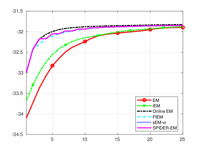
Refer to caption
Refer to caption
Figure 4: Monte Carlo approximation (computed over 4040 independent runs) of −𝔼⁡[W⁡(S^ℓ)]=−𝔼⁡[F∘𝖳⁡(S^ℓ)]-\mathbb{E}[\operatorname{W}(\widehat{S}_{\ell})]=-\mathbb{E}[F\circ\mathsf{T}(\widehat{S}_{\ell})] against the number of epochs. [left] Epochs 11 to 2525; [right] epochs 2525 to 150150.

On Figure 5 and Figure 6, for each of the algorithms FIEM, sEM-vr and SPIDER-EM, four different realizations of a path of the normalized likelihood are displayed as a function of the number of epochs. These four sets of curves differ from the selection of the sequence of mini-batches. The staircase behavior of the paths of sEM-vr and SPIDER-EM comes from the two successive kinds of epoch: one corresponds to a single optimization and a full scan of the data set and the other one corresponds to n/𝖻n/\mathsf{b} optimizations and the use of n/𝖻n/\mathsf{b} minibatches; the largest increase of W\operatorname{W} corresponds to the second type of epoch. Based on this criterion, the three algorithms are equivalent.

Refer to caption
Refer to caption
Figure 5: The objective function −W(S^ℓ)=−F∘𝖳(S^ℓ)-\operatorname{W}(\widehat{S}_{\ell})=-F\circ\mathsf{T}(\widehat{S}_{\ell}) against the number of epochs along two (left, right) independent runs of FIEM, sEM-vr and SPIDER-EM. The first 2525 epochs are discarded.
Refer to caption
Refer to caption
Figure 6: The objective function −W(S^ℓ)=−F∘𝖳(S^ℓ)-\operatorname{W}(\widehat{S}_{\ell})=-F\circ\mathsf{T}(\widehat{S}_{\ell}) against the number of epochs along two (left,right) independent runs of FIEM, sEM-vr and SPIDER-EM. The first 2525 epochs are discarded.

Figure 7 displays the evolution of the g=12g=12 iterates {α1,…,αg}\{\alpha_{1},\ldots,\alpha_{g}\} along a path of many algorithms. Figure 8 display the evolution of the p=20p=20 eigenvalues of the covariance matrix Σ\Sigma along a path of many algorithms. Here again, we observe a strong variability of Online EM when compared to the other algorithms.

Refer to caption
Figure 7: Evolution of the g=12g=12 iterates αk=(αk,1,…,αk,g)\alpha_{k}=(\alpha_{k,1},\ldots,\alpha_{k,g}) against the number of epochs, for EM, iEM and Online EM on the top from left to right; FIEM, sEM-vr and SPIDER-EM on the bottom from left ro right.
Refer to caption
Figure 8: Evolution of the p=20p=20 eigenvalues of the iterates {Σℓ,ℓ≥0}\{\Sigma_{\ell},\ell\geq 0\} against the number of epochs ℓ\ell, for EM, iEM and Online EM on the top from left to right; FIEM, sEM-vr and SPIDER-EM on the bottom from left ro right.

Figure 9 and Figure 10 display 4040 independent realizations of the squared norm of the mean field hh as a function of the number of epochs for different algorithms. It may be seen that Online EM has a strong variability and FIEM, sEM-vr, SPIDER-EM succeed in reducing this variability. FIEM converges more rapidly than iEM, and they achieve the same level of accuracy (here not better than 10−610^{-6}). sEM-vr and SPIDER-EM have the same level of accuracy, which is most often far smaller than the one reached by FIEM (more than 75%75\% of the paths reached an accuracy level of 10−1010^{-10} after 150150 epochs). Based on this criterion, we will definitively advocate the use of sEM-vr or SPIDER-EM when compared to iEM, Online EM and FIEM.

Refer to caption
Refer to caption
Refer to caption
Figure 9: [left] We display 4040 independent realizations of the squared norm of the mean field ℓ↦‖h⁡(S^ℓ)‖2\ell\mapsto\|h(\widehat{S}_{\ell})\|^{2} as a function of the number of epochs, along a iEM path. [center] same analysis for Online EM. [right] same analysis for FIEM.
Refer to caption
Refer to caption
Figure 10: [left] We display 4040 independent realizations of the squared norm of the mean field ℓ↦‖h⁡(S^ℓ)‖2\ell\mapsto\|h(\widehat{S}_{\ell})\|^{2} as a function of the number of epochs, along a sEM-vr path. [right] same analysis for SPIDER-EM.

Figure 11 and Figure 12 display the boxplots of 4040 independent realizations of ‖h⁡(S^ℓ)‖2\|h(\widehat{S}_{\ell})\|^{2} at time in {20,40,60,80,110}\{20,40,60,80,110\} epochs for different algorithms. In Figure 12, Online EM is not displayed since it is too large (compare the third plot on Figure 11 and the first one on Figure 12). The quantities {‖h⁡(S^ℓ)‖2,ℓ≥0}\{\|h(\widehat{S}_{\ell})\|^{2},\ell\geq 0\} are the key informations for deriving the complexity bounds in Theorem 2. The plots below show again that for small, medium and large values of the number of epochs kk, sEM-vr and SPIDER-EM provide the best results.

Refer to caption
Refer to caption
Refer to caption
Figure 11: Boxplots of 4040 independent points of ‖h⁡(S^ℓ)‖2\|h(\widehat{S}_{\ell})\|^{2} [left] at time 2020 epochs; [center] at time 4040 epochs; [right] at time 6060 epochs. The outliers are removed.
Refer to caption
Refer to caption
Refer to caption
Figure 12: Boxplots of 4040 independent points of ‖h⁡(S^ℓ)‖2\|h(\widehat{S}_{\ell})\|^{2} [left] at time 6060 epochs; [center] at time 8080 epochs; [right] at time 110110 epochs. The outliers are removed.