Spatio-temporal chaos of one-dimensional thin elastic layer with the rate-and-state friction law
Abstract
Independent of specific local features, global spatio-temporal structures in diverse phenomena around bifurcation points are described by the complex Ginzburg-Landau equation (CGLE) derived using the reductive perturbation method, which includes prediction of spatio-temporal chaos. The generality in the CGLE scheme includes oscillatory instability in slip behavior between stable and unstable regimes. Such slip transitions accompanying spatio-temporal chaos is expected for frictional interfaces of a thin elastic layer made of soft solids, such as rubber or gel, where especially chaotic behavior may be easily discovered due to their compliance. Slow earthquakes observed in the aseismic-to-seismogenic transition zone along a subducting plate are also potential candidates. This article focuses on the common properties of slip oscillatory instability from the viewpoint of a CGLE approach by introducing a drastically simplified model of an elastic body with a thin layer, whose local expression in space and time allows us to employ conventional reduction methods. Special attention is paid to incorporate a rate-and-state friction law supported by microscopic mechanisms beyond the Coulomb friction law. We discuss similarities and discrepancies in the oscillatory instability observed or predicted in soft matter or a slow earthquake.
I Introduction
Slip instability is ubiquitously found in a rich variety of phenomena Strogatz 2018; Rice and Ruina 1983. Indeed, we quite often encounter examples in daily life. For instance, the fascinating tones created by musical string instruments such as violins arise from stick-slip motion Fletcher and Rossing 1998. Another example is vehicles equipped with tires, where suppression of oscillatory instability is necessary to secure safety Persson 1997. The last important example given here is earthquakes Marone and Scholz 1988; Scholz 2002. Megathrust earthquakes occur in locked faults on subducting tectonic plates by suddenly releasing elastic energy stored by plate motion. Such slip instability emerges at the interface in the elastic body, and thus it is necessary to focus on the interfacial balance between friction and elasticity, in order to gain insights into the underlying physics.
Unstable slip motion may be generally involved in highly or weakly nonlinear components. This article focuses on weak nonlinearity around bifurcation points. By doing so, we construct a complex Ginzburg-Landau equation (CGLE) Kuramoto 1984; Aranson and Kramer 2002; Sugiura et al. 2014 that extracts common global structures without relying on specific microscopic features. It is worth noting that the CGLE offers a generic methodology applicable not only to slip instability, but also to instabilities near bifurcation points, such as transitions found in superconductivity, liquid crystals, Bernard convection, and Taylor vortices Kuramoto 1984; Aranson and Kramer 2002. The general framework of the CGLE is derived through the reductive perturbation method, which provides a simple description with a few degrees of freedom and parameters by eliminating fast variables in the original governing equations.
Our main interest is chaotic behavior manifesting in the weakly nonlinear slip instability around bifurcation points. This is one of the possible phenomena predicted by the CGLE framework, but the relevance of the chaos to slip instability at an interface of elastic media is still elusive. Systems made from rubber and gel would become feasible candidates exhibiting spatio-temporal chaos in laboratory experiments if an appropriate soft elastic solid is chosen from elastics with a broad range of compliance Baumberger and Caroli 2006; Baumberger et al. 2002; Yamamoto et al. 2014; Maegawa et al. 2016; Ben-David et al. 2010. Indeed, flexibility is a key parameter because distinctly heterogeneous stick-slip motions have been observed between a hard PMMA block and soft PDMS gels Yamaguchi et al. 2011. Recall here the rate-and-state friction (RSF) law discovered in rocks. The friction law acting on an interface even of a soft elastic solid is quite often of the RSF law family. Therefore, not only soft solids like gels, but also rigid materials such as rocks of importance to geoscience, are within the scope of the RSF law Baumberger and Caroli 2006. In fact, this study was inspired by slow earthquakes observed in subduction zones Obara 2002; Obara and Kato 2016. While regular or megathrust earthquakes accompany the high nonlinearity very far from the bifurcation point Marone and Scholz 1988, slow earthquakes could have common properties described by weakly nonlinear analyses because they occur in the transition zone between a locked and continuously creeping fault, which is reminiscent of the system parameter varying across the bifurcation point.
This paper discusses our analytical and numerical findings in the context of the CGLE based on weakly nonlinear analyses of a thin layer elastic body with the RSF law. The analyses are constructed through the reductive perturbation method Kuramoto 1984 that simplifies the original governing equation. This simplification is more than an approximation because it finds the universal features that become manifest through the elimination of specific local properties. In sec. II, we first introduce a thin elastic layer model under the RSF law. In sec. III, linear and weakly non-linear analyses are applied near the bifurcation point to show that the slow and global structures are represented by the CGLE, which may display spatio-temporal chaos due to Benjamin-Feir (BF) instability. Section IV demonstrates a numerical simulation, where time evolution is obeyed by the original governing equation before the reductive perturbation method, and then compares the results with the analytical calculations. An interesting point is that the size distribution of slip events numerically obtained for the chaotic regime is exponential, invoking the cumulative distribution of the seismic energy rate reported for slow earthquakes Yabe and Ide 2014. In sec. V, we consider the results of soft material experiments and those for slow earthquakes in light of the CGLE. Section VI concludes this study.
II Thin layer model with the RSF law
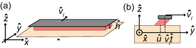
We begin with an introduction to an elastic thin layer system. A flat plate or sheet with thickness is placed on an - plane, and the -axis points upward so as to meet with the right-handed coordinate [see Fig. 1 (a)]. Friction acts on the bottom interface. The top boundary is dragged with constant loading velocity along the -axis, as shown in Fig. 1 (b). The layer is sheared and displaced along the -axis, to which the -axis is perpendicular. That is, we consider mode III, where displacements denoted by are uniform for the -component, so that we can deal with the system as one-dimensional and spanning the -direction.
Let us now move on to the governing equation. The elasticity is expressed by Navier’s equation. When the thickness of the elastic layer is small enough, imposing the boundary condition on Navier’s equation simplifies the equation of motion for the thin layer (see Appendix F) as
| (1) |
where , , , , , and denote the time, mass density, shear modulus for the elastic body, friction coefficient, normal stress, and velocity along the -axis, respectively. On the right side, the first two terms for the elastic force are derived from the continuum body model for the thin layer, where the interaction range is finite and is scaled by the thickness . The restoring force for the global inhomogeneous deformation along the -axis is replaced with the operator (), which serves as the local coupling. In addition, the top boundary condition emerges as loading in the second term. The last term is the friction that obeys the RSF law Kawamura et al. 2012; Ranjith and Rice 1999; Rathbun and Marone 2013, which acts on the bottom boundary interface with magnitude . The RSF law is commonly exploited to describe rock friction Morrow et al. 2017; Marone 1998, and is also known to be readily applicable to other materials, as seen in the literature Heslot et al. 1994; Baumberger and Caroli 2006. In addition, it is often used to describe regular Scholz 1998 and slow Shibazaki et al. 2012 earthquakes. Further, the RSF law friction model has been known to serve as the premise of slip instability related to nonlinear dynamics, including chaotic dynamics Viesca 2016a; Viesca 2016b; Ranjith 2014; Brener et al. 2018. The constitutive law for the RSF is written as
| (2) |
where , and denotes a variable that represents the interface state depending on the slip history. As an evolution law, this paper adopts the slip law Rice and Ruina 1983; Gu et al. 1984,
| (3) |
because it provides a better description of a fairly symmetric response with the characteristic distance to a discontinuous increase or decrease in stress Ampuero and Rubin 2008. The RSF law gives the steady-state friction as
| (4) |
meaning that velocity weakening occurs for , while velocity strengthening occurs for . A Hopf bifurcation that induces unstable slip behavior is observed below around and , which are the main regions of interest for slow earthquakes.
In preparation for the reductive perturbation method, we recast Eqs. (II)-(3) as time evolution Eqs. (II)-(14):
where
| (12) | |||||
| (13) | |||||
| (14) |
with three dimensionless variables:
| (15) |
Note that, for compact notation, the units for length, time, and stress are introduced, respectively, as follows:
| (16) |
We use the dimensionless variables , ,, , , , . In addition, parameters associated with the physical properties are listed below:
| (17) |
where represents the coupling with the driving factor provided by the upper plate, is the distance from the velocity weakening point (), and is the elastic wave velocity in the idealized plate. Bear in mind that the first two parameters identify the sliding stability, although the last one turns out to be irrelevant. In the following discussion, we restrict ourselves to the region where remains positive, and thus, . In the positive condition, we may circumvent the nonanalytic point that might cause a numerical instability (see appendix A).

III complex Ginzburg-Landau equation
III.1 Hopf Bifurcation
We first determine a fixed point through a linear stability analysis without spatial coupling by setting in Eq. (II). The steady sliding is given by the solution to the stationary state :
| (18) |
We look at small deviations around the steady-state solution to linearize Eqs. (II)-(14) as
The eigenvalues of the matrix satisfy the characteristic equation . Under the assumption that the roots of the cubic equation are one real root and two complex roots , the real root is obtained as . This ensures that the directions irrelevant to the Hopf bifurcation are stable (see appendix B). In contrast, the bifurcation is signified by . At , when turns from a negative to a positive value, a supercritical Hopf bifurcation appears with the following velocity and angular frequency:
| (23) |
which agrees with previous results Rice and Ruina 1983. It is worth noting that only two crucial parameters and enter into the equation to determine the stability behavior. The parameter is the distance from the velocity-weakening point, while represents the effective spring constant. For Eq. (23) to represent real values, and , or , is required. As long as this condition persists, the Hopf bifurcation point always exists, and the non-oscillatory solution for is unstable.
III.2 CGLE
We move on to a weakly nonlinear analysis of Eqs. (II)-(14) to obtain the CGLE (32). Bear in mind that the CGLE includes (i) a weakly nonlinear term and (ii) spatial local coupling. As in Eq. (24), the governing equation is expanded in a power series with a finite order, which is referred to as “weakly nonlinear analysis.” Loading velocity is set close to a Hopf bifurcation point as to expand the original Eq. (II) in the Taylor series with the small deviation around the steady state:
| (24) |
where
The matrix is expanded in a series of together with the -th order given by replacing with in the matrix of Eq. (III.1). Here, we employ notation such as , with summations running over repeated indices. In accordance with expansions in the matrices, the eigenvalue is replaced with
A supercritical Hopf bifurcation is observed for , which Eq. (III.2) satisfies because we now just focus on . In addition, the diffusion (local coupling) term in the present system is specified by .
Taking the term up to the order with an appropriate procedure Kuramoto 1984 (see also appendix G), we arrive at the CGLE with the slow time variable :
| (32) |
Note that the complex-valued is associated with the original governing Eq. (II) through
| (33) |
where the right eigenvector for with eigenvalue = is given by
and the coefficients with complex values are
| (38) |
The time scale between and is separated enough for the slow variable to undergo an adiabatic change. Equation (32) is a general form for a CGLE obeying the slow variable . The universal spatio-temporal structures are captured by the squared or cubed term of in the weakly nonlinear regime. For example, the general form of Eq. (32) includes the Ginzburg-Landau equation with the real coefficients . This is very often exploited to phenomenologically discuss phase transition dynamics with a variational function (Landau free energy), during which a system develops towards a minimum point. In contrast, if , we encounter the nonlinear Schrdinger equation with Eq. (32) Aranson and Kramer 2002, where conservative nonlinear wave phenomena are found without a dissipation mechanism. The present system is between these regimes and identified with a combination of the complex coefficients and .
Before including spatial coupling, let us discuss the general role of the complex coefficient of the cubic term through a homogeneous example with , or equivalently, the one reduced to the Stuart-Landau equation. Qualitative features are grasped in the amplitude-phase representation by rephrasing Eq. (32) with :
| (39) | |||
| (40) |
where amplitude and phase are real numbers. Eq. (39) gives the steady solution , which implies that the solution to the original Eq. (II) oscillates with a finite amplitude. The cubic term in Eq. (32) provides the solution not obtained from the linear analysis with Eq. (III.1). In addition, a close inspection shows that a leading part of the angular frequency is determined by , but modified by [Eq. (40)]. Notably, the oscillation amplitude affects the angular frequency through a higher-order perturbation term.
III.3 Benjamin-Feir Instability
When (ii) spatial local coupling participates in Eq. (32), spatio-temporal chaos, referred to as the BF instability, emerges for
| (41) | |||||
where the spatial gradient of the phase distribution is enhanced. The BF instability appears when the gradient in the phase modifies the amplitude , and it can be intensified through Eq. (40). Indeed, in the original Eq. (II), we find that the coupling term appears in the time derivative of , not in . The coupling term does not smooth the phase but shrinks the amplitude when the phase advances more than those of neighboring locations; consequently, the BF instability may appear. From the positive nature of , and , the condition for the BF instability is reduced to
| (42) |
which separates the BF-stable and BF-unstable regions in the - plane, as shown in Fig. 2. The boundary curve exhibits a convex downward shape and diverges at . Along the lower thick line as a function of at a fixed small below the minimum point of the boundary curve, the system is always unstable from to in the absence of a sufficient restoring force. This is a remarkable result because it implies that chaotic behavior appears if the material is soft enough. In contrast, if is large enough, e.g., , the system may enter the BF-stable regime at an intermediate value of . We also use Eq. (42) to distinguish the BF stability from BF instability by coloring the boundary curves with red and black, respectively, on the phase diagram in Fig. 3.


IV Numerical results
We performed a numerical simulation using the original governing Eqs. (II)-(14) to verify the reductive perturbation predictions. Note that an auxiliary viscous friction linearly proportional to the relative velocity between adjacent segments was incorporated as the second component of Eq. (II) to suppress the numerical instability. Indeed, appendix G provides positive evidence that the appropriate viscous friction was not strong enough to alter the qualitative behavior.
An explicit scheme under a periodic boundary condition was employed. Bear in mind that, as mentioned earlier, the simulation was halted when the velocity took on an invalid value [gray circled dots in Fig. 3 (a)]. The simulation started at , when the initial condition was prepared from the homogeneous steady solution of Eqs. (12)-(14) with the addition of small spatio-temporal disturbances. Because a strong artifact from the initial random conditions is unfavorable, we waited for the system to settle, and then the numerical samples were collected (see appendix C for detailed conditions).
IV.1 Phase Diagram
Typical phase diagrams are given in Fig. 3 (a), (b), where Hopf-bifurcation points sweep along solid curves determined with Eq. (23). In fact, persistent oscillation is not seen below these curves. The black and red curves signify whether the BF instability is absent or present, respectively.
Yellow squares around the black curve in Fig. 3 (a) indicate regular oscillations, whose dynamic behavior is exemplified in Fig. 4 (a-i). The pattern that appeared was not propagation but rather almost uniform oscillation with gradual spatial variation of the oscillation phase. Incidentally, the translational symmetry of the pattern was broken as a consequence of the initial randomness. Additionally, Fig. 4 (a-i) shows the velocity cross section taken from the density diagram along the red broken dashed line. The velocity profile looks symmetric about the loading velocity (). More quantitative analyses are shown in Fig. 4 (a-iii) (bottom). The duration of time spent around the maxima or minima of was the longest, which means that has peaks near or .
In contrast, irregular oscillations were observed (green crosses) near the red curves in Fig. 4 (b). The typical behavior of irregular oscillation has instability at short wavelengths, as in Fig. 4 (b-i), (b-ii). The wave pattern propagated at the velocity indicated by the white triangular area, which corresponds to the sound speed. This irregular oscillation meets with an example of spatio-temporal chaos due to the BF instability, because the phase distributions have random spikes in Fig. 3 (b-ii). A velocity profile was also taken from the spatio-temporal density map along the red dashed line. Although the oscillations are centered at , amplitudes became smaller than those of Fig. 3 (i). This point is made clear by looking at in Fig. 3 (iii), where bimodal distributions are found. In addition, the duration time spent around the lowest velocity was longest for this condition. Thus, a peak around is found, and turns out to be asymmetric.
The other phase is a slip pulse discovered at the points marked by blue asterisks in Fig. 3 (b). In the parameter region, spatially localized domains with finite slip velocity propagated at the sound speed, as those have a slope comparable to that of the white triangular area at the lower left corner. The slip velocity distributions look like a power law, where a large number of events on the distribution was found at small . The qualitative condition for pulse occurrence is similar to that in previous studies, where the slip pulse was reported for the model with velocity weakening friction Hirano and Yamashita 2016; Ampuero and Rubin 2008.
Focusing attention on the irregular oscillation associated with the BF instability among these four types of characteristic dynamics, we look for common features shared with slow earthquakes, such as tectonic tremors or slow slip events. One of the noteworthy points is the event size distribution. The simulation was performed in a larger space and with longer duration to collect statistical data [see Fig. 5 (a) and appendix C for detailed conditions]. The slip behavior is exemplified in Fig. 5 (a), where an irregular oscillation is observed. Figure 5 (b) shows the asymmetric bimodal distribution of slip velocity with respect to the loading velocity .

IV.2 Event size distributions
One of the important indices is the cumulative distribution of separate slip events. To identify separate events on a continuous spatio-temporal map, we binarize the density plot separated by threshold velocity that distinguishes “slipping” for from “no slipping” for . The connected slipping domains on a spatio-temporal map, that is, the area enclosed by a contour line on a spatio-temporal diagram [see the white-gray domain in Fig. 5 (c) with , below which the regions are drawn in solid black], are considered as a single slip event size .
The number of observed slip events varies according to [Fig. 5 (d)]. For , all the areas are completely connected and counted as a single slip event, which does not make sense statistically. However, for , no slip event is detected over the whole spatio-temporal plane. In the range , we monitored the distribution of event size for various values. Figure 5 (d) has a single peak around .
The shapes of isolated slip event domains do not look like fractal structures. This fact is verified by looking at the consistency with the Mandelbrot conjecture, which states that, if Korczak’s empirical law holds, the number of the isolated domains is supposed to be associated with the contour fractal curves characterized by the Hurst exponent through Mandelbrot 1982; Mandelbrot and Van Ness 1968. In particular, this was discussed for the fractal contours drawn with fractional Brownian motion Matsushita et al. 1991. This is not, however, true in the present system. As a matter of fact, neither the appearance of Fig. 5 (c) nor the distribution in Fig. 5 (d) seem to provide exponents and .
The probability density function , with estimated from binarized plots like those in Fig. 5 (c), is shown in Fig. 5 (e). As changes, exponential decreases along the event size are maintained. We are also aware that it is unlike the power law. Such exponential distributions resemble the cumulative distributions of seismic energy rates observed in tectonic tremors associated with slow earthquakes Yabe and Ide 2014. The exponential distributions are meant to have their own characteristic sizes. Fitting the exponential decay on Fig. 5(e), we estimated the characteristic event sizes , which are plotted in Fig. 5 (f). In addition, Fig. 5(e) is rescaled with , as in Fig. 5 (g).
V Discussion
Numerical and analytical aspects are discussed in secs. III and IV, respectively. Let us first verify the agreement between them from the viewpoint of qualitative and quantitative consistencies.
The qualitative point is the distribution shape. Recall that the numerical event size displays the exponential distribution, where the temporal plots on the spatio-temporal plane are fairly periodic [see the right side profile of Fig. 4 (b-i)], but the spatial plots are disordered [see Fig. 4 (b-ii)]. To make the point clear, we address both the temporal and spatial aspects. Although the temporal period varies over the long term with spatio-temporal chaos, a periodic pattern is found, implying that the characteristic time may correspond to the temporal period . In contrast, the spatial profiles are disordered rather than periodic because the neighboring differences in phase are intensified due to the BF instability mechanism. Especially, the spatial correlations get lost in the finite distance , suggesting that the correlations decay in an exponential manner. Therefore, the characteristic time and length may be defined using the temporal period and correlation length, respectively. Because the event size is defined as its area (time length) on the spatio-temporal plane, it is a natural consequence if an event has the characteristic event size , for which the size distribution is exponential.
Let us next review the quantitative applicability. As shown in sec. III, the characteristic time should be comparable to . The characteristic length is estimated from the wavelength of the most unstable mode on the propagating wave solution (see appendix D):
| (43) |
These characteristics indicate that event sizes are estimated with only two parameters, and . Setting the parameter values as and , employed in Fig. 5, we estimated the event size with and . The analytically estimated event size is on the same order of the size obtained from the numerical results in Fig. 5 (f). Thus, the analytical results with the CGLE show qualitatively and quantitatively excellent agreement with those of the numerical simulation.
A verification by laboratory experiments is necessary to determine the CGLE validity. Guided by Fig. 3 and Eq. (42), the slip mode becomes chaotic for small values of , which indicates that soft solids such as rubber and gel are promising materials for laboratory experiments. In a soft material sheet made from gels Baumberger et al. 2002; Baumberger and Caroli 2006; Yamaguchi et al. 2009; Baumberger et al. 2003; dum a, the estimated values for m and s would cause irregular slip due to the BF instability (see Table I in appendix E).. Although the characteristic length is slightly large, the experimental conditions fall into the feasible length and timescale of the observation for the BF instability by adding some modifications, such as different values for the rigidity, thickness, and loading speed. In addition to gels, rubber sheets ( Pa) with a thickness on the order of millimeters ( m) are also promising candidates because they have m and s.
In addition, let us here remark on the relation between the elasticity and the thickness. We are aware that the thickness is one of the important parameters because the elastic interaction has a range comparable to that of the thickness. Probably two limiting cases have been investigated most frequently: a thin layer or semi-infinite elastic half-space. However, we are not sure if the elastic-interaction range can alter the qualitative observations. In soft solids like rubber and gels, the thickness is rather easy to adjust so as to evaluate both thin and thick plates, whereas the present mathematical model constructed in the thin layer deals only with local coupling. The pertinent phenomena do not seem to have been observed yet at the laboratory scale, but the conditions described above would offer feasible projects.
Other practical applications are brake pads Behrendt et al. 2011, windscreen wiper blades Lancioni et al. 2016, and tires Persson 1997, where a relatively high loading rate as well as a thin elastic body are present. In such cases, spatially synchronized oscillation is undesirable in terms of stability, and the introduction of the spatio-temporal chaos due to BF instability may prevent such coherent oscillation. We may also include the peeling dynamics of soft adhesives Dalbe et al. 2015; Dalbe et al. 2016, where micro-scale stick-slip motion occurs, as a possible candidate for our analysis.
We then move on to a discussion about slow earthquakes. Recent seismic observations Yabe and Ide 2014 have shown that the cumulative distribution of the seismic energy rate can be fitted well using an exponential distribution. As seen in Section IV.2, the CGLE around the BF instability closely reproduces this exponential feature, which is in “qualitative” agreement with the observed consequences Yabe and Ide 2014. However, a “quantitative” agreement has not been achieved. Indeed, when plausible parameters Kano et al. 2010; Liu and Rice 2005; Scholz 1998 are plugged into the CGLE, we encounter unrealistically huge scales for the characteristic length and time s (see Table I in appendix E). Nonetheless, we should not rush to the conclusion that the CGLE approach is not completely appropriate in the study of slow earthquakes, because the CGLE approach itself is a very general framework independent of the specific structure of the system. Tracing back the derivation with the reductive perturbation method, the quantitative difficulty begins at Eq. (23), where the critical velocity is too low to meet with an appropriate oscillation period, as seen from . Thus, the primary modification should lie in a starting point around Eqs. (II)-(14) rather than the coupling term because Eq. (23) is a result obtained as an independent oscillator. This means that improvement from the local to nonlocal coupling Tanaka and Kuramoto 2003 is not enough to reproduce the realistic order estimate, although the thin layer is certainly a useful approximation. Alternatively, we arrive at the other possible candidates to improve the situation. Faster oscillation may be triggered by additional hidden variables, different from the elastic origin. For instance, recent observations reveal that fluid migration and precipitation of dissolved chemicals may control slow earthquakes Audet and Bürgmann 2014. They could bridge the quantitative gap while retaining the quantitative manner because the spatio-temporal chaos due to the BF instability derived from the general framework of the CGLE maintains an exponential dependence.
In addition to slow earthquakes, we suggest possible applications of our model to other geologically meaningful regimes. Such situations can be realized with increased loading velocity. Indeed, 1 m/s around the onset velocity of ordinary earthquakes that start to release seismic waves provides m or even a smaller order of magnitude for smaller . This implies that chaotic slip may occur inside faults on a subducting plate.
VI Concluding Remarks and Perspectives
We have discussed the application of the CGLE to the oscillatory instability observed in the thin layer model with the RSF law. The CGLE has a long history of being employed as a successful framework near the bifurcation (transition) points for various phenomena. Thus, this approach could embrace a diverse range of unstable interface systems.
Our analytical and numerical studies have primarily investigated the BF instability leading to chaotic behavior in light of the CGLE, and then we applied it to two notable cases in the main text: soft matter and slow earthquakes. To our knowledge, pertinent laboratory experiments with soft solids have not been reported. Instead, we have proposed feasible conditions for experiments with rubber or gel. A close inspection of the - diagram in Fig. 2 implies that soft solids are promising for verifying chaotic behavior in laboratory experiments due to their small compliance. One of the authors revealed the subsonic to intersonic transition in sliding friction of silicone gels Yashiki et al. 2020. According to the proposal in our study, friction of soft solids can exhibit spatio-temporal chaos with a loading velocity on the order of 10-2 m/s or higher. Such chaotic behavior may prevent tires from entering undesirable oscillatory synchronization for the practical purpose of braking. We emphasize that high-speed friction of soft matter should contain rich and fruitful physical phenomena to be investigated.
Slow earthquakes are also considered as an applicable issue. Comparing the observations of slow earthquakes with the analytical and numerical results, we can discover the qualitative coincidence of the exponential dependence of event size, whereas the quantitative estimates provide different results. The discrepancy arises from the fact that the present model lacks potentially crucial elements, such as heterogeneity or pore fluid pressure. Modifications by incorporating these elements could improve the quantitative gap without changing the qualitative aspects. This speculation is reasonable because the exponential distribution of slip event size is predicted by the BF instability mechanism derived from the general framework of the CGLE. Considering the broad ranging applicability of the CGLE, further studies based on the CGLE are expected to contribute to the understanding of slow earthquakes, as well as the slip instability occurring in soft matter.
Acknowledgment
This work was supported by the Japan Society for the Promotion of Science (JSPS), KAKENHI Grants JP16K13866, JP16H06478, JP19H05403, and JP21H05201. This work was also supported by JSPS and PAN under the Japan-Poland Research Cooperative Program “Spatio-temporal patterns of elements driven by self-generated, geometrically constrained flows,” and the cooperative research of “Network Joint Research Center for Materials and Devices” with Hokkaido University (Nos. 20161033, 20171033, and 20181048).
Appendix
A. Constraints on the sign of
It should be noted that, when , Eqs. (13) and (14) are not analytic. We tried several modifications of Eqs. (13) and (14) to avoid the non-analytic behavior near , especially to stabilize the numerical calculation. However, violent oscillation appeared, even after modifications, when changed its sign. Resolving this situation is beyond the scope of this study. Thus, we analytically and numerically restricted ourselves to . If became 0 or negative, the numerical simulation was halted.
B. Linear analysis
When a cubic equation has one real root, , and two complex roots, , it is written as
| (44) |
Comparing the characteristic equation reduced to with Eq. (44), we obtained
| (45) | |||||
| (46) | |||||
| (47) |
The parameter region and finds the critical velocity and angular frequency, respectively, in Eq. (23), as in the main text.
In contrast, if , oscillation does not appear in any sliding velocity . Also, if , oscillation emerges for any positive sliding velocity . The reductive perturbation method cannot be applied near the bifurcation point in either case (see also Fig. 2), but they are not of interest here.
C. Numerical setup
An explicit scheme under a periodic boundary condition was employed in the numerical simulations. The system was discretized with sizes and . In addition, the dimensionless parameters , , , and were used in Figs.3 and 4. The simulation was halted when the velocity assumed an invalid value, or . Although a time evolution that obeys the CGLE is deterministic, random initial conditions were generated by adding small disturbances to the homogeneous steady solution of Eqs. (II)-(14). In Figs. 3 and 5, the system sizes were 204.8 and 409.6, respectively.
Each simulation started at from a random initial condition. Because a strong artifact due to the initial condition is unfavorable, we waited for the system to settle. In Fig. 3, data were collected after . The sampling was done with and to obtain 1024 1024 spatio-temporal data points. Similarly, for the simulation shown in Fig. 5, data were collected after . The sampling was done with and to obtain 2048 163,920 spatio-temporal data points.
The numerical codes can be obtained from dum b.
D. Instability wavelength
Numerical calculations performed with the original governing equation produced irregular oscillation with the parameters used, whereas the BF instability was predicted by the analytical study. Furthermore, it was revealed that the event size defined as the area with a threshold slip velocity exhibits an exponential distribution. This exponential distribution suggests that there is a typical event size , and is written with a typical time and length . As discussed in sec. III, the oscillation period is comparable to , and the analytical estimate leads to . In contrast, the typical spatial size is estimated by the correlation length on the BF instability. To give a specific analytical expression for , we here turn back to the CGLE (32): The solution of the equation describes a propagating wave:
| (48) |
and
| (49) |
The solution exists for or with , where
| (50) |
Moreover, for the propagating wave to be stable against infinitesimal perturbations, we require an additional condition:
| (51) |
When , even homogeneous oscillation becomes unstable against infinitesimal perturbation, namely the BF instability. Specifically, the most unstable wavelength [Eq. (43)] is written as
| (52) |
Note that the typical spatial size is estimated from the most unstable wavelength. Eventually, we arrive at the analytical estimate for with , Eq. (23), and Eq. (52).
When the value used for the numerical simulation in Fig. 5 is inserted, , , and .
| gel | rubber | slow EQ | |
|---|---|---|---|
| kg/m3 | kg/m3 | kg/m3 | |
| N/m2 | N/m2 | N/m2 | |
| N/m2 | N/m2 | N/m2 | |
| N/m2 | N/m2 | N/m2 | |
| m/s | m/s | m/s | |
| m | m | m | |
| s | s | s | |
| 10-2 s | 10-3 s | 107 s | |
| 10-1 m | 10-2 m | 1019 m |
E. Order estimation of parameters
We estimated the order of and for soft matter or slow earthquakes. By referring to the parameters relevant to laboratory experiments with soft matter like gels Yamaguchi et al. 2011; Yamaguchi et al. 2016; Baumberger et al. 2002; Baumberger and Caroli 2006 or actual earthquakes Kano et al. 2010; Liu and Rice 2005; Scholz 1998, we estimated the order of parameters listed in Table I using the following approximations:
| (53) |
In addition, the following assumptions were applied for the soft matter experiments and the tectonic plate:
In laboratory experiments, we indirectly obtained from the other readings. For Table I, was adjusted to be close to the bifurcation point.
The thickness was chosen to satisfy
| (54) |
which justifies the thin layer elastic model with local coupling. In addition, although can be estimated from and using Eq. (23), we instead suppose .
The table leads to the conclusions that we could observe spatio-temporal chaos related to the present model in laboratory experiments Yamaguchi et al. 2011; Yamaguchi et al. 2016; Baumberger et al. 2002; Baumberger and Caroli 2006, but the order estimate does not show any quantitative agreement with results for geological phenomena.
F. Derivation of the BK model
The celebrated Burridge-Knopoff (BK) model Burridge and Knopoff 1967; Clancy and Corcoran 2006; Thøgersen et al. 2019; Thøgersen et al. 2021 consists of an array of rigid blocks that are driven in the same direction by elastic springs attached with the driving plate. In addition, adjacent blocks are connected with another kind of springs. The BK model was originally proposed using rigid discrete elements Burridge and Knopoff 1967 and has been criticized as an essentially discrete model Rice 1983. However, one can derive it by discretizing an elastic continuum subject to slow and long-wavelength deformation. Some attempts have been given in Clancy and Corcoran 2006; Thøgersen et al. 2021. Here we derive the BK model in a slightly different manner so as to clarify the validity and limitations of the model.
We start from the analytical solution given in the literature Rice and Ruina 1983, which is the relation between the shear stress and the displacement on the interface between two elastic plates of finite thickness .
| (55) | ||||
| (56) |
where denotes the elastic wave velocity. Here we assume that and and perform Taylor expansion with respect to these variables. Note that the Fourier transform is performed from and to and , respectively, and the superscript ∗ indicates variables after each transformation. We need to assume unless or .
Ignoring the higher-order terms in Eq. (56) and going back to the real spacetime, we arrive at the local expression for the shear stress and displacement:
| (57) |
Because this shear stress must balance with the friction, one obtains the following equation:
| (58) |
This reduces to Eq. (II) by changing the variables as follows: , , , and .
G. Derivation of CGLE
CGLE (Eq. (32)) is derived from a model of a thin elastic layer that incorporates a rate-and-state friction law (Eqs. (II)-(14)). Our derivation closely follows the scheme demonstrated in the reference Kuramoto 1984.
We first consider given equations without spatial coupling. Starting from following derivatives:
and the steady state solutions:
| (59) |
the following expressions are obtained at the steady state:
| (60) |
Loading velocity is set close to Hopf bifurcation point as . Expanding Eq. (G. Derivation of CGLE)-(G. Derivation of CGLE), by noting
| (61) |
up to the first order of , we have
| (62) |
The fluctuation around the steady state, obeys
| (63) |
where
The eigenvalue is expanded according to the leading order of as
| (67) |
where
| (68) |
and are right and left eigenvector for , while have following components:
The eigenvalues of are and where and . indicates that the corresponding direction in the phase space is stable against perturbations. By contrast, have zero real part. Indeed, the eigenvalue space for , become unstable at the Hopf bifurcation point. The right eigenvector corresponding for is
| (75) |
while the left eigenvector for is
| (76) |
where is a normalization factor to satisfy and
| (77) |
Using these expressions, one can obtain as:
| (78) |
We can take the real and imaginary parts of , which are relevant for the analysis related with BF instability, as
| (79) |
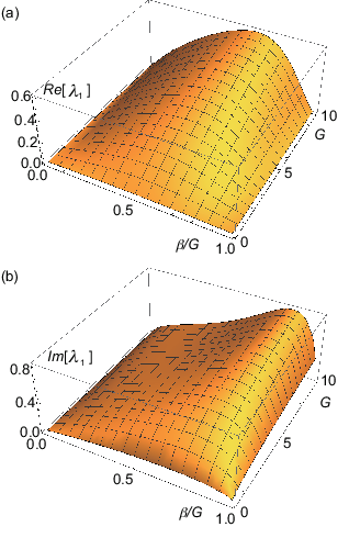
represents the growth rate of oscillation amplitude, and indicates that the steady state solution is not stable when . As shown in Fig. 6, is always positive in , and .
The higher order contribution of is necessary to converge the amplitude of destablized oscillation, and is included in the coefficient :
| (80) |
where
| (81) |
For the calculation, one should use the following matrices to calculate :
and
For =0,
and other second order and third order derivatives are zero. From Eq. (G. Derivation of CGLE), we obtain,
Inserting the components of the eigenvector ,
Then, and leads,
Thus, we obtain vector components for the following expressions as:
Collecting these resulting expressions,
and finally,
| (106) |
has the following real and imaginary parts:
| (107) |
| (108) |
From and , the oscillation amplitude, , is given as:
| (109) |
In addition, a part of the expression included in the condition of BF instability (Eq. (41)) is given as:
| (110) |
Based on the analyses on the spatially homogeneous situation, we then include the local diffusional coupling. The original equations to be considered are Eqs. (II)-(14), but the auxiliary viscose friction is additionally included in to estimate the impact on the dynamics. The complex diffusion constant is
From eigenvectors shown in Eqs. (75), (76),
| (111) |
where the real part and imaginary parts are
and
| (112) |
With , the expressions are simplified as:
| (113) |
The condition for the Benjamin-Feir instability with is
| (114) |
From and , the condition for Benjamin-Feir instability is
or equivalently,
| (115) |
References
- Strogatz (2018) S. Strogatz, Nonlinear Dynamics and Chaos (WestView, 2001), 1st ed.
- Rice and Ruina (1983) J. R. Rice and a. L. Ruina, Stability of Steady Frictional Slipping, J. Appl. Mech. 50, 343 (1983).
- Fletcher and Rossing (1998) N. H. Fletcher and T. D. Rossing, The Physics of Musical Instruments (Springer New York, New York, NY, 1998).
- Persson (1997) B. N. J. Persson, Sliding Friction: Physical Principles and Applications (Springer Series in Nanoscience and Technology, 1), NanoScience and Technology (Springer Berlin Heidelberg, Berlin, Heidelberg, 1997).
- Marone and Scholz (1988) C. Marone and C. H. Scholz, The depth of seismic faulting and the upper transition from stable to unstable slip regimes, Geophys. Res. Lett. 15, 621 (1988).
- Scholz (2002) C. H. Scholz, The Mechanics of Earthquakes and Faulting, 2nd ed. (Cambridge University Press, Cambridge, 2002).
- Kuramoto (1984) Y. Kuramoto, Chemical Oscillations, Waves, and Turbulence, Springer Series in Synergetics, Vol. 19 (Springer Berlin Heidelberg, Berlin, Heidelberg, 1984).
- Aranson and Kramer (2002) I. S. Aranson and L. Kramer, The world of the complex Ginzburg-Landau equation, Rev. Mod. Phys. 74, 99 (2002).
- Sugiura et al. (2014) N. Sugiura, T. Hori, and Y. Kawamura, Synchronization of coupled stick-slip oscillators, Nonlinear Process. Geophys. 21, 251 (2014).
- Baumberger and Caroli (2006) T. Baumberger and C. Caroli, Solid friction from stick-slip down to pinning and aging, Adv. Phys. 55, 279 (2006).
- Baumberger et al. (2002) T. Baumberger, C. Caroli, and O. Ronsin, Self-Healing Slip Pulses along a Gel/Glass Interface, Phys. Rev. Lett. 88, 075509 (2002).
- Yamamoto et al. (2014) T. Yamamoto, T. Kurokawa, J. Ahmed, G. Kamita, S. Yashima, Y. Furukawa, Y. Ota, H. Furukawa, and J. P. Gong, In situ observation of a hydrogel-glass interface during sliding friction, Soft Matter 10, 5589 (2014).
- Maegawa et al. (2016) S. Maegawa, F. Itoigawa, and T. Nakamura, Dynamics in sliding friction of soft adhesive elastomer: Schallamach waves as a stress-relaxation mechanism, Tribol. Int. 96, 23 (2016).
- Ben-David et al. (2010) O. Ben-David, S. M. Rubinstein, and J. Fineberg, Slip-stick and the evolution of frictional strength,Nature 463, 76 (2010).
- Yamaguchi et al. (2011) T. Yamaguchi, M. Morishita, M. Doi, T. Hori, H. Sakaguchi, and J. P. Ampuero, Gutenberg-Richter’s law in sliding friction of gels, J. Geophys. Res. Solid Earth 116, 1 (2011).
- Obara (2002) K. Obara, Nonvolcanic deep tremor associated with subduction in southwest Japan, Science 296, 1679 (2002).
- Obara and Kato (2016) K. Obara and A. Kato, Connecting slowearthquakes to huge earthquakes, Science 353, 253 (2016).
- Yabe and Ide (2014) S. Yabe and S. Ide, Spatial distribution of seismic energy rate of tectonic tremors in subduction zones, J. Geophys. Res. Solid Earth 119, 8171 (2014).
- Kawamura et al. (2012) H. Kawamura, T. Hatano, N. Kato, S. Biswas, and B. K. Chakrabarti, Statistical physics of fracture, friction, and earthquakes, Rev. Mod. Phys. 84, 839 (2012).
- Ranjith and Rice (1999) K. Ranjith and J. Rice, Stability of quasi-static slip in a single degree of freedom elastic system with rate and state dependent friction, J. Mech. Phys. Solids 47, 1207 (1999).
- Rathbun and Marone (2013) A. P. Rathbun and C. Marone, Symmetry and the critical slip distance in rate and state friction laws, J. Geophys. Res. Solid Earth 118, 3728 (2013).
- Morrow et al. (2017) C. A. Morrow, D. E. Moore, and D. A. Lockner, Frictional strength of wet and dry montmorillonite, J. Geophys. Res. Solid Earth 122, 3392 (2017).
- Marone (1998) C. Marone, Laboratory-Derived Friction Laws and Their Application To Seismic Faulting, Annu. Rev. Earth Planet. Sci. 26, 643 (1998).
- Heslot et al. (1994) F. Heslot, T. Baumberger, B. Perrin, B. Caroli, and C. Caroli, Creep, stick-slip, and dry-friction dynamics: Experiments and a heuristic model, Phys. Rev. E 49, 4973 (1994).
- Scholz (1998) C. H. Scholz, Earthquakes and friction laws, Nature 391, 37 (1998).
- Shibazaki et al. (2012) B. Shibazaki, K. Obara, T. Matsuzawa, and H. Hirose, Modeling of slow slip events along the deep subduction zone in the Kii Peninsula and Tokai regions, southwest Japan, J. Geophys. Res. Solid Earth 117, B06311 (2012).
- Viesca (2016a) R. C. Viesca, Stable and unstable development of an interfacial sliding instability, Phys. Rev. E 93, 060202 (2016a).
- Viesca (2016b) R. C. Viesca, Self-similar slip instability on interfaces with rate- and state-dependent friction, Proc. R. Soc. A: Math. Phys. Eng. Sci. 472, 20160254 (2016b).
- Ranjith (2014) K. Ranjith, Instabilities in Dynamic Anti-plane Sliding of an Elastic Layer on a Dissimilar Elastic Half-Space, J. Elast. 115, 47 (2014).
- Brener et al. (2018) E. A. Brener, M. Aldam, F. Barras, J. F. Molinari, and E. Bouchbinder, Unstable Slip Pulses and Earthquake Nucleation as a Nonequilibrium First-Order Phase Transition, Phys. Rev. Lett. 121, 234302 (2018).
- Gu et al. (1984) J.-C. Gu, J. R. Rice, A. L. Ruina, and S. T. Tse, Stability of quasi-static slip in a single degree of freedom elastic system with rate and state dependent friction, J. Mech. Phys. Solids 32, 167 (1984).
- Ampuero and Rubin (2008) J.-P. Ampuero and A. M. Rubin, Earthquake nucleation on rate and state faults - Aging and slip laws, J. Geophys. Res. 113, B01302 (2008).
- Hirano and Yamashita (2016) S. Hirano and T. Yamashita, Modeling of Interfacial Dynamic Slip Pulses with Slip-Weakening Friction, Bull. Seismol. Soc. Am. 106, 1628 (2016).
- Mandelbrot (1982) B. B. Mandelbrot, The fractal geometry of nature (Freeman, San Francisco, CA, 1982).
- Mandelbrot and Van Ness (1968) B. B. Mandelbrot and J. W. Van Ness, Fractional Brownian Motions, Fractional Noises and Applications, SIAM Rev. 10, 422 (1968).
- Matsushita et al. (1991) M. Matsushita, S. Ouchi, and K. Honda, On the Fractal Structure and Statistics of Contour Lineson a Self-Affine Surface, J. Phys. Soc. Jpn. 60, 2109 (1991).
- Yamaguchi et al. (2009) T. Yamaguchi, S. Ohmata, and M. Doi, Regular to chaotic transition of stick-slip motion in sliding friction of an adhesive gel-sheet, J. Condens. Matter Phys. 21, 205105 (2009).
- Baumberger et al. (2003) T. Baumberger, C. Caroli, and O. Ronsin, Self-healing slip pulses and the friction of gelatin gels, Euro. Phys. J. E 11, 85 (2003).
- dum (a) T. Fukudome, M. Otsuki, Y. Sawae, P. A. Selvadurai and T. Yamaguchi, in preaparation .
- Behrendt et al. (2011) J. Behrendt, C. Weiss, and N. P. Hoffmann, A numerical study on stick-slip motion of a brake pad in steady sliding, J. Sound Vib. 330, 636 (2011).
- Lancioni et al. (2016) G. Lancioni, S. Lenci, and U. Galvanetto, Dynamics of windscreen wiper blades: Squeal noise, reversal noise and chattering, Int. J. Non-Linear Mech. 80, 132 (2016).
- Dalbe et al. (2015) M.-J. Dalbe, P.-P. Cortet, M. Ciccotti, L. Vanel, and S. Santucci, Multiscale Stick-Slip Dynamics of Adhesive Tape Peeling, Phys. Rev. Lett. 115, 128301 (2015).
- Dalbe et al. (2016) M.-J. Dalbe, R. Villey, M. Ciccotti, S. Santucci, P.-P. Cortet, and L. Vanel, Inertial and stick-slip regimes of unstable adhesive tape peeling, Soft Matter 12, 4537 (2016).
- Kano et al. (2010) M. Kano, S. Miyazaki, K. Ito, and K. Hirahara, Estimation of Frictional Parameters and Initial Values of Simulation Variables Using an Adjoint Data Assimilation Method with Synthetic Afterslip Data, Zisin (J. Seismol. Soc. Jpn. 2nd ser.) 63, 57 (2010).
- Liu and Rice (2005) Y. Liu and J. R. Rice, Aseismic slip transients emerge spontaneously in three-dimensional rate and state modeling of subduction earthquake sequences, J. Geophys. Res. 110, B08307 (2005).
- Tanaka and Kuramoto (2003) D. Tanaka and Y. Kuramoto, Complex Ginzburg-Landau equation with nonlocal coupling, Phys. Rev. E 68, 026219 (2003).
- Audet and Bürgmann (2014) P. Audet and R. Bürgmann, Possible control of subduction zone slow-earthquake periodicity by silica enrichment, Nature 510, 389 (2014).
- Yashiki et al. (2020) T. Yashiki, T. Morita, Y. Sawae, and T. Yamaguchi, Subsonic to Intersonic Transition in Sliding Friction for Soft Solids, Phys. Rev. Lett. 124, 238001 (2020).
- dum (b) See https://arxiv.org/abs/2012.01799 and access Code and Data tab where one can access source codes to create Fig. 3 and Fig. 5.
- Yamaguchi et al. (2016) T. Yamaguchi, Y. Sawae, and S. M. Rubinstein, Effects of loading angles on stick-slip dynamics of soft sliders, Extreme Mech. Lett. 9, 331 (2016).
- Burridge and Knopoff (1967) R. Burridge and L. Knopoff, Model and theoretical seismicity, Bull. Seismol. Soc. Am. 57, 341 (1967).
- Clancy and Corcoran (2006) I. Clancy and D. Corcoran, Burridge-Knopoff model: Exploration of dynamic phases, Phys. Rev. E 73, 046115 (2006).
- Thøgersen et al. (2019) K. Thøgersen, H. A. Sveinsson, D. S. Amundsen, J. Scheibert, F. Renard, and A. Malthe-Sørenssen, Minimal model for slow, sub-Rayleigh, supershear, and unsteady rupture propagation along homogeneously loaded frictional interfaces, Phys. Rev. E 100, 043004 (2019).
- Thøgersen et al. (2021) K. Thøgersen, E. Aharonov, F. Barras, and F. Renard, Minimal model for the onset of slip pulses in frictional rupture, Phys. Rev. E 103, 052802 (2021) .
- Rice (1983) J. R. Rice, Spatio-temporal Complexity of Slip on a Fault, J. Geophys. Res. 98, 9885 (1993) .