Hydrodynamic Theory of the Connected Spectral Form Factor
Abstract
One manifestation of quantum chaos is a random-matrix-like fine-grained energy spectrum. Prior to the inverse level spacing time, random matrix theory predicts a ‘ramp’ of increasing variance in the connected part of the spectral form factor. However, in realistic quantum chaotic systems, the finite time dynamics of the spectral form factor is much richer, with the pure random matrix ramp appearing only at sufficiently late time. In this article, we present a hydrodynamic theory of the connected spectral form factor prior to the inverse level spacing time. We first derive a general formula for the spectral form factor of a system with almost-conserved sectors in terms of return probabilities and spectral form factors within each sector. Next we argue that the theory of fluctuating hydrodynamics can be adapted from the usual Schwinger-Keldysh contour to the periodic time setting needed for the spectral form factor, and we show explicitly that the general formula is recovered in the case of energy diffusion. We also initiate a study of interaction effects in this modified hydrodynamic framework and show how the Thouless time, defined as the time required for the spectral form factor to approach the pure random matrix result, is controlled by the slow hydrodynamics modes. We then extend the formalism to Floquet systems, where a ramp is expected but with a different coefficient, and we derive a crossover formula from the Hamiltonian ramp to the Floquet ramp when the Floquet drive is weak. Taken together, these results establish an effective field theory of chaotic spectral correlations which predicts the random matrix ramp at late time and computes corrections to it at earlier times.
I Introduction
There has been a surge of recent interest Haake 2010; Bohigas et al. 1984; Mehta 2004 in the statistics of energy levels of “chaotic” quantum systems. Quantum chaos in this loose sense is typically invoked when quantizing a classically chaotic system and in the context of quantum systems that effectively thermalize. It is widely believed that ensembles of such chaotic systems have the same Hamiltonian spectral statistics as ensembles of Gaussian Hermitian random matrices, with examples from nuclear systems Dyson 1962; Wigner and Griffin 1959 to condensed matter systems Bohigas and Giannoni 1984; Dubertrand and Müller 2016; Bertini et al. 2018 to holographic theories Cotler et al. 2017; Saad et al. 2019. One line of thought even proposes to take random-matrix-like spectral statistics as a definition of quantum chaos, which then denotes a super-class of physical systems that includes many-body systems like nuclear matter (which were Wigner’s motivation for introducing the random matrix ansatz) and quantized few-body systems (where the connection to classical chaos is clear). From this point of view, classical chaos still has an important relation to quantum chaos, but it is only directly relevant for a subset of all quantum chaotic systems with a recognizable semi-classical limit.
These ideas also raise a fundamental question: how do we tell which physical systems possess quantum chaos in the spectral sense? Of course, if we have access to the fine-grained energy levels then it is easy to check from the definition, but what if we only have access to more coarse-grained information (as is very often the case in experiment)? For example, thermalization is a widely observed phenomenon that is also closely associated with quantum chaos in the above loose sense, so one can wonder whether chaos in the sense of exhibiting thermalization implies chaos in the sense of random-matrix-like spectral statistics (and vice versa). In this paper, we argue that if an isolated quantum system thermalizes, then it possesses quantum chaos in the spectral sense.
We do this by building an effective description that predicts the apparent universality of random matrix spectral correlations and computes corrections to the pure random matrix answer in the presence of structure in the physical Hamiltonian. The idea of our approach is that corrections to pure random matrix behavior should be controlled by the slow “hydrodynamic” modes of the system since these are what distinguish a Hamiltonian with structure from one without. Then, starting from a proper effective theory of these slow modes, we propose a principled modification of that theory which predicts random matrix behavior at late time and can compute corrections to it at earlier times. Although one might have thought that these slow modes only control corrections to pure random matrix behavior, the same effective theory is able to produce the random matrix behavior itself. Thermalization is built into the approach from the start, since we assume that all other modes decay rapidly in time and the effective theory of the slow modes is generic in the sense of effective field theory.
To explain more precisely what our effective theory computes, we first need to specify what we mean by spectral correlations. Suppose is an ensemble of Hamiltonians depending on some random variables (“disorder”) collectively denoted . We say that the ensemble is random-matrix-like if the statistical properties of the eigenvalues of reproduce those of a Gaussian random matrix ensemble with the same symmetry. The spectral statistics of the ensemble can be defined using the density of energy eigenvalues, . The simplest object to consider is the ensemble averaged eigenvalue density, , but as reviewed below, this quantity depends on all the details of the random matrix ensemble and does not provide a universal signature. However, the ensemble averaged pair correlation, , is universal across a wide variety of ensembles (even non-Gaussian ones), so it provides a useful diagnostic of randomness in the spectrum.
However, such comparisons between the physical spectra of and the predictions of random matrix theory must be applied with care, since a particular chaotic quantum system will typically only have random matrix-like spectral correlations for energy levels that are sufficiently close in energy. This is because physical systems typically have structure in the Hamiltonian, such as constraints arising from spatial locality, which is not present in standard random matrix ensembles and which must be effectively washed out by the dynamics. The effective loss of structure can only happen at long times after the system has come to global equilibrium. For this reason, it is convenient to think about spectral correlations in the time domain by considering the Fourier transform of with respect to the relative energy . Then longer times correspond to increasingly closely spaced energy levels.
In this paper, we study the Fourier transformed pair correlation, which is known as the spectral form factor (SFF), and present a hydrodynamic theory of the intermediate time spectral properties of generic quantum chaotic systems. By hydrodynamics we mean the recently developed formal effective field theory that governs the slow modes of the system Dubovsky et al. 2012; Grozdanov and Polonyi 2015a; Haehl et al. 2018; Crossley et al. 2017; Jensen et al. 2018. The relevant modes control the late time behavior of the system as it approaches global equilibrium, and our theory makes a sharp connection between hydrodynamics and the spectral form factor. Moreover, symmetries and hydrodynamics are an inescapable part of the story because time-independent Hamiltonian systems always have at least time translation symmetry and energy conservation, so in a spatially local system there is always at least one slow mode. The hydrodynamic approach we develop predicts that the late time spectral correlations are random-matrix-like and gives quantitative tools to compute corrections to pure random matrix behavior at earlier times. As such, the theory we propose can be viewed as an effective field theory of chaotic spectral correlations.
Before proceeding, we briefly highlight the context of our work. There is a very large literature on quantum chaos extending back many decades. One key paper is Altshuler and Shklovskii 1986 which showed that the variance of the number of single particle energy levels in an energy window was random-matrix-like for energies smaller than the inverse Thouless time defined from particle diffusion. This time originally arose in the context of mesoscopic transport as a measure of the sensitivity of the system to boundary conditions, but it has come to refer to the timescale beyond which quantum dynamics looks random-matrix-like. Other prior investigations of the Thouless time in a many-body setting include Schiulaz et al. 2019; Gharibyan et al. 2018; Friedman et al. 2019; Altland and Bagrets 2018; Nosaka et al. 2018, with one result being that the Thouless time can depend on the observable used to define it. There are also a growing number of exact diagonalization studies and analytic results on many-body spectral statistics and spectral form factors including Bertini et al. 2018; Saad et al. 2019; García-García and Verbaarschot 2017; Altland and Sonner 2020. Roy and Prosen 2020 derives a similar formula to our 13. One useful recent review on various aspects of quantum chaos is D’Alessio et al. 2016.
To setup a more precise statement of our main results, we first review the basics of random matrix theory (RMT) and the observables of interest. After this short review, we outline our results at the end of the introduction and give a guide to the paper.
I.1 Random matrix theory and spectral form factor
A “single trace” random matrix ensemble is characterized by two pieces of data. The first datum is the type of matrix (orthogonal, unitary, symplectic) and corresponding Dyson index . In physical terms, this relates to the number and nature of antiunitary symmetries. The second datum is a potential , where we choose matrix with probability . These data give a joint probability for the eigenvalues equal to
| (1) |
where is a normalization.
This probability distribution can be conveniently interpreted in terms of a “Coulomb gas” of eigenvalues as follows. Eq. 1 has the form of a Boltzmann distribution at unit temperature for a gas of 1d particles at positions with logarithmic Coulomb interactions subject to an external potential Mehta 2004. In this way of thinking, the correlations of the density of particles/eigenvalues,
| (2) |
form a natural set of observables. The most basic of these observables is the density of states, , where the overline denotes an average over the random matrix ensemble. For example, in a Gaussian random matrix ensemble in which the potential is quadratic, this average is well approximated by the famous Wigner semi-circle law. However, the average density of states is non-universal since it depends on the potential . The simplest observable that probes spectral correlations and which does not depend strongly on is the 2-point function of the density, .
It is common Heusler et al. 2004; Brézin and Hikami 1997 to package this 2-point function into an object in the time domain called a spectral form factor (SFF), defined here to include a filter function ,
| (3) |
Very often we choose , which we call the SFF at inverse temperature . (In this paper is the Dyson index and is inverse temperature. is time and never temperature.) Another useful choice for is a Gaussian function zeroed in on a part of the spectrum of interest. The filtered SFF is then the ensemble average of the squared magnitude of the -component of the Fourier transform of ,
| (4) |
The SFF of a random matrix breaks into three regimes. First, a slope region, where Eq. 3 is dominated by the disconnected part of the 2-point function of . Once the system reaches the Thouless time when all macroscopic degrees of freedom have relaxed, we reach a new stage. This second state is the ramp, where the disorder-averaged SFF is linear in . In this regime the SFF is given by
| (5) |
The ramp continues until the Heisenberg time set by the inverse level spacing. At such long times, the off-diagonal terms in equation (3) average to zero and the SFF is a flat plateau. An example log-log plot of a random matrix SFF is shown in Fig. 1.

It is further useful to decompose the SFF into connected and disconnected pieces. In terms of the thermodynamic partition function evaluated at imaginary inverse temperature ,
| (6) |
the SFF is
| (7) |
where
| (8) |
and
| (9) |
Fig. 2 shows the very different behaviors of these two pieces of the SFF. The disconnected part is controlled just by the density of states, so we can more cleanly access the spectral correlations by focusing on the connected part.

I.2 Overview of results
Given this background and notation, we can now state our main results. We first fix some terminology used in the paper. The ramp typically refers to the linear in time part of the connected spectral form factor. In a many-body system of degrees of freedom with no symmetries or slow modes, the ramp is expected to onset after a short relatively short time of order .11 1 This is the time it takes for an exponentially decaying mode of the form to reach a suppressed amplitude provided the rate is not -dependent. The main topic of this article is the modification of the random matrix ramp due to slow modes and non-random matrix features of the system. One could conceivably speak about a ‘time-dependent ramp coefficient’, but we prefer to consider the time period prior to the pure random matrix ramp as distinct regime. In this view, there are four time periods: (1) the very early regime, prior to a time of order , when all the details matter, (2) the hydrodynamic regime, when the spectral form factor is determined by the symmetries and slow modes of the system, but is insensitive to other details, (3) the pure random matrix ramp regime, and (4) the plateau regime.
In this paper we study in detail the connected spectral form factor in the hydrodynamic regime (regime 2) and the pure random matrix ramp regime (regime 3). By contrast, the very early time regime (regime 1) is totally non-universal, and the very late time regime (regime 4) is straightforward to understand microscopically (albeit potentially mysterious from other points of view). We define the Thouless time to be the time it takes for the SFF to come close the pure random matrix ramp, i.e. the crossover time from regime 2 to regime 3. One of our key results is an expression relating the connected SFF to return probabilities (equations (13) and (15)), giving precise meaning to the notion that RMT behavior takes over when the system has had time to fully explore Hilbert space Schiulaz et al. 2019.
The remainder of the paper is organized as follows. In Section II we discuss the case of approximate symmetries, corresponding to slowly decaying modes, in general quantum mechanical terms. We show that the connected spectral form factor can be computed in terms of return probabilities for the slow modes. Next, in Section III we argue that the theory of fluctuating hydrodynamics, conventionally formulated on the Schwinger-Keldysh contour, can be adapted to the periodic time contour defining the spectral form factor. Focusing on the case of energy diffusion, we show that this “closed time path” (CTP) formalism, modified with periodic boundary conditions, recovers the ramp at late time and the return probability formula at intermediate time. Then, in Section IV we discuss in more detail the effects of interactions and study a partial resummation of perturbative diagrams. Next, in Section V, we study driven Floquet systems, deriving general formulas for their behavior, rederiving a number of known results, and correctly predicting the crossovers between different regimes of the Floquet drive.
II Nearly Block Hamiltonians
As discussed above, a particular quantum chaotic system will only approach the random matrix prediction at sufficiently late time. At earlier times, the presence of structure in the Hamiltonian typically implies a significant deviation from the pure random matrix result. In this section, we derive a general formula for the spectral form factor of such systems assuming a certain decomposition into weakly coupled random-matrix-like blocks. This section should be viewed as an introduction to the effects of slow modes on the spectral correlations, one in which the results can be obtained from physically transparent assumptions and elementary manipulations of quantum states. Later in Sec. III we will show how these results are recovered from our hydrodynamic effective theory.
So, suppose the Hamiltonian decomposes into two pieces, , such that breaks into decoupled blocks and causes transitions between the blocks. We take the -induced transitions to be slow and the blocks to be random-matrix-like. To compute (we will add the filter function later), we want to sum over all return amplitudes. Consider a basis for the Hilbert space labelled by the pair where denotes the block and indicates a basis vector within a block. Given an initial state , write its time development as
| (10) |
where is the probability to transition to sector after starting in sector (assumed to be independent of the within-sector label ) and is the normalized state in sector originating from . The return amplitude is
| (11) |
The SFF is assembled by summing these amplitudes, taking the squared magnitude, and then averaging over the ensemble. Now, since the dynamics within each sector is random matrix like at the timescales of interest, the diagonal terms should reduce to the within-sector SFF and the off-diagonal terms should be small,
| (12) |
Hence, the filtered SFF reduces to
| (13) |
When the individual blocks are random-matrix-like, then is just a linear ramp with a known coefficient, and the evaluation of the SFF reduces to summing over the return probabilities.
II.1 Path integral example
To understand the return probabilities in more detail and to introduce a useful rate-matrix formalism, consider the instructive example of a particle stuck in one of potential wells, in a kinematic space complicated enough such that the Hamiltonian within each well is well-approximated by a random matrix. The single almost-conserved quantity is an index ranging from to .

We can solve this using doubled-system wormhole techniques like those in Saad et al. 2019, reviewed in appendix A. As a first glimpse of this technology, imagine that the particle dynamics is governed by some classical action such that the trace of the time evolution operator is obtained from a path integral constructed from said action. The SFF is then obtained by doubling this path integral, with one copy for the forward time evolution and one copy for the backward time evolution. We will not need the details of this description, just some general properties. In particular, we will not keep track of the detailed dynamics within a well, but we will follow the dynamics of the discrete variable denoting which well the particle is in.
Now, the simplest solutions to the equations of motion in a doubled system are ones where is constant over the entire doubled contour. There are also solutions where is different on the two contours, but their contributions average to zero because of our assumption that the within-well dynamics is chaotic. Hence, the first rule is that the well index must agree between the two contours. This is analogous to Eq. (12). There are also tunneling events or instantons which take the system from well to well, and we can put all their probabilities into a transition rate matrix . Here denotes the energy at which the transition is happening. also has elements on the diagonals to make sure probability is conserved. Note that because these tunneling events happen on a doubled system, the pair of amplitudes, one from each copy of the system, naturally combine to form probabilities. It is these probabilities which are the matrix elements of . An illustration of one configuration which contributes to the path integral is given in figure 3. Note that is not a Hermitian matrix. It has all negative eigenvalues, except for one zero eigenvalue whose left eigenvector is corresponding to conservation of probability).
To get from the transition matrix to the SFF, the key point is that the same instanton gas that gives us the probability of transfer also shows up in a wormhole-like path integral calculation of the SFF. We start with out in a thermofield double (TFD) for the various approximately disconnected sectors of the Hamiltonian. At each timestep from to , there is some amplitude (probability from the point of view of a single copy of the system) that the system will go from sector to sector . This is just . Multiplying over all timesteps, and requiring that the doubled system start and end in the same sector gives
| (14) |
This means that the SFF is given by
| (15) |
where the in front still comes from an overall displacement of one side relative to the other. Relative to the pure random matrix result, the coefficient in (15) starts out as for wells and goes down to at long time. It is also worth noting that if there are truly conserved quantities, formula (15) will still give correct results. One interpretation of (15) is as a precise version of the claim that one gets the pure RMT result once enough time has passed for a state to explore all of Hilbert space Schiulaz et al. 2019.
To illustrate the working of formula (15), suppose we have a random Hermitian matrix of the following form: a complex symmetric matrix, decomposed into blocks, with elements of variance on the diagonal blocks and variance on the off-diagonal blocks. We can use Fermi’s Golden Rule to get transition rates: the squared matrix element is just and the density of states is (semi-circle law), so the overall rate is . Figure 4 shows three increasingly complicated scenarios. In the first one, there are two blocks connected with . In the second, there are three blocks of different sizes. In the third, a chain of blocks where only neighboring blocks are connected. This is analogous to a particle slowly diffusing, where its position is approximately conserved. In each graph, we show the realized ratio of the connected SFF to the predicted single block SFF, and also .


III Hydrodynamics
We now turn to the main topic of this paper, the hydrodynamic theory of the connected spectral form factor. Let us quickly recap why hydrodyamics is relevant. As the theory of a system’s slow modes, hydrodynamics provides a natural framework in which to evaluate the return probabilities entering the general formula in equations (13) and (15). One might have thought that the late time pure random matrix ramp must still be input by hand, as in the argument in the previous section. However, we will see that the theory developed in this section actually predicts the late time pure random matrix ramp as well. We first motivate the discussion using energy diffusion, then describe our theory in detail in a series of subsections.
III.1 Energy diffusion and almost conserved quantities
Energy diffusion is interesting not only as a simple test case, but because it is very generic: any spatially local Hamiltonian system which thermalizes and which does not have additional conserved quantities (the generic case, e.g. due to disorder breaking translation symmetry) is described by this theory at long time/distance. This class of systems fits the previous setting because in the limit of large volume at a fixed time , such a hydrodynamic system has an extensive set of approximate conservation laws.
As a first step, let us count the number of approximately conserved charges. For linear diffusion, the amplitude of a long-wavelength energy fluctuation with wavevector decays at rate , where is the energy diffusion constant. In this case, all modes with wavevector less than have not appreciably decayed up to time . In spatial dimension , the number of such modes is
| (16) |
which is extensive in the system size . Hence, since the amplitude of each energy fluctuation with wavevector is almost conserved, we have an extensive set of almost conserved quantities. The approximately decoupled sectors are then labelled by a choice of amplitude for each mode with . Moreover, within a given sector, all other excitations have decayed, so each sector is plausibly random-matrix-like. Hence, we are in the situation considered in section II.
To go beyond this crude counting of almost conserved modes, we appeal to the formal description of energy diffusion as a problem in fluctuating dissipative hydrodynamics Kovtun 2012; Dubovsky et al. 2012; Grozdanov and Polonyi 2015b; Endlich et al. 2013. The particular toolset we use is a modification of the the closed time path (CTP) formalism Crossley et al. 2017; Glorioso and Liu 2018, which itself is a special case of the Schwinger-Keldysh formalism Haehl et al. 2017; Kamenev and Levchenko 2009; chao Chou et al. 1985. We include a lightning review of this formalism in appendix C, and it is described in great detail in the references. In essence, we couple the conserved energy density and energy current to background fields collectively denoted (with labelling the forward or backward part of the contour). Suppose the Hamiltonian is modified to in the presence of background field (which can depend on time), such that the time evolution is obtained from a time-ordered exponential . Then hydrodynamic correlation functions of the energy density and energy current can be obtained from a generating function of the form by differentiating with respect to and and setting at the end of the calculation.
The CTP formalism is an effective theory of in which all fast degrees of freedom have been integrated and only the slow hydrodynamic modes are retained. As reviewed in appendix C, it is particularly natural to formulate this theory using fields that are symmetric and anti-symmetric between the two contours, i.e. and , instead of and . These are called -type/classical and -type/quantum variables, respectively. The key idea is that while is a non-local object since we integrate over slow modes, we can write it as a path integral over just the slow modes with a local action built from the slow modes.
In more detail, we can introduce slow variables and write
| (17) |
where and is a local effective action (distinct from the microscopic action defining the system). Within the CTP formalism, the hydro effective action obeys numerous constraints that allow its form to be deduced from effective field theory reasoning.
To ground the discussion with a concrete example, we continue to focus on energy diffusion, but we emphasize that the connection between hydro theories and the SFF is more general. In the CTP framework, the theory of linear diffusion is given by a Lagrangian of the form Crossley et al. 2017
| (18) |
where is the diffusion constant, is the thermal conductivity, and is the spatial Laplacian. One can also define the specific heat , in terms of which . One physical interpretation of the fields is in terms of maps between physical time and an “internal fluid time”.
However, even without appealing to any particular interpretation, the basic mechanics of the hydro action are comprehensible. Ignoring for a moment the quadratic term, plays the role of a Lagrange multiplier enforcing the diffusion equation for the energy density . The effect of the quadratic term in is to introduce stochastic flucuations in the diffusion equation. This can be seen by uncompleting the square by introducing another fluctuating field with a specially chosen quadratic term. Then is again a Lagrange multiplier, but now it enforces a diffusion equation with a stochastic source that generates fluctuations in the amplitudes of the nearly conserved modes. Such fluctuations must be present due to the dissipative nature of the diffusive decay and the fluctuation-dissipation relation.
III.2 Connecting fluctuating hydrodynamics to spectral statistics
Now, the straightforward view of the role of the CTP formalism in the computation of SFFs is in terms of the return probability in equations (13) and (15). Considering again the example of energy diffusion, we can say that
| (19) |
where is the energy density at position and time and we exclude the spatial zero mode. This can be converted into a path integral over all periodic histories,
| (20) |
where is an -type variable and is the anti-symmetric counterpart of in the CTP formalism. In other words, we use the hydro effective action to compute the return probabilities. Of course, the zero mode of energy is exactly conserved. In the CTP formalism, it is set by the initial state, but the SFF case, it should be integrated over, weighted by the filter function. The limitation of this point of view is that we seem to be putting in the RMT behavior of individual blocks by hand.
A more general way to look at equation (20) is to view it a path integral which will have wormhole-like solutions as in Saad et al. 2019 (see appendix A). In particular, it is a path integral over two contours going in opposite directions and it focuses on a set of states that (locally) look like an equilibrium thermal state. This connection is summarized in Figure 5. The key idea is that the contour which defines the generating function of fluctuating hydrodynamics is almost identical to the contour which defines the spectral form factor. They differ only in their boundary conditions in the past and future. In the case of fluctating hydro, there is an initial state and a future trace, and in the case of the SFF, we have periodic boundary conditions and possibly a filter function. Hence, it is natural to suppose that the same hydro effective action can be use to compute both the CTP generating function and the SFF provided we use the appropriate boundary conditions. We call our periodic time modification of the CTP formalism the doubled periodic time (DPT) formalism.

To be completely explicit, here are the assumptions underlying the following analysis of the DPT formalism. Consider a system with ‘bare’ hydrodynamic action defined on the conventional CTP contour. By bare action we mean that we have integrated out all the fast modes, above some energy scale , but we have not integrated over any slow modes. Then we assume the following:
- •
First, that the same bare hydro action on the CTP contour can be placed on the SFF contour by simply changing the boundary conditions in time, up to corrections of order . Physically, the expectation is that the fast modes cannot wrap efficiently around the time circle, and hence the action obtained from integrating them out is not sensitive to the boundary conditions. Note that this statement can only apply to the bare action: once we integrate out modes which can effectively wrap the time circle, then we can get new terms in the action.
- •
Second, that the bare CTP action with SFF boundary conditions gives the dominant saddle point / phase for the connected SFF for a wide window of time. Specifically, it should be the dominant saddle after times of order and before the inverse many-body level spacing time. Note that we are relying on the thermodynamic limit to evaluate the SFF by finding the dominant saddle point and computing fluctuations around it.
- •
Third, that there is some averaging over disorder which effectively connects the decoupled SFF contours and rationalizes the interactions between contours in the hydro action. Such averaging is required to make sense of the SFF as a smooth function of time, otherwise one would find an erratic time-dependence. While this disorder average is certainly required, it remains somewhat mysterious from the hydro point of view since the disorder doesn’t explicitly appear in the hydro action. Note that the CTP contour already has connectivity between the contours due at least to the future boundary condition, so averaging is not required there if the observables of interest are self-averaging.
To the point about boundary conditions, one can object that the boundary conditions shouldn’t matter in either case (CTP vs DTP) as far as the fast modes are concerned since they decay rapidly in time. This is almost true, but misses two crucial effects provided by the boundary conditions in the CTP case. The past boundary condition (the initial state) sets the values of conserved quantities. The future boundary condition (the trace) guarantees that, no matter the initial state, the particular fine-grained states that contribute to are equal in the far future. This latter condition gives an important fine-grained correlation between the contours. In the DPT theory, we do not have the initial state (although we can include a filter function) or the final trace. This means we need to sum over the values of conserved charges (since these are not fixed and the SFF involves sums over all states) and we need some averaging which produces a similar kind of correlation of fine-grained states on the two contours.
III.3 Hydrodynamics, Wormholes, and the Thermofield Double
To begin to flesh out the hydrodynamic theory of the SFF, we first elaborate on the connection to the thermofield double and wormholes. As is pointed out in Saad et al. 2019 and summarized in appendix A, there are two significant classes of saddle points of a path integral on the SFF contour. One class corresponds to two decoupled saddle points for the two time circles. The other class derives from thermofield double (TFD) solutions, which are correlated between the two contours and which exhibit a free relative time shift and a free total energy. Though the existence of these two classes is general, in the case of holographic systems the TFD solutions also have an interpretation as wormholes. As such, they are literally the “connected” part of the SFF. In this context, hydrodynamics appears naturally because it can be viewed as the theory of expanding around a thermofield double solution. Moreover, it is necessary to use hydrodynamics to get a quantitative 1-loop or higher understanding of the size of these contributions. We also caution the reader that for general systems, we must include the fluctuations around the saddle point to get the correct answer (in contrast to large systems where the saddle point itself is often sufficient).
To calculate the SFF, we need to do a saddle-point expansion for a thermofield double solution on a forward and backwards contour. In this subsection, we discuss the spatial zero modes of the hydrodynamic action. This can be viewed as a theory of zero dimensional systems (such as those with all-to-all interactions) or as the late time limit of a finite-dimensional system in finite volume. The path integral with a quadratic action, in terms of the local relative time shift between the contours and total energy (the aux notation is chosen to emphasize similarity to Saad et al. 2019), is
| (21) |
The reader unfamiliar with the CTP formalism should think of this as the simplest action that enforces energy conservation, with playing the role of a Lagrange multiplier requiring . Indeed, the integrals over nonzero frequency modes yield delta functions which enforce energy conservation from moment to moment. On the other hand, the integral over the zero frequency modes give exactly the linear ramp,
| (22) |
It is instructive to compare this answer with the traditional path integral on the CTP contour. In the CTP case, the zero frequency relative time shift is constrained to be zero due to the future boundary condition connecting the contours, but in the DPT case, this relative time shift is naturally unconstrained. Similarly, the total energy integral is weighted by a thermal factor (or the energy distribution of the initial state) in the CTP case, but it is unconstrained (apart from the imposed filter function) in the DPT case.
In the case of a time-reversal invariant Hamiltonian with GOE symmetries, an extra factor of two comes from the possibility of reversing time for one of the contours relative to another, so time on contour 1 maps to time on contour 2. For physical Hamiltonians with GSE symmetries, these cannot be realized without the SFF picking up at least one factor of two in the numerator from degeneracies or blocks, and then we get the GUE answer.
Similar logic can be applied to higher order moments of with respect to the disorder average, with the assumption that the relevant saddle points are copies of the dominant DPT saddle point. There are different cases depending on the symmetry. When the symmetry matches the GUE ensemble, then is a complex number and the moments of interest are . There are forward contours and backwards contours. Thus there are ways to connect the forward and backwards contours into pairs. Once this is done, each one has a free and a free relative time shift. Thus the -th moment of (assuming there are no additional symmetries) is
| (23) |
In another case, there is an operator which anticommutes with , and the spectrum has symmetry. Provided is even, is always real, and there is no difference between forwards and backwards contours of the SFF. So there are pairings and the answer is
| (24) |
These are exactly the moments one would get for complex or real Gaussian variables respectively, which is also what one would get from RMT. More surprisingly, we got this without specifying the type of disorder, which indicates that hydrodynamics knows about universal features of disordered systems provided the disorder is not so strong that it changes the structure of the hydro theory.
III.4 SFF of Fluctuating Diffusive Hydrodynamics
Having seen that the hydro theory does in fact predict a linear ramp at late time, we will now evaluate the quantity for the linear theory of energy diffusion. As we saw above, the ramp comes from the spatial zero modes, and the sum over return probabilities comes from the other spatial modes. Most of the calculation about to be shown is generic for any diffusing substance, but for concreteness we continue to use the language of energy diffusion. In the CTP framework, the theory of linear diffusion is given by a Lagrangian of the form Crossley et al. 2017
| (25) |
where is the diffusion constant, is the thermal conductivity, is the Laplacian. One can also define the specific heat , in terms of which . Note that since these physical properties typically vary with temperature/energy density, they should be regarded as functions of the zero mode and we must integrate the final result over energy. For the analysis in this subsection, we consider the total energy of the system to be fixed and known.
Now, because the action is quadratic, the path integral breaks up into a product over different spatial wavevectors. Hence, the sum over return probabilities is
| (26) |
Looking at a particular wavevector , let the amplitude at time be . At time , the amplitude is given by some probability distribution with mean , where is the decay rate, and variance . For the linear theory above, this distribution is a Gaussian,
| (27) |
although the precise shape turns out not to matter. The return probability integrated over the initial condition is
| (28) |
independent of the variance .
For the DPT theory above with periodic boundary conditions, , and the allowed values of are where is the linear size, so that . This implies that
| (29) |
For more general shapes, the decay rates are given by the eigenvalues of the Laplacian (which are non-positive). Hence, the general formula is
| (30) |
Considering times that are short enough that many modes have not decayed, so that we may ignore the discreteness of the spectrum of , the result for a box of volume is
| (31) |
When specialized to one dimension, this agrees exactly with the result in Friedman et al. 2019 obtained for a particular Floquet model where the diffusing substance was a conserved charge. At longer times, we see that the slowest modes control the approach to the linear pure random matrix ramp. In particular, when is large compared to the Thouless time , the trace is exponentially close to unity, .
III.5 Direct evaluation of the SFF path integral
Equation (30) can also be derived by directly computing the path integral taking into account the periodic boundary conditions in time. Note that the zero mode, , requires special attention. It corresponds to the exactly conserved quantity, and the divergence in when should be replaced with a sum over the allowed values of the conserved charge, as follows from the trace formula. This all follows directly from the path integral, as we now show.
The SFF integral is
| (32) |
If we break the time circle into segments, then the measure is
| (33) |
The s are to enforce proper normalization of delta functions imposing the hydro equations.
is a translation-invariant Gaussian function, so we can break path integral (32) into a product over spatial modes with , and then over temporal frequencies. These dimensionless frequencies, the eigenvalues of the matrix, are the complex numbers obeying . Going to the basis of these modes, we have
| (34) |
Note that is a product over roots of unity of the form . For odd , the result is
| (35) |
After multiplying together the contribution from different momentum modes, we precisely recover the return probability formula.
The one mode which can’t be evaluated this way is the hydrodynamic zero mode corresponding to the total energy, since it has a vanishing action. Instead, one is forced to do the full integral with . For systems with time-reversal symmetry there is an additional solution where contour 2 is reversed, so the in the denominator becomes . Thus, the quadratic hydro theory with periodic temporal boundary conditions correctly recovers (15) and does not require the random matrix ramp to be put in by hand.
III.6 Subdiffusive Hydrodynamics
As an aside, for some systems, such as fracton systems with multipole conservation Gromov et al. 2020; Nandkishore and Hermele 2019 or systems near a localization transition, one can get subdiffusive dynamics of a conserved density. This can be taken into account by replacing with . In this case, the analogue of equation (31) is
| (36) |
which agrees with the result obtained in Moudgalya et al. 2020 for such a system.
IV Interaction Effects
In this section, we investigate interaction effects. We make some general comments and exhibit one class of diagrams which can be summed to give a qualitative modification of the diffusive scaling inherent in the quadratic theory of diffusion. We restrict ourselves to a discussion based on perturbation theory. Tp set up a perturbation theory, we must first obtain the quadratic Green’s functions. For the DPT formalism, these are obtained from the conventional CTP Green’s functions by summing over images. Then one can consider a variety of loop diagrams using vertices from the hydro action and the DPT-modified quadratic Green’s functions.
Among the effects present in these diagrams, we expect all the usual effects present in the conventional CTP formalism. These include modifications of various transport coefficients and modifications of the complex structure of various Green’s functions arising from loops of the slow modes Chen-Lin et al. 2019. However, in the DPT case, there are qualitatively new effects arising from time periodicity, including classes of diagrams such as the tadpole in Figure 6 which would identically vanish in the CTP formalism. This section is devoted to a first study of such DPT-specific interaction effects in the context of diffusion.

IV.1 Deformations of the Hamiltonian
To give a simple warm up, we first discuss how deformations of the Hamiltonian manifest in the DPT formalism. Consider a Hamiltonian . The derivative of with respect to is
| (37) |
Viewing the two contours as two copies of the system, this expression can be thought of as inserting into the DPT path integral. Because it is anti-symmetric between the two contours, it corresponds to an -type variable in DPT formalism, so the expression for is given by the expectation value of an variable. In the standard CTP case, such an expectation value would be exactly zero. But in the DPT case, one can get a non-zero result. This had to be so, given our result above, since such a perturbation can certainly change the value of the diffusion constant, and thus the overall answer.
To show how this comes about in the formalism, consider an -type interaction. This vertex allows for diagrams such as in Figure 6, which give a nonzero imaginary expectation value to -type variables due to propagators that wrap around the circle. When is less than the Thouless time, such wrapping effects are not suppressed and the DPT formalism predicts that the SFF is sensitive to the deformation. However, at times long compared to the Thouless time, the effects of the periodic identification are exponentially small and the formalism predicts that -type variables should have approximately zero average. This observation gives additional insight into how the hydrodynamic DPT formalism encodes the universality of the pure random matrix ramp at late time.
IV.2 Comments on renormalization group approaches
We next discuss how the conventional scaling analysis of the CTP formalism is modified by time periodicity. To begin, let us recall a simple version of a renormalization group transformation on the hydro Lagrangian for diffusion. Recall that the quadratic Lagrangian is
| (38) |
We will focus on the leading perturbations as encoded in
| (39) |
We want a scaling transformation which leaves this quadratic action invariant. From the and terms, we see that and should be taken to have the same scaling dimension. Similarly, comparing the and terms, we see that time and space should scale with relative power of two. Under a rescaling
| (40) |
| (41) |
| (42) |
the quadratic action goes into
| (43) |
Hence, the quadratic action is invariant if .
With this scaling, the dimensions of the non-quadratic operators in are
| (44) |
All these operators are irrelevant since
| (45) |
Of course, these irrelevant operators can still have important effects, but the theory is weakly coupled at low energies in this RG sense.
Now, how is this picture modified by time periodicity? When formulating an RG of the DPT path integral, we expect some general features:
- •
The system size and time will flow under the RG. When using diffusive scaling to define the flow, the combination will be preserved under the RG.
- •
The bare action is defined with a cutoff in momentum of and a cutoff in frequency of . Here and are some sort of mean free path and scattering time, respectively.
- •
The bare action with this cutoff should be identical to the CTP bare action up to corrections of the form , since we’ve only integrated out modes with frequencies higher than .
- •
Upon integrating out additional modes at frequency , we expect any new terms in the action to respect CTP rules up to corrections since these modes cannot effectively wrap the time circle. This breaks down if we reach a point where .
These expectations are in essence an elaboration of the arguments made in Section III.2 for use of the CTP bulk Lagrangian on the SFF contour.
IV.3 A First Feynman Diagram
We now compute some novel effects of interactions that arise due to time periodicity in an interacting version of (25). We focus on simple 1-loop effects in this subsection. Following the conventions in Chen-Lin et al. 2019 and Crossley et al. 2017, we consider the Lagrangian
| (46) |
These interactions arise from a variety of sources, including the fact that the parameters of the effective theory depend on the background density. Hence, local fluctuations in the density will induce variations in the parameters of the Lagrangian. Such effects can be captured by including non-Gaussian terms in the effective action.
Our interest is in the new classes of diagrams allowed by periodic time. One interesting diagram is the dumbbell in Figure 7. This diagram diverges unless . This condition is equivalent to requiring we expand around an energy density which is an extremum of diffusivity. This makes perfect sense in light of the SFF formula in equation (31), which suggests that the dominant contribution should come from the minimum of diffusivity. If instead we add a filter function which localizes the total energy integral around some , then this effectively adds a mass to the zero mode and removes the divergence.


Suppose we consider an extremum of the transport coefficients (e.g. the case of charge diffusion at half filling). Then the dumbbell diagram is set to zero, and the leading order corrections to the action simplify to
| (47) |
We have the propagators
| (48) |
| (49) |
and
| (50) |
The leading perturbative correction to the DPT path integral requires that we evaluate the expectation value of with respect to the quadratic theory, with path integral . This corresponds to the diagram in Figure 8. The DPT path integral is then approximately
| (51) |
The expectation of contains two terms, one proportional to and one proportional to . The leading vanishes by symmetry (). The term gives
| (52) |
With the convention that appears slightly ahead of in the action, the two Green functions are
| (53) |
and
| (54) |
We exclude from these sums which corresponds to fixing the total charge, e.g. using a filter function. In the continuous wavevector regime, the contribution is
| (55) |
where is a momentum cutoff.
To interpret this result, note that the quadratic term (still in the continuous wavevector regime) can be written solely as a function of the scaling variable where ,
| (56) |
However, the correction term violates this scaling collapse since
| (57) |
but at fixed in the large limit, the second term goes to zero. To get stronger effects, one has to consider the resummations discussed in the context of energy diffusion.
IV.4 Interaction Effects and Resummation
Still considering Lagrangian
| (58) |
we now perform a more sophisticated analysis than in subsection IV.3. The behavior of the propagator should be modified by the existance of the self-energy
This self energy comes from diagrams like the one in figure 9.

This diagram would normally vanish in the CTP setup, but here it contributes a non-vanishing self energy. We treat this term self-consistently by adding an undetermined self energy to the action and fixing it self-consistently. Since self-interactions still need to have a derivative in front of them by CTP rules, a constant self energy is indeed the most IR-important term we can add. Then the propagators are
| (59) |
To solve for the self energy, we will need to sum over all frequencies . The sum is
| (60) |
which gives an expression for :
| (61) |
There isn’t an IR divergence on the right hand side, so to leading order in large , the dependence on the right hand side can be dropped. We are left with
| (62) |
where for the last equality we work in the time regime where the wavevector may be treated as continuous. This result also has an intuitive interpretation. At a minimum of diffusivity, the result (31) gets a quadratic dependence on which is exactly the self-energy.
When in this self-energy term important? Ignoring factors of and (which are effectively unit conversions), the two terms in the square root are comparable when and
| (63) |
where again . This gives . Hence, at long time there is an emergent length scale set by which is parametrically longer than .
If we now add to the action and take a determinant we get
| (64) |
From a calculation similar to that in section III.5, it follows that the coefficient of the ramp is modified to
| (65) |
or
| (66) |
Since , the integrand is always controlled by the diffusive scaling at large and it is smoothly cutoff for . When the self-energy contribution can be ignored, we therefore find the usual result
| (67) |
The important question is whether the self-energy contribution significantly modifies this scaling. The self-energy contribution is only important for , so restricting to that region of -space and dropping the diffusive part, we find
| (68) |
The typical size of the argument of the exponential is
| (69) |
Hence, up to logarithmic corrections, the magnitude of the coefficient is just
| (70) |
This is always smaller than .
A more complete picture of the integral is obtained by adding and subtracting the pure diffusive answer. Then, because argument of the exponential is close to zero for all where the term is important, we can approximate the logarithm as to give
| (71) |
The second term is indeed proportional to . The result is
| (72) |
In , this reduces to
| (73) |
We conclude that the diffusive behavior dominates at late time, but there is a significant power-law correction to the diffusive behavior. Moreover, the correction is larger than what we found to leading order in perturbation theory.
V Extension to Floquet systems
In this section, we extend the previous theory to Floquet systems. There are several points to note. First, one can still define an SFF-like object in a Floquet system by restricting the time to be an integer multiple of the drive period. Chaotic Floquet systems are then expected to have an SFF which is given by random unitary ensemble. Such ensembles still give rise to a ramp, but with a different coefficient. One of our results is to point out that the hydro effective action can still correctly compute this coefficient. Second, one can still formulate a version of the CTP formalism even at infinite temperature, and one can use it compute the approach to the late time ramp, e.g. due to slow modes arising from a conserved charge. Third, one can also derive a hydro-like formula for the crossover from the Hamiltonian ramp to the Floquet ramp. We treat these three points in turn in the subsections below.
V.1 The Circular Unitary Ensemble
Consider first a Floquet system with no symmetry. If the Floquet dynamics is generated by a local time-dependent Hamiltonian with period , then the Floquet unitary is
| (74) |
where denotes time ordering and we integrate over a single period. The dynamics for periods is given by
| (75) |
Now, it is standard to define the Floquet Hamiltonian by
| (76) |
Note that the energies of the Floquet Hamiltonian are only defined modulo . If the Floquet spectral form factor is defined as
| (77) |
then we see that the Floquet SFF evaluated at periods is identical to the SFF of the Floquet Hamiltonian at time . The important point about is that it is expected to be a very non-local object with no local conserved quantities.
We can thus obtain the predicted ramp coefficient using the DPT formalism as follows. Assuming all modes have non-vanishing lifetime as the system size goes to infinity, we can describe the SFF dynamics using just the spatial zero mode action
| (78) |
where now is the Floquet energy and is proportional to the zero mode of . The DPT path integral is
| (79) |
As in the Hamiltonian case, the action merely indicates that is conserved (modulo ) and we are left with integrations over the zero frequency components of and . These are the relative time shift and the total Floquet energy. Using the same path integral normalization as in the Hamiltonian case, we find
| (80) |
This is the correct result if the Floquet Hamiltonian is in the unitary class; otherwise there will be minor modifications to account for the symmetry structure. The final point is that the spectrum of is only defined modulo , so the energy integral is just . Hence, the spectral form factor is
| (81) |
exactly as expected for the circular unitary ensemble (CUE). This immediately gives the late time result in Friedman et al. 2019.
V.2 The Floquet Chain With a Conserved Charge
Now suppose the Floquet model has a U(1) symmetry described by diffusive dynamics at the quadratic level. We first define the analog of the CTP formalism. The main issue is just that, at infinite temperature, some of the CTP formalism degenerates and needs to be slightly modified.
Consider the conserved charge
| (82) |
and the associated lattice currents , where denotes a direction on the -dimensional hypercubic lattice. We couple these to the components of a background gauge field such that the time-dependent Hamiltonian becomes
| (83) |
We assume for simplicity that commutes with the total charge at each time (one can also consider Floquet models where only the integrated time evolution conserves the charge, but in this case we must slightly modify the definition of the coupling to ). A key point is that these gauge fields have unconventional units, since they are dimensionless.
Now, as in conventional CTP, we assume there is a long-wavelength description of
| (84) |
where denotes a product of time evolution steps as above. To quadratic order in fields and leading order in derivatives, the effective action is
| (85) |
with . Based on this effective action, the analysis above in the context of energy diffusion will essentially carry over.
It is instructive to compare this result with the findings in Friedman et al. 2019. That work derived the leading order diffusive approximation, what we have called the quadratic theory, from a different analysis method that is valid in the limit of large local dimension. Then it was shown that numerical data on spin chains also exhibited an approximate data collapse in the expected scaling variable . Our analysis rerderives the same leading behavior from a different point of view. We also showed in Section IV that the leading effects of hydro interactions in the periodic time setting are subleading compared to the dominant diffusive behavior. This further justifies the validity of the diffusive form, which in Friedman et al. 2019 is technically only justified at large local dimension and in our case is naively predicated on linear diffusion.
V.3 Floquet Hydro With Weak Drive
Let us now use hydrodynamics to study the relationship between the Hamiltonian ramp and the Floquet ramp. We now remove again the conserved and consider a Floquet system with no exact conservation laws. One might think that hydro has no role to play here, apart from the zero mode calculation discussed above. However, there are two scenarios where such a driven system can be treated using hydrodynamics: a Taylor expansion in the strength of the driving force, or in the scenario where the period of the driving force is much longer than the equilibration time. In this paper we will only investigate the first of those possibilities.
We will eventually focus on the case of periodic driving, but for now we will be more general. Without the driving, we have energy conservation. In hydro language, this means we have a fluid time in addition to the physical time . It will be useful to define (in some other works, this is called , but in this work is already defined as energy density). We will set .
Let’s assume we have a time-dependent function coupled to a (fast) mode . At first we will consider an with period , later we will consider the specific case where it has angular frequency with the number of periods. Now in addition to the usual hydro Lagrangian , we have an insertion of
| (86) |
Remembering that is the physical time and is hydrodynamic time, we can expand to leading order in . This becomes
| (87) |
At this point we integrate out the field . We can shift to have an expectation value of zero. To leading order in the perturbation we will only be concerned with the two-point function. Inputting two-point functions from the microscopic theory we get
| (88) |
One thing we need to remember is that at infinite temperature, is zero, because when the density matrix is proportional to the identity, all commutators vanish, . Perturbatively in the driving force, it makes sense to perform a Taylor expansion around infinite temperature. Expanding around , the surviving term becomes . Integrating out this becomes . This can be thought of as a term allowing energy to relax towards as the system is driven. Including the normal term we get that the quadratic path integral is
| (89) |
If we now assume an angular frequency for the drive , then there are saddle points corresponding to for . So our formula becomes
| (90) |
where, again, is the rate of energy relaxation near infinite temperature. This is something we can calculate for a particular model.
To give a simple example, consider two SYK Hamiltonians Sachdev and Ye 1993; Kitaev 2015; Polchinski and Rosenhaus 2016; Maldacena and Stanford 2016 (defined and discussed in appendix B) with their microscopic couplings correlated by some amount , meaning the microscopic couplings for the same set fermions in and obey . We can alternate the two Hamiltonians, applying them for times times respectively, then repeat. The overall period is .
If and are both longer than the Thouless time of and separately, then we can calculate fairly easily. Suppose the system starts at energy according to . When the Hamiltonians flip, the system now has average energy according to . The system then thermalizes, and after the second flip it has energy according to . Equating this reduction in energy to the accumulated decay rate over a single period, we get
| (91) |
For this system we thus have
| (92) |
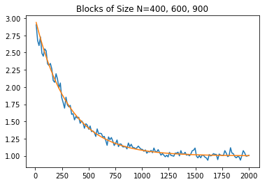
This is illustrated in figure 10.


V.4 A Trace Formula for Floquet Systems
The full hydrodynamic path integral with a time-dependent action (88) is highly complicated and non-universal. There are, however, still some statements we can make. For instance, we have a generalization of the trace formula in equation (15). We need to modify our definition of sectors so that they aren’t weakly coupled sectors of the Hamiltonian with the same energy, but weakly coupled sectors of the unitary with the same phase. For instance, in undriven systems we can consider states with energy separated by to be in different sectors, since they have the same phase and will not mix. Driving then allows mixing between sectors with energy differing by a multiple of . The SFF (with general Dyson index restored) is then
| (93) |
where is the transfer matrix connecting different sectors with the same quasi-energy . In the limit of an undriven Hamiltonian with no internal structure, is diagonal in energy. The trace then just counts how many energies correspond to a given quasienergy. When we integrate this factor over the range of quasienergies, we get the range of energies, as expected.
In another limit, after enough driving all states with energies differing by a multiple of will be fully mixed. The trace in Eq. (93) will then be unity, and the corresponding SFF is proportional to the number of periods up to a factor of the Dyson index,
| (94) |
The trace formula also generalizes equation (90) to general times given the explicit transition matrix .
Finally, note that the formula makes a sharp prediction at long times. If the range of energies in the unperturbed spectrum is , then we have a ramp coefficient per cycle of . Figure 11 is a graph illustrating this numerically.

VI Discussion
In this paper we developed a theory of the connected spectral form factor using tools from both RMT and hydrodynamics. This framework provides a number of key results, including formulas like equation (15) in cases with nearly conserved quantities, exemplified by equation (20). This allows us to rederive results previously only obtained for Floquet systems Friedman et al. 2019; Moudgalya et al. 2020 using general hydrodynamic principles. We are also able to give new formulas that include nonlinear effects as in equation (73). Such nonlinearities are typically associated with long-time tails in hydrodynamics Ernst et al. 1971Kovtun and Yaffe 2003 and here we see them manifest in the spectral form factor. Our results shed light on how spatial locality in Hamiltonians interacts with ergodicity. Finally, while we focused on the simplest case of energy diffusion for simplicity, analogous results can be obtained in a wide variety of hydrodynamic theories. Quite generally, the Thouless time can be read off from the decay rates of the slowest hydrodynamic modes. And in a system without slow modes, the Thouless time should scale like the logarithm of the system size, since any mode with a system-size-independent decay rate will have a system size suppressed amplitude after logarithmic time.
One emerging lesson highlighted by our work is that quantum chaos should be viewed as a robust property of a (dynamical) phase of matter. In particular, the emergence of a pure random matrix ramp after the Thouless time is a feature that is stable to small perturbations. In fact, as we emphasized, the linear growth with time as well as the exact coefficient of the ramp are seemingly universal. What evidence is there for this? First, when considering deformations , the derivative of the SFF with respect to is an expectation of an -type variable and such expectations are suppressed by factors of . This means the SFF is unaffected up to exponentially small corrections. Second, the addition of an ETH-obeying perturbation to the Hamiltonian corresponds to a stretching of the spectrum plus the addition of a random matrix. Hence, if the system had a linear ramp without this perturbation, it will also have one with the perturbation (see appendix D). Third, the basic phenomenon of the linear ramp comes from a symmetry breaking effect arising from the spontaneous breakdown of the relative time translation between the two SFF contours. Because this relative time translation symmetry cannot be explicitly broken by any time-independent Hamiltonian perturbation (i.e. without completely changing the problem), the corresponding symmetry broken phase should be both distinct from the unbroken phase and stable.
When we glimpse different manifestations of quantum chaos like hydrodynamics and ETH connecting to the emergence of RMT, it suggests to us that a larger synthesis may be possible. Certainly there are many connections between chaos, random matrix statistics, and eigenstate thermalization, e.g. as reviewed in D’Alessio et al. 2016, as well as connections to notions of complexity, e.g. Roberts and Yoshida 2017. However, work remains to understand how all the different timescales obtained from various manifestations of chaos fit together, e.g. Dymarsky 2018. We hope to elaborate on these points in future work.
There are several issues that are still not fully understood, leaving room for further work. One is whether hydrodynamic methods can derive plateau behaviors in SFFs. Such a path integral derivation would need be be very unusual to reproduce the fact that plateau behavior is non-perturbative in the Heisenberg time, . Perhaps inspiration could be taken from other path-integral derivations of plateaus such as Saad 2019; Altland and Sonner 2020; Müller et al. 2005. Another question is the role of disorder. It seems that hydrodynamic SFFs naturally spit out values consistent with disorder averaging, despite there being no explicit disorder-averaging in the definition of the CTP formulation. Certainly for non-periodic times, the CTP formulation does not require disorder averaging to get correct real-time dynamics Blake et al. 2018; Glorioso and Liu 2018. We need some disorder in order to make sense of the CTP action on the SFF contours, but this disorder can be small when the system size is large so that no intensive quantities, like transport parameters, are modified.
Finally, it is important to fully understand the possible effects of interactions in our modified CTP formalism. In the conventional CTP context, power counting indicates that interactions are irrelevant in the renormalization group sense. Interactions do generate novel effects not present in the Gaussian fixed point theory, but these effects can be captured in perturbation theory. The possibility of genuinely non-perturbative effects is not currently well understood. We showed that there are new effects arising from time periodicity, and carried out a partial resummation of diagrams to explore such effects. We found that they are subleading to the dominant quadratic behavior. However, it would be interesting to formulate a generalized renormalization group analysis to better understand the situation.
VII Acknowledgements
We thank Subhayan Sahu and Christopher White for helpful discussions throughout this process. This work is supported in part by the Simons Foundation via the It From Qubit Collaboration (B. S.) and by the Air Force Office of Scientific Research under award number FA9550-17-1-0180 (M.W.). M.W. is also supported by the Joint Quantum Institute.
Appendix A Appendix: Review of the SSS Wormhole Solution
In Saad et al. 2019 the authors (SSS) evaluate the ramp contribution exactly for the SYK model (see Appendix B). They start by noting that the SFF is a partition function on two contours. In particular, if we denote the collective fields of a single copy of the system by , the SFF is given by a path integral on two copies of the system with periodic time coordinates,
| (95) |
The essential insight in their paper is that for systems with many degrees of freedom, like the SYK model at large , this path integral can be evaluated by saddle-point methods and that a non-trivial family of saddle points give the ramp. These are thermofield double solutions at inverse temperature , suitably adjusted using images to account for the different boundary conditions, that correlate the two contours. At large such solutions always approximately solve the SFF two contour equations of motion because they solve the equations of motion on a contour (where the time evolutions trivially cancel) and the contours are identical in the ‘bulk’ of the forward and backward legs. Implicitly, we are appealing to the forgetfulness of chaotic systems, which here means that the solutions are exponentially insensitive to the boundary conditions.
Appendix B Appendix: Review of The SYK Model
The Sachdev-Ye-Kitaev (SYK) model is a disordered 0+1d system made of Majorana fermions with -body interactions ( is even) Sachdev and Ye 1993; Kitaev 2015; Polchinski and Rosenhaus 2016; Maldacena and Stanford 2016. The SYK Hamiltonian is given by
| (96) |
where represents the Majorana fermions and satisfy the anticommutation relation , and each is a Gaussian variable with mean zero and variance .
It is often convenient to perform a series of exact manipulations on Hamiltonian (96) to get a mean-field Lagrangian description of the SYK model in terms of bilocal variables consisting of a Green’s function and self-energy . In particular, one can write an expression for the imaginary temperature partition function of the SYK Model as
| (97) |
The SFF can be thought of as a partition function of a doubled system living on two contours, with one contour running forward in time (corresponding to in the SFF) and one contour running backward in time (corresponding to in the SFF). Generalizing the result for , one can write the SFF as
| (98) |
where a hat above a variable signals a matrix representation, . Because of the antiperiodic boundary conditions on the fermions, both and are antiperiodic under time shifts by . Note also that the measures and each integrate over the space of two-index functions of two variables.
Appendix C Appendix: CTP Formulation of Hydrodynamics
The Closed Time Path (CTP) formalism Glorioso and Liu 2018; Crossley et al. 2017 is an effective theory of hydrodynamics on the Schwinger-Keldysh contour. In Chen-Lin et al. 2019 a simplified version describing just energy diffusion is used to derive long-time-tails for two-point functions in hydrodynamics. We will largely follow their conventions. One starts with a partition function
| (99) |
where can be thought of as an external gauge field coupling to the conserved currents.
We express as , where is a nonlocal action. The main assumption is that after ‘integrating in’ slow modes the action will become local. In a standard hydrodynamic system, the only slow modes correspond to conservation laws and these modes are brought in to enforce those laws. We have
| (100) |
Where is a (generally complex) action functional.
As equation (100) makes manifest, the action doesn’t depend on the s except through the modified gauge fields . If we change variables to
| (101) |
we can derive additional identities. For instance unitary implies that
| (102) |
will always be zero whenever . In other words, if the chronologically latest insertion is -type, the expectation value is zero. This theorem is called the last time theorem, and is explored in detail in Gao et al. 2018. This, in turn, can be used to derive the fact that all terms in have at least one factor of an field. It is also worth explicitly noting the implications of the last time theorem for two point functions. We also always have
| (103) |
Additional constraints on CTP Lagrangians derived in other works include the fact all factors of the variables come with at least one time derivative and the KMS condition that .
It is also worth noting that we can formulate in terms of slightly different variables, replacing with the energy density . For the theory in Chen-Lin et al. 2019 used in the main text, at the Gaussian level is equal to plus higher derivative corrections. The general formula for is obtained by differentiating the action with respect to , since it couples to . For one conserved quantity at leading order in derivatives, the most general quadratic Lagrangian consistent with the requirements of derivatives and KMS symmetry is
| (104) |
To make the physics more transparent, it is useful to introduce an auxiliary variable . We can rewrite our action as
| (105) |
The action is now linear in , meaning that serves as a Lagrange multiplier enforcing the stochastic partial differential equation
| (106) |
where is now interpreted as a fluctuating force. This then leads to the probability distribution of energy modes discussed in the main text.
Appendix D Appendix: Folded Spectra
Here we comment on the case of stretched and folded spectra. To start with, consider a random Hamiltonian , where is a random matrix chosen from distribution (1) and is a smooth function with everywhere positive derivative. The quantum mechanics of such deformations have been considered recently in Gross et al. 2020. Another motivation to study folded spectra comes from the eigenstate thermalization hypothesis (ETH). ETH asserts that any local observable can be written as a sum of a smooth function of energy (related to the microcanonical expectation value) and a random-like erratic part Srednicki 1994; Deutsch 1991. Under this hypothesis, the SFF of a Hamiltonian perturbed by a local operator is then equivalent to the SFF of a stretched spectrum plus a random matrix, .
Studies of the SFFs of folded systems are common Gharibyan et al. 2018; Gubin and F. Santos 2012; Vahedi et al. 2016; Kudo 2005. One reason is that a folding procedure (often called ‘unfolding’) can be used to get semicircle statistics out of other level distributions in order to more easily compare numerical results with RMT. In this section we show analytically that non-singular folds indeed leave ramps invariant. For a comparison of folding versus filters as a way to look at parts of the spectrum see Nosaka et al. 2018.
Returning to , there is generically no such that is distributed according to (1). Rather, the pdf for is given by
| (107) |
Nonetheless, the spectral statistics of are very similar to those given by (1). This is because nearby eigenvalues still repel with repulsion term which is roughly proportional to . As such, the ramp still exists with coefficient given by (5).
Another way to see this is to consider a Gaussian filter function. If the variance in the filter function is small compared to the scale of variation in 22 2 For example, if is a slowly varying function of the energy density., then for the small window around , the stretching simply rescales all the differences between eigenvalues by , which is a trivial change. The effect on SFFs with broader filter functions can be obtained by integrating over .
Figure 12 shows coefficient plots of 5000 by 5000 GUE matrices after transformations and , accompanied by histograms of their spectral density
 |
 |
 |
 |
The next natural is question to ask is what happens when we choose a function which doubles back on itself, for instance . In these cases we can have multiple ‘species’ of eigenvalues near , corresponding to which branch of the original lies on. There is almost no repulsion between different species of eigenvalue, so the ramp part of the SFF is given by
| (108) |
 |
 |
 |
 |
One question that remains open is what the behavior is like near the turning points, characterized by , where the repulsion term becomes singular. Might there be a strong enough contribution to change the overall behavior?
References
- Haake (2010) F. Haake, Quantum Signatures of Chaos, Springer Series in Synergetics (Springer Berlin Heidelberg, 2010).
- Bohigas et al. (1984) O. Bohigas, M. J. Giannoni, and C. Schmit, “Characterization of chaotic quantum spectra and universality of level fluctuation laws,” Phys. Rev. Lett. 52, 1–4 (1984).
- Mehta (2004) M.L. Mehta, Random Matrices, ISSN (Elsevier Science, 2004).
- Dyson (1962) Freeman J. Dyson, “Statistical theory of the energy levels of complex systems. iii,” Journal of Mathematical Physics 3, 166–175 (1962), https://doi.org/10.1063/1.1703775 .
- Wigner and Griffin (1959) E.P. Wigner and J.J. Griffin, Group Theory and Its Application to the Quantum Mechanics of Atomic Spectra, Pure and applied Physics (Academic Press, 1959).
- Bohigas and Giannoni (1984) Oriol Bohigas and Marie-Joya Giannoni, “Chaotic motion and random matrix theories,” in Mathematical and computational methods in nuclear physics (Springer, 1984) pp. 1–99.
- Dubertrand and Müller (2016) Rémy Dubertrand and Sebastian Müller, “Spectral statistics of chaotic many-body systems,” New Journal of Physics 18, 033009 (2016).
- Bertini et al. (2018) Bruno Bertini, Pavel Kos, and Toma ž Prosen, “Exact spectral form factor in a minimal model of many-body quantum chaos,” Phys. Rev. Lett. 121, 264101 (2018).
- Cotler et al. (2017) Jordan S. Cotler, Guy Gur-Ari, Masanori Hanada, Joseph Polchinski, Phil Saad, Stephen H. Shenker, Douglas Stanford, Alexandre Streicher, and Masaki Tezuka, “Black holes and random matrices,” Journal of High Energy Physics 2017 (2017), 10.1007/jhep05(2017)118.
- Saad et al. (2019) Phil Saad, Stephen H. Shenker, and Douglas Stanford, “A semiclassical ramp in syk and in gravity,” (2019), arXiv:1806.06840 [hep-th] .
- Dubovsky et al. (2012) Sergei Dubovsky, Lam Hui, Alberto Nicolis, and Dam Thanh Son, “Effective field theory for hydrodynamics: Thermodynamics, and the derivative expansion,” Physical Review D 85 (2012), 10.1103/physrevd.85.085029.
- Grozdanov and Polonyi (2015a) Sa šo Grozdanov and Janos Polonyi, “Viscosity and dissipative hydrodynamics from effective field theory,” Phys. Rev. D 91, 105031 (2015a).
- Haehl et al. (2018) Felix M. Haehl, R. Loganayagam, and Mukund Rangamani, “Effective action for relativistic hydrodynamics: fluctuations, dissipation, and entropy inflow,” Journal of High Energy Physics 2018 (2018), 10.1007/jhep10(2018)194.
- Crossley et al. (2017) Michael Crossley, Paolo Glorioso, and Hong Liu, “Effective field theory of dissipative fluids,” (2017), arXiv:1511.03646 [hep-th] .
- Jensen et al. (2018) Kristan Jensen, Natalia Pinzani-Fokeeva, and Amos Yarom, “Dissipative hydrodynamics in superspace,” Journal of High Energy Physics 2018 (2018), 10.1007/jhep09(2018)127.
- Altshuler and Shklovskii (1986) O. L. Altshuler and B. I. Shklovskii, “Repulsion of energy levels and conductivity of small metal samples,” JETP 64, 127 (1986).
- Schiulaz et al. (2019) Mauro Schiulaz, E. Jonathan Torres-Herrera, and Lea F. Santos, “Thouless and relaxation time scales in many-body quantum systems,” Physical Review B 99 (2019), 10.1103/physrevb.99.174313.
- Gharibyan et al. (2018) Hrant Gharibyan, Masanori Hanada, Stephen H. Shenker, and Masaki Tezuka, “Onset of random matrix behavior in scrambling systems,” Journal of High Energy Physics 2018 (2018), 10.1007/jhep07(2018)124.
- Friedman et al. (2019) Aaron J. Friedman, Amos Chan, Andrea De Luca, and J. T. Chalker, “Spectral statistics and many-body quantum chaos with conserved charge,” Physical Review Letters 123 (2019), 10.1103/physrevlett.123.210603.
- Altland and Bagrets (2018) Alexander Altland and Dmitry Bagrets, “Quantum ergodicity in the syk model,” Nuclear Physics B 930, 45–68 (2018).
- Nosaka et al. (2018) Tomoki Nosaka, Dario Rosa, and Junggi Yoon, “The thouless time for mass-deformed syk,” Journal of High Energy Physics 2018 (2018), 10.1007/jhep09(2018)041.
- García-García and Verbaarschot (2017) Antonio M. García-García and Jacobus J. M. Verbaarschot, “Analytical spectral density of the sachdev-ye-kitaev model at finite n,” Physical Review D 96 (2017), 10.1103/physrevd.96.066012.
- Altland and Sonner (2020) Alexander Altland and Julian Sonner, “Late time physics of holographic quantum chaos,” (2020), arXiv:2008.02271 [hep-th] .
- Roy and Prosen (2020) Dibyendu Roy and Tomaž Prosen, “Random matrix spectral form factor in kicked interacting fermionic chains,” Physical Review E 102 (2020), 10.1103/physreve.102.060202.
- D’Alessio et al. (2016) Luca D’Alessio, Yariv Kafri, Anatoli Polkovnikov, and Marcos Rigol, “From quantum chaos and eigenstate thermalization to statistical mechanics and thermodynamics,” Advances in Physics 65, 239–362 (2016).
- Heusler et al. (2004) Stefan Heusler, Sebastian Müller, Petr Braun, and Fritz Haake, “Universal spectral form factor for chaotic dynamics,” Journal of Physics A: Mathematical and General 37, L31 (2004).
- Brézin and Hikami (1997) E Brézin and S Hikami, “Spectral form factor in a random matrix theory,” Physical Review E 55, 4067 (1997).
- Kovtun (2012) Pavel Kovtun, “Lectures on hydrodynamic fluctuations in relativistic theories,” Journal of Physics A: Mathematical and Theoretical 45, 473001 (2012).
- Grozdanov and Polonyi (2015b) Sašo Grozdanov and Janos Polonyi, “Viscosity and dissipative hydrodynamics from effective field theory,” Physical Review D 91 (2015b), 10.1103/physrevd.91.105031.
- Endlich et al. (2013) Solomon Endlich, Alberto Nicolis, Rafael A. Porto, and Junpu Wang, “Dissipation in the effective field theory for hydrodynamics: First-order effects,” Physical Review D 88 (2013), 10.1103/physrevd.88.105001.
- Glorioso and Liu (2018) Paolo Glorioso and Hong Liu, “Lectures on non-equilibrium effective field theories and fluctuating hydrodynamics,” (2018), arXiv:1805.09331 [hep-th] .
- Haehl et al. (2017) Felix M. Haehl, R. Loganayagam, and Mukund Rangamani, “Schwinger-keldysh formalism. part i: Brst symmetries and superspace,” Journal of High Energy Physics 2017 (2017), 10.1007/jhep06(2017)069.
- Kamenev and Levchenko (2009) Alex Kamenev and Alex Levchenko, “Keldysh technique and non-linear sigma-model: basic principles and applications,” Advances in Physics 58, 197–319 (2009).
- chao Chou et al. (1985) Kuang chao Chou, Zhao bin Su, Bai lin Hao, and Lu Yu, “Equilibrium and nonequilibrium formalisms made unified,” Physics Reports 118, 1 – 131 (1985).
- Gromov et al. (2020) Andrey Gromov, Andrew Lucas, and Rahul M. Nandkishore, “Fracton hydrodynamics,” Physical Review Research 2 (2020), 10.1103/physrevresearch.2.033124.
- Nandkishore and Hermele (2019) Rahul M. Nandkishore and Michael Hermele, “Fractons,” Annual Review of Condensed Matter Physics 10, 295–313 (2019).
- Moudgalya et al. (2020) Sanjay Moudgalya, Abhinav Prem, David A. Huse, and Amos Chan, “Spectral statistics in constrained many-body quantum chaotic systems,” (2020), arXiv:2009.11863 [cond-mat.stat-mech] .
- Chen-Lin et al. (2019) Xinyi Chen-Lin, Luca V. Delacrétaz, and Sean A. Hartnoll, “Theory of diffusive fluctuations,” Physical Review Letters 122 (2019), 10.1103/physrevlett.122.091602.
- Sachdev and Ye (1993) Subir Sachdev and Jinwu Ye, “Gapless spin-fluid ground state in a random quantum heisenberg magnet,” Physical Review Letters 70, 3339–3342 (1993).
- Kitaev (2015) A Kitaev, “A simple model of quantum holography,” in KITP Progr. Entanglement Strongly-Correlated Quantum Matter (2015).
- Polchinski and Rosenhaus (2016) Joseph Polchinski and Vladimir Rosenhaus, “The spectrum in the sachdev-ye-kitaev model,” Journal of High Energy Physics 2016, 1–25 (2016).
- Maldacena and Stanford (2016) Juan Maldacena and Douglas Stanford, “Remarks on the sachdev-ye-kitaev model,” Physical Review D 94 (2016), 10.1103/physrevd.94.106002.
- Ernst et al. (1971) M. H. Ernst, E. H. Hauge, and J. M. J. van Leeuwen, “Asymptotic time behavior of correlation functions. i. kinetic terms,” Phys. Rev. A 4, 2055–2065 (1971).
- Kovtun and Yaffe (2003) Pavel Kovtun and Laurence G. Yaffe, “Hydrodynamic fluctuations, long-time tails, and supersymmetry,” Physical Review D 68 (2003), 10.1103/physrevd.68.025007.
- Roberts and Yoshida (2017) Daniel A. Roberts and Beni Yoshida, “Chaos and complexity by design,” Journal of High Energy Physics 2017 (2017), 10.1007/jhep04(2017)121.
- Dymarsky (2018) Anatoly Dymarsky, “Bound on eigenstate thermalization from transport,” (2018), arXiv:1804.08626 [cond-mat.stat-mech] .
- Saad (2019) Phil Saad, “Late time correlation functions, baby universes, and eth in jt gravity,” (2019), arXiv:1910.10311 [hep-th] .
- Müller et al. (2005) Sebastian Müller, Stefan Heusler, Petr Braun, Fritz Haake, and Alexander Altland, “Periodic-orbit theory of universality in quantum chaos,” Physical Review E 72 (2005), 10.1103/physreve.72.046207.
- Blake et al. (2018) Mike Blake, Hyunseok Lee, and Hong Liu, “A quantum hydrodynamical description for scrambling and many-body chaos,” Journal of High Energy Physics 2018 (2018), 10.1007/jhep10(2018)127.
- Gao et al. (2018) Ping Gao, Paolo Glorioso, and Hong Liu, “Ghostbusters: Unitarity and causality of non-equilibrium effective field theories,” (2018), arXiv:1803.10778 [hep-th] .
- Gross et al. (2020) David J. Gross, Jorrit Kruthoff, Andrew Rolph, and Edgar Shaghoulian, “Hamiltonian deformations in quantum mechanics, tt¯ , and the syk model,” Physical Review D 102 (2020), 10.1103/physrevd.102.046019.
- Srednicki (1994) Mark Srednicki, “Chaos and quantum thermalization,” Phys. Rev. E 50, 888–901 (1994).
- Deutsch (1991) J. M. Deutsch, “Quantum statistical mechanics in a closed system,” Phys. Rev. A 43, 2046–2049 (1991).
- Gubin and F. Santos (2012) Aviva Gubin and Lea F. Santos, “Quantum chaos: An introduction via chains of interacting spins 1/2,” American Journal of Physics 80, 246–251 (2012).
- Vahedi et al. (2016) J. Vahedi, A. Ashouri, and S. Mahdavifar, “Quantum chaos in the heisenberg spin chain: The effect of dzyaloshinskii-moriya interaction,” Chaos: An Interdisciplinary Journal of Nonlinear Science 26, 103106 (2016).
- Kudo (2005) Kazue Kudo, Statistical and Dynamical Properties in the Energy Spectra of XXZ Spin Chains, Ph.D. thesis (2005).