A model for dynamical solvent control of molecular junction electronic properties

Maxim F. Gelin Note: E-mail: maxim@hdu.edu.cn Affiliation: School of Sciences, Hangzhou Dianzi University, 310018 Hangzhou, China Daniel S. Kosov Note: E-mail: daniel.kosov@jcu.edu.au Affiliation: College of Science and Engineering, James Cook University, Townsville, QLD, 4811, Australia

Abstract

Experimental measurements of electron transport properties of molecular junctions are often performed in solvents. Solvent-molecule coupling and physical properties of the solvent can be used as the external stimulus to control electric current through a molecule. In this paper, we propose a model, which includes dynamical effects of solvent-molecule interaction in the non-equilibrium Green’s function calculations of electric current. The solvent is considered as a macroscopic dipole moment that reorients stochastically and interacts with the electrons tunnelling through the molecular junction. The Keldysh-Kadanoff-Baym equations for electronic Green’s functions are solved in time-domain with subsequent averaging over random realisations of rotational variables using Furutsu-Novikov method for exact closure of infinite hierarchy of stochastic correlation functions. The developed theory requires the use of wide-band approximation as well as classical treatment of solvent degrees of freedom. The theory is applied to a model molecular junction. It is demonstrated that not only electrostatic interaction between molecular junction and solvent but also solvent viscosity can be used to control electrical properties of the junction. Aligning of the rotating dipole moment breaks particle-hole symmetry of the transmission favouring either hole or electron transport channels depending upon the aligning potential.

I Introduction

The single-molecule electrical experiments now go way beyond the initial current as a function of applied voltage measurements. The environment is no longer playing a passive role but used as experimental means to control electronic properties of molecular electronic junction.Xiang et al. 2016 Mechanical stretching, $\pi$ stacking,Wu et al. 2008 hydrogen bondingNishino et al. 2013 and supramolecular interactions Bui et al. 2013 have been used to change electrical properties of molecular junctions. Recently, there is a growing interest in the use of solvent to control transport of electrons in single-molecule junction. Kuznetsov 2007; Milan et al. 2016; Dzhioev and Kosov 2012; Leary et al. 2009; Stipe et al. 1997; Luka-Guth et al. 2016; Kotiuga et al. 2015; Fatemi et al. 2011; Ghane et al. 2015; Kuznetsov 2007; Choi et al. 2016; Kornyshev et al. 2006

The scope of theoretical studies of solvated molecular electronic junctions is somewhat limited. On the computational side, density functional theory nonequilibrium Green’s function based calculations take into account a few surrounding solvent molecules kept in the fixed optimised geometry to mimic the effect of molecule-solvent interaction.Leary et al. 2009; Milan et al. 2016; Ghane et al. 2015 Several simple models were developed to treat electrolyte environment of molecular electronic junctions via Poisson-Boltzmann equations incorporating effect of the solvent into voltage drop across the junction with subsequent rate equation calculations of electric current.Kornyshev et al. 2006; Zhang et al. 2008 Born solvation model was combined in the self-consistent manner with static nonequilibrium Green’s functions calculations electric current calculations to treat the problem.Luka-Guth et al. 2016

These theoretical works provide an important insight on the role of the solvent, however, they all assumed that the time-scales for electrons and solvent motion can be completely separated. In other words, all time-dependent effects from solvent response and rearrangement due to the dynamical charging and discharging of the molecular junction by current-carrying electrons have been neglected. In this paper, we developed the model which takes into account solvent dynamics. The solvent is modelled as a macroscopic, stochastically rotating dipole moment which interacts with the electrons tunnelling through the molecular junction. This interaction makes the Hamiltonian for quantum transport problem explicitly time-dependent which is handled exactly by nonequilibrium Green’s functions calculations. The evaluation of observables obtained from electronic Green’s functions requires the averaging over realisations of Gaussian stochastic process, which is performed using Furutsu-Novikov method for stochastic calculus.Klyatskin 2005 As far as time-evolution of the system is concerned, quantum electronic dynamics are treated on an equal footing with classical solvent dynamics in our method.

The paper is organised as follows. Section II describes the theory. It introduces model Hamiltonian for molecular junctions, main definitions for Green’s functions and self-energies, as well as describes solution of the Keldysh-Kadanoff-Baym equations coupled to the stochastic rotor dynamics. Section II also provides expression for electronic current averaged over stochastic realisations of solvent dynamics and details the use of Furutsu-Novikov method. Section III illustrates the theory by calculations on model molecular systems and discusses the main physical observations. The main results of the paper are summarised in section IV. The technical details of the derivations and numerical algorithm description are relegated to the appendices.

II Theory

II.1 Model Hamiltonian

In this section we discuss the physical model for molecular electronic junction coupled to solvent. The system Hamiltonian consists of five parts

H(t)=H_{\text{molecule}}+H_{\text{leads}}+H_{\text{solvent}}(t)\\ +H_{\text{leads-molecule}}+H_{\text{solvent-molecule}}(t).

(1)

Here $H_{\text{molecule}}$ is the molecular Hamiltonian, $H_{\text{leads}}$ describes electron reservoirs in the right and left leads. Coupling between the molecule and the leads is given by $H_{\text{leads-molecule}}$ . The solvent is described by $H_{\text{solvent}}$ and the coupling between molecule and the solvent is denoted by $H_{\text{solvent-molecule}}$ , these parts of the Hamiltonian are time-dependent.

The molecule is modelled as a single resonant-level, which can be occupied by the zero or one spin-less electrons (the electron spin will not be considered explicitly in our derivations but we will recreate the factor of two due to spin degeneracy in the final expressions for electric current). The corresponding Hamiltonian is

H_{\text{molecule}}=\epsilon d^{\dagger}d,

(2)

where $d^{\dagger}$ ( $d$ ) creates (annihilates) electron on molecular orbital with energy $\epsilon$ .

The left and right leads are modelled as macroscopic reservoirs of non-interacting electrons

H_{\text{leads}}=\sum_{k\alpha}\epsilon_{k\alpha}d^{\dagger}_{k\alpha}d_{k\alpha},

(3)

where $d^{\dagger}_{k\alpha}$ and $d_{k\alpha}$ are the creation and annihilation operators for a single particle state of energies $\epsilon_{k\alpha}$ for left $\alpha=L$ or right $\alpha=R$ leads. The couplings between leads and molecule are described by the tunnelling interaction

H_{\text{leads-molecule}}=\sum_{k\alpha}(t_{k\alpha}d^{\dagger}_{k\alpha}d+t^{*}_{k\alpha}d^{\dagger}d_{k\alpha}),

(4)

where $t_{k\alpha}$ is the tunnelling amplitude between molecule and leads states.

The solvent, which is modelled as classical rigid rotating dipole moment $\mathbf{\mu}$ with moment of inertia $I$ , is described by the time-dependent Hamiltonian

H_{\text{solvent}}(t)=\frac{1}{2I}\left(\frac{d\phi}{dt}\right)^{2},

(5)

where $\phi$ is the orientation angle of the dipole moment relative to the molecule. This level of description of solute-solvent interactions is common in theory of rotational relaxation in polar solvents and constitutes the essence of stochastic cage model Coffey et al. 1996, where the solvent shell surrounding the molecule is described as an effective quasiparticle which interacts with the molecule by appropriate anisotropic potential and stochastically interacts with the balk solvent. We thus assume that the orientation angle $\phi$ and the conjugated rotational frequency $\Omega$ obey the stochastic evolution equations

\frac{d\phi(t)}{dt}=\Omega(t),

(6)

and

\frac{d\Omega(t)}{dt}=G(\phi(t))-\xi\Omega(t)+F(t).

(7)

Here $U(\phi)$ is an external potential,

G(\phi)=-\frac{dU(\phi)}{d\phi}

(8)

is the torque acting on the rotator, and $F(t)$ is a $\delta$ -correlated stochastic Gaussian process,

\langle F(t)\rangle=0,\,\,\,\langle F(t)F(t^{\prime})\rangle=2\xi\delta(t-t^{\prime}),

(9)

where $\xi$ is the rotational friction. The fluctuation-dissipation theorem relation between the noise and viscosity is assumed here, which implies that the solvent is maintained in thermodynamic equilibrium. We use the dimensionless variables, in which $\Omega$ and $\xi$ are expressed in units of $\sqrt{k_{B}T/I}$ , where $k_{B}$ is Boltzmann’s constant and $T$ is a temperature.

The interaction between the molecule and the solvent is given by point charge-dipole interaction

H_{\text{solvent-molecule}}(t)=\frac{1}{4\pi\epsilon_{0}}\frac{ed^{\dagger}d\;\mu\cos(\phi)}{r^{2}},

(10)

where the instantaneous charge of the molecule due to tunnelling of electrons is given by electron number operator $d^{\dagger}d$ multiplied by electron charge $e$ , $\mu$ is magnitude of the classical dipole moment and $r$ is the distance between molecule and solvent cage centre of mass, and $\epsilon_{0}$ is electrical permittivity. As typical in electron transport calculation we assume that $e$ carries the negative sign ( $e=-|e|$ ). This part of the Hamiltonian is explicitly time-dependent due to angle $\phi$ being time-dependent variable undergoing stochastic fluctuations. Of course, such a treatment of solvent-molecule interaction is an oversimplification, but it allows us to conveniently rewrite Eq. (10) as

H_{\text{solvent-molecule}}(t)=-\lambda\cos(\phi),

(11)

where the parameter

\lambda=-\frac{1}{4\pi\epsilon_{0}}\frac{e\mu}{r^{2}}.

(12)

can be interpreted as an effective solvent-molecule coupling strength. Eqs. (5)-(11) describe a variant of the stochastic cage model which is called the itinerant oscillator model Coffey et al. 1996. Despite its simplicity, this model captures essential physics. It was successfully applied to the description of molecular rotation in polar liquids and solvents.

It is convenient to include solvent-molecule interaction into the molecule Hamiltonian by introducing time-dependent energy level

h(\phi(t))=\epsilon-\lambda\text{cos}(\phi(t)).

(13)

Then combining two terms together we get

H_{\text{molecule}}+H_{\text{solvent-molecule}}=h(\phi(t))d^{\dagger}d.

(14)

II.2 Green’s functions and self-energies

In this section, Green’s functions and self-energies definitions are introduced and basic notation is established; they will be used throughout the paper. The exact and non-adiabatic (computed along a given angular trajectory $\phi(t)$ ) retarded, advanced and lesser Green’s functions in the molecular space are defined as Haug and Jauho 2010

\mathcal{G}^{R}(t,t^{\prime})=-i\theta(t-t^{\prime})\langle\{d(t),d^{\dagger}(t^{\prime})\}\rangle,

(15)

\mathcal{G}^{A}(t,t^{\prime})=\Big({\cal G}^{R}(t^{\prime},t)\Big)^{*}

(16)

and

\mathcal{G}^{<}(t,t^{\prime})=i\langle d^{\dagger}(t^{\prime})d(t)\rangle.

(17)

The retarded, advanced and lesser self-energies for $\alpha$ lead are given by the standard expressions

{\Sigma}_{\alpha}^{R}(t,t^{\prime})=-i{{}\theta(t-t^{\prime})}\sum_{k}t^{*}_{k\alpha}e^{-i\epsilon_{k}(t-t^{\prime})}t_{k\alpha},

(18)

{\Sigma}_{\alpha}^{A}(t,t^{\prime})=\Big({\Sigma}_{\alpha}^{R}(t^{\prime},t)\Big)^{*},

(19)

{\Sigma}_{\alpha}^{<}(t,t^{\prime})=2\pi i\sum_{k}t^{*}_{k\alpha}f_{\alpha}(\epsilon_{k})e^{-i\epsilon_{k}(t-t^{\prime})}t_{k\alpha}.

(20)

Here $f_{\alpha}$ is the Fermi-Dirac distribution. The total self-energies are the sum of contributions from the left and right leads as

{\Sigma}^{R,A,<}(t,t^{\prime})={\Sigma}^{R,A,<}_{L}(t,t^{\prime})+{\Sigma}_{R}^{R,A,<}(t,t^{\prime}).

(21)

The self-energies in energy-domain are defined as a Fourier transformation

{\Sigma}^{R,A,<}(\omega)=\int d(t-t^{\prime})e^{i\omega(t-t^{\prime})}{\Sigma}^{R,A,<}(t,t^{\prime}).

(22)

The wide-band approximation will be used in our derivations and calculations: within this approximation the time-dependence of retarded and advanced self-energies is reduced to delta-function

\Sigma_{\alpha}^{R}(t,t^{\prime})=-\frac{i}{2}\Gamma_{\alpha}\delta(t-t^{\prime}),\;\;\;\Sigma_{\alpha}^{A}(t,t^{\prime})=\frac{i}{2}\Gamma_{\alpha}\delta(t-t^{\prime}),

(23)

where the level-broadening function $\Gamma_{\alpha}$ is time-independent parameter which describes the strength of molecule-lead coupling. The wide-band approximation means the assumption that both the leads’ density of states and all tunneling amplitudes between leads’ and molecular states are energy-independent constants. Our approach depends critically on the use of the wind-band approximation to solve analytically Keldysh-Kadanoff-Baym equations.

Notice that we set $\hbar=1$ in all definitions of Green’s functions. This implies that all quantum mechanical energy related quantities $\epsilon$ , $\lambda$ , and $\Gamma_{\alpha}$ are scaled by $\hbar$ and measured in the units of frequency (1/time).

II.3 Solution of Keldysh-Kadanoff-Baym equations and expression for the current

Suppose that a stochastic trajectory of the dipole rotation angle $\phi(t)$ is known from the solution of the Langevin equation. Our goal in this section is to solve exactly Keldysh-Kadanoff-Baym equations for the Green’s functions and consequently obtain a concise expression for electric current averaged over the stochastic trajectory $\phi(t)$ .

We begin with the general expression for electric current from $\alpha$ lead in time-dependent systemHaug and Jauho 2010

J_{\alpha}(t)=2e\text{ Re }\int_{-\infty}^{+\infty}dt^{\prime}\Big[\mathcal{G}^{<}(t,t^{\prime})\Sigma_{\alpha}^{A}(t^{\prime},t)\\ +\mathcal{G}^{R}(t,t^{\prime})\Sigma_{\alpha}^{<}(t^{\prime},t)\big].

(24)

Next, we transform self-energies to the energy domain whilst leaving molecular Green’s functions time-dependent

J_{\alpha}(t)=2e\text{ Re }\int_{-\infty}^{+\infty}\frac{d\omega}{2\pi}\int_{-\infty}^{+\infty}dt^{\prime}e^{-i\omega(t^{\prime}-t)}\\ \times\Big[\mathcal{G}^{<}(t,t^{\prime})\Sigma_{\alpha}^{A}(\omega)+\mathcal{G}^{R}(t,t^{\prime})\Sigma_{\alpha}^{<}(\omega)\big].

(25)

Electric current should satisfy the continuity equation at each time moment $t$

\frac{dN}{dt}=J_{L}(t)+J_{R}(t),

(26)

where $N$ is the total number of electrons in the molecule at time $t$ . Using the continuity equation and rearranging the terms, we eliminate lesser Green’s function from the expression and get

J_{L}(t)=\frac{\Gamma_{L}}{\Gamma}\Big\{\frac{dN}{dt}-2e\Gamma_{R}\text{ Im }\int_{-\infty}^{+\infty}\frac{d\omega}{2\pi}\int_{-\infty}^{+\infty}dt^{\prime}e^{-i\omega(t^{\prime}-t)}\mathcal{G}^{R}(t,t^{\prime})[f_{L}(\omega)-f_{R}(\omega)]\Big\}.

(27)

Let us average the above equation over the stochastic realisation of the dipole moment rotation process. The average

\langle\frac{dN}{dt}\rangle=0

(28)

obviously disappears, otherwise the molecule would either accumulate or loose charge continuously. The averaged current becomes

\langle J_{L}\rangle=-2e\frac{\Gamma_{L}\Gamma_{R}}{\Gamma}\\ \text{ Im }\int_{-\infty}^{+\infty}\frac{d\omega}{2\pi}\int_{-\infty}^{+\infty}dt^{\prime}e^{-i\omega(t^{\prime}-t)}\langle\mathcal{G}^{R}(t,t^{\prime})\rangle[f_{L}(\omega)-f_{R}(\omega)].

(29)

Notice, that the averaged electric current does not depend on time, since the retarded Green’s function will depend on relative time only once averaged over the stochastic realisations.

Our next goal is to find the explicit expression for the retarded Green’s function to enter it into the expression to electric current. We begin with the Keldysh-Kadanoff-Baym equation for the retarded Green’s functionHaug and Jauho 2010

(i\partial_{t}-h(t))\mathcal{G}^{R}(t,t^{\prime})\\ -\int_{-\infty}^{+\infty}dt_{1}\Sigma^{R}(t,t_{1})\mathcal{G}^{R}(t_{1},t^{\prime})=\delta(t-t^{\prime}).

(30)

It is reduced in the wide-band approximation to

(i\partial_{t}-h(t))\mathcal{G}^{R}(t,t^{\prime})-\frac{i}{2}\Gamma\mathcal{G}^{R}(t_{1},t^{\prime})=\delta(t-t^{\prime}),

(31)

where $h(t)$ denotes $h(\phi(t))$ given by equation (13) and

\Gamma=\Gamma_{L}+\Gamma_{R}

(32)

is the total level-broadening function. This differential equation can be solved analytically and yields

\mathcal{G}^{R}(t,t^{\prime})=-i{{}\theta(t-t^{\prime})}e^{-\frac{1}{2}\Gamma(t-t^{\prime})}e^{-i\int^{t}_{t^{\prime}}dt_{1}h(t_{1})}

(33)

Notice that analytical expression (33) requires the wide-band approximation treatment for leads’ self-energies. Substituting retarded Green’s function (33) into the expression for current (29) gives

\langle J_{L}\rangle=2e\frac{\Gamma_{L}\Gamma_{R}}{\Gamma}\text{ Re }\int_{-\infty}^{+\infty}\frac{d\omega}{2\pi}\int_{-\infty}^{t}dt^{\prime}e^{-i(\omega-\frac{i}{2}\Gamma)(t-t^{\prime})}\langle e^{-i\int^{t}_{t^{\prime}}dt_{1}h(t_{1})}\rangle[f_{L}(\omega)-f_{R}(\omega)].

(34)

Changing variables of integration to $\tau=t-t^{\prime}$ and taking into account that quantity $\langle e^{-i\int^{t}_{t^{\prime}}dt_{1}h(t_{1})}\rangle$ depends on relative time only once averaged over realisations of the stochastic process we arrive to

\langle J_{L}\rangle=2e\frac{\Gamma_{L}\Gamma_{R}}{\Gamma}\text{ Re }\int_{-\infty}^{+\infty}\frac{d\omega}{2\pi}\int^{\infty}_{0}d\tau e^{-i(\omega-\frac{i}{2}\Gamma)\tau)}R(\tau)[f_{L}(\omega)-f_{R}(\omega)]

(35)

where

R(\tau)=\langle e^{-i\int^{\tau}_{0}dt_{1}h(t_{1})}\rangle

(36)

Eq. (35) can be rewritten in the Landauer form

\langle J_{L}\rangle=e\int_{-\infty}^{+\infty}\frac{d\omega}{2\pi}T(\omega)[f_{L}(\omega)-f_{R}(\omega)]

(37)

where we have introduced ”transmission coefficient”

T(\omega)=2\frac{\Gamma_{L}\Gamma_{R}}{\Gamma}\text{ Re }\int^{\infty}_{0}d\tau e^{-i(\omega-\frac{i}{2}\Gamma)\tau)}R(\tau).

(38)

Notice that although being called ”transmission coefficient”, $T(\omega)$ given by (38) should not be assigned the meaning of probability for electron with energy $\omega$ to tunnel across the molecule, since the inelastic processes due to the dynamical coupling of tunnelling electron with rigid rotator are included into our consideration.

II.4 Averaging over the stochastic solvent dynamics

The aim here is to develop a method to compute $R(t)$ of Eq. (36) (for convenience of notation, $t$ will be used as a variable in $R(t)$ ) where averaging $\langle...\rangle$ is performed over realisations of stochastic variable $\phi$ and time-evolution of $\phi(t)$ is given by stochastic differential equations (6) and (7).

Let us define the quantity

A_{t}([\phi(\tau)])=e^{-i\int_{0}^{t}dt_{1}h(\phi(t_{1}))}.

(39)

Hereafter, the notation $A_{t}[\phi(\tau)]$ means that $A$ is a function of $t$ and a functional of the stochastic process $\phi(\tau)$ . Evidently,

R(t)=\langle A_{t}([\phi(\tau)])\rangle.

(40)

Let us now introduce the stochastic functional

R(\phi,\Omega,t)=\delta(\phi-\phi(t))\delta(\Omega-\Omega(t))A_{t}[\phi(\tau)]

(41)

where $\phi(t)$ and $\Omega(t)$ are certain realisations of the stochastic processes (6) and (7). Averaging Eq. (41) over all realisations of these processes yields

\rho(\phi,\Omega,t)=\left\langle R(\phi,\Omega,t)\right\rangle,

(42)

which can be interpreted as a probability density of $A_{t}[\phi(\tau)]$ to have a certain value given $\phi(t)$ and $\Omega(t)$ are equaled to $\phi$ and $\Omega$ at a time moment $t$ . Then, according to van Kampen lemma,Van Kampen 2007 we obtain

R(t)=\int_{-\infty}^{\infty}d\Omega\int_{0}^{2\pi}d\phi\rho(\phi,\Omega,t).

(43)

We are in the position now to derive a closed-form Fokker-Planck equation for $\rho(\phi,\Omega,t)$ . Formally differentiating $R(\phi,\Omega,t)$ with respect to time, using stochastic equations (6) and (7) and taking the average, we obtain

\partial_{t}\rho(\phi,\Omega,t)=\Big(-ih(\phi)-\Omega\partial_{\phi}-G(\phi)\partial_{\Omega}+\xi\partial_{\Omega}\Omega\Big)\rho(\phi,\Omega,t)\\ -\partial_{\Omega}\Omega\left\langle F(t)R(\phi,\Omega,t)\right\rangle.

(44)

Employing the Furutsu-Novikov formulaKlyatskin 2005, we get

\left\langle F(t)R(\phi,\Omega,t)\right\rangle=\intop_{0}^{t}dt^{\prime}\left\langle F(t)F(t^{\prime})\right\rangle\left\langle\frac{\delta R(\phi,\Omega,t)}{\delta F(t^{\prime})}\right\rangle.

(45)

To evaluate the functional derivative, we follow the method of Ref. Klyatskin 2005:

\frac{\delta R(\phi,\Omega,t)}{\delta F(t^{\prime})}=\Big(-\partial_{\phi}\frac{\delta\phi(t)}{\delta F(t^{\prime})}-\partial_{\Omega}\frac{\delta\Omega(t)}{\delta F(t^{\prime})}\\ -i\int_{0}^{t}dt^{\prime\prime}\frac{\delta h(\phi(t^{\prime\prime}))}{\delta F(t^{\prime})}\Big)\delta(\phi-\phi(t))\delta(\Omega-\Omega(t))A_{t}[\phi(\tau)]\\ =\Big(-\partial_{\phi}\frac{\delta\phi(t)}{\delta F(t^{\prime})}-\partial_{\Omega}\frac{\delta\Omega(t)}{\delta F(t^{\prime})}\\ +i\lambda\int_{0}^{t}dt^{\prime\prime}\sin(\phi(t^{\prime\prime}))\frac{\delta\phi(t^{\prime\prime})}{\delta F(t^{\prime})}\Big)\delta(\phi-\phi(t))\delta(\Omega-\Omega(t))A_{t}[\phi(\tau)].

(46)

The stochastic equations (6) and (7) can be rewritten in the integral form as follows:

\phi(t)=\phi(0)+\intop_{0}^{t}d\tau\int_{-\infty}^{\infty}d\Omega\Omega\delta(\Omega-\Omega(\tau)),

(47)

and

\Omega(t)=\Omega(0)+\intop_{0}^{t}d\tau\left(G(\phi(\tau))+\xi\Omega(\tau)+F(\tau)\right)=\\ \Omega(0)+\intop_{0}^{t}d\tau\int_{-\infty}^{\infty}d\Omega\int_{0}^{2\pi}d\phi\left(G(\phi)+\xi\Omega+F(\tau)\right)\delta(\phi-\phi(\tau))\delta(\Omega-\Omega(\tau)).

(48)

Differentiating (47) and (48) with respect to $F(t^{\prime})$ , we obtain:

\frac{\delta\phi(t)}{\delta F(t^{\prime})}=-\intop_{t^{\prime}}^{t}d\tau\int_{-\infty}^{\infty}d\Omega\Omega\partial_{\Omega}\delta(\Omega-\Omega(\tau))\frac{\delta\Omega(\tau)}{\delta F(t^{\prime})},

(49)

\frac{\delta\Omega(t)}{\delta F(t^{\prime})}=\intop_{0}^{t}d\tau\int_{-\infty}^{\infty}d\Omega\int_{0}^{2\pi}d\phi\left[\frac{\delta F(t)}{\delta F(t^{\prime})}-\left(G(\phi)+\xi\Omega+F(\tau)\right)\left(\partial_{\phi}\frac{\delta\phi(t)}{\delta F(t^{\prime})}+\partial_{\Omega}\frac{\delta\phi(t)}{\delta F(t^{\prime})}\right)\right]\delta(\phi-\phi(\tau))\delta(\Omega-\Omega(\tau))\\ =1-\intop_{t^{\prime}}^{t}d\tau\int_{-\infty}^{\infty}d\Omega\int_{0}^{2\pi}d\phi\left[\left(G(\phi)+\xi\Omega+F(\tau)\right)\left(\partial_{\phi}\frac{\delta\phi(t)}{\delta F(t^{\prime})}+\partial_{\Omega}\frac{\delta\phi(t)}{\delta F(t^{\prime})}\right)\right]\delta(\phi-\phi(\tau))\delta(\Omega-\Omega(\tau)).

(50)

Due to causality, we have replaced

\intop_{0}^{t}d\tau\rightarrow\intop_{t^{\prime}}^{t}d\tau

(51)

because

\frac{\delta\phi(t)}{\delta F(t^{\prime})}=\frac{\delta\Omega(t)}{\delta F(t^{\prime})}=0\,\,\,\mathrm{for}\,\,\tau<t^{\prime}.

(52)

Since the stochastic torque $F(t)$ is delta-correlated (Eq. (9)), we need to evaluate the functional derivative at $t^{\prime}=t.$ Putting $t^{\prime}=t$ in Eqs. (49) and (50), we obtain

\frac{\delta\phi(t)}{\delta F(t)}=0,\,\,\,\frac{\delta\Omega(t)}{\delta F(t)}=1.

(53)

Formula (52) allows us to make the replacement $\int_{0}^{t}dt^{\prime\prime}\rightarrow\int_{t^{\prime}}^{t}dt^{\prime\prime}$ in Eq. (46), which insures that this integral vanishes at $t^{\prime}=t$ . Hence

\frac{\delta R(\phi,\Omega,t)}{\delta F(t)}=-\partial_{\Omega}\Omega R(\phi,\Omega,t).

(54)

Finally, evaluating the integral in Eq. (45) through the explicit expression (9) for $\left\langle F(t)F(t^{\prime})\right\rangle,$ we arrive at the Fokker-Planck equation

\partial_{t}\rho(\phi,\Omega,t)=\Big(-ih(\phi)-\Omega\partial_{\phi}-G(\phi)\partial_{\Omega}\\ +\xi\left(\partial_{\Omega}\Omega+\partial_{\Omega}^{2}\right)\Big)\rho(\phi,\Omega,t).

(55)

The first three terms in Eq. (55) describe evolution of $\rho(\phi,\Omega,t)$ without action of the solvent, while the impact of the solvent is taken care of by the addition of the Fokker-Planck dissipation operator. A simple and intuitively clear additive structure of Eq. (55) is caused by the Markovianity of the stochastic process $\{\phi(t),\Omega(t)\}$ . Eq. (55) should be solved with the initial condition

\rho(\phi,\Omega,0)=\rho_{B}(\Omega)\rho_{B}(\phi)

(56)

where

\rho_{B}(\Omega)=\frac{1}{\sqrt{2\pi}}e^{-\Omega^{2}/2},\;\;\;\rho_{B}(\phi)=Z^{-1}e^{-U(\phi)}

(57)

and $Z$ is the partition function.

To summarise, the differential equation (55) is the main result of section IID. The solution of equation (55) is used to compute $R(t)$ via (43), then the electronic transmission (38) is computed with help of $R(t)$ with subsequent calculations of electric current (37).

III Results

In this section, numerical and analytical results are presented to illustrate the proposed theory. The rotational Langevin equations (6) and (7) were conveniently written in terms of dimensionless units in which time is measured in terms of $\sqrt{I/(k_{B}T)}$ . This means that rotational friction $\xi$ proportional to the solvent viscosity, which is an important parameter for the discussion in the present section, is measured in units of thermal rotational frequency $\sqrt{k_{B}T/I}$ . Whilst defining the Green’s functions and solving Keldysh-Kadanoff-Baym equations we set $\hbar=1$ , which means that level broadening $\Gamma$ , molecular orbital energy $\epsilon$ , and electron-rotational coupling $\lambda$ will be also given in units of $\sqrt{k_{B}T/I}$ . The Fermi energy $E_{F}$ of the leads is set to zero, hence molecular orbital energy $\epsilon$ should be understood as the energy with respect to $E_{F}$ . Since $\epsilon$ merely determines position of the transmission maximum, we set $\epsilon$ throughout this section. Without restricting the generality of the model this choice makes discussions and analytical expressions more lucid and transparent for physical interpretation.

We begin with the consideration of free rotation, where the influence of the external alignment potential

U(\phi)=\alpha\cos(\phi-\phi_{0})

(58)

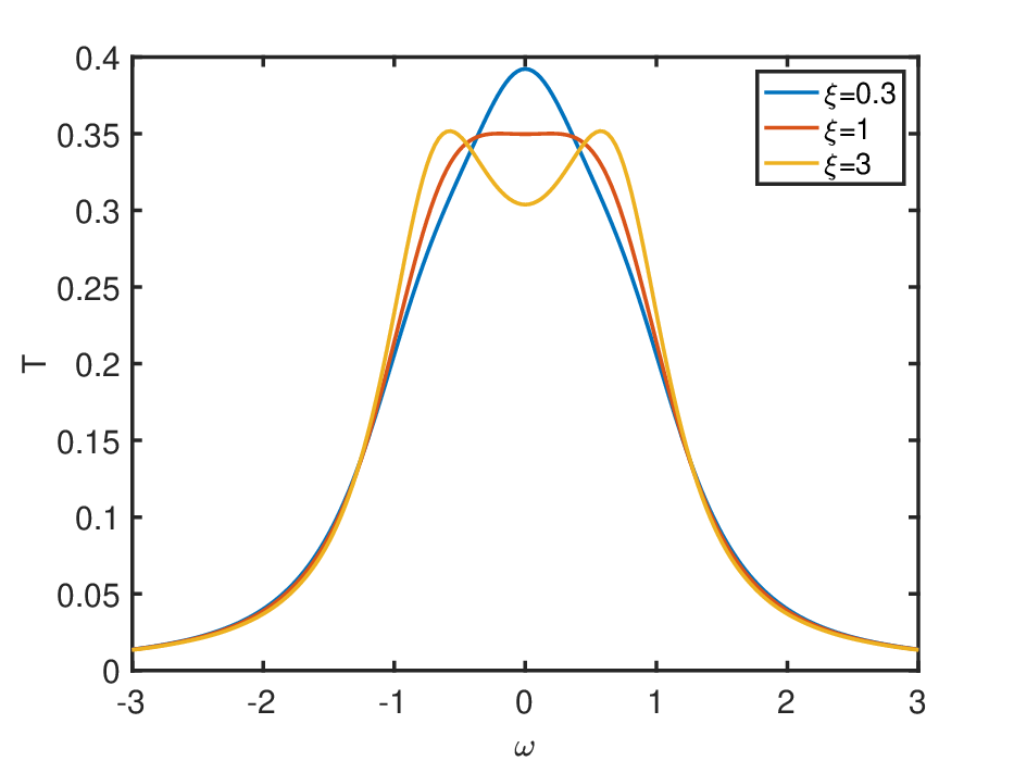
can be neglected ( $\alpha=0$ ). Fig. 1 shows how the transmission scales with electron-rotational coupling $\lambda$ . The transmission is computed numerically using algorithm detailed in Appendix A. For $\lambda=0$ , electronic energy of the molecule is totally decoupled from its rotational motion. Hence the transmission is simply a Lorentzian centered at $\omega=\epsilon$ with a width $\sim\Gamma$ , as described by Eq. (85). If $\lambda$ increases, then Eq. (86) predicts that the resonant value of the electronic transmission decreases, $T(\omega=\epsilon)\sim\lambda^{-3/2}$ , while the transmission starts to exhibit two symmetric maxima at $\omega=\epsilon\pm\omega_{m}$ . Positions of these maxima obey the inequality $\omega_{m}=\sqrt{\lambda^{2}-\Gamma^{2}}<\lambda$ (see Eq. (87)) while the intensity of the transmission in the maxima scales as $T(\omega=\epsilon\pm\omega_{m})\sim\lambda^{-1/2}$ . This behavior of the transmission can be rationalized by the consideration of the problem in the time domain: In the underdamped limit, according to Eq. (80), $R(t)\sim J_{0}(\lambda t)$ and one can anticipate that the oscillation frequency $\approx\lambda$ should manifest itself in the transmission for $\lambda\gg\Gamma_{L},\Gamma_{R}$ .

In terms of physical observation Fig. 1 tells us that in the resonant regime, when molecular orbital energy is aligned with leads Fermi energy, the coupling to the surrounding solvent always suppresses the conductivity of the junction. However, quite oppositely, if the electron transport is dominated by the molecular orbital which is shifted below or above Fermi energy, the solvent may considerably increase the conductance of the system.

Refer to caption — Figure 1: Electronic transmissions $T(\omega)$ computed for various values of electron-rotational coupling $\lambda$ . Parameters used in calculations: $\epsilon=0$ , $\Gamma_{L}=\Gamma_{R}=\xi=1$ . The case of free rotation ( $\alpha=0$ ) is considered here.

There are three characteristic timescales in the system. One is associated with the time of electron tunneling across the molecule, $\Gamma^{-1}$ . The other is the relaxation timescale for solvent dynamics, $\xi^{-1}$ in the underdamped limit and $\xi=D^{-1}$ in the overdamped limit ( $D$ being the diffusion coefficient). The third, $\lambda^{-1}$ , is associated with the electron-rotational coupling and, consequently, with the rate of energy exchange between tunneling electrons and external rotator. Fig. 2 illustrates how $T(\omega)$ is affected by the these timescales. As $\xi$ increases relative to $\Gamma$ , $T(\omega)$ exhibits a transformation from a single-peak to a double-peak structure. This somewhat counterintuitive behavior can be understood from the following considerations. In the limit $\lambda\gg 1$ and $\xi<\lambda$ , the transmission is quite accurately described by the bath-free formula of Eq. (83), which has been analyzed above. For $\lambda<1$ and $\xi<1$ (underdamped limit) $T(\omega)$ is also rather insensitive to $\xi$ : the rotational friction quenches slightly the amplitude of oscillations in $R(t)\sim J_{0}(\lambda t)$ , while the shape of $T(\omega)$ is largely determined by the coupling to the leads, through the exponentially decaying factor $\exp(-\Gamma\tau)$ as given in Eq. (38). The situation changes in the overdamped limit ( $\xi\gg\lambda$ ). In this case, $T(\omega)$ can be evaluated analytically (see Appendix B). Eq. (78) reveals then: the higher the friction, the more pronounced the peaks of $T(\omega)$ . For $\lambda\ll 1$ , for example, Eq. (78) reduces to

\tilde{\rho}_{0}(s)\approx\frac{s+\xi^{-1}}{s^{2}+s\xi^{-1}+\lambda^{2}/2}.

(59)

The expression on the right has two simple poles at $(-\xi^{-1}\pm\sqrt{\xi^{-2}-2\lambda^{2}})/2$ . For $\lambda>/(\sqrt{2}\xi)$ the poles become complex. Their imaginary part, which determines the $T(\omega)$ maxima $\omega_{m}=\sqrt{2\lambda^{2}-\xi^{-2}}/2$ , increases with friction, reaching a value of $\omega_{m}=\lambda/\sqrt{2}<\lambda$ in the overdamped limit $\xi\rightarrow\infty$ . Then, if the broadening of the transmission induced by the coupling to the leads is not too high ( $\Gamma<\omega_{m}$ ) or, equivalently, the electron tunneling time is not too short, $T(\omega)$ exhibits the double-peak structure. In the context of the possibility to manipulate molecular conductivity, Fig. 2 reveals that the viscosity of the solvent can be used as effective control parameter for electron transport properties of molecular junction.

The effect of the external potential is illustrated by Fig. 3, which shows $T(\omega)$ for different $\lambda$ in the presence of the aligning potential (58) with $\alpha=1$ and $\phi_{0}=0$ . Evidently, $U(\phi)$ breaks the rotational symmetry of the transmission, making the angles of $\pm\phi$ inequivalent. Hence the transmission develops particle-hole asymmetry, and $T(\omega)$ has very different behavior for hole ( $\omega<E_{F}$ ) and electron ( $\omega>E_{F}$ ) transport. The particle-hole asymmetry becomes more profound as the strength of electron-rotation coupling $\lambda$ increases, producing a pronounced maximum at positive $\omega$ . As in the case of free rotation shown in Fig. 1, the shift of the peak relative to the molecular orbital energy is determined by the electron-rotational coupling $\lambda$ . The asymmetry depends on the aligning angle $\phi_{0}$ : If $\phi=\pi$ is chosen, the peak of $T(\omega)$ is shifted to hole rather than electron region.

IV conclusions

In this paper, we have developed a quantum transport theory which includes dynamical effects of solvent-molecule interaction in the non-equilibrium Green’s function calculations of electric current. The solvent is considered as a classical macroscopic dipole moment which reorients stochastically and interacts with the electrons tunneling through the molecular junctions. This dynamical electron-rotation interaction makes the quantum mechanical Hamiltonian explicitly time-dependent. The Keldysh-Kadanoff-Baym equations are solved in time-domain. The obtained expression for electric current requires the averaging over realisations of stochastic process related to the dipole moment rotation. The averaging over random realisations of rotational variables is performed using Furutsu-Novikov method to close hierarchy of equations for stochastic correlation functions.

We applied the theory for a model molecular junction - a single molecular orbital coupled to classical rotating dipole via electrostatic interaction. Our calculations shows that, in the resonant regime when molecular orbital energy is aligned with the leads Fermi energy, coupling to the surrounding solvent always suppresses the conductivity of the junction. However, if the electron transport is controlled by the molecular orbital which is shifted below or above Fermi energy, the solvent may noticeably increase the conductance of the system. It is found that the viscosity of the solvent can be used as very effective stimulus to control electron transport properties of molecular junction. If the rotation of the dipole moment is subjected to external aligning potential, the solvent breaks particle-hole symmetry of electron transport favouring holes or electron transport channel depending upon the aligning angle.

Acknowledgment M.F.G. acknowledges support of Hangzhou Dianzi University through the startup funding.

DATA AVAILABILITY

The data that supports the findings of this study are available within the article.

Appendix A Numerical method

For obtaining a matrix form of (55), we use Hermit polynomials $H_{n}(\Omega)$ to expand $\rho(\phi,\Omega,t)$ in a series as

\rho(\phi,\Omega,t)=\sum_{k=-\infty}^{\infty}\,\sum_{n=0}^{\infty}e^{-ik\phi}g_{n}(\Omega)\rho_{kn}(t).

(60)

where

g_{n}(\Omega)=\frac{1}{n!}H_{n}(\Omega)\rho_{B}(\Omega),

(61)

and

\int_{-\infty}^{\infty}d\Omega H_{m}(\Omega)g_{n}(\Omega)=\delta_{mn}.

(62)

Then:

\int_{-\infty}^{\infty}d\Omega H_{m}(\Omega)\partial_{\Omega}g_{n}(\Omega)=-m\delta_{m-1,n}.

(63)

\int_{-\infty}^{\infty}d\Omega H_{m}(\Omega)\Omega g_{n}(\Omega)=m\delta_{m-1,n}+\delta_{m+1,n}.

(64)

\int_{-\infty}^{\infty}d\Omega H_{m}(\Omega)\left(\partial_{\Omega}\Omega+\partial_{\Omega}^{2}\right)g_{n}(\Omega)=-m\delta_{m,n}.

(65)

Hence:

\partial_{t}\rho_{kn}(t)=-i\epsilon\rho_{kn}(t)+i\frac{\lambda}{2}\left[\rho_{k+1,n}(t)+\rho_{k-1,n}(t)\right]\\ +ik\left[\rho_{k,n+1}(t)+n\rho_{k,n-1}(t)\right]\\ +i\frac{\alpha}{2}n\left[e^{-i\phi_{0}}\rho_{k+1,n-1}(t)-e^{i\phi_{0}}\rho_{k-1,n-1}(t)\right]-\xi n\rho_{kn}(t).

(66)

It should be solved with the initial condition

\rho_{kn}(0)=\rho_{k}^{(0)}\delta_{n0}

(67)

where

\rho_{k}^{(0)}=\frac{1}{2\pi}\int_{0}^{2\pi}d\phi e^{ik\phi}\rho_{B}(\phi)

(68)

Evidently,

R(t)=\rho_{00}(t).

(69)

Appendix B Overdamped limit: Analytical expression for electronic transmission

In the overdamped limit ( $\xi\gg 1$ ) the Fokker-Planck equation (55) reduces to the rotational diffusion equation

\partial_{t}\rho(\phi,t)=\left(-ih(\phi)+\xi^{-1}\left(\partial_{\phi}^{2}-\partial_{\phi}G(\phi)\right)\right)\rho(\phi,t).

(70)

In the case of free rotation ( $G(\phi)=0$ , $\alpha=0$ ) this equation can be solved analytically. Expanding $\rho(\phi,t)$ in Fourier series,

\rho(\phi,t)=\sum_{k=-\infty}^{\infty}e^{-ik\phi}\rho_{k}(t),

(71)

we obtain

\partial_{t}\rho_{k}(t)=-i\epsilon\rho_{k}(t)+i\frac{\lambda}{2}\left[\rho_{k+1}(t)+\rho_{k-1}(t)\right]-\xi^{-1}k^{2}\rho_{k}(t),

(72)

\rho_{k}(0)=\delta_{0k}.

(73)

We wish to evaluate

R(t)=\rho_{0}(t).

(74)

By introducing the Laplace transform

\tilde{\rho}_{k}(s)=\int_{0}^{\infty}dte^{-st}\rho_{k}(t),

(75)

we can rewrite Eq. (72) through the three-term recurrence relations

-\delta_{0k}=a_{k}\tilde{\rho}_{k}(s)+b_{k}\tilde{\rho}_{k+1}(s)+c_{k}\tilde{\rho}_{k-1}(s)

(76)

where

a_{k}=-(s_{\epsilon}+\xi^{-1}k^{2}),\,\,b_{k}=c_{k}=i\frac{\lambda}{2},\,\,s_{\epsilon}\equiv s+i\epsilon.

(77)

These recurrence relations can be solved through the continued fraction:

\tilde{\rho}_{0}(s)=\cfrac{1}{s_{\epsilon}+\cfrac{\lambda^{2}/2}{s_{\epsilon}+\xi^{-1}+\cfrac{\lambda^{2}/4}{s_{\epsilon}+4\xi^{-1}+\cfrac{\lambda^{2}/4}{s_{\epsilon}+9\xi^{-1}+...}}}}.

(78)

Then,

T(\omega)=\frac{1}{\pi}\frac{\Gamma_{L}\Gamma_{R}}{\Gamma_{L}+\Gamma_{R}}\mathrm{Re}\tilde{\rho}_{0}\left(i(\omega+\epsilon)+\Gamma\right).

(79)

Appendix C Frictionless rigid rotor: analytical results for electronic transmission

If $\xi=0$ , Eq. (36) can be evaluated analytically:

R(t)=e^{-i\epsilon t}\int_{-\infty}^{\infty}d\Omega\rho_{B}(\Omega)\int_{0}^{2\pi}\frac{d\phi}{2\pi}e^{i\lambda\int_{0}^{t}dt_{1}\cos(\phi+\Omega t_{1})}\\ =e^{-i\epsilon t}\int_{0}^{2\pi}\frac{d\phi}{2\pi}e^{i\lambda t\cos(\phi)}=e^{-i\epsilon t}J_{0}(\lambda t),

(80)

where $J_{0}(x)$ is the Bessel function of the first kind. Since

J_{0}(\lambda t)\approx\sqrt{\frac{2}{\pi\lambda t}}\cos(\lambda t-\pi/4)

(81)

for large $t$ , $R(t)$ exhibits algebraically damped oscillations with a period $2\pi/\lambda$ (for $\epsilon=0$ ).

The transmission of Eq. (38) can be evaluated as follows:

T(\omega)=\mathrm{Re}\int_{0}^{\infty}dte^{-\Gamma t}e^{-i(\epsilon-\omega)t}\int_{0}^{2\pi}d\phi e^{i\lambda t\cos(\phi)}\\ =\mathrm{Re}\int_{0}^{2\pi}d\phi\frac{1}{\Gamma+i(\epsilon-\omega-\lambda\cos(\phi))}\\ =\frac{2\pi}{\Gamma}\mathrm{Re}\frac{1}{\sqrt{\left[\Gamma+i(\epsilon-\omega)\right]^{2}+\lambda^{2}}}.

(82)

Explicitly,

T(\omega)=\frac{2\pi}{\Gamma}\sqrt{\frac{2\Gamma^{2}-z+\sqrt{z^{2}+4\lambda^{2}\Gamma^{2}}}{2(z^{2}+4\lambda^{2}\Gamma^{2})}}.

(83)

where

z=(\epsilon-\omega)^{2}+\Gamma^{2}-\lambda^{2}.

(84)

In two particular cases, much simpler and easier-to-grasp formulas are deducible from Eq. (83). If $\Gamma\gg\lambda$ , the transmission is described by the Lorentzian centered at $\omega=\epsilon$ ,

T(\omega)\sim\frac{\Gamma}{(\epsilon-\omega)^{2}+\Gamma^{2}}.

(85)

In the opoosite limit $\lambda\gg\Gamma$ , the transmission exhibits two symmetric maxima positioned at $\epsilon-\omega=\pm\omega_{m}$ :

T(\omega)\sim\sqrt{\frac{\lambda\Gamma}{((\epsilon-\omega)^{2}-\omega_{m}^{2})^{2}+4\lambda^{2}\Gamma^{2}}}

(86)

with

\omega_{m}=\sqrt{\lambda^{2}-\Gamma^{2}}.

(87)

References

Xiang et al. (2016) D. Xiang, X. Wang, C. Jia, T. Lee, and X. Guo, Chemical Reviews 116, 4318 (2016), pMID: 26979510, eprint https://doi.org/10.1021/acs.chemrev.5b00680, URL https://doi.org/10.1021/acs.chemrev.5b00680.
Wu et al. (2008) S. Wu, M. T. González, R. Huber, S. Grunder, M. Mayor, C. Schönenberger, and M. Calame, Nature Nanotechnology 3, 569 (2008), URL https://doi.org/10.1038/nnano.2008.237.
Nishino et al. (2013) T. Nishino, N. Hayashi, and P. T. Bui, Journal of the American Chemical Society 135, 4592 (2013), pMID: 23488642, eprint https://doi.org/10.1021/ja311463b, URL https://doi.org/10.1021/ja311463b.
Bui et al. (2013) P. T. Bui, T. Nishino, Y. Yamamoto, and H. Shiigi, Journal of the American Chemical Society 135, 5238 (2013), pMID: 23534478, eprint https://doi.org/10.1021/ja312019p, URL https://doi.org/10.1021/ja312019p.
Kuznetsov (2007) A. M. Kuznetsov, J. Chem. Phys. 127, 084710 (2007).
Milan et al. (2016) D. C. Milan, O. A. Al-Owaedi, M.-C. Oerthel, S. Marqués-González, R. J. Brooke, M. R. Bryce, P. Cea, J. Ferrer, S. J. Higgins, C. J. Lambert, et al., The Journal of Physical Chemistry C 120, 15666 (2016), eprint https://doi.org/10.1021/acs.jpcc.5b08877, URL https://doi.org/10.1021/acs.jpcc.5b08877.
Dzhioev and Kosov (2012) A. A. Dzhioev and D. S. Kosov, Phys. Rev. B 85, 033408 (2012), URL https://link.aps.org/doi/10.1103/PhysRevB.85.033408.
Leary et al. (2009) E. Leary, H. Höbenreich, S. J. Higgins, H. van Zalinge, W. Haiss, R. J. Nichols, C. M. Finch, I. Grace, C. J. Lambert, R. McGrath, et al., Phys. Rev. Lett. 102, 086801 (2009), URL https://link.aps.org/doi/10.1103/PhysRevLett.102.086801.
Stipe et al. (1997) B. C. Stipe, M. A. Rezaei, W. Ho, S. Gao, M. Persson, and B. I. Lundqvist, Phys. Rev. Lett. 78, 4410 (1997).
Luka-Guth et al. (2016) K. Luka-Guth, S. Hambsch, A. Bloch, P. Ehrenreich, B. M. Briechle, F. Kilibarda, T. Sendler, D. Sysoiev, T. Huhn, A. Erbe, et al., Beilstein J. Nanotechnol. 7, 1055 (2016).
Kotiuga et al. (2015) M. Kotiuga, P. Darancet, C. R. Arroyo, L. Venkataraman, and J. B. Neaton, Nano Letters 15, 4498 (2015), URL https://doi.org/10.1021/acs.nanolett.5b00990.
Fatemi et al. (2011) V. Fatemi, M. Kamenetska, J. B. Neaton, and L. Venkataraman, Nano Letters 11, 1988 (2011), pMID: 21500833, eprint https://doi.org/10.1021/nl200324e, URL https://doi.org/10.1021/nl200324e.
Ghane et al. (2015) T. Ghane, A. Kleshchonok, R. Gutierrez, and G. Cuniberti, The Journal of Physical Chemistry C 119, 20201 (2015), eprint https://doi.org/10.1021/acs.jpcc.5b06867, URL https://doi.org/10.1021/acs.jpcc.5b06867.
Choi et al. (2016) B. Choi, B. Capozzi, S. Ahn, A. Turkiewicz, G. Lovat, C. Nuckolls, M. L. Steigerwald, L. Venkataraman, and X. Roy, Chem. Sci. 7, 2701 (2016), URL http://dx.doi.org/10.1039/C5SC02595H.
Kornyshev et al. (2006) A. A. Kornyshev, A. M. Kuznetsov, and J. Ulstrup, Proceedings of the National Academy of Sciences 103, 6799 (2006), eprint https://www.pnas.org/content/103/18/6799.full.pdf, URL https://www.pnas.org/content/103/18/6799.
Zhang et al. (2008) J. Zhang, A. M. Kuznetsov, I. G. Medvedev, Q. Chi, T. Albrecht, P. S. Jensen, and J. Ulstrup, Chemical Reviews 108, 2737 (2008), pMID: 18620372, eprint https://doi.org/10.1021/cr068073+, URL https://doi.org/10.1021/cr068073+.
Klyatskin (2005) V. I. Klyatskin, Dynamics of Stochastic Systems (Amsterdam: Elsevier, 2005).
Coffey et al. (1996) W. T. Coffey, Y. P. Kalmykov, and J. Waldron, The Langevin Equation: With Applications in Physics, Chemistry and Electrical Engineering (World Scientific, Singapore, 1996).
Haug and Jauho (2010) H. Haug and A. Jauho, Quantum Kinetics in Transport and Optics of Semiconductors (Springer, Berlin/Heidelberg, 2010).
Van Kampen (2007) N. G. Van Kampen, Stochastic Processes in Physics and Chemistry (3th ed. Amsterdam: North-Holland Personal Library, 2007).