跳到论文正文
W Papers独立论文阅读器 arXiv:2012.01049 论文正文 计算阅读时间 · 0%
引用这篇论文根据当前论文元数据生成,正式投稿前建议核对。


License: CC BY-NC-ND 4.0
arXiv:2012.01049v2 [math.NA] 14 Aug 2022

On Planar Polynomial Geometric InterpolationJournal: Journal of Approximation Theory

Jernej Kozak Email: jernej.kozak@fmf.uni-lj.si URL: https://arhiv-www.fmf.uni-lj.si/˜kozak/wikiang/
index.php?title=Main_Page
Note: The author acknowledges the financial support from the Slovenian Research Agency (research core funding No.P1-0291)
Abstract

In the paper, the planar polynomial geometric interpolation of data points is revisited. Simple sufficient geometric conditions that imply the existence of the interpolant are derived in general. They require data points to be convex in a certain discrete sense. Since the geometric interpolation is based precisely on the known data only, one may consider it as the parametric counterpart to the polynomial function interpolation. The established result confirms the Höllig-Koch conjecture on the existence and the approximation order in the planar case for parametric polynomial curves of any degree stated quite a while ago.

Keywords: 
polynomial curve , geometric interpolation , existence , approximation order
2010 MSC
41A10 , 65D05 , 65D17

1 Introduction

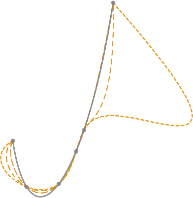
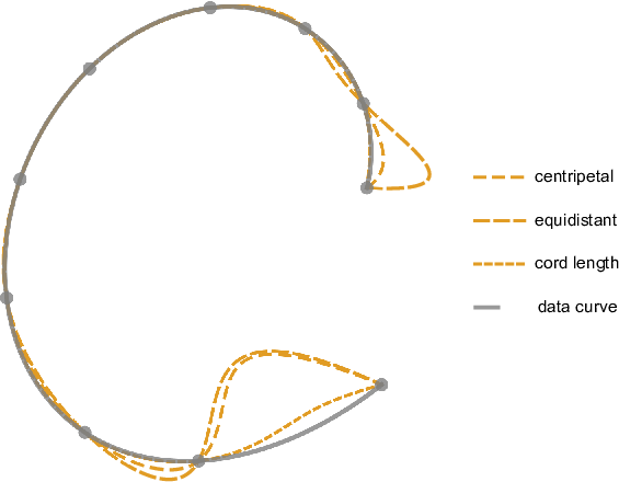
The study of geometric polynomial interpolation problems was initiated in [1] where Hermite cubic interpolation of two points, tangent directions, and curvatures was analyzed. It soon became apparent that geometric interpolation brings two important practical advantages compared to linear polynomial interpolation schemes adapted to the curve case. First, the interpolating curve depends on geometric quantities only: data points, tangent directions, curvatures, etc. As to the second one, we avoid the choice of parametrization in advance. This allows us to stick to lower degree polynomials, but use the implicit parametrization to keep the approximation power of the higher degree component-wise linear interpolants. In practical applications, the shape of an interpolating curve is often an issue. One would require that the interpolant at least roughly preserves the shape of the data it is based upon. However, a priori choice of parametrization combined with higher degree polynomials may make this goal hard to achieve. As an example, consider the points, sampled from smooth convex curves (Fig. 1). With three commonly used parametrizations applied, none of the interpolants is satisfying. But the same data interpolated geometrically, determine quite differently a satisfactory curve approximation (Fig. 2). So understandably a lot of work that followed [1] investigated the geometric interpolation quite thoroughly. The problems considered included Lagrange interpolation of data points only, and its limit case, Hermite, where also data directions, data curvatures, etc. are prescribed. If all data appear at one point, the Hermite case reduces to a Taylor one.

Refer to caption
Refer to caption
Figure 1: Examples of data interpolated by a polynomial parametric curve with parametrization chosen in advance. Both data curves are smooth and convex.

But the problems involved are generally nonlinear, so the existence, the approximation order, and the construction are the burning issues. The asymptotic approach was often the tool to tackle the first two goals. There, the data is assumed to be taken from a sufficiently small part of a convex curve that could be locally parametrized by one of the components.

In [2], a natural conjecture on the geometric polynomial interpolation was made, based upon the authors’ previous work and results referenced therein. This conjecture in the special, Lagrange planar case, predicts that a polynomial curve of degree≤n{\textrm{degree}\ \leq n} can if some appropriate assumptions are met interpolate 2​n2n points, with optimal approximation order 2​n2n. The conjecture was confirmed in some particular cases, mostly for low degree polynomials, and in the asymptotic sense only [1, 3, 2, 4, 5, 6, 7, et al.].

It is somewhat surprising how long the result for the general degree curves was slipping one’s hands. In this paper, we close this gap for the planar Lagrange interpolation problem, and we present quite general geometric conditions that assure both the existence and the optimal approximation order for arbitrary degree cases. Recently, a similar, positive result for the Taylor case polynomial curve expansion was given in [8] for quite a large infinite subset of ℕ\mathbb{N}.

The result of the paper is based on an old but far-reaching achievement developed to the Bolzano–Poincaré–Miranda theorem for simplices in [9, Theorem 2.1]: if a set of continuous functions satisfies certain sign conditions at the simplex boundary, it must vanish at some interior point of the simplex.

The outline of the paper is as follows. In Section 2, the Lagrange interpolation problem is defined, and the main theorems are listed. In Section 3, the functions and the corresponding equations to be solved are derived. Section 4, the most technical part, contains the analysis of the functions involved. Based upon Section 4 the last two sections provide the proofs of the theorems given in Section 2.

2 Lagrange interpolation problem

The Lagrange interpolation problem is formulated as follows. Suppose that a sequence of 2​n2n distinct points

𝑷ℓ=(aℓbℓ)∈ℝ2,ℓ=0,1,…,2n−1,𝒂:=(aℓ)ℓ=02​n−1,𝒃:=(bℓ)ℓ=02​n−1,{\boldsymbol{P}}_{\ell}=\begin{pmatrix}a_{\ell}\cr b_{\ell}\end{pmatrix}\in\mathbb{R}^{2},\ \ell=0,1,\dots,2n-1,\quad\boldsymbol{a}:=\left(a_{\ell}\right)_{\ell=0}^{2n-1},\ \boldsymbol{b}:=\left(b_{\ell}\right)_{\ell=0}^{2n-1}, (1)

is given. Find a parametric polynomial curve

𝒑n:[0,1]→ℝ2\boldsymbol{p}_{n}:[0,1]\to\mathbb{R}^{2}

of degree ≤n\leq n that interpolates the given data points (1) at some parameter values tℓ∈[0,1]{t_{\ell}\in[0,1]} in increasing order, i.e.,

𝒑n(tℓ)=𝑷ℓ,ℓ=0,1,…,2n−1.\boldsymbol{p}_{n}\left(t_{\ell}\right)={\boldsymbol{P}}_{\ell},\quad\ell=0,1,\dots,2n-1. (2)

Since a linear reparametrization preserves the degree of a parametric polynomial curve, one can assume t0:=0t_{0}:=0 and t2​n−1:=1t_{2n-1}:=1, but the remaining parameters

𝒕:=(tℓ)ℓ=12​n−2{\boldsymbol{t}}:=\left(t_{\ell}\right)_{\ell=1}^{2n-2}

are unknown, ordered as

t0=0<t1<⋯<t2​n−2<t2​n−1=1.t_{0}=0<t_{1}<\dots<t_{2n-2}<t_{2n-1}=1.

Let Δ\Delta denote the forward difference, i.e.,

Δ​wℓ:=wℓ+1−wℓ,Δ​𝑷ℓ:=𝑷ℓ+1−𝑷ℓ.\Delta w_{\ell}:=w_{\ell+1}-w_{\ell},\quad\Delta\boldsymbol{P}_{\ell}:={\boldsymbol{P}}_{\ell+1}-{\boldsymbol{P}}_{\ell}.

We have the following assertion.

Theorem 1

If, possibly after a linear transformation, the differences

Δ​aℓ,Δ​bℓ,ℓ=0,1,…,2​n−2,\displaystyle\Delta{a}_{\ell},\ \Delta{b}_{\ell},\quad\ell=0,1,\dots,2n-2, (3)

of the data (1) are all positive or all negative and the determinants

‖Δ​𝑷ℓ−1Δ​𝑷ℓ‖=Δaℓ−1Δbℓ−ΔaℓΔbℓ−1,ℓ=1,2,…,2n−2,\displaystyle\begin{Vmatrix}\Delta\boldsymbol{P}_{\ell-1}&\!\!\!\Delta\boldsymbol{P}_{\ell}\end{Vmatrix}=\Delta{a}_{\ell-1}\Delta{b}_{\ell}-\Delta{a}_{\ell}\Delta{b}_{\ell-1},\quad\ell=1,2,\dots,2n-2, (4)

are all of the same sign, the interpolation problem (2) has at least one solution.

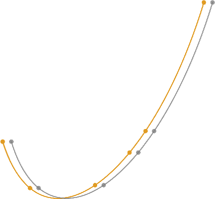
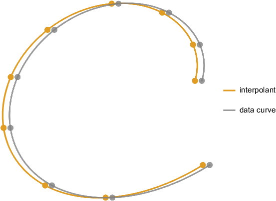
Some obvious remarks are right on the spot. Even if the data (1) don’t satisfy the assumptions (3) and (4), they may be satisfied after a proper linear data transformation. In particular, the role of both data components may be reversed, any data rotation or reflection is allowed, etc. All of the asymptotic approaches to the interpolation problem are covered here too. Generally, Theorem 1 gives the positive answer for all data that could be transformed to a sampled monotone convex function curve by an affine transformation, as is the data case on Fig. 2 (left). But the right side of the same figure requires more general assumptions.

Refer to caption
Refer to caption
Figure 2: Data that satisfy Theorem 1 interpolated by a cubic parametric curve (left), and data that satisfy Theorem 2 and corresponding polynomial interpolant of degree 55 (right). Data curves are plotted with a small offset to the right since otherwise, any distinction between the original curve and its interpolant would not be visible.
Theorem 2

If the determinants

‖Δ​𝑷j−1+kΔ​𝑷j−1+ℓ‖,j=1,2,…,n−1; 0≤k<ℓ≤n,\begin{Vmatrix}\Delta\boldsymbol{P}_{j-1+k}&\!\!\Delta\boldsymbol{P}_{j-1+\ell}\end{Vmatrix},\quad j=1,2,\dots,n-1;\,0\leq k<\ell\leq n, (5)

are all of the same sign, the interpolation problem (2) has at least one solution.

Note that the assumptions (5) are affinely invariant. The proof of Theorem 1 will carry most of the burden, and Theorem 2 will be confirmed with its help. There is little hope that simple necessary and sufficient conditions that guarantee existence could be found in general. In the case n=2n=2 the geometric interpolation problem has a solution iff (5) are satisfied as observed already in [10] and further elaborated in [11]. This case was generalized, together with necessary and sufficient conditions for the existence of the interpolant, to any dimension in [6] where a particular form of (5) already appeared. But if the degree nn is larger, i.e., n≥3n\geq 3 in the planar case, the analysis of all possibilities becomes very complicated even for planar cubic interpolation [12, 13]. If the data are not convex in the discrete sense of either one of the theorems, the existence of the solution depends heavily on the particular data set. One would expect that the results carry over to the Hermite interpolation problems, but we leave the confirmation to the future work.

3 Equations of the problem

As a vector in ℝ2​n−2\mathbb{R}^{2n-2}, the unknowns 𝒕{\boldsymbol{t}} should belong to the interior int​(𝒮)\textrm{int}\left(\mathcal{S}\right) of a (2​n−2){(2n-2)}-simplex 𝒮\mathcal{S},

𝒮:={𝒕∈ℝ2​n−2|0≤t1≤⋯≤t2​n−2≤1}.\mathcal{S}:=\left\{{\boldsymbol{t}}\in\mathbb{R}^{2n-2}|0\leq t_{1}\leq\dots\leq t_{2n-2}\leq 1\right\}.

The system of equations (2) has to determine the unknown 𝒑n\boldsymbol{p}_{n} as well as the parameters 𝒕{\boldsymbol{t}}. But the two tasks can be separated if one can provide enough linearly independent functionals, depending on 𝒕{\boldsymbol{t}} only, that map 𝒑n\boldsymbol{p}_{n} to zero. Divided differences, based upon ≥n+2\geq~n+2 values, are a natural choice. Let us apply the divided differences

[tj−1,tj,…,tn+j],j=1,2,…,n−1,[t_{j-1},t_{j},\dots,t_{n+j}],\quad j=1,2,\dots,n-1, (6)

to both sides of (2). Since deg⁡𝒑n≤n{\deg\ \boldsymbol{p}_{n}\leq n}, the left side vanishes, and so should the right one. But the parameters tℓt_{\ell} are distinct and this condition becomes

∑ℓ=j−1n+j1∏m=j−1m≠ℓn+j(tℓ−tm)𝑷ℓ=0,j=1,2,…,n−1.\displaystyle{\sum_{\ell=j-1}^{n+j}\frac{1}{\prod\limits_{\genfrac{}{}{0.0pt}{}{m=j-1}{m\ne\ell}}^{n+j}(t_{\ell}-t_{m})}}\ \boldsymbol{P}_{\ell}=0,\quad j=1,2,\dots,n-1. (7)

This nonlinear system depends on the data 𝑷ℓ\boldsymbol{P}_{\ell} and the unknowns 𝒕{\boldsymbol{t}} only. If the solution 𝒕∈int​(𝒮){{\boldsymbol{t}}\in\textrm{int}\left(\mathcal{S}\right)} is found, one can apply any algorithm inherited from the polynomial function interpolation to construct the interpolatory curve 𝒑n\boldsymbol{p}_{n} component-wise. For each jj the system (7) provides two equations based upon the first and the second component of the data. For our purpose, it will be more convenient to rewrite (7) in a polynomial form. However, from a computational point of view, the equations (7) are less sensitive to numerical cancellation, and they produced the examples of Fig. 2 in a couple of Newton steps starting with an equidistant initial guess. Let V⁡(tj1,…,tjr)V\!\!\left(t_{j_{1}},\dots,t_{j_{r}}\right) be a Vandermonde determinant based upon tj1,…,tjrt_{j_{1}},\dots,t_{j_{r}},

V⁡(tj1,…,tjr):=‖tjℓi−1‖i=1;ℓ=1r;r=∏ℓ=1r∏i=1ℓ−1(tjℓ−tji),V\!\!\left(t_{j_{1}},\dots,t_{j_{r}}\right):=\begin{Vmatrix}t_{j_{\ell}}^{i-1}\end{Vmatrix}_{i=1;\ell=1}^{r;r}=\prod_{\ell=1}^{r}\prod_{i=1}^{\ell-1}\left(t_{j_{\ell}}-t_{j_{i}}\right), (8)

and let

V⁡(tj1,…,tjr,cj1,…,cjr)V\!\!\left(t_{j_{1}},\dots,t_{j_{r}};c_{j_{1}},\dots,c_{j_{r}}\right)

denote a determinant, obtained from (8) by replacing the last determinant row
(tj1r−1,…,tjrr−1){\left(t_{j_{1}}^{r-1},\dots,t_{j_{r}}^{r-1}\right)} by the values (cj1,…,cjr)\left(c_{j_{1}},\dots,c_{j_{r}}\right),

V⁡(tj1,…,tjr,cj1,…,cjr)=∑ℓ=1r(−1)r+ℓ​cjℓ​V​(tj1,…,tjℓ−1,tjℓ+1,…,tjr).V\!\!\left(t_{j_{1}},\dots,t_{j_{r}};c_{j_{1}},\dots,c_{j_{r}}\right)=\sum_{\ell=1}^{r}\left(-1\right)^{r+\ell}c_{j_{\ell}}V\!\!\left(t_{j_{1}},\dots,t_{j_{\ell-1}},t_{j_{\ell+1}},\dots,t_{j_{r}}\right).

The divided difference (6) applied to a sequence (cℓ)ℓ=j−1ℓ=n+j\left(c_{\ell}\right)_{\ell=j-1}^{\ell=n+j} as a quotient of the Vandermonde determinants reads

V⁡(tj−1,…,tn+j,cj−1,…,cn+j)V⁡(tj−1,…,tn+j).\frac{V\!\!\left(t_{j-1},\dots,t_{n+j};c_{j-1},\dots,c_{n+j}\right)}{V\!\!\left(t_{j-1},\dots,t_{n+j}\right)}.

Thus, if we multiply (7) by V⁡(tj−1,…,tn+j)V\!\!\left(t_{j-1},\dots,t_{n+j}\right) we obtain the polynomial form of the system

f𝒂,j​(tj−1,…,tn+j)=0,\displaystyle f_{\boldsymbol{a},j}\left(t_{j-1},\dots,t_{n+j}\right)=0,
j=1,2,…,n−1,\displaystyle\quad\quad\quad\quad\quad\quad\quad\quad\quad\quad\quad j=1,2,\dots,n-1, (9)
f𝒃,j​(tj−1,…,tn+j)=0,\displaystyle f_{\boldsymbol{b},j}\left(t_{j-1},\dots,t_{n+j}\right)=0,

where

f𝒄,j​(tj−1,…,tn+j):=V⁡(tj−1,…,tn+j,cj−1,…,cn+j).f_{\boldsymbol{c},j}\left(t_{j-1},\dots,t_{n+j}\right):=V\!\!\left(t_{j-1},\dots,t_{n+j};c_{j-1},\dots,c_{n+j}\right).

Here and throughout the paper, coefficients 𝒄\boldsymbol{c} will be used as a placeholder for either 𝒂\boldsymbol{a} or 𝒃\boldsymbol{b} meaning that any relation or text involving 𝒄\boldsymbol{c} holds for either of them. Note that f𝒄,jf_{\boldsymbol{c},j} depends linearly on the constants cj−1,cj,…,cn+jc_{j-1},c_{j},\dots,c_{n+j} only. It is also invariant under data translation since divided differences map constants to zero. So f𝒄,jf_{\boldsymbol{c},j} depends linearly on data differences Δ​cℓ\Delta{c}_{\ell},

f𝒄,j​(tj−1,…,tn+j)=\displaystyle f_{\boldsymbol{c},j}\left(t_{j-1},\dots,t_{n+j}\right)=
=∑k=jn+j(−1)n+j−k​(ck−cj−1)​V​(tj−1,…,tk−1,tk+1,…,tn+j)\displaystyle\quad=\sum_{k=j}^{n+j}\left(-1\right)^{n+j-k}(c_{k}-c_{j-1})V\!\!\left(t_{j-{1}},\dots,t_{{k-1}},t_{{k+1}},\dots,t_{n+j}\right) (10)
=∑r=jn+jΔ​cr−1​∑k=rn+j(−1)n+j−k​V​(tj−1,…,tk−1,tk+1,…,tn+j).\displaystyle\quad=\sum_{r=j}^{n+j}\Delta{c}_{r-1}\sum_{k=r}^{n+j}\left(-1\right)^{n+j-k}V\!\!\left(t_{j-{1}},\dots,t_{{k-1}},t_{{k+1}},\dots,t_{n+j}\right).

This shows that the equations derived follow the affine nature of the interpolation problem, and it explains the following remark.

Remark 1

For each jj separately, 1≤j≤n−11\leq j\leq n-1, we may replace the data

(Δ​𝑷j−1Δ​𝑷j…Δ​𝑷n+j−1)\begin{pmatrix}\Delta\boldsymbol{P}_{j-1}&\Delta\boldsymbol{P}_{j}&\dots&\Delta\boldsymbol{P}_{n+j-1}\end{pmatrix} (11)

which in (3) determine the function pairs f𝐚,jf_{\boldsymbol{a},j}, and f𝐛,jf_{\boldsymbol{b},j}, by

(Aj​Δ​𝑷j−1Aj​Δ​𝑷j…Aj​Δ​𝑷n+j−1),\begin{pmatrix}A_{j}\,\Delta\boldsymbol{P}_{j-1}&A_{j}\,\Delta\boldsymbol{P}_{j}&\dots&A_{j}\,\Delta\boldsymbol{P}_{n+j-1}\end{pmatrix},

where Aj:ℝ2→ℝ2A_{j}:\mathbb{R}^{2}\to\mathbb{R}^{2} is any nonsingular linear transformation. The system of equations generated by the modified functions is equivalent to the original one.

The following remark contributes an error term in case the data are sampled from a data curve.

Remark 2

Suppose that the data

𝑷ℓ=𝒈(ξℓ),ℓ=0,1,…,2n−1,{\boldsymbol{P}}_{\ell}=\boldsymbol{g}(\xi_{\ell}),\ \ell=0,1,\dots,2n-1,

are taken from a smooth parametric curve 𝐠:[ξ0,ξ2​n−1]→ℝ2\boldsymbol{g}:[\xi_{0},\xi_{2n-1}]\to\mathbb{R}^{2} at increasing parameter values ξ0<ξ1<⋯<ξ2​n−1.\xi_{0}<\xi_{1}<\dots<\xi_{2n-1}. If the solution 𝐭∈int​(𝒮)\boldsymbol{t}\in\textrm{int}\left(\mathcal{S}\right) of (3) exists, the function case polynomial interpolation provides the remainder in the parametric one too. Let φ:[0,1]→[ξ0,ξ2​n−1]\varphi:[0,1]\to[\xi_{0},\xi_{2n-1}] be any regular reparametrization of 𝐠\boldsymbol{g} that satisfies

φ(tℓ)=ξℓ,ℓ=0,1,…,2n−1.\varphi(t_{\ell})=\xi_{\ell},\quad\ell=0,1,\dots,2n-1.

Then

𝒈⁡(φ⁡(t))=𝒑n​(t)+(∏ℓ=02​n−1(t−tℓ))​[ξ0,ξ1,…,ξ2​n−1,φ⁡(t)]​𝒈,t∈[0,1].\boldsymbol{g}(\varphi(t))=\boldsymbol{p}_{n}\left(t\right)+\left(\prod_{\ell=0}^{2n-1}\left(t-t_{\ell}\right)\right)\,[\xi_{0},\xi_{1},\dots,\xi_{2n-1},\varphi(t)]\boldsymbol{g},\quad t\in[0,1].

As an example, the normal reparametrization φ\varphi, introduced in [14], is often a sensible choice (Fig. 3).

Refer to caption
Refer to caption
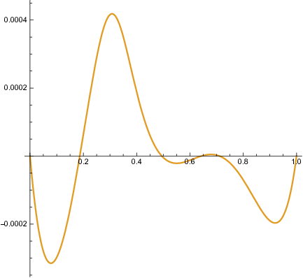
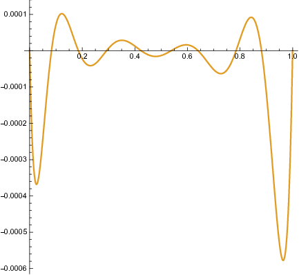
Figure 3: Normal reparametrization φ\varphi and corresponding parametric difference graphs 𝒈∘φ−𝒑\boldsymbol{g}\circ\varphi-\boldsymbol{p} of the examples outlined in Fig. 2.
Remark 3

If the data curve 𝐠\boldsymbol{g} in Remark 2 is additionally convex on [ξa,ξb][\xi_{a},\xi_{b}], the points 𝐏ℓ{\boldsymbol{P}}_{\ell} satisfy the assumptions of Theorem 2 for any increasing choice of parameters ξℓ∈[ξa,ξb]{\xi_{\ell}\in[\xi_{a},\xi_{b}]}. So by [7, Theorem 4.6] the interpolating polynomial parametric curve 𝐩𝐧\boldsymbol{p_{n}} approximates 𝐠\boldsymbol{g} with the optimal approximation order 2​n2n. Fig. 4 shows a numerical estimate of the approximation order for the data of Fig. 2 as a function of shrinking data curve parameter interval computed as in [15, at several spots]. The numerical evidence clearly confirms the expected result, 2​n=6{2n=6} (left), and 2​n=10{2n=10} (right).

Refer to caption
Refer to caption
Figure 4: Numerical estimate of the approximation order for the data of Fig. 2, left and right respectively. The abscissa denotes the length of the data curve parameter relative to the length of the initial one.

4 Analysis of polynomials f𝒄,jf_{\boldsymbol{c},j}

Somewhat sloppy, we shall consider the polynomial f𝒄,jf_{\boldsymbol{c},j} wherever needed also as a function with the domain extended naturally,

f𝒄,j:ℝ2​n−2→ℝ:(tℓ)ℓ=12​n−2↦f𝒄,j​(tj−1,…,tn+j),f_{\boldsymbol{c},j}:\mathbb{R}^{2n-2}\to\mathbb{R}:\,\left(t_{\ell}\right)_{\ell=1}^{2n-2}\mapsto f_{\boldsymbol{c},j}\left(t_{j-1},\dots,t_{n+j}\right),

and

𝒇j:=(f𝒂,j,f𝒃,j)T,𝒇:=(f𝒂,1,f𝒃,1,…,f𝒂,n−1,f𝒃,n−1)T.\boldsymbol{f}_{j}:=\left(f_{\boldsymbol{a},j},f_{\boldsymbol{b},j}\right)^{T}\!,\quad\boldsymbol{f}:=\left(f_{\boldsymbol{a},1},f_{\boldsymbol{b},1},\dots,f_{\boldsymbol{a},n-1},f_{\boldsymbol{b},n-1}\right)^{T}.

This helps us to define varieties 𝒱⁡(f𝒄,j)\mathcal{V}\!\left(f_{\boldsymbol{c},j}\right), 𝒱⁡(𝒇j)\mathcal{V}\!\left(\boldsymbol{f}_{j}\right) and 𝒱⁡(𝒇)\mathcal{V}\!\left(\boldsymbol{f}\right), where the variety definition of a scalar function gg,

𝒱⁡(g):={𝒕∈ℝ2​n−2|g⁡(𝒕)=0},\mathcal{V}\!\left(g\right):=\left\{\boldsymbol{t}\in\mathbb{R}^{2n-2}\,\big|\,g\left(\boldsymbol{t}\right)=0\right\},

is naturally extended to the vector function case 𝒱⁡(𝒈)\mathcal{V}\!\left(\boldsymbol{g}\right). The system (3) is equivalent to (7) except for possible extraneous solutions at the simplex boundary ∂𝒮:=𝒮∖int​(𝒮){\partial\,\mathcal{S}:=\mathcal{S}\setminus\textrm{int}\left(\mathcal{S}\right)}, and there is to prove 𝒱​(𝒇)∩int​(𝒮)≠∅\mathcal{V}\!\left(\boldsymbol{f}\right)\cap\textrm{int}\left(\mathcal{S}\right)\neq\emptyset. Of particular interest will be a variety part

𝒱𝒮​(g):=cl​(𝒱⁡(g)∩int​(𝒮))\mathcal{V}_{\!\mathcal{S}\!\!}\left(g\right):=\textrm{cl}\big(\mathcal{V}\!\left(g\right)\cap\textrm{int}\left(\mathcal{S}\right)\big)

the restriction of 𝒱⁡(g)\mathcal{V}\!\left(g\right) to 𝒮\mathcal{S} that drops out the variety boundary points that can’t be reached from int​(𝒮)\textrm{int}\left(\mathcal{S}\right). The simplex 𝒮\mathcal{S} requires some additional notation. It is a convex hull of points,

𝒮=co​{𝑸0,…,𝑸2​n−2},\mathcal{S}=\textrm{co}\!\left\{\boldsymbol{Q}_{0},\dots,\boldsymbol{Q}_{2n-2}\right\},

where

𝑸ℓ:=(0,…,0⏟ℓ,1,…,1⏟2​n−2−ℓ)T,ℓ=0,1,…,2n−2.\boldsymbol{Q}_{\ell}:=(\underbrace{0,\dots,0}_{\ell},\underbrace{1,\dots,1}_{2n-2-\ell})^{T},\quad\ell=0,1,\dots,2n-2. (12)

The simplex faces will be denoted by

𝒮\{ℓ1,…,ℓr}=co​{𝑸j}j∈{0,…,2​n−2}\{ℓ1,…,ℓr}.\displaystyle\mathcal{S}_{\backslash\left\{\ell_{1},\dots,\ell_{r}\right\}}=\textrm{co}\!\left\{\boldsymbol{Q}_{j}\right\}_{j\in\{0,\dots,2n-2\}\backslash\{\ell_{1},\dots,\ell_{r}\}}.

In this notation, the boundary of the simplex 𝒮\mathcal{S} is determined by the (2​n−3)​-simplex(2n-3)\textrm{-simplex} faces

𝒮\{ℓ},ℓ=0,1,…,2​n−2.\mathcal{S}_{\backslash\left\{\ell\right\}},\quad\ell=0,1,\dots,2n-2. (13)
Refer to caption
Figure 5: The case n=2n=2: the simplex 𝒮⊂ℝ2\mathcal{S}\subset\mathbb{R}^{2}, the points 𝑸0,𝑸1,𝑸2\boldsymbol{Q}_{0},\boldsymbol{Q}_{1},\boldsymbol{Q}_{2}, and the faces 𝒮\{0},𝒮\{1},𝒮\{2}\mathcal{S}_{\backslash\left\{0\right\}},\mathcal{S}_{\backslash\left\{1\right\}},\mathcal{S}_{\backslash\left\{2\right\}}.

The simplest case n=2n=2 is shown in Fig. 5. The first observation is straightforward. Since precisely the components ℓ\ell and ℓ+1{\ell+1} of 𝑸ℓ\boldsymbol{Q}_{\ell} are by (12) distinct, the (2​n−3)(2n-3)-simplex 𝒮\{ℓ}\mathcal{S}_{\backslash\left\{\ell\right\}} is the maximal face of 𝒮\mathcal{S} characterized by tℓ=tℓ+1t_{\ell}=t_{\ell+1}. Given jj, 1≤j≤n−11\leq j\leq n-1, suppose that

j−1≤r1,r2≤n+j−1,r2≠r1,tr2=tr1.j-1\leq r_{1},r_{2}\leq n+j-1,\ r_{2}\neq r_{1},\ \ t_{r_{2}}=t_{r_{1}}.

We then deduce from (3)

f𝒄,j​(tj−1,…,tr2−1,tr1,tr2+1,…,tn+j)=\displaystyle f_{\boldsymbol{c},j}\left(t_{j-1},\dots,t_{r_{2}-1},t_{r_{1}},t_{r_{2}+1},\dots,t_{n+j}\right)=
(14)
(−1)n+r2−j​(cr2−cr1)​V​(tj−1,…,tr2−1,tr2+1,…,tn+j).\displaystyle\quad\quad\left(-1\right)^{n+r_{2}-j}\left(c_{r_{2}}-c_{r_{1}}\right)V\!\!\left(t_{j-1},\dots,t_{r_{2}-1},t_{r_{2}+1},\dots,t_{n+j}\right).

Let us define the signum function by

sign​w:={ 1,w>0, 0,w=0,−1,w<0,{\rm sign}\ w:=\left\{\begin{array}[]{ll}\ \ \ 1,&w>0,\\ \ \ \ 0,&w=0,\\ -1,&w<0,\\ \end{array}\right.

and let us extend it to a vector argument component-wise, sign⁡(wi):=(sign​wi){{\rm sign}\left(w_{i}\right):=\left({\rm sign}\ w_{i}\right)}. The choice r2=r1+1=ℓ+1r_{2}=r_{1}+1=\ell+1 in (4) proves the following lemma.

Lemma 1

Let j−1≤ℓ≤n+j−1j-1\leq\ell\leq n+j-1. Then

sign​f𝒄,j​(𝒕)=(−1)n+j−1−ℓ​sign​Δ​cℓ,𝒕∈int​(𝒮\{ℓ}),{\rm sign}\ f_{\boldsymbol{c},j}\left(\boldsymbol{t}\right)=\left(-1\right)^{n+j-1-\ell}{\rm sign}\ \Delta c_{\ell},\quad\boldsymbol{t}\in\textrm{int}\left(\mathcal{S}_{\backslash\left\{\ell\right\}}\right),

and further,

signf𝒄,j(𝒕)|𝒕∈𝒮\{ℓ,k}=\displaystyle{\rm sign}\ f_{\boldsymbol{c},j}\left(\boldsymbol{t}\right)_{|_{\boldsymbol{t}\in\mathcal{S}_{\backslash\left\{\ell,k\right\}}}}= (15)
={0,k=j−1,…,ℓ−1,ℓ+1,…,n+j−1,signf𝒄,j(𝒕)|𝒕∈int​(𝒮\{ℓ}),k=0,…,j−2,n+j,…,2​n−2.\displaystyle\ =\left\{\begin{array}[]{ll}0,&k=j-1,\dots,\ell-1,\ell+1,\dots,n+j-1,\\ {\rm sign}\ f_{\boldsymbol{c},j}\left(\boldsymbol{t}\right)_{|_{\boldsymbol{t}\in\,\textrm{int}\left(\mathcal{S}_{\backslash\left\{\ell\right\}}\right)}},&k=0,\dots,j-2,n+j,\dots,2n-2.\end{array}\right.

So the sign of f𝒄,jf_{\boldsymbol{c},j} at the open faces

int​(𝒮\{ℓ}),ℓ=j−1,…,n+j−1,\textrm{int}\left(\mathcal{S}_{\backslash\left\{\ell\right\}}\right),\quad\ell=j-1,\dots,n+j-1,

is known for each jj, and this fact even simplifies if all differences Δ​cℓ\Delta c_{\ell} are of the same sign. This paves the way to an application of the Bolzano–Poincaré–Miranda theorem on simplices [9, Theorem 2.1]. For the reader’s convenience, we recall the theorem here.

Theorem 3

([9, Theorem 2.1]) Assume that Σ:=co​{𝐔0,…,𝐔m}\Sigma:=\,\textrm{co}\!\left\{\boldsymbol{U}_{0},\dots,\boldsymbol{U}_{m}\right\} is an mm-simplex in ℝm\mathbb{R}^{m} with vertices 𝐔ℓ∈ℝm\boldsymbol{U}_{\ell}\in\mathbb{R}^{m}. Let 𝐠:=(g1,…,gm)T:Σ→ℝm\boldsymbol{g}:=\left(g_{1},\dots,g_{m}\right)^{T}:\Sigma\to\mathbb{R}^{m} be a continuous function such that gi(𝐔ℓ)≠0,i=1,2,…,m;ℓ=0,1,…,m,g_{i}\left(\boldsymbol{U}_{\ell}\right)\neq 0,\,i=1,2,\dots,m;\,\ell=0,1,\dots,m, and 𝐠⁡(𝐱)≠𝟎,𝐱∈∂Σ.{\boldsymbol{g}\left(\boldsymbol{x}\right)\neq\boldsymbol{0},\ \boldsymbol{x}\in\partial\Sigma.} Assume that the vertices 𝐔ℓ\boldsymbol{U}_{\ell} are reordered such that the following hypotheses are fulfilled:

  1. (i)

    signgi(𝑼i)signgi(𝒙)=−1,𝒙∈Σ\{i},i=1,…,m{\rm sign}\,g_{i}\left(\boldsymbol{U}_{i}\right){\rm sign}\,g_{i}\left(\boldsymbol{x}\right)=-1,\quad\boldsymbol{x}\in\Sigma_{\backslash\left\{i\right\}},\ i=1,\dots,m,

  2. (ii)

    sign​𝒈​(𝑼0)≠sign​𝒈​(𝒙),𝒙∈Σ\{0}.{\rm sign}\,\boldsymbol{g}\left(\boldsymbol{U}_{0}\right)\neq{\rm sign}\,\boldsymbol{g}\left(\boldsymbol{x}\right),\quad\boldsymbol{x}\in\Sigma_{\backslash\left\{0\right\}}.

Then, there is at least one 𝐱∈int​(Σ)\boldsymbol{x}\in\textrm{int}\left(\Sigma\right) such that 𝐠⁡(𝐱)=𝟎\boldsymbol{g}\left(\boldsymbol{x}\right)=\boldsymbol{0}.

The sign assumptions of Theorem 3 are too demanding for a straightforward application in our case since by Lemma 1 functions involved vanish at a significant part of the boundary ∂𝒮\partial\mathcal{S}. An intermediate step is needed. We illustrate it with two simple examples shown in Fig. 6. Both functions 𝒈:Σ→ℝ2{\boldsymbol{g}:\Sigma\to\mathbb{R}^{2}} there have an equal sign pattern at the boundary ∂Σ\partial\Sigma,

Refer to caption
Refer to caption
Figure 6: The sign patterns of 𝒈\boldsymbol{g} at the boundary ∂Σ\partial\Sigma of the left and the right image in the figure match, and the assumptions of Theorem 3 are not satisfied in either case.

and there are almost none of the required assumptions fulfilled. So Theorem 3 can’t be applied. But there is an 𝒙∈int​(Σ){\boldsymbol{x}\in\textrm{int}\left(\Sigma\right)} such that 𝒈⁡(𝒙)=0\boldsymbol{g}\left(\boldsymbol{x}\right)=0 in Fig. 6 (left), and no such interior point exists in the right part of the figure. This encourages one to seek a modification 𝒈→𝒈~\boldsymbol{g}\to\widetilde{\boldsymbol{\boldsymbol{g}}}, based upon some additional information on 𝒈\boldsymbol{g} at or very close to the boundary, such that the theorem could be put to work on 𝒈~\widetilde{\boldsymbol{\boldsymbol{g}}} where appropriate. Of course, the modification must preserve the zero set {𝒙∈int​(Σ)|𝒈⁡(𝒙)=𝟎}.{\{\boldsymbol{x}\in\textrm{int}\left(\Sigma\right)|\,\boldsymbol{g}\left(\boldsymbol{x}\right)=\boldsymbol{0}\}.} The following observation offers a simple sufficient condition that helps us to verify this.

Lemma 2

Suppose that 𝐠:=(g1,…,gm)T:Σ→ℝm\boldsymbol{g}:=\left(g_{1},\dots,g_{m}\right)^{T}:\Sigma\to\mathbb{R}^{m} is a continuous function. Choose gig_{i} that is to be replaced by a continuous g~i:Σ→ℝ\widetilde{g}_{i}:\Sigma\to\mathbb{R}, and let

ℳ:={𝒙∈int​(Σ)|(gi​(𝒙)=0∧g~i​(𝒙)≠0)∨(g~i​(𝒙)=0∧gi​(𝒙)≠0)}.\mathcal{M}:=\{\boldsymbol{x}\in\textrm{int}\left(\Sigma\right)|\,\left(g_{i}\left(\boldsymbol{x}\right)=0\wedge\widetilde{g}_{i}\left(\boldsymbol{x}\right)\neq 0\right)\vee\left(\widetilde{g}_{i}\left(\boldsymbol{x}\right)=0\wedge g_{i}\left(\boldsymbol{x}\right)\neq 0\right)\}.

If there exists a component gℓg_{\ell},   1≤ℓ≤m1\leq\ell\leq m, such that

{𝒙∈int​(Σ)|gℓ​(𝒙)=0}∩ℳ=∅,\displaystyle\{\boldsymbol{x}\in\textrm{int}\left(\Sigma\right)|\,g_{\ell}\left(\boldsymbol{x}\right)=0\}\cap\mathcal{M}=\emptyset,

then the replacement gi→g~ig_{i}\to\widetilde{g}_{i} doesn’t alter the set {𝐱∈int​(Σ)|𝐠⁡(𝐱)=𝟎}.\{\boldsymbol{x}\in\textrm{int}\left(\Sigma\right)|\,\boldsymbol{g}\left(\boldsymbol{x}\right)=\boldsymbol{0}\}.

Proof 1

The set ℳ⊂int​(Σ)\mathcal{M}\subset\textrm{int}\left(\Sigma\right) determines the points where the zero sets of gig_{i} and g~i\widetilde{g}_{i} differ. Since gℓg_{\ell} doesn’t vanish there, so can’t 𝐠\boldsymbol{g}, and the replacement gi→g~ig_{i}\to\widetilde{g}_{i} does not influence the zero set of 𝐠\boldsymbol{g}. ∎

Refer to caption
Refer to caption
Figure 7: Modifications that satisfy Lemma 2 applied to the examples of Fig. 6. The assumptions of Theorem 3 are met on the left, but not all on the right part of the figure.

Recall Fig. 6. After several steps where each of them satisfies the assumptions of Lemma 2 the examples are modified as shown in Fig. 7. The function 𝒈~\widetilde{\boldsymbol{\boldsymbol{g}}} of the left image fulfills the assumptions of Theorem 3 thoroughly, but for the right counterpart understandably this is not possible. All the other assumptions been satisfied, it still misses (ii).

To apply Theorem 3 a proper association between function f𝒄,jf_{\boldsymbol{c},j} and simplex faces 𝒮\{ℓ}\mathcal{S}_{\backslash\left\{\ell\right\}} has to be found. For each of the functions (3) identified by the index pair (𝒄,j)\left(\boldsymbol{c},j\right) we have to select a face 𝒮\{σ∗}\mathcal{S}_{\backslash\left\{\sigma^{*}\right\}}, determined by a map

{𝒂,𝒃}×{1,…,n−1}→{0,…,2​n−2}:(𝒄,j)↦σ∗:=σ∗​(𝒄,j)\left\{\boldsymbol{a},\boldsymbol{b}\right\}\times\left\{1,\dots,n-1\right\}\to\left\{0,\dots,2n-2\right\}:\,\left(\boldsymbol{c},j\right)\mapsto\sigma^{*}:=\sigma^{*}\left({\boldsymbol{c},j}\right) (18)

such that

sign​f𝒄,j​(𝒕)​sign​f𝒄,j​(𝑸σ∗)=−1,𝒕∈𝒮\{σ∗}.{\rm sign}f_{\boldsymbol{c},j}\left(\boldsymbol{t}\right)\ {\rm sign}f_{\boldsymbol{c},j}\left(\boldsymbol{Q}_{\sigma^{*}}\right)\ =-1,\quad\boldsymbol{t}\in\mathcal{S}_{\backslash\left\{\sigma^{*}\right\}}. (19)

The map (18) should be injective, and combined with (19) it represents (i) of Theorem 3. There are only 2​n−22n-2 functions in (3) and 2​n−12n-1 simplex faces in (13). One face is left, i.e., 𝒮\{σ∗⁣∗}\mathcal{S}_{\backslash\left\{\sigma^{**}\right\}}, at which the final condition (ii) of Theorem 3 is imposed,

sign​𝒇​(𝒕)≠sign​𝒇​(𝑸σ∗⁣∗),𝒕∈𝒮\{σ∗⁣∗}.{\rm sign}\boldsymbol{f}\left(\boldsymbol{t}\right)\neq{\rm sign}\boldsymbol{f}\left(\boldsymbol{Q}_{\sigma^{**}}\right),\quad\boldsymbol{t}\in\mathcal{S}_{\backslash\left\{\sigma^{**}\right\}}. (20)

Quite clearly, given jj and f𝒄,jf_{\boldsymbol{c},j}, the candidates for σ∗​(𝒄,j)\sigma^{*}\left({\boldsymbol{c},j}\right) are only the indices j−1,j,…,n+j−1j-1,j,\dots,n+j-1. Note that (19) requires sign​f𝒄,j{\rm sign}f_{\boldsymbol{c},j} to be constant at the particular simplex, which partially collides with (15) established by Lemma 1. So modifications of the functions f𝒄,jf_{\boldsymbol{c},j} are needed, and Lemma 2 together with the examples of Fig. 6 will help us in the construction.

Let us elaborate (4) one step further. Note first that

∂∂tjiV(tj1,…,tjr)|tji=tjm=\displaystyle\frac{\partial}{\partial t_{j_{i}}}V\left(t_{j_{1}},\dots,t_{j_{r}}\right)_{\big|_{t_{j_{i}}=t_{j_{m}}}}=
(21)
=(−1)r−i​V​(tj1,…,tji−1,tji+1,…,tjr)​∏ℓ=1ℓ≠i,mr(tjm−tjℓ).\displaystyle\quad\quad\quad=(-1)^{r-i}V\left(t_{j_{1}},\dots,t_{j_{i-1}},t_{j_{i+1}},\dots,t_{j_{r}}\right)\prod\limits_{\genfrac{}{}{0.0pt}{}{\ell= 1}{\ell\ne i,m}}^{r}\left(t_{j_{m}}-t_{j_{\ell}}\right).

From (4) and (4) it is straightforward to derive first order terms of the Taylor expansion of f𝒄,jf_{\boldsymbol{c},j}. Let

j−1≤r1,r2,r3,r4≤n+j,r2≠r1,r4≠r3,r2≤r4,j-1\leq r_{1},r_{2},r_{3},r_{4}\leq n+j,\quad r_{2}\neq r_{1},r_{4}\neq r_{3},\ r_{2}\leq r_{4},

and

ℒ𝒕,𝒄,j​(r1,r2,r3,r4):=\displaystyle\mathcal{L}_{\boldsymbol{t},\boldsymbol{c},j}\left(r_{1},r_{2},r_{3},r_{4}\right):=
(22)
(−1)r4−r2​(cr4−cr3,cr2−cr1)​[−ωr2,r4′​(tr1)00ωr2,r4′​(tr3)]​(tr2−tr1tr4−tr3),\displaystyle\quad\quad\left(-1\right)^{r_{4}-r_{2}}\left(c_{r_{4}}-c_{r_{3}},c_{r_{2}}-c_{r_{1}}\right)\begin{bmatrix}-\,\omega_{r_{2},r_{4}}^{\prime}\left(t_{r_{1}}\right)&0\\ 0&\,\omega_{r_{2},r_{4}}^{\prime}\left(t_{r_{3}}\right)\end{bmatrix}\begin{pmatrix}t_{r_{2}}-t_{r_{1}}\\ t_{r_{4}}-t_{r_{3}}\end{pmatrix},

with

ωr2,r4​(z):=∏ℓ=j−1ℓ≠r2,r4n+j(z−tℓ).\omega_{r_{2},r_{4}}\left(z\right):=\prod\limits_{\genfrac{}{}{0.0pt}{}{\ell= j-1}{\ell\ne r_2,r_4}}^{n+j}\left(z-t_{\ell}\right).

Then f𝒄,jf_{\boldsymbol{c},j} at tr2≈tr1t_{r_{2}}\approx t_{r_{1}} and tr4≈tr3t_{r_{4}}\approx t_{r_{3}} expands as

f𝒄,j​(tj−1,…,tn+j)\displaystyle f_{\boldsymbol{c},j}\left(t_{j-1},\dots,t_{n+j}\right) =V(tj−1,…,tr2−1,tr2+1,…,…,tr4−1,tr4+1,…,tn+j)⋅\displaystyle=V\!\!\left(t_{j-1},\dots,t_{r_{2}-1},t_{r_{2}+1},\dots,\dots,t_{r_{4}-1},t_{r_{4}+1},\dots,t_{n+j}\right)\cdot
⋅ℒ𝒕,𝒄,j​(r1,r2,r3,r4)+𝒪2​(tr2−tr1,tr4−tr3).\displaystyle\quad\cdot\mathcal{L}_{\boldsymbol{t},\boldsymbol{c},j}\left(r_{1},r_{2},r_{3},r_{4}\right)+\mathcal{O}_{2}\left(t_{r_{2}}-t_{r_{1}},t_{r_{4}}-t_{r_{3}}\right). (23)

Here, 𝒪2​(u,v)\mathcal{O}_{2}\left(u,v\right) denotes the remainder involving terms ui​vm−i,0≤i≤m,m=2,…,{u^{i}v^{m-i},0\leq i\leq m,m=2,\dots,} with polynomial coefficients that depend on 𝒕{\boldsymbol{t}}.

With jj fixed, let us choose k−1,j≤k≤n+jk-1,\,\ j\leq k\leq n+j, as a candidate for σ∗​(𝒄,j)\sigma^{*}\left(\boldsymbol{c},j\right). Following Lemma 1 we have to analyze f𝒄,jf_{\boldsymbol{c},j} near the faces

𝒮\{j−1,k−1},…,𝒮\{k−3,k−1},𝒮\{k−2,k−1}⏟k−j,\underbrace{\mathcal{S}_{\backslash\left\{j-1,k-1\right\}},\dots,\mathcal{S}_{\backslash\left\{k-3,k-1\right\}},\mathcal{S}_{\backslash\left\{k-2,k-1\right\}}}_{k-j}, (24)

and

𝒮\{k−1,k},𝒮\{k−1,k+1},…,𝒮\{k−1,n+j−1}⏟n+j−k\underbrace{\mathcal{S}_{\backslash\left\{k-1,k\right\}},\mathcal{S}_{\backslash\left\{k-1,k+1\right\}},\dots,\mathcal{S}_{\backslash\left\{k-1,n+j-1\right\}}}_{n+j-k} (25)

since f𝒄,jf_{\boldsymbol{c},j} vanishes at these (2​n−4)(2n-4)-simplices. Let us consider now (25) only since the inspection of (24) follows by symmetry. The faces will be analyzed with help of an intersection of 𝒮\mathcal{S} and the (tk,tk+i){\left(t_{k},t_{k+i}\right)}-plane, 1≤i≤n+j−1−k1\leq i\leq n+j-1-k, with the rest of the components 𝒕∈int​(𝒮)\boldsymbol{t}\in\textrm{int}\left(\mathcal{S}\right) considered as parameters. Two different generic cases are to be examined only, i=1i=1 yields the intersection as a triangle

{(tk,tk+1)T∈ℝ2|tk−1≤tk≤tk+1≤tk+2},\left\{\left(t_{k},t_{k+1}\right)^{T}\in\mathbb{R}^{2}|\,t_{k-1}\leq t_{k}\leq t_{k+1}\leq t_{k+2}\right\},

and the rest of ii as a rectangle

{(tk,tk+i)T∈ℝ2|tk−1≤tk≤tk+1,tk+i−1≤tk+i≤tk+i+1}.\left\{\left(t_{k},t_{k+i}\right)^{T}\in\mathbb{R}^{2}|\,t_{k-1}\leq t_{k}\leq t_{k+1},\,t_{k+i-1}\leq t_{k+i}\leq t_{k+i+1}\right\}.

As the first one, we take a look at the intersection of 𝒮\mathcal{S} and the (tk,tk+1)(t_{k},t_{k+1})-plane. This intersection is a triangle, determined by the vertices

𝑻0:=(tk−1tk−1),𝑻1:=(tk−1tk+2),𝑻2:=(tk+2tk+2),\boldsymbol{T}_{0}:=\begin{pmatrix}t_{k-1}\\ t_{k-1}\end{pmatrix},\ \boldsymbol{T}_{1}:=\begin{pmatrix}t_{k-1}\\ t_{k+2}\end{pmatrix},\ \boldsymbol{T}_{2}:=\begin{pmatrix}t_{k+2}\\ t_{k+2}\end{pmatrix}, (26)

i.e., particular points in

𝒮\{k−1,k},𝒮\{k,k+1},𝒮\{k−1,k+1},\mathcal{S}_{\backslash\left\{k-1,k\right\}},\mathcal{S}_{\backslash\left\{k,k+1\right\}},\mathcal{S}_{\backslash\left\{k-1,k+1\right\}},

and edges as particular line segments in

𝒮\{k−1},𝒮\{k},𝒮\{k+1}.\mathcal{S}_{\backslash\left\{k-1\right\}},\mathcal{S}_{\backslash\left\{k\right\}},\mathcal{S}_{\backslash\left\{k+1\right\}}.

If 𝒕∈int​(𝒮)\boldsymbol{t}\in\textrm{int}\left(\mathcal{S}\right) moves, the functions f𝒄,jf_{\boldsymbol{c},j} as well as the actual positioning of the points (26) in ℝ2​n−2\mathbb{R}^{2n-2} change but the crucial relations that will be proved in the following lemmas remain intact.

Lemma 3

Suppose that j≤k≤n+j−2j\leq k\leq n+j-2, and

Δ​ck−1>0,Δ​ck>0,Δ​ck+1>0.\Delta c_{k-1}>0,\ \Delta c_{k}>0,\ \Delta c_{k+1}>0. (27)

Suppose that the components of   𝐭∈𝒮\boldsymbol{t}\in\mathcal{S} satisfy

tj−1<tj<⋯<tk−1<tk+2<tk+3<⋯<tn+j.t_{j-1}<t_{j}<\dots<t_{k-1}<t_{k+2}<t_{k+3}<\dots<t_{n+j}. (28)

At the triangle 𝐓0​𝐓1​𝐓2\boldsymbol{T}_{0}\boldsymbol{T}_{1}\boldsymbol{T}_{2}, the variety 𝒱⁡(f𝐜,j)\mathcal{V}\!\left(f_{\boldsymbol{c},j}\right) has the following properties (Fig. 8):

  1. (i)

    near the vertices 𝑻ℓ\boldsymbol{T}_{\ell} it could be expressed as a continuous function of tkt_{k} (or tk+1t_{k+1}). At 𝑻1\boldsymbol{T}_{1} it only touches the triangle from the outside, and at 𝑻0\boldsymbol{T}_{0} as well as at 𝑻2\boldsymbol{T}_{2} it continues in the triangles interior,

  2. (ii)

    any path connecting the open line segment 𝑻0​𝑻2\boldsymbol{T}_{0}\boldsymbol{T}_{2} with the open edge on the polygon 𝑻0​𝑻1​𝑻2\boldsymbol{T}_{0}\boldsymbol{T}_{1}\boldsymbol{T}_{2} crosses the variety odd times,

  3. (iii)

    it lies entirely inside the triangle except for the vertices 𝑻i\boldsymbol{T}_{i}, and it continuously connects 𝑻0\boldsymbol{T}_{0} and 𝑻2\boldsymbol{T}_{2}.

Refer to caption
Figure 8: The variety 𝒱⁡(f𝒄,j)\mathcal{V}\!\left(f_{\boldsymbol{c},j}\right) separates an open edge on the polygon 𝑻0​𝑻1​𝑻2\boldsymbol{T}_{0}\boldsymbol{T}_{1}\boldsymbol{T}_{2} from the open line segment 𝑻0​𝑻2\boldsymbol{T}_{0}\boldsymbol{T}_{2}.
Proof 2

The assumptions (27), (28), and Lemma 1 imply that the function f𝐜,jf_{\boldsymbol{c},j} is of signs (−1)n+j−k(-1)^{n+j-k}, (−1)n+j−k(-1)^{n+j-k}, and (−1)n+j−k+1(-1)^{n+j-k+1} at the open line segments 𝐓0​𝐓1\boldsymbol{T}_{0}\boldsymbol{T}_{1}, 𝐓1​𝐓2\boldsymbol{T}_{1}\boldsymbol{T}_{2}, and 𝐓2​𝐓0\boldsymbol{T}_{2}\boldsymbol{T}_{0} respectfully. The expansion (4) shows that we may apply the implicit function theorem to f𝐜,jf_{\boldsymbol{c},j} to obtain 𝒱⁡(f𝐜,j)\mathcal{V}\!\left(f_{\boldsymbol{c},j}\right) at 𝐓ℓ\boldsymbol{T}_{\ell} locally as a continuous function of tkt_{k} or tk+1t_{k+1}. At 𝐓2\boldsymbol{T}_{2}, the significant part of the expansion reads

ℒ𝒕,𝒄,j​(k−1,k,k+2,k+1)=\displaystyle\mathcal{L}_{\boldsymbol{t},\boldsymbol{c},j}\left(k-1,k,k+2,k+1\right)=
=−ωk,k+1′​(tk−1)​Δ​ck+1​(tk−tk−1)+ωk,k+1′​(tk+2)​Δ​ck−1​(tk+2−tk+1).\displaystyle\quad=-\omega^{\prime}_{k,k+1}\left(t_{k-1}\right)\Delta c_{k+1}\left(t_{k}-t_{k-1}\right)+\omega^{\prime}_{k,k+1}\left(t_{k+2}\right)\Delta c_{k-1}\left(t_{k+2}-t_{k+1}\right).

Since sign​ωk,k+1′​(tk+2)=−sign​ωk,k+1′​(tk−1)=(−1)n+j−k,{\rm sign}\ \omega^{\prime}_{k,k+1}\left(t_{k+2}\right)=-{\rm sign}\ \omega^{\prime}_{k,k+1}\left(t_{k-1}\right)=(-1)^{n+j-k}, the first assertion is verified at 𝐓2\boldsymbol{T}_{2}, and similarly at 𝐓0\boldsymbol{T}_{0}. At 𝐓1\boldsymbol{T}_{1}, the first order expansion can vanish only if sign​Δ​tk−1=−sign​Δ​tk+1{\rm sign}\Delta t_{k-1}=-{\rm sign}\Delta t_{k+1}, and the touch is verified too. Further, the variety 𝒱⁡(f𝐜,j)\mathcal{V}\!\left(f_{\boldsymbol{c},j}\right) must block any path from the open line segment 𝐓0​𝐓2\boldsymbol{T}_{0}\boldsymbol{T}_{2} to 𝐓1\boldsymbol{T}_{1}, so it must continuously connect 𝐓0\boldsymbol{T}_{0} and 𝐓2\boldsymbol{T}_{2}, and the rest of the assertions is confirmed. ∎

In the second case, we consider the rectangular intersection of 𝒮\mathcal{S} and(tk,tk+i)​-plane{(t_{k},t_{k+i})\textrm{-plane}} where 2≤i2\leq i, k+i≤n+j−1k+i\leq n+j-1. Its edges correspond to particular line segments of the faces

𝒮\{k−1},𝒮\{k+i},𝒮\{k},𝒮\{k+i−1},\mathcal{S}_{\backslash\left\{k-1\right\}},\mathcal{S}_{\backslash\left\{k+i\right\}},\mathcal{S}_{\backslash\left\{k\right\}},\mathcal{S}_{\backslash\left\{k+i-1\right\}},

and its vertices

𝑽0:=(tk−1tk+i−1),𝑽1:=(tk−1tk+i+1),𝑽2:=(tk+1tk+i+1),𝑽3:=(tk+1tk+i−1),\boldsymbol{V}_{0}:=\begin{pmatrix}t_{k-1}\\ t_{k+i-1}\end{pmatrix},\ \boldsymbol{V}_{1}:=\begin{pmatrix}t_{k-1}\\ t_{k+i+1}\end{pmatrix},\ \boldsymbol{V}_{2}:=\begin{pmatrix}t_{k+1}\\ t_{k+i+1}\end{pmatrix},\ \boldsymbol{V}_{3}:=\begin{pmatrix}t_{k+1}\\ t_{k+i-1}\end{pmatrix},

are particular points of their intersections

𝒮\{k−1,k+i−1},𝒮\{k−1,k+i},𝒮\{k,k+i},𝒮\{k,k+i−1}.\mathcal{S}_{\backslash\left\{k-1,k+i-1\right\}},\mathcal{S}_{\backslash\left\{k-1,k+i\right\}},\mathcal{S}_{\backslash\left\{k,k+i\right\}},\mathcal{S}_{\backslash\left\{k,k+i-1\right\}}.

We have the following observation, very similar to Lemma 3.

Lemma 4

Suppose that j≤kj\leq k, k+1<k+i≤n+j−1k+1<k+i\leq n+j-1, and

Δ​ck−1>0,Δ​ck>0,Δ​ck+i−1>0,Δ​ck+i>0.\Delta c_{k-1}>0,\ \Delta c_{k}>0,\ \Delta c_{k+i-1}>0,\ \Delta c_{k+i}>0. (29)

Suppose that the components of 𝐭∈𝒮\boldsymbol{t}\in\mathcal{S} satisfy

tj−1<⋯<tk−1<tk+1<⋯<tk+i−1<tk+i+1<⋯<tn+j.t_{j-1}<\dots<t_{k-1}<\ t_{k+1}<\dots<t_{k+i-1}<t_{k+i+1}<\dots<t_{n+j}. (30)

At the rectangle 𝐕0​𝐕1​𝐕2​𝐕3\boldsymbol{V}_{0}\boldsymbol{V}_{1}\boldsymbol{V}_{2}\boldsymbol{V}_{3} the variety 𝒱⁡(f𝐜,j)\mathcal{V}\!\left(f_{\boldsymbol{c},j}\right) has the following properties (Fig. 9). Near the vertices 𝐕ℓ\boldsymbol{V}_{\ell} it could be expressed as a continuous function of tkt_{k} (or tk+it_{k+i}), and for an even ii one has

Refer to caption
Refer to caption
Figure 9: The variety 𝒱⁡(f𝐜,j)\mathcal{V}\!\left(f_{\boldsymbol{c},j}\right) separates an open edge on the polygon 𝐕3​𝐕0​𝐕1\boldsymbol{V}_{3}\boldsymbol{V}_{0}\boldsymbol{V}_{1} from an open edge on 𝐕1​𝐕2​𝐕3\boldsymbol{V}_{1}\boldsymbol{V}_{2}\boldsymbol{V}_{3} (left, ii even), and an open edge on 𝐕0​𝐕1​𝐕2\boldsymbol{V}_{0}\boldsymbol{V}_{1}\boldsymbol{V}_{2} from an open edge on 𝐕2​𝐕3​𝐕0\boldsymbol{V}_{2}\boldsymbol{V}_{3}\boldsymbol{V}_{0} (right, ii odd).
  1. (i)

    at 𝑽0\boldsymbol{V}_{0} and 𝑽2\boldsymbol{V}_{2} it only touches the rectangle, but at 𝑽1\boldsymbol{V}_{1} and 𝑽3\boldsymbol{V}_{3} it continues to its interior,

  2. (ii)

    any path connecting an open edge on the polygon 𝑽3​𝑽0​𝑽1\boldsymbol{V}_{3}\boldsymbol{V}_{0}\boldsymbol{V}_{1} to an open edge on 𝑽1​𝑽2​𝑽3\boldsymbol{V}_{1}\boldsymbol{V}_{2}\boldsymbol{V}_{3} crosses the variety an odd number of times,

  3. (iii)

    𝒱⁡(f𝒄,j)\mathcal{V}\!\left(f_{\boldsymbol{c},j}\right) lies entirely inside the rectangle except for the vertices, and it continuously connects 𝑽1\boldsymbol{V}_{1} and 𝑽3\boldsymbol{V}_{3}.

If ii is odd, the role of 𝐕0\boldsymbol{V}_{0} and 𝐕1\boldsymbol{V}_{1}, as well as 𝐕2\boldsymbol{V}_{2} and 𝐕3\boldsymbol{V}_{3}, is reversed.

Proof 3

The assumption (30) allows us to use the expansion (4) again, and we obtain significant expansion parts at four rectangle corners as,

ℒ𝒕,𝒄,j​(k−1,k,k+i−1,k+i)=(−1)i​(−Δck+i−1​ωk,k+i′​(tk−1)​(tk−tk−1)+CLOSE\displaystyle\mathcal{L}_{\boldsymbol{t},\boldsymbol{c},j}\left(k-1,k,k+i-1,k+i\right)=(-1)^{i}\left(-\text{$\Delta$c}_{k+i-1}\omega^{\prime}_{k,k+i}\left(t_{k-1}\right)\left(t_{k}-t_{k-1}\right)\right.+
OPEN+Δck−1​ωk,k+i′​(tk+i−1)​(tk+i−tk+i−1)),at​𝑽0,\displaystyle\quad\quad+\left.\text{$\Delta$c}_{k-1}\omega^{\prime}_{k,k+i}\left(t_{k+i-1}\right)\left(t_{k+i}-t_{k+i-1}\right)\right),\quad\textrm{at}\ \boldsymbol{V}_{0},
ℒ𝒕,𝒄,j​(k−1,k,k+i+1,k+i)=(−1)i​(−Δck−1​ωk,k+i′​(tk+i+1)​(tk+i+1−tk+i)+CLOSE\displaystyle\mathcal{L}_{\boldsymbol{t},\boldsymbol{c},j}\left(k-1,k,k+i+1,k+i\right)=(-1)^{i}\left(-\text{$\Delta$c}_{k-1}\omega^{\prime}_{k,k+i}\left(t_{k+i+1}\right)\left(t_{k+i+1}-t_{k+i}\right)\right.+
OPEN+Δck+i​ωk,k+i′​(tk−1)​(tk−tk−1)),at​𝑽1,\displaystyle\quad\quad+\left.\text{$\Delta$c}_{k+i}\omega^{\prime}_{k,k+i}\left(t_{k-1}\right)\left(t_{k}-t_{k-1}\right)\right),\quad\textrm{at}\ \boldsymbol{V}_{1},
ℒ𝒕,𝒄,j​(k+1,k,k+i+1,k+i)=(−1)i​(−Δck+i​ωk,k+i′​(tk+1)​(tk+1−tk)+CLOSE\displaystyle\mathcal{L}_{\boldsymbol{t},\boldsymbol{c},j}\left(k+1,k,k+i+1,k+i\right)=(-1)^{i}\left(-\text{$\Delta$c}_{k+i}\omega^{\prime}_{k,k+i}\left(t_{k+1}\right)\left(t_{k+1}-t_{k}\right)\right.+
OPEN+Δck​ωk,k+i′​(tk+i+1)​(tk+i+1−tk+i)),at​𝑽2,\displaystyle\quad\quad+\left.\text{$\Delta$c}_{k}\omega^{\prime}_{k,k+i}\left(t_{k+i+1}\right)\left(t_{k+i+1}-t_{k+i}\right)\right),\quad\textrm{at}\ \boldsymbol{V}_{2},
ℒ𝒕,𝒄,j​(k+1,k,k+i−1,k+i)=(−1)i​(Δck+i−1​ωk,k+i′​(tk+1)​(tk+1−tk)−CLOSE\displaystyle\mathcal{L}_{\boldsymbol{t},\boldsymbol{c},j}\left(k+1,k,k+i-1,k+i\right)=(-1)^{i}\left(\text{$\Delta$c}_{k+i-1}\omega^{\prime}_{k,k+i}\left(t_{k+1}\right)\left(t_{k+1}-t_{k}\right)\right.-
OPEN−Δck​ωk,k+i′​(tk+i−1)​(tk+i−tk+i−1)),at​𝑽3.\displaystyle\quad\quad-\left.\text{$\Delta$c}_{k}\omega^{\prime}_{k,k+i}\left(t_{k+i-1}\right)\left(t_{k+i}-t_{k+i-1}\right)\right),\quad\textrm{at}\ \boldsymbol{V}_{3}.

Note also

sign​ωk,k+i′​(tk+1)=−sign​ωk,k+i′​(tk−1)=(−1)n+j−k,\displaystyle{\rm sign}\ \omega_{k,k+i}^{\prime}\left(t_{k+1}\right)=-{\rm sign}\ \omega_{k,k+i}^{\prime}\left(t_{k-1}\right)=(-1)^{n+j-k},
(31)
sign​ωk,k+i′​(tk+i−1)=−sign​ωk,k+i′​(tk+i+1)=(−1)n+j−k+i.\displaystyle{\rm sign}\ \omega_{k,k+i}^{\prime}\left(t_{k+i-1}\right)=-{\rm sign}\ \omega_{k,k+i}^{\prime}\left(t_{k+i+1}\right)=(-1)^{n+j-k+i}.

With the assumption (29) it is now straightforward to verify the assertions by arguments used already in the proof of Lemma 3. ∎

To investigate the system (3) further, we have to make use of the distinction between f𝒂,jf_{\boldsymbol{a},j}, and f𝒃,jf_{\boldsymbol{b},j}. Recall Lemma 3 and Fig. 8. The variety 𝒱⁡(f𝒄,j)\mathcal{V}\!\left(f_{\boldsymbol{c},j}\right) continuously connects 𝑻0\boldsymbol{T}_{0} and 𝑻2\boldsymbol{T}_{2}. Let us denote by θ𝒄,𝑻0\theta_{\boldsymbol{c},{\scriptscriptstyle\boldsymbol{T}_{0}}} the angle between abscissa direction and 𝒱⁡(f𝒄,j)\mathcal{V}\!\left(f_{\boldsymbol{c},j}\right) at 𝑻0\boldsymbol{T}_{0}, and let θ𝒄,𝑻2\theta_{\boldsymbol{c},{\scriptscriptstyle\boldsymbol{T}_{2}}} be the angle between 𝒱⁡(f𝒄,j)\mathcal{V}\!\left(f_{\boldsymbol{c},j}\right) and ordinate direction at 𝑻2\boldsymbol{T}_{2}.

Lemma 5

Suppose assumptions of Lemma 3 are satisfied and suppose additionally

‖Δ​ak−1+ℓΔ​ak+ℓΔ​bk−1+ℓΔ​bk+ℓ‖>0,ℓ=0,1.\begin{Vmatrix}\Delta{a}_{k-1+\ell}&\Delta{a}_{k+\ell}\\ \Delta{b}_{k-1+\ell}&\Delta{b}_{k+\ell}\end{Vmatrix}>0,\quad\ell=0,1. (32)

Then (Fig. 10)

1<tan⁡θ𝒂,𝑻0=1+Δ​akΔ​ak−1<tan⁡θ𝒃,𝑻0=1+Δ​bkΔ​bk−1<∞,\displaystyle 1<\tan{\theta_{\boldsymbol{a},{\scriptscriptstyle\boldsymbol{T}_{0}}}}=1+\frac{\Delta{a}_{k}}{\Delta a_{k-1}}<\tan{\theta_{\boldsymbol{b},{\scriptscriptstyle\boldsymbol{T}_{0}}}}=1+\frac{\Delta{b}_{k}}{\Delta b_{k-1}}<\infty,
(33)
1<tan⁡θ𝒃,𝑻2=1+Δ​bkΔ​bk+1<tan⁡θ𝒂,𝑻2=1+Δ​akΔ​ak+1<∞.\displaystyle 1<\tan{\theta_{\boldsymbol{b},{\scriptscriptstyle\boldsymbol{T}_{2}}}}=1+\frac{\Delta{b}_{k}}{\Delta b_{k+1}}<\tan{\theta_{\boldsymbol{a},{\scriptscriptstyle\boldsymbol{T}_{2}}}}=1+\frac{\Delta{a}_{k}}{\Delta a_{k+1}}<\infty.

The number of intersections of the varieties 𝒱⁡(f𝐚,j)\mathcal{V}\!\left(f_{\boldsymbol{a},j}\right) and 𝒱⁡(f𝐛,j)\mathcal{V}\!\left(f_{\boldsymbol{b},j}\right) in int​(𝐓0​𝐓1​𝐓2)\textrm{int}\left(\boldsymbol{T}_{0}\boldsymbol{T}_{1}\boldsymbol{T}_{2}\right) is odd.

Refer to caption
Refer to caption
Figure 10: Interlacing of varieties 𝒱⁡(f𝒂,j)\mathcal{V}\!\left(f_{\boldsymbol{a},j}\right), and 𝒱⁡(f𝒃,j)\mathcal{V}\!\left(f_{\boldsymbol{b},j}\right) at the vertices 𝑻0\boldsymbol{T}_{0} and 𝑻2\boldsymbol{T}_{2}.
Proof 4

At 𝐓0\boldsymbol{T}_{0}, the variety 𝒱⁡(f𝐜,j)\mathcal{V}\!\left(f_{\boldsymbol{c},j}\right) is determined from the significant part of the f𝐜,jf_{\boldsymbol{c},j} expansion (4)

ℒ𝒕,𝒄,j​(k−1,k,k−1,k+1)=0=\displaystyle\mathcal{L}_{\boldsymbol{t},\boldsymbol{c},j}\left(k-1,k,k-1,k+1\right)=0=
=ωk,k+1′​(tk−1)​((Δ​ck−1+Δ​ck)​(tk−tk−1)−Δ​ck−1​(tk+1−tk−1)),\displaystyle\quad\quad=\omega^{\prime}_{k,k+1}(t_{k-1})\left((\Delta c_{k-1}+\Delta c_{k})\left(t_{k}-t_{k-1}\right)-\Delta c_{k-1}\left(t_{k+1}-t_{k-1}\right)\right),

so

tan⁡θ𝒄,𝑻0=1+Δ​ckΔ​ck−1,\tan{\theta_{\boldsymbol{c},{\scriptscriptstyle\boldsymbol{T}_{0}}}}=1+\frac{\Delta c_{k}}{\Delta c_{k-1}},

and similarly

tan⁡θ𝒄,𝑻2=1+Δ​ckΔ​ck+1\tan{\theta_{\boldsymbol{c},{\scriptscriptstyle\boldsymbol{T}_{2}}}}=1+\frac{\Delta c_{k}}{\Delta c_{k+1}}

at 𝐓2\boldsymbol{T}_{2}. The inequalities (5) follow then from (27) and (32). So varieties 𝒱⁡(f𝐚,j)\mathcal{V}\!\left(f_{\boldsymbol{a},j}\right) and 𝒱⁡(f𝐛,j)\mathcal{V}\!\left(f_{\boldsymbol{b},j}\right) interlace, and the proof is completed. ∎

Refer to caption
Refer to caption
Figure 11: The case n=2n=2 before and after modifications of f𝒂,j→f~𝒂,jf_{\boldsymbol{a},j}\to\widetilde{f}_{\boldsymbol{a},j} and f𝒃,j→f~𝒂,jf_{\boldsymbol{b},j}\to\widetilde{f}_{\boldsymbol{a},j} based upon Lemma 5 and Lemma 2 (the image left and right respectively).
Remark 4

In the particular case, i.e., n=2n=2, the proof of Theorem 1 is completed. If the assumptions are satisfied, Lemma 5 in hand with the implicit function theorem reveals that modifications f𝐚,1→f~𝐚,1{f_{\boldsymbol{a},1}\to\widetilde{f}_{\boldsymbol{a},1}}, f𝐛,1→f~𝐛,1{f_{\boldsymbol{b},1}\to\widetilde{f}_{\boldsymbol{b},1}} which satisfy Lemma 2 can be carried over at 𝐐2\boldsymbol{Q}_{2} and 𝐐0\boldsymbol{Q}_{0} in some ε\varepsilon neighborhood (Fig. 11). The function f~𝐚,1\widetilde{f}_{\boldsymbol{a},1} is of opposite sign at 𝒮\{0}\mathcal{S}_{\backslash\left\{0\right\}} and 𝐐0\boldsymbol{Q}_{0}, so is f~𝐛,1\widetilde{f}_{\boldsymbol{b},1} at 𝒮\{2}\mathcal{S}_{\backslash\left\{2\right\}} and 𝐐0\boldsymbol{Q}_{0}. Thus

σ∗​(𝒂,1)=0,σ∗​(𝒃,1)=2,and​σ∗⁣∗=1.{\sigma^{*}\left({\boldsymbol{a},1}\right)=0},\ {\sigma^{*}\left({\boldsymbol{b},1}\right)=2},\ \ \textrm{and}\ {\sigma^{**}=1}.

After removing the isolated zero at 𝐐1\boldsymbol{Q}_{1} we have

sign​f~𝒂,1​(𝑸1)=sign​f~𝒃,1​(𝑸1)=1,{\rm sign}\widetilde{f}_{\boldsymbol{a},1}\left(\boldsymbol{Q}_{1}\right)={\rm sign}\widetilde{f}_{\boldsymbol{b},1}\left(\boldsymbol{Q}_{1}\right)=1,

but nowhere at 𝒮\{1}\mathcal{S}_{\backslash\left\{1\right\}} both functions are positive simultaneously. So the existence of the solution follows from [9, Theorem 2.1]. Of course, there are much shorter ways to handle n=2n=2, even the closed form solution is available,

υi,k:=‖Δ​𝑷iΔ​𝑷k‖>0,i=0,1;k=1,2,\displaystyle\upsilon_{i,k}:=\begin{Vmatrix}\Delta\boldsymbol{P}_{i}&\!\!\!\Delta\boldsymbol{P}_{k}\end{Vmatrix}>0,\quad i=0,1;k=1,2, (34)
t1=t0+υ0,1​υ0,2υ0,1​(υ1,2+υ0,2)+υ0,1​υ1,2​(υ0,1+υ0,2)​(υ1,2+υ0,2),\displaystyle t_{1}=t_{0}+\frac{\upsilon_{0,1}\upsilon_{0,2}}{\upsilon_{0,1}\left(\upsilon_{1,2}+\upsilon_{0,2}\right)+\sqrt{\upsilon_{0,1}\upsilon_{1,2}\left(\upsilon_{0,1}+\upsilon_{0,2}\right)\left(\upsilon_{1,2}+\upsilon_{0,2}\right)}},
t2=t0+υ0,1​υ1,2+υ0,1​υ1,2​(υ0,1+υ0,2)​(υ1,2+υ0,2)υ1,2​(υ0,1+υ0,2)+υ0,1​υ1,2​(υ0,1+υ0,2)​(υ1,2+υ0,2).\displaystyle t_{2}=t_{0}+\frac{\upsilon_{0,1}\upsilon_{1,2}+\sqrt{\upsilon_{0,1}\upsilon_{1,2}\left(\upsilon_{0,1}+\upsilon_{0,2}\right)\left(\upsilon_{1,2}+\upsilon_{0,2}\right)}}{\upsilon_{1,2}\left(\upsilon_{0,1}+\upsilon_{0,2}\right)+\sqrt{\upsilon_{0,1}\upsilon_{1,2}\left(\upsilon_{0,1}+\upsilon_{0,2}\right)\left(\upsilon_{1,2}+\upsilon_{0,2}\right)}}.

Nevertheless, this remark suggests how to complete the general case too.

Since the case n=2n=2 is covered, we shall assume from now on n≥3n\geq 3. We return now to Lemma 4, with sharpened assumptions. Let us denote by τ𝒄,ℓ\tau_{\boldsymbol{c},{\scriptscriptstyle\ell}} the angle between abscissa direction and 𝒱⁡(f𝒄,j)\mathcal{V}\!\left(f_{\boldsymbol{c},j}\right) at 𝑽ℓ\boldsymbol{V}_{\ell}.

Lemma 6

Suppose assumptions of Lemma 4 are satisfied and suppose additionally

‖Δ​ak−1+ℓΔ​ak+i+ℓΔ​bk−1+ℓΔ​bk+i+ℓ‖>0,ℓ=0,1.\begin{Vmatrix}\Delta{a}_{k-1+\ell}&\Delta{a}_{k+i+\ell}\\ \Delta{b}_{k-1+\ell}&\Delta{b}_{k+i+\ell}\end{Vmatrix}>0,\quad\ell=0,1. (35)

Then the angles τ𝐜,𝐕ℓ\tau_{\boldsymbol{c},{\scriptscriptstyle\boldsymbol{V}_{\ell}}} at vertices 𝐕ℓ\boldsymbol{V}_{\ell} satisfy (Fig. 12)

0<tan⁡τ𝒂,𝑽1<tan⁡τ𝒃,𝑽1<∞,0<tan⁡τ𝒂,𝑽3<tan⁡τ𝒃,𝑽3<∞,0<\tan{\tau_{\boldsymbol{a},{\scriptscriptstyle\boldsymbol{V}_{1}}}}<\tan{\tau_{\boldsymbol{b},{\scriptscriptstyle\boldsymbol{V}_{1}}}}<\infty,\quad 0<\tan{\tau_{\boldsymbol{a},{\scriptscriptstyle\boldsymbol{V}_{3}}}}<\tan{\tau_{\boldsymbol{b},{\scriptscriptstyle\boldsymbol{V}_{3}}}}<\infty,

if ii is even, and

0<tan⁡τ𝒂,𝑽0<tan⁡τ𝒃,𝑽0<∞,0<tan⁡τ𝒂,𝑽2<tan⁡τ𝒃,𝑽2<∞,0<\tan{\tau_{\boldsymbol{a},{\scriptscriptstyle\boldsymbol{V}_{0}}}}<\tan{\tau_{\boldsymbol{b},{\scriptscriptstyle\boldsymbol{V}_{0}}}}<\infty,\quad 0<\tan{\tau_{\boldsymbol{a},{\scriptscriptstyle\boldsymbol{V}_{2}}}}<\tan{\tau_{\boldsymbol{b},{\scriptscriptstyle\boldsymbol{V}_{2}}}}<\infty,

for ii that is odd. The number of intersections of the varieties 𝒱⁡(f𝐚,j)\mathcal{V}\!\left(f_{\boldsymbol{a},j}\right) and 𝒱⁡(f𝐛,j)\mathcal{V}\!\left(f_{\boldsymbol{b},j}\right) in int​(𝐕0​𝐕1​𝐕2​𝐕3)\textrm{int}\left(\boldsymbol{V}_{0}\boldsymbol{V}_{1}\boldsymbol{V}_{2}\boldsymbol{V}_{3}\right) is odd.

Refer to caption
Refer to caption
Figure 12: Interlacing of the varieties 𝒱⁡(f𝒂,j)\mathcal{V}\!\left(f_{\boldsymbol{a},j}\right) and 𝒱⁡(f𝒃,j)\mathcal{V}\!\left(f_{\boldsymbol{b},j}\right) in int​(𝑽0​𝑽1​𝑽2​𝑽3)\textrm{int}\left(\boldsymbol{V}_{0}\boldsymbol{V}_{1}\boldsymbol{V}_{2}\boldsymbol{V}_{3}\right) for even and odd ii, left and right respectively.
Proof 5

If ii is even, the linearized equation

ℒ𝒕,𝒄,j​(k−1,k,k+i+1,k+i)=0\mathcal{L}_{\boldsymbol{t},\boldsymbol{c},j}\left(k-1,k,k+i+1,k+i\right)=0

at 𝐕1\boldsymbol{V}_{1} yields

tan⁡τ𝒄,𝑽1=ωk,k+i′​(tk−1)ωk,k+i′​(tk+i+1)​Δ​ck+iΔ​ck−1,\tan\tau_{\boldsymbol{c},{\scriptscriptstyle\boldsymbol{V}_{1}}}=\frac{\omega^{\prime}_{k,k+i}\left(t_{k-1}\right)}{\omega^{\prime}_{k,k+i}\left(t_{k+i+1}\right)}\frac{\Delta c_{k+i}}{\Delta c_{k-1}},

and

ℒ𝒕,𝒄,j​(k+1,k,k+i−1,k+i)=0\mathcal{L}_{\boldsymbol{t},\boldsymbol{c},j}\left(k+1,k,k+i-1,k+i\right)=0

similarly

tan⁡τ𝒄,𝑽3=ωk,k+i′​(tk+1)ωk,k+i′​(tk+i−1)​Δ​ck+i−1Δ​ck\tan\tau_{\boldsymbol{c},{\scriptscriptstyle\boldsymbol{V}_{3}}}=\frac{\omega^{\prime}_{k,k+i}\left(t_{k+1}\right)}{\omega^{\prime}_{k,k+i}\left(t_{k+i-1}\right)}\frac{\Delta c_{k+i-1}}{\Delta c_{k}}

at 𝐕3\boldsymbol{V}_{3}. The asserted inequalities follow then from (29), (3), and (35). We omit the odd case ii part of the proof. ∎

Let us verify now that (3) and (4) imply the determinant sign assumptions of the previous lemmas of this section.

Lemma 7

Let k,ℓ,ik,\ell,i be indices that satisfy 0≤k<ℓ<i<2​n−10\leq k<\ell<i<2n-1. Suppose that

Δ​ak>0,Δ​bk>0,Δ​aℓ>0,Δ​bℓ>0,Δ​ai>0,\Delta{a}_{k}>0,\Delta{b}_{k}>0,\Delta{a}_{\ell}>0,\Delta{b}_{\ell}>0,\Delta{a}_{i}>0,

and

‖Δ​akΔ​aℓΔ​bkΔ​bℓ‖>0,‖Δ​aℓΔ​aiΔ​bℓΔ​bi‖>0\begin{Vmatrix}\Delta{a}_{k}&\Delta{a}_{\ell}\\ \Delta{b}_{k}&\Delta{b}_{\ell}\end{Vmatrix}>0,\ \begin{Vmatrix}\Delta{a}_{\ell}&\Delta{a}_{i}\\ \Delta{b}_{\ell}&\Delta{b}_{i}\end{Vmatrix}>0

Then

‖Δ​akΔ​aiΔ​bkΔ​bi‖>0.\begin{Vmatrix}\Delta{a}_{k}&\Delta{a}_{i}\\ \Delta{b}_{k}&\Delta{b}_{i}\end{Vmatrix}>0. (36)
Proof 6

If the assumptions hold, but not (36), we observe

Δ​bk≥Δ​bi​Δ​akΔ​ai>Δ​bℓ​Δ​aiΔ​aℓ​Δ​akΔ​ai>Δ​bk​Δ​aℓΔ​ak​Δ​akΔ​aℓ=Δ​bk,\Delta{b}_{k}\geq\Delta{b}_{i}\frac{\Delta{a}_{k}}{\Delta{a}_{i}}>\Delta{b}_{\ell}\frac{\Delta{a}_{i}}{\Delta{a}_{\ell}}\frac{\Delta{a}_{k}}{\Delta{a}_{i}}>\Delta{b}_{k}\frac{\Delta{a}_{\ell}}{\Delta{a}_{k}}\frac{\Delta{a}_{k}}{\Delta{a}_{\ell}}=\Delta{b}_{k},

a contradiction. ∎

Let the assumptions of Theorem 1 be satisfied. A brief look reveals that

Δ​ak​Δ​bi−Δ​ai​Δ​bk>0,0≤k<i≤2​n−1,\Delta{a}_{k}\Delta b_{i}-\Delta a_{i}\Delta{b}_{k}>0,\quad 0\leq k<i\leq 2n-1,

clearly follows from Lemma 7, so all the assumptions in Lemma 3, Lemma 4, Lemma 5, and Lemma 6 are met too.

Refer to caption
Refer to caption
Figure 13: The cubic case, 𝒮∈ℝ4\mathcal{S}\in\mathbb{R}^{4}, and the functions 𝒇1=(f𝒂,1,f𝒃,1)T\boldsymbol{f}_{1}=\left(f_{\boldsymbol{a},1},f_{\boldsymbol{b},1}\right)^{T} considered. The boundary simplex 𝒮\{0}\mathcal{S}_{\backslash\left\{0\right\}} in the (t2,t3,t4)T(t_{2},t_{3},t_{4})^{T}-subspace, with a particular choice of 𝑻0​𝑻1\boldsymbol{T}_{0}\boldsymbol{T}_{1} and 𝑽0​𝑽1\boldsymbol{V}_{0}\boldsymbol{V}_{1} based upon the same choice of t4t_{4} (left), and the corresponding intersections discussed in Lemma 5 or Lemma 6 in (t1,t2,t3)T(t_{1},t_{2},t_{3})^{T}-subspace of int​(𝒮)\textrm{int}\left(\mathcal{S}\right) (right). The dash-dotted curve shows 𝒱𝒮​(𝒇1)\mathcal{V}_{\!\mathcal{S}\!\!}\left(\boldsymbol{f}_{1}\right) for the particular choice of t4t_{4}. It connects 𝑸3​𝑸4\boldsymbol{Q}_{3}\boldsymbol{Q}_{4} and 𝑸0​𝑸4\boldsymbol{Q}_{0}\boldsymbol{Q}_{4}.

Let us introduce further discussion by a cubic example (Fig. 13). In this case, 𝒮\mathcal{S} lives in ℝ4\mathbb{R}^{4}, and only projections are available. The left image shows the boundary simplex 𝒮\{0}\mathcal{S}_{\backslash\left\{0\right\}} in (t2,t3,t4)T(t_{2},t_{3},t_{4})^{T}-subspace. The line segments 𝑻0​𝑻1\boldsymbol{T}_{0}\boldsymbol{T}_{1} and 𝑽0​𝑽1\boldsymbol{V}_{0}\boldsymbol{V}_{1}, referenced in Lemma 3, Lemma 5, and Lemma 4, Lemma 6 respectively, are obtained at t4=constt_{4}=\textrm{const}. The functions f𝒂,1f_{\boldsymbol{a},1}, f𝒃,1f_{\boldsymbol{b},1} are negative inside 𝒮\{0}\mathcal{S}_{\backslash\left\{0\right\}}, and they change the sign when crossing through the faces 𝒮\{0,1}(=co​{𝑸2​𝑸3​𝑸4})\mathcal{S}_{\backslash\left\{0,1\right\}}\ (=\textrm{co}\!\left\{\boldsymbol{Q}_{2}\boldsymbol{Q}_{3}\boldsymbol{Q}_{4}\right\}) and 𝒮\{0,3}\mathcal{S}_{\backslash\left\{0,3\right\}} to the simplices 𝒮\{1}\mathcal{S}_{\backslash\left\{1\right\}} and 𝒮\{3}\mathcal{S}_{\backslash\left\{3\right\}} respectively. The right image shows the corresponding 𝒮\mathcal{S} projection at t4=constt_{4}=\textrm{const}. Curves shown at 𝑻0​𝑻1​𝑻2\boldsymbol{T}_{0}\boldsymbol{T}_{1}\boldsymbol{T}_{2} or 𝑽0​𝑽1​𝑽2​𝑽3\boldsymbol{V}_{0}\boldsymbol{V}_{1}\boldsymbol{V}_{2}\boldsymbol{V}_{3} are parts of 𝒱⁡(f𝒂,1)\mathcal{V}\!\left(f_{\boldsymbol{a},1}\right) and 𝒱⁡(f𝒃,1)\mathcal{V}\!\left(f_{\boldsymbol{b},1}\right). Near 𝒮\{0,1}\mathcal{S}_{\backslash\left\{0,1\right\}} or 𝒮\{0,1}\mathcal{S}_{\backslash\left\{0,1\right\}} they both could be expressed as continuous functions of variables other that t1{t_{1}}. The variety 𝒱𝒮​(𝒇1)\mathcal{V}_{\!\mathcal{S}\!\!}\left(\boldsymbol{f}_{1}\right) as dash-dotted curve connects points at 𝒮\{0,1,2}=𝑸3​𝑸4\mathcal{S}_{\backslash\left\{0,1,2\right\}}=\boldsymbol{Q}_{3}\boldsymbol{Q}_{4} and 𝒮\{1,2,3}=𝑸0​𝑸4\mathcal{S}_{\backslash\left\{1,2,3\right\}}=\boldsymbol{Q}_{0}\boldsymbol{Q}_{4}. Let us denote 𝒕\{ℓ}:=(t1,…,tℓ−1,tℓ+1,…,t2​n−2)T.{\boldsymbol{t}}_{\backslash\left\{\ell\right\}}:=\left(t_{1},\dots,t_{\ell-1},t_{\ell+1},\dots,t_{2n-2}\right)^{T}.

Lemma 8

Suppose the assumptions of Theorem 1 are satisfied. Let ℳ\mathcal{M} stand either for 𝒮\{j−1,j−1+k}\mathcal{S}_{\backslash\left\{j-1,j-1+k\right\}} or 𝒮\{n+j−1−k,n+j−1}\mathcal{S}_{\backslash\left\{n+j-1-k,n+j-1\right\}}, with 1≤k≤n{1\leq k\leq n}. Then

  1. (i)

    if kk is even, int​(ℳ)∩𝒱𝒮​(f𝒄,j)=∅\textrm{int}\left(\mathcal{M}\right)\cap\mathcal{V}_{\!\mathcal{S}\!\!}\left(f_{\boldsymbol{c},j}\right)=\emptyset,

  2. (ii)

    if kk is odd, ℳ⊂𝒱𝒮​(f𝒄,j)\mathcal{M}\subset\mathcal{V}_{\!\mathcal{S}\!\!}\left(f_{\boldsymbol{c},j}\right). The variety could be, close enough to ℳ\mathcal{M}, expressed as a continuous function

    𝒱𝒮​(f𝒄,j):ℝ2​n−3→ℝ:𝒕\{ℓ}↦𝒱𝒮​(f𝒄,j)​(𝒕\{ℓ}),\mathcal{V}_{\!\mathcal{S}\!\!}\left(f_{\boldsymbol{c},j}\right):\mathbb{R}^{2n-3}\to\mathbb{R}:{\boldsymbol{t}}_{\backslash\left\{\ell\right\}}\mapsto\mathcal{V}_{\!\mathcal{S}\!\!}\left(f_{\boldsymbol{c},j}\right)\left({\boldsymbol{t}}_{\backslash\left\{\ell\right\}}\right),

    with ℓ=j\ell=j for the first case of ℳ\mathcal{M}, and ℓ=n+j−1\ell=n+j-1 for the second one.

  3. (iii)

    int​(ℳ)∩𝒱𝒮​(𝒇j)=∅\textrm{int}\left(\mathcal{M}\right)\cap\mathcal{V}_{\!\mathcal{S}\!\!}\left(\boldsymbol{f}_{j}\right)=\emptyset,

  4. (iv)

    𝒮\{j−1}∩𝒱𝒮​(𝒇j)=𝒮\{j−1,j,j+1}\mathcal{S}_{\backslash\left\{j-1\right\}}\cap\mathcal{V}_{\!\mathcal{S}\!\!}\left(\boldsymbol{f}_{j}\right)=\mathcal{S}_{\backslash\left\{j-1,j,j+1\right\}}, 𝒮\{n+j−1}∩𝒱𝒮​(𝒇j)=𝒮\{n+j−3,n+j−2,n+j−1}\mathcal{S}_{\backslash\left\{n+j-1\right\}}\cap\mathcal{V}_{\!\mathcal{S}\!\!}\left(\boldsymbol{f}_{j}\right)=\mathcal{S}_{\backslash\left\{n+j-3,n+j-2,n+j-1\right\}}, and 𝒱𝒮​(𝒇j)\mathcal{V}_{\!\mathcal{S}\!\!}\left(\boldsymbol{f}_{j}\right) connects 𝒮\{j−1,j,j+1}\mathcal{S}_{\backslash\left\{j-1,j,j+1\right\}} with 𝒮\{n+j−3,n+j−2,n+j−1}\mathcal{S}_{\backslash\left\{n+j-3,n+j-2,n+j-1\right\}}.

Proof 7

Lemma 7 allows one to apply previous lemmas of this section. The assertion (i) is confirmed by Lemma 4 and Lemma 5. So is (ii), but only on int​(ℳ)\textrm{int}\left(\mathcal{M}\right). Since f𝐜,jf_{\boldsymbol{c},j} is a polynomial, vanishing at ∂𝒮\{j−1}\partial\mathcal{S}_{\backslash\left\{j-1\right\}} and ∂𝒮\{n+j−1}\partial\mathcal{S}_{\backslash\left\{n+j-1\right\}}, we may extend the conclusion to the entire ℳ\mathcal{M} by continuity. For an even kk, (iii) follows from (ii), and Lemma 5, Lemma 6 imply it for an odd one. From (iii) it follows that 𝒱𝒮​(𝐟j)\mathcal{V}_{\!\mathcal{S}\!\!}\left(\boldsymbol{f}_{j}\right) may include only a part of ∂ℳ\partial\mathcal{M}, i.e., parameter vectors 𝐭\boldsymbol{t} where at least three of the parameters

tj−1,tj,…,tn+jt_{j-1},t_{j},\dots,t_{n+j}

coincide. Here, tj−1t_{j-1} and tn+jt_{n+j} are assumed to be constant. Recall Lemma 5 and Lemma 6: the intersections 𝐓0​𝐓1​𝐓2\boldsymbol{T}_{0}\boldsymbol{T}_{1}\boldsymbol{T}_{2} or 𝐕0​𝐕1​𝐕2​𝐕3\boldsymbol{V}_{0}\boldsymbol{V}_{1}\boldsymbol{V}_{2}\boldsymbol{V}_{3} studied there provided the basic step of the (iii) proof. In particular, 𝐓0​𝐓1​𝐓2\boldsymbol{T}_{0}\boldsymbol{T}_{1}\boldsymbol{T}_{2} keeps 𝒱𝒮​(𝐟j)\mathcal{V}_{\!\mathcal{S}\!\!}\left(\boldsymbol{f}_{j}\right) trapped inside the triangle independently of the boundary as long it remains nontrivial, i.e., tj−1<tj+2{t_{j-1}<t_{j+2}} for the first case of ℳ\mathcal{M}, and tn+j−3<tn+j{t_{n+j-3}<t_{n+j}} for the second one. Thus one may apply continuity again, and the first part of (iv) is confirmed. Any intersection considered in Lemma 5 or Lemma 6 contains an odd number of points of 𝒱𝒮​(𝐟j)\mathcal{V}_{\!\mathcal{S}\!\!}\left(\boldsymbol{f}_{j}\right), so this joint variety must continuously connect 𝒮\{j−1,j,j+1}{\mathcal{S}_{\backslash\left\{j-1,j,j+1\right\}}} and 𝒮\{n+j−3,n+j−2,n+j−1}\mathcal{S}_{\backslash\left\{n+j-3,n+j-2,n+j-1\right\}}. This concludes the last part of the proof. ∎

Let us denote Γj0:=𝒱𝒮​(f𝒄,j)∩∂𝒮\{j−1},\Gamma^{0}_{j}:=\mathcal{V}_{\!\mathcal{S}\!\!}\left(f_{\boldsymbol{c},j}\right)\cap\partial\mathcal{S}_{\backslash\left\{j-1\right\}}, and let 𝒕0∈Γj0{\boldsymbol{t}}^{0}\in\Gamma^{0}_{j}. By Lemma 7 there exists ε⁡(𝒕0)>0\varepsilon\left({\boldsymbol{t}}^{0}\right)>0 such that the variety 𝒱𝒮​(f𝒄,j)\mathcal{V}_{\!\mathcal{S}\!\!}\left(f_{\boldsymbol{c},j}\right) could be expressed as a continuous function of variables 𝒕\{j},𝒕∈𝒮,{{\boldsymbol{t}}_{\backslash\left\{j\right\}},{\boldsymbol{t}}\in\mathcal{S},} determined by the implicit function theorem from

f𝒄,j​(tj−1,𝒱𝒮​(f𝒄,j),tj+1,…,tn+j)=0,f_{\boldsymbol{c},j}\left(t_{j-1},\mathcal{V}_{\!\mathcal{S}\!\!}\left(f_{\boldsymbol{c},j}\right),t_{j+1},\dots,t_{n+j}\right)=0,

as long as they satisfy ‖𝒕\{j}0−𝒕\{j}‖<ε⁡(𝒕0),{\|{\boldsymbol{t}}^{0}_{\backslash\left\{j\right\}}-{\boldsymbol{t}}_{\backslash\left\{j\right\}}\|<\varepsilon\left({\boldsymbol{t}}^{0}\right),} where ‖.‖\|{\raise 2.15277pt\hbox{{\bf.}}}\| denotes the Euclidean norm. Since Γj0\Gamma^{0}_{j} is compact, there exists a smallest, but positive ε⁡(𝒕0)\varepsilon\left({\boldsymbol{t}}^{0}\right),

ε1∗:=min𝒕0∈Γj0⁡ε⁡(𝒕0)>0,\varepsilon^{*}_{1}:=\min\limits_{{\boldsymbol{t}}^{0}\in\Gamma^{0}_{j}}\varepsilon\left({\boldsymbol{t}}^{0}\right)>0,

that holds for both f𝒂,jf_{\boldsymbol{a},j} and f𝒃,jf_{\boldsymbol{b},j}. So the domains of 𝒱𝒮​(f𝒂,j)\mathcal{V}_{\!\mathcal{S}\!\!}\left(f_{\boldsymbol{a},j}\right) and 𝒱𝒮​(f𝒃,j)\mathcal{V}_{\!\mathcal{S}\!\!}\left(f_{\boldsymbol{b},j}\right) as functions include Γj,ε1∗\Gamma_{j,\varepsilon^{*}_{1}}, with

Γj,ε:={𝒕∈𝒮|dist​(𝒕\{j},Γj0)<ε}.\Gamma_{j,\varepsilon}:=\left\{{\boldsymbol{t}}\in\mathcal{S}\,\big|\,\textrm{dist}\left({\boldsymbol{t}}_{\backslash\left\{j\right\}},\Gamma^{0}_{j}\right)<\varepsilon\right\}.

Let us elaborate 𝒱𝒮​(𝒇j)\mathcal{V}_{\!\mathcal{S}\!\!}\left(\boldsymbol{f}_{j}\right) near 𝒮\{j−1,j,j+1}\mathcal{S}_{\backslash\left\{j-1,j,j+1\right\}} further. Since

V⁡(tj−1,…,tk−1,tk+1,…​tn+j)=\displaystyle V\!\!\left(t_{j-1},\dots,t_{k-1},t_{k+1},\dots t_{n+j}\right)=
={V⁡(tj−1,…,tk−1,tk+1,…​tj+2)​V​(tj+3,…,tn+j)​∏i=j−1i≠kj+2∏m=j+3n+j(tm−ti),j≤k≤j+2,V⁡(tj−1,…​tj+2)​V​(tj+3,…,tk−1,tk+1,…,tn+j)​∏i=j−1j+3∏m=j+4m≠kn+j(tm−ti),j+3≤k≤n+j,\displaystyle=\left\{\begin{matrix}V\!\!\left(t_{j-1},\dots,t_{k-1},t_{k+1},\dots t_{j+2}\right)V\!\!\left(t_{j+3},\dots,t_{n+j}\right)\prod\limits_{\genfrac{}{}{0.0pt}{}{i = j-1}{i \ne k}}^{j+2}\prod\limits_{m=j+3}^{n+j}\left(t_{m}-t_{i}\right),\\[-2.0pt] \quad\quad\quad\quad\quad\quad\quad\quad\quad\quad\quad\ \ \quad\quad\quad\quad\quad\quad\quad\quad\quad j\leq k\leq j+2,\\ \\ V\!\!\left(t_{j-1},\dots t_{j+2}\right)V\!\!\left(t_{j+3},\dots,t_{k-1},t_{k+1},\dots,t_{n+j}\right)\prod\limits_{i=j-1}^{j+3}\prod\limits_{\genfrac{}{}{0.0pt}{}{m=j+4}{m \ne k}}^{n+j}\left(t_{m}-t_{i}\right),\\ \quad\quad\quad\quad\quad\quad\quad\quad\quad\quad\quad\ \ \quad\quad\quad\quad\quad\quad\quad\quad\quad j+3\leq k\leq n+j,\end{matrix}\right.

and V⁡(tj−1,…​tj+2)V\!\!\left(t_{j-1},\dots t_{j+2}\right) is by the order 33 smaller than V⁡(tj−1,…,tk−1,tk+1,…​tj+2)V\!\!\left(t_{j-1},\dots,t_{k-1},t_{k+1},\dots t_{j+2}\right) there, f𝒄,jf_{\boldsymbol{c},j} in (3) simplifies to

f𝒄,j=(cj−cj−1,cj+1−cj−1,cj+2−cj−1)​𝒗j+…,f_{\boldsymbol{c},j}=\left(c_{j}-c_{j-1},c_{j+1}-c_{j-1},c_{j+2}-c_{j-1}\right)\boldsymbol{v}_{j}+\dots,

where dots denote higher order terms, and

𝒗j:=(V⁡(tj−1,tj+1,tj+2),−V⁡(tj−1,tj,tj+2),V⁡(tj−1,tj,tj+1))T.\boldsymbol{v}_{j}:=\big(V\!\!\left(t_{j-1},t_{j+1},t_{j+2}\right),-V\!\!\left(t_{j-1},t_{j},t_{j+2}\right),V\!\!\left(t_{j-1},t_{j},t_{j+1}\right)\big)^{T}.

Thus the main part of the variety 𝒱⁡(𝒇j)\mathcal{V}\!\left(\boldsymbol{f}_{j}\right) is determined from

Bj​𝒗j=𝟎,Bj:=[aj−aj−1aj+1−aj−1aj+2−aj−1bj−bj−1bj+1−bj−1bj+2−bj−1].\displaystyle B_{j}\boldsymbol{v}_{j}=\boldsymbol{0},\quad B_{j}:=\begin{bmatrix}a_{j}-a_{j-1}&a_{j+1}-a_{j-1}&a_{j+2}-a_{j-1}\cr b_{j}-b_{j-1}&b_{j+1}-b_{j-1}&b_{j+2}-b_{j-1}\end{bmatrix}. (37)

Note that (37) is just the quadratic case considered in Remark 4, with indices 0,1,…0,1,\dots been replaced by j−1,j,…j-1,j,\dots. The equation (37) can be written as 𝒗j∈ker⁡Bj{\boldsymbol{v}_{j}\in\ker B_{j}}, where ker⁡Bj\ker B_{j} is spanned by a cofactor vector

(‖aj+1−aj−1aj+2−aj−1bj+1−bj−1bj+2−bj−1‖−‖aj−aj−1aj+2−aj−1bj−bj−1bj+2−bj−1‖‖aj−aj−1aj+1−aj−1bj−bj−1bj+1−bj−1‖).\displaystyle\left(\begin{matrix}\ \ \begin{Vmatrix}a_{j+1}-a_{j-1}&a_{j+2}-a_{j-1}\\ b_{j+1}-b_{j-1}&b_{j+2}-b_{j-1}\end{Vmatrix}\\[10.0pt] -\begin{Vmatrix}a_{j}-a_{j-1}&a_{j+2}-a_{j-1}\\ b_{j}-b_{j-1}&b_{j+2}-b_{j-1}\end{Vmatrix}\\[10.0pt] \begin{Vmatrix}a_{j}-a_{j-1}&a_{j+1}-a_{j-1}\\ b_{j}-b_{j-1}&b_{j+1}-b_{j-1}\end{Vmatrix}\end{matrix}\right). (38)

All the determinants in (38) are positive by Lemma 7, and the corresponding parameters

tj−1+k=tj−1+constj,kξ,constj,k>0,k=1,2,3,ξ≥0,t_{j-1+k}=t_{j-1}+\textrm{const}_{j,k}\,\xi,\ \textrm{const}_{j,k}>0,\quad k=1,2,3,\ \xi\geq 0,

could be derived similarly to (34). They depend on the data involved in (38) only. Thus we have established

𝒱𝒮​(𝒇j)=\displaystyle\mathcal{V}_{\!\mathcal{S}\!\!}\left(\boldsymbol{f}_{j}\right)= 𝒕0+ξ​𝒉j+…,𝒕0∈𝒮\{j−1,j,j+1},ξ≥0,ξ​small enough,\displaystyle\ \boldsymbol{t}^{0}+\xi\,\boldsymbol{h}_{j}+\dots,\quad\boldsymbol{t}^{0}\in{\mathcal{S}_{\backslash\left\{j-1,j,j+1\right\}}},\ \xi\geq 0,\ \xi\ \textrm{small enough},
𝒉j:=(0​…,0⏟j−2,constj,1,constj,2,constj,3,0​…,0⏟2​n−j−4)T.\displaystyle\ \boldsymbol{h}_{j}:=\left(\underbrace{0\dots,0}_{j-2},\textrm{const}_{j,1},\textrm{const}_{j,2},\textrm{const}_{j,3},\underbrace{0\dots,0}_{2n-j-4}\right)^{T}\!\!. (39)

Suppose now additionally j<n−1,𝒕0∈𝒱𝒮​(𝒇j+1).{j<n-1},\ {\boldsymbol{t}^{0}\in\mathcal{V}_{\!\mathcal{S}\!\!}\left(\boldsymbol{f}_{j+1}\right).} By Lemma 8 this is possible only if 𝒕0∈𝒮\{j−1,j,j+1,j+2}\boldsymbol{t}^{0}\in{\mathcal{S}_{\backslash\left\{j-1,j,j+1,j+2\right\}}}, and we may use (4) again, with j→j+1j\to j+1. An application of the Cauchy–Schwarz inequality

0<𝒉jT​𝒉j+1\displaystyle 0<\boldsymbol{h}_{j}^{T}\boldsymbol{h}_{j+1} =constj,2​constj+1,1+constj,3​constj+1,2≤\displaystyle=\textrm{const}_{j,2}\,\textrm{const}_{j+1,1}+\textrm{const}_{j,3}\,\textrm{const}_{j+1,2}\leq (40)
≤constj,22+constj,32​constj+1,12+constj,32<‖𝒉j‖​‖𝒉j+1‖\displaystyle\leq\sqrt{\textrm{const}_{j,2}^{2}+\textrm{const}_{j,3}^{2}}\sqrt{\textrm{const}_{j+1,1}^{2}+\textrm{const}_{j,3}^{2}}<\|\boldsymbol{h}_{j}\|\|\boldsymbol{h}_{j+1}\|

verifies that directions of 𝒉j\boldsymbol{h}_{j} and 𝒉j+1\boldsymbol{h}_{j+1} are separated by a constant angle ψj∈(0,π2){\psi_{j}\in\left(0,\frac{\pi}{2}\right)} since the inequality (40) is strict. Based upon this discussion we are able now to prove the major observation of this section.

Lemma 9

Suppose the assumptions of Theorem 1 are satisfied. The functions f𝐚,j,f𝐛,jf_{\boldsymbol{a},j},f_{\boldsymbol{b},j} can be modified to f~𝐚,j,f~𝐛,j\widetilde{f}_{\boldsymbol{a},j},\widetilde{f}_{\boldsymbol{b},j} in such a way that

sign​f~𝒂,j​(𝒕)=(−1)n,𝒕∈𝒮\{j−1},sign​f~𝒂,j​(𝑸j−1)=(−1)n+1,{\rm sign}\ \widetilde{f}_{\boldsymbol{a},j}\left(\boldsymbol{t}\right)=(-1)^{n},\ \boldsymbol{t}\in\mathcal{S}_{\backslash\left\{j-1\right\}},\quad{\rm sign}\widetilde{f}_{\boldsymbol{a},j}\left(\boldsymbol{Q}_{j-1}\right)=(-1)^{n+1}, (41)

and

sign​f~𝒃,j​(𝒕)=1,𝒕∈𝒮\{n+j−1},sign​f~𝒃,j​(𝑸n+j−1)=−1.{\rm sign}\ \widetilde{f}_{\boldsymbol{b},j}\left(\boldsymbol{t}\right)=1,\ \boldsymbol{t}\in\mathcal{S}_{\backslash\left\{n+j-1\right\}},\quad{\rm sign}\ \widetilde{f}_{\boldsymbol{b},j}\left(\boldsymbol{Q}_{n+j-1}\right)=-1. (42)

The substitution f𝐚,j→f~𝐚,j,f𝐛,j→f~𝐛,j{f_{\boldsymbol{a},j}\to\widetilde{f}_{\boldsymbol{a},j},\,f_{\boldsymbol{b},j}\to\widetilde{f}_{\boldsymbol{b},j}} doesn’t bring about any additional solution of the system (3).

Proof 8

Let 0<η<η~≪10<\eta<\widetilde{\eta}\ll 1, and let

χ𝒲:ℝ2​n−2→ℝ:𝒕↦χ𝒲(𝒕):=χ𝒲,η,η~(𝒕):={1,dist​(𝒕,𝒲)≤η,0,dist​(𝒕,𝒲)≥η~,0<.<1,otherwise,\chi_{\mathcal{W}}:\mathbb{R}^{2n-2}\to\mathbb{R}:\boldsymbol{t}\mapsto\chi_{{{}_{\mathcal{W}}}}\left(\boldsymbol{t}\right):=\chi_{{{}_{\mathcal{W},\eta,\widetilde{\eta}}}}\left(\boldsymbol{t}\right):=\left\{\begin{matrix}1,&\textrm{dist}\left(\boldsymbol{t},\mathcal{W}\right)\leq\eta,\\ 0,&\textrm{dist}\left(\boldsymbol{t},\mathcal{W}\right)\geq\widetilde{\eta},\\ 0<{\raise 2.15277pt\hbox{{\bf.}}}<1,&\textrm{otherwise},\end{matrix}\right. (43)

denote a smooth characteristic wrapper function of a set 𝒲⊂ℝ2​n−2\mathcal{W}\subset\mathbb{R}^{2n-2} with dist denoting Hausdorff distance based upon Euclidean norm. Let us consider (41) first.

Refer to caption
Figure 14: The case ℳ(i)\mathcal{M}_{\left(i\right)} of 𝒮\{j−1,j,j+1,j+2}\mathcal{S}_{\backslash\left\{j-1,j,j+1,j+2\right\}} in the proof of Lemma 8. The parameter t~j+2\widetilde{t}_{j+2} is chosen small enough so that the varieties 𝒱𝒮​(f𝐚,j)\mathcal{V}_{\!\mathcal{S}\!\!}\left(f_{\boldsymbol{a},j}\right) and 𝒱𝒮​(f𝐛,j)\mathcal{V}_{\!\mathcal{S}\!\!}\left(f_{\boldsymbol{b},j}\right) could be expressed as functions, and 𝒱𝒮​(𝐟j)\mathcal{V}_{\!\mathcal{S}\!\!}\left(\boldsymbol{f}_{j}\right) as a curve parameterized by tj+2t_{j+2}.

From Lemma 1 and Lemma 8 (i) we conclude that there are only three boundary parts of 𝒮\{j−1}\mathcal{S}_{\backslash\left\{j-1\right\}} that require a particular attention:

  1. (i)

    ℳ(i)=𝒮\{j−1,j,j+1,j+2}\mathcal{M}_{\left(i\right)}=\mathcal{S}_{\backslash\left\{j-1,j,j+1,j+2\right\}},

  2. (ii)

    ℳ(i​i)=𝒮\{j−1,j,j+1}∖ℳ(i),\mathcal{M}_{\left(ii\right)}=\mathcal{S}_{\backslash\left\{j-1,j,j+1\right\}}\setminus\mathcal{M}_{\left(i\right)},

  3. (iii)

    ℳ(i​i​i)=int​(𝒮\{j−1,j−1+k})\mathcal{M}_{\left(iii\right)}=\textrm{int}\left(\mathcal{S}_{\backslash\left\{j-1,j-1+k\right\}}\right), with kk odd.

If 𝐭0∈𝒮\{j−1,j,j+1}{\boldsymbol{t}}^{0}\in\mathcal{S}_{\backslash\left\{j-1,j,j+1\right\}}, Lemma 8 implies that there exists

t~j+2=t~j+2​(tj−10), 0<t~j+2<ε1∗,{\widetilde{t}_{j+2}=\widetilde{t}_{j+2}\left(t^{0}_{j-1}\right),\,0<\widetilde{t}_{j+2}<\varepsilon^{*}_{1},}

such that the varieties 𝒱𝒮​(f𝐚,j)\mathcal{V}_{\!\mathcal{S}\!\!}\left(f_{\boldsymbol{a},j}\right) and 𝒱𝒮​(f𝐛,j)\mathcal{V}_{\!\mathcal{S}\!\!}\left(f_{\boldsymbol{b},j}\right) restricted to a tetrahedron 𝒯\mathcal{T},

𝒯:tj−10≤tj≤tj+1≤tj+2≤t~j+2≤tj+30,\mathcal{T}:\ t^{0}_{j-1}\leq t_{j}\leq t_{j+1}\leq t_{j+2}\leq\widetilde{t}_{j+2}\leq t^{0}_{j+3},

are functions of variables tj+1t_{j+1} and tj+2t_{j+2} (Fig. 14). By (4), we may assume that 𝒱𝒮​(𝐟j)\mathcal{V}_{\!\mathcal{S}\!\!}\left(\boldsymbol{f}_{j}\right) is a curve parameterized by tj+2∈[tj−10,t~j+2]t_{j+2}\in[t^{0}_{j-1},\widetilde{t}_{j+2}]. If not, a smaller t~j+2>0\widetilde{t}_{j+2}>0 can be found that allows this assumption.

Refer to caption
Figure 15: The case ℳ(i)\mathcal{M}_{\left(i\right)} of ⊂𝒮\{j−1,j,j+1,j+2}\subset\mathcal{S}_{\backslash\left\{j-1,j,j+1,j+2\right\}} in the proof of Lemma 8. The function f𝐚,jf_{\boldsymbol{a},j} is modified tof~𝐚,j\widetilde{f}_{\boldsymbol{a},j}. As a consequence, 𝒱𝒮​(𝐟j)\mathcal{V}_{\!\mathcal{S}\!\!}\left(\boldsymbol{f}_{j}\right) is modified to 𝒱𝒮​(𝐟~j)\mathcal{V}_{\!\mathcal{S}\!\!}\left(\widetilde{\boldsymbol{f}}_{j}\right) but no additional intersection with 𝒱𝒮​(𝐟j+1)\mathcal{V}_{\!\mathcal{S}\!\!}\left(\boldsymbol{f}_{j+1}\right) is introduced.

Let us now choose somewhat arbitrary

𝒙:=(xi)T:=−𝒕0+𝒱𝒮(𝒇j)|tj+2=t~j+2,η~=23∥𝒙∥,η=23η~,ϱ:=xj.\displaystyle\boldsymbol{x}:=\left(x_{i}\right)^{T}:=-{\boldsymbol{t}}^{0}+\mathcal{V}_{\!\mathcal{S}\!\!}\left(\boldsymbol{f}_{j}\right)_{\big|_{t_{j+2}=\widetilde{t}_{j+2}}},\quad\widetilde{\eta}=\frac{2}{3}\|\boldsymbol{x}\|,\quad\eta=\frac{2}{3}\widetilde{\eta},\ \varrho:=x_{j}.

A modification

f𝒂,j→f~𝒂,j:=f𝒂,j+(−1)n​ϱ​χ𝒮\{j−1,j,j+1}f_{\boldsymbol{a},j}\to\widetilde{f}_{\boldsymbol{a},j}:=f_{\boldsymbol{a},j}+\left(-1\right)^{n}\varrho\,\chi_{\mathcal{S}_{\backslash\left\{j-1,j,j+1\right\}}}

by Lemma 2 doesn’t introduce any additional solution of (3) provided the corresponding modified part of 𝒱𝒮​(𝐟~j)\mathcal{V}_{\!\mathcal{S}\!\!}\left(\widetilde{\boldsymbol{f}}_{j}\right) doesn’t meet 𝒱𝒮​(𝐟j+1)\mathcal{V}_{\!\mathcal{S}\!\!}\left(\boldsymbol{f}_{j+1}\right). This is obvious for the set ℳ(i​i)\mathcal{M}_{\left(ii\right)}, and also by (4) and (40) for the case ℳ(i)\mathcal{M}_{\left(i\right)} if t~j+2\widetilde{t}_{j+2} is small enough (Fig. 15). However, 𝒮\{j−1,j,j+1}\mathcal{S}_{\backslash\left\{j-1,j,j+1\right\}} is compact, so the smallest values t~j+2,η~\widetilde{t}_{j+2},\widetilde{\eta} and ϱ\varrho can be found, and the modification (42) works uniformly. Note that this modification covers also the points of ℳ(i​i​i)\mathcal{M}_{\left(iii\right)} that are close enough to 𝒮\{j−1,j,j+1}\mathcal{S}_{\backslash\left\{j-1,j,j+1\right\}}. For those that are not, consider 𝐭0∈𝒱𝒮​(f~𝐚,j)∪∂𝒮\{j−1}{{\boldsymbol{t}}^{0}\in\mathcal{V}_{\!\mathcal{S}\!\!}\left(\widetilde{f}_{\boldsymbol{a},j}\right)\cup\partial\mathcal{S}_{\backslash\left\{j-1\right\}}}. Lemma 8 implies that in small enough neighbourhood

{𝒕∈int​(𝒮)|‖𝒕0−𝒕‖<ε⁡(𝒕0)}\left\{{\boldsymbol{t}}\in\textrm{int}\left(\mathcal{S}\right)\,\big|\,\|{\boldsymbol{t}}^{0}-{\boldsymbol{t}}\|{}<\varepsilon\left({\boldsymbol{t}}^{0}\right)\right\}

the varieties 𝒱𝒮​(f~𝐚,j)\mathcal{V}_{\!\mathcal{S}\!\!}\left(\widetilde{f}_{\boldsymbol{a},j}\right) and 𝒱𝒮​(f𝐛,j)\mathcal{V}_{\!\mathcal{S}\!\!}\left(f_{\boldsymbol{b},j}\right) are separated. Since 𝒱𝒮​(f~𝐚,j)∪∂𝒮\{j−1}\mathcal{V}_{\!\mathcal{S}\!\!}\left(\widetilde{f}_{\boldsymbol{a},j}\right)\cup\partial\mathcal{S}_{\backslash\left\{j-1\right\}} is compact, the smallest ε\varepsilon exists. So one may again construct a modification of the type (43) that will by Lemma 2 introduce no additional solutions of (3). By combining both wrappers we finally obtain the admissible modification of f𝐚,jf_{\boldsymbol{a},j} at 𝒮\{j−1}\mathcal{S}_{\backslash\left\{j-1\right\}}

f𝒂,j→f~𝒂,j:=f𝒂,j+(−1)n​ϱ𝒂,j∗​χ𝒮\{j−1},ϱ𝒂,j∗>0,f_{\boldsymbol{a},j}\to\widetilde{f}_{\boldsymbol{a},j}:=f_{\boldsymbol{a},j}+\left(-1\right)^{n}\varrho^{*}_{\boldsymbol{a},j}\,\chi_{\mathcal{S}_{\backslash\left\{j-1\right\}}},\quad\varrho^{*}_{\boldsymbol{a},j}>0, (44)

that removes also 𝒱⁡(f𝐚,j)\𝒱𝒮​(f𝐚,j)\mathcal{V}\!\left(f_{\boldsymbol{a},j}\right)\backslash\mathcal{V}_{\!\mathcal{S}\!\!}\left(f_{\boldsymbol{a},j}\right) from the simplex boundary and proves the first part of (41). The first part of (42) follows in a similar way. We have to verify only that a modification f𝐚,j→f~𝐚,jf_{\boldsymbol{a},j}\to\widetilde{f}_{\boldsymbol{a},j} doesn’t spoil the arguments used in the proof of (41). At the common face of 𝒮\{j−1}\mathcal{S}_{\backslash\left\{j-1\right\}} and 𝒮\{n+j−1}\mathcal{S}_{\backslash\left\{n+j-1\right\}} we observe

𝒮\{j−1,n+j−1}∪𝒱𝒮​(f𝒄,j)=∅\mathcal{S}_{\backslash\left\{j-1,n+j-1\right\}}\cup\mathcal{V}_{\!\mathcal{S}\!\!}\left(f_{\boldsymbol{c},j}\right)=\emptyset

if nn is even since

sign​f𝒄,j​(𝒕)=(−1)n=1=sign​f𝒄,j​(𝒕~),𝒕∈𝒮\{j−1},𝒕~∈𝒮\{n+j−1}.{\rm sign}f_{\boldsymbol{c},j}\left({\boldsymbol{t}}\right)=(-1)^{n}=1={\rm sign}f_{\boldsymbol{c},j}(\,\widetilde{{\boldsymbol{t}}}\,),\quad{\boldsymbol{t}}\in\mathcal{S}_{\backslash\left\{j-1\right\}},\widetilde{{\boldsymbol{t}}}\in\mathcal{S}_{\backslash\left\{n+j-1\right\}}.

If nn is odd, modifications f~𝐚,j−f𝐚,j,f~𝐛,j−f𝐛,j\widetilde{f}_{\boldsymbol{a},j}-f_{\boldsymbol{a},j},\widetilde{f}_{\boldsymbol{b},j}-f_{\boldsymbol{b},j} are of opposite sign, so also the first assertion of (42) is confirmed. Suppose now that f𝐚,j→f~𝐚,jf_{\boldsymbol{a},j}\to\widetilde{f}_{\boldsymbol{a},j}, f𝐛,j→f~𝐛,jf_{\boldsymbol{b},j}\to\widetilde{f}_{\boldsymbol{b},j} has been carried out as in (44), so sign​f~𝐛,j​(𝐭)=1,𝐭∈𝒮\{n+j−1}{\rm sign}\widetilde{f}_{\boldsymbol{b},j}\left({\boldsymbol{t}}\right)=1,\ {\boldsymbol{t}}\in\mathcal{S}_{\backslash\left\{n+j-1\right\}}. So one may f~𝐚,j\widetilde{f}_{\boldsymbol{a},j} by Lemma 8 further modify

f~𝒂,j→f~𝒂,j+(−1)n+1​ϱ𝒂,n+j−1∗​χ𝑸n+j−1,\widetilde{f}_{\boldsymbol{a},j}\to\widetilde{f}_{\boldsymbol{a},j}+\left(-1\right)^{n+1}\varrho^{*}_{\boldsymbol{a},n+j-1}\,\chi_{\boldsymbol{Q}_{n+j-1}}, (45)

for sufficiently small ϱ𝐚,n+j−1∗>0\varrho^{*}_{\boldsymbol{a},n+j-1}>0. The modification (45) doesn’t introduce any new intersection between f~𝐚,j\widetilde{f}_{\boldsymbol{a},j}, and f~𝐛,j\widetilde{f}_{\boldsymbol{b},j}. The argument works at 𝐐n+j−1\boldsymbol{Q}_{n+j-1} too. This completes the proof. ∎

5 Proof of Theorem 1

Let us apply [9, Theorem 2.1] on

𝒇~:=(f~𝒂,1,f~𝒃,1,…,f~𝒂,n−1,f~𝒃,n−1)T,\widetilde{\boldsymbol{f}}:=\left(\widetilde{f}_{\boldsymbol{a},1},\widetilde{f}_{\boldsymbol{b},1},\dots,\widetilde{f}_{\boldsymbol{a},n-1},\widetilde{f}_{\boldsymbol{b},n-1}\right)^{T},

derived from 𝒇\boldsymbol{f} by Lemma 9. The choice of the map σ∗\sigma^{*} defined in (18) that determines the simplex-vertex pairs at which the functions f~𝒄,j\widetilde{f}_{\boldsymbol{c},j} are of different sign is straightforward,

σ∗(𝒂,j)=j−1,σ∗(𝒃,j)=n+j−1,j=1,2,…,n−1.\sigma^{*}\left({\boldsymbol{a},j}\right)=j-1,\quad\sigma^{*}\left({\boldsymbol{b},j}\right)=n+j-1,\quad j=1,2,\dots,n-1.

By Lemma 9,

sign​f~𝒂,j​(𝒕)=(−1)n≠sign​f~𝒂,j​(𝑸j−1)=(−1)n+1,𝒕∈𝒮\{j−1},\displaystyle{\rm sign}\widetilde{f}_{\boldsymbol{a},j}\left({\boldsymbol{t}}\right)=(-1)^{n}\neq{\rm sign}\widetilde{f}_{\boldsymbol{a},j}\left(\boldsymbol{Q}_{j-1}\right)=(-1)^{n+1},\quad{\boldsymbol{t}}\in\mathcal{S}_{\backslash\left\{j-1\right\}},
sign​f~𝒃,j​(𝒕)=1≠sign​f~𝒃,j​(𝑸n+j−1)=−1,𝒕∈𝒮\{n+j−1},\displaystyle{\rm sign}\widetilde{f}_{\boldsymbol{b},j}\left({\boldsymbol{t}}\right)=1\neq{\rm sign}\widetilde{f}_{\boldsymbol{b},j}\left(\boldsymbol{Q}_{n+j-1}\right)=-1,\quad{\boldsymbol{t}}\in\mathcal{S}_{\backslash\left\{n+j-1\right\}},

and (19) is satisfied. With σ∗⁣∗=n−1\sigma^{**}=n-1, it remains to verify (20),

sign​𝒇~​(𝒕)≠sign​𝒇~​(𝑸n−1),𝒕∈𝒮\{n−1}.{\rm sign}\widetilde{\boldsymbol{f}}\left({\boldsymbol{t}}\right)\neq{\rm sign}\widetilde{\boldsymbol{f}}\left(\boldsymbol{Q}_{n-1}\right),{\boldsymbol{t}}\in\mathcal{S}_{\backslash\left\{n-1\right\}}. (46)

Since 1≤j<n1\leq j<n, and 𝑸n−1∈𝒮\{j−1,n+j−1}\boldsymbol{Q}_{n-1}\in\mathcal{S}_{\backslash\left\{j-1,n+j-1\right\}}, we have

signf~𝒂,j(𝑸n−1)=(−1)n,signf~𝒃,j(𝑸n−1)=1,j=1,…,n−1.{\rm sign}\ \widetilde{f}_{\boldsymbol{a},j}\left(\boldsymbol{Q}_{n-1}\right)=(-1)^{n},\ {\rm sign}\ \widetilde{f}_{\boldsymbol{b},j}\left(\boldsymbol{Q}_{n-1}\right)=1,\quad j=1,\dots,n-1.

Lemma 1 further reveals

sign​f𝒄,j​(𝒕)=(−1)j,𝒕∈int​(𝒮\{n−1}).{\rm sign}\ f_{\boldsymbol{c},j}\left({\boldsymbol{t}}\right)=(-1)^{j},\quad{\boldsymbol{t}}\in\textrm{int}\left(\mathcal{S}_{\backslash\left\{n-1\right\}}\right).

For an odd n−jn-j then

sign​f~𝒂,j​(𝒕)≠sign​f~𝒂,j​(𝑸n−1),𝒕∈𝒮\{n−1}\supp⁡χ𝒮\{j−1}.{\rm sign}\ \widetilde{f}_{\boldsymbol{a},j}\left({\boldsymbol{t}}\right)\neq{\rm sign}\ \widetilde{f}_{\boldsymbol{a},j}\left(\boldsymbol{Q}_{n-1}\right),\quad{\boldsymbol{t}}\in\mathcal{S}_{\backslash\left\{n-1\right\}}\backslash\supp\chi_{\mathcal{S}_{\backslash\left\{j-1\right\}}}.

Note that points in 𝒮\{n−1}∩supp⁡χ𝒮\{j−1}\mathcal{S}_{\backslash\left\{n-1\right\}}\cap\supp\chi_{\mathcal{S}_{\backslash\left\{j-1\right\}}} are arbitrary close to 𝒮\{j−1,n−1}\mathcal{S}_{\backslash\left\{j-1,n-1\right\}}. Similarly, for an odd jj, we conclude

sign​f~𝒃,j​(𝒕)≠sign​f~𝒃,j​(𝑸n−1),𝒕∈𝒮\{n−1}\supp⁡χ𝒮\{n+j−1}.{\rm sign}\ \widetilde{f}_{\boldsymbol{b},j}\left({\boldsymbol{t}}\right)\neq{\rm sign}\ \widetilde{f}_{\boldsymbol{b},j}\left(\boldsymbol{Q}_{n-1}\right),\quad{\boldsymbol{t}}\in\mathcal{S}_{\backslash\left\{n-1\right\}}\backslash\supp\chi_{\mathcal{S}_{\backslash\left\{n+j-1\right\}}}.
sign​f𝒂,j{\rm sign}f_{\boldsymbol{a},j} at sign​f~𝒂,j{\rm sign}\widetilde{f}_{\boldsymbol{a},j} at sign​f𝒃,j{\rm sign}f_{\boldsymbol{b},j} at sign​f~𝒃,j{\rm sign}\widetilde{f}_{\boldsymbol{b},j} at
nn jj n−jn-j int​(𝒮\{n−1})\textrm{int}\left(\mathcal{S}_{\backslash\left\{n-1\right\}}\right) 𝑸n−1\boldsymbol{Q}_{n-1} int​(𝒮\{n−1})\textrm{int}\left(\mathcal{S}_{\backslash\left\{n-1\right\}}\right) 𝑸n−1\boldsymbol{Q}_{n-1}
odd odd even −1-1 −1-1 −1-1 11
odd even odd 1\ \ \ 1 −1-1 1\ \ \ 1 11
even odd odd −1-1 1\ \ \ 1 −1-1 11
even even even 1\ \ \ 1 1\ \ \ 1 1\ \ \ 1 11
Table 1: Sign distribution of f𝒂,jf_{\boldsymbol{a},j}, f~𝒂,j\widetilde{f}_{\boldsymbol{a},j}, f𝒃,jf_{\boldsymbol{b},j}, f~𝒃,j\widetilde{f}_{\boldsymbol{b},j} at 𝒮\{n−1}\mathcal{S}_{\backslash\left\{n-1\right\}} and 𝑸n−1\boldsymbol{Q}_{n-1}.

Tab. 1 summarizes the sign distribution detected. If nn is odd, the pairs f~𝒂,j\widetilde{f}_{\boldsymbol{a},j} and f~𝒃,j\widetilde{f}_{\boldsymbol{b},j} demonstrate similar behavior regardless of jj been even or odd. Suppose it is odd. Then there is no 𝒱𝒮​(f~𝒃,j)∩𝒮\{n−1}\mathcal{V}_{\!\mathcal{S}\!\!}\left(\widetilde{f}_{\boldsymbol{b},j}\right)\cap\mathcal{S}_{\backslash\left\{n-1\right\}} except near 𝒮\{n+j−1}∩𝒮\{n−1}{\mathcal{S}_{\backslash\left\{n+j-1\right\}}\cap\mathcal{S}_{\backslash\left\{n-1\right\}}}. On the other hand, sign​f~𝒂,j​(𝑸j−1)=1{\rm sign}\widetilde{f}_{\boldsymbol{a},j}\left(\boldsymbol{Q}_{j-1}\right)=1, and sign​f~𝒂,j​(𝑸j−1)∈{0,1}{\rm sign}\widetilde{f}_{\boldsymbol{a},j}\left(\boldsymbol{Q}_{j-1}\right)\in\{0,1\} except near 𝒮\{j−1}∩𝒮\{n+j−1}{\mathcal{S}_{\backslash\left\{j-1\right\}}\cap\mathcal{S}_{\backslash\left\{n+j-1\right\}}}. So 𝒇~j\widetilde{\boldsymbol{f}}_{j} confirms (46) except possibly near

𝒮\{j−1}∩𝒮\{n−1}∩𝒮\{n+j−1}=𝒮\{j−1,n−1,n+j−1}.\mathcal{S}_{\backslash\left\{j-1\right\}}\cap\mathcal{S}_{\backslash\left\{n-1\right\}}\cap\mathcal{S}_{\backslash\left\{n+j-1\right\}}=\mathcal{S}_{\backslash\left\{j-1,n-1,n+j-1\right\}}.

But

⋂j=1n−1𝒮\{j−1,n−1,n+j−1}=∅,\bigcap\limits_{j=1}^{n-1}\mathcal{S}_{\backslash\left\{j-1,n-1,n+j-1\right\}}=\emptyset,

what confirms (46) for an odd nn. If nn is even, 𝒇~j\widetilde{\boldsymbol{f}}_{j} confirms again (46) except possibly near

𝒮\{j−1}∩𝒮\{n−1}∩𝒮\{n+j−1}=𝒮\{j−1,n−1,n+j−1}.\mathcal{S}_{\backslash\left\{j-1\right\}}\cap\mathcal{S}_{\backslash\left\{n-1\right\}}\cap\mathcal{S}_{\backslash\left\{n+j-1\right\}}=\mathcal{S}_{\backslash\left\{j-1,n-1,n+j-1\right\}}.

To observe this note that f~𝒂,j\widetilde{f}_{\boldsymbol{a},j} verifies (46) except close to 𝒮\{j−1}∩𝒮\{n−1}\mathcal{S}_{\backslash\left\{j-1\right\}}\cap\mathcal{S}_{\backslash\left\{n-1\right\}} for an odd jj, and close to 𝒮\{n+j−1}∩𝒮\{n−1}\mathcal{S}_{\backslash\left\{n+j-1\right\}}\cap\mathcal{S}_{\backslash\left\{n-1\right\}} for an even one. The rest of the proof is obvious. This finally completes the proof of Theorem 1. ∎

A brief inspection of the proofs of Theorem 1 and the lemmas of Section 4 it is based upon reveals that there is no need for the constants Δ​aℓ,Δ​bℓ{\Delta{a}_{\ell},\Delta{b}_{\ell}} to be the same for distinct values of jj as long as their required sign behavior is preserved. The following corollary illuminates this fact.

Corollary 1

Suppose that the data (11) that determine f𝐚,jf_{\boldsymbol{a},j} and f𝐛,jf_{\boldsymbol{b},j} depend on jj,

Δaℓ=Δaℓ,j,Δbℓ=Δbℓ,j,ℓ=j−1,j,…,n+j−1.\Delta{a}_{\ell}=\Delta{a}_{\ell,j},\ \Delta{b}_{\ell}=\Delta{b}_{\ell,j},\quad\ell=j-1,j,\dots,n+j-1.

Suppose that the following assumptions are fulfilled for each j,j=1,2,…,n−1j,j=1,2,\dots,n-1, separately: the data differences

Δ​aℓ,j,Δ​bℓ,j,ℓ=j−1,j,…,n+j−1,\displaystyle\Delta{a}_{\ell,j},\ \Delta{b}_{\ell,j},\quad\ell=j-1,j,\dots,n+j-1,

are all positive or all negative, and determinants

‖Δ​aℓ,jΔ​aℓ+1,jΔ​bℓ,jΔ​bℓ+1,j‖,ℓ=j−1,j,…,n+j−2,\displaystyle\begin{Vmatrix}\Delta{a}_{\ell,j}&\Delta{a}_{\ell+1,j}\\ \Delta{b}_{\ell,j}&\Delta{b}_{\ell+1,j}\end{Vmatrix},\quad\ell=j-1,j,\dots,n+j-2,

are all of the same sign. The system of equations (3) has at least one solution.

6 Proof of Theorem 2

We will prove Theorem 2 with help of Remark 1 and Corollary 1. Without losing generality we may assume that the sign of determinants (5) is positive. Consider fixed j,1≤j≤n−1{j,1\leq j\leq n-1}. By Remark 1, we may modify the data (11) by a matrix product

M​(Δ​bn+j−1−Δ​an+j−1−Δ​bj−1Δ​aj−1),M:=(1εε1),ε>0.M\begin{pmatrix}\Delta{b}_{n+j-1}&-\Delta{a}_{n+j-1}\\ -\Delta{b}_{j-1}&\Delta{a}_{j-1}\end{pmatrix},\quad M:=\begin{pmatrix}1&\varepsilon\\ \varepsilon&1\end{pmatrix},\quad\varepsilon>0.

This yields the new data differences

(Δ​a~ℓΔ​b~ℓ):=M(Δ​bn+j−1−Δ​an+j−1−Δ​bj−1Δ​aj−1)(Δ​aℓΔ​bℓ),ℓ=j−1,j,…,n+j−1.\begin{pmatrix}\Delta\widetilde{a}_{\ell}\\ \Delta{\widetilde{b}}_{\ell}\end{pmatrix}:=M\begin{pmatrix}\Delta{b}_{n+j-1}&-\Delta{a}_{n+j-1}\\ -\Delta{b}_{j-1}&\Delta{a}_{j-1}\end{pmatrix}\begin{pmatrix}\Delta{a}_{\ell}\\ \Delta{b}_{\ell}\end{pmatrix},\quad\ell=j-1,j,\dots,n+j-1.

But

Δ​a~ℓ\displaystyle\Delta\widetilde{a}_{\ell} =‖Δ​aℓΔ​an+j−1Δ​bℓΔ​bn+j−1‖+ε​‖Δ​aj−1Δ​aℓΔ​bj−1Δ​bℓ‖>0,\displaystyle=\begin{Vmatrix}\Delta{a}_{\ell}&\Delta{a}_{n+j-1}\\ \Delta{b}_{\ell}&\Delta{b}_{n+j-1}\end{Vmatrix}+\varepsilon\begin{Vmatrix}\Delta{a}_{j-1}&\Delta{a}_{\ell}\\ \Delta{b}_{j-1}&\Delta{b}_{\ell}\end{Vmatrix}>0,
ℓ=j−1,j,…,n+j−1,\displaystyle\quad\quad\quad\quad\quad\quad\quad\quad\quad\quad\quad\quad\quad\quad\quad\quad\quad\quad\ell=j-1,j,\dots,n+j-1,
Δ​b~ℓ\displaystyle\Delta{\widetilde{b}}_{\ell} =ε​‖Δ​aℓΔ​an+j−1Δ​bℓΔ​bn+j−1‖+‖Δ​aj−1Δ​aℓΔ​bj−1Δ​bℓ‖>0,\displaystyle=\varepsilon\begin{Vmatrix}\Delta{a}_{\ell}&\Delta{a}_{n+j-1}\\ \Delta{b}_{\ell}&\Delta{b}_{n+j-1}\end{Vmatrix}+\begin{Vmatrix}\Delta{a}_{j-1}&\Delta{a}_{\ell}\\ \Delta{b}_{j-1}&\Delta{b}_{\ell}\end{Vmatrix}>0,

by the assumption of Theorem 2. Also,

‖Δ​a~ℓΔ​a~ℓ+1Δ​b~ℓΔ​b~ℓ+1‖=\displaystyle\begin{Vmatrix}\Delta\widetilde{a}_{\ell}&\Delta\widetilde{a}_{\ell+1}\\ \Delta{\widetilde{b}}_{\ell}&\Delta{\widetilde{b}}_{\ell+1}\end{Vmatrix}= (1−ε2)​‖Δ​aj−1Δ​an+j−1Δ​bj−1Δ​bn+j−1‖​‖Δ​aℓΔ​aℓ+1Δ​bℓΔ​bℓ+1‖>0,\displaystyle(1-\varepsilon^{2})\begin{Vmatrix}\Delta{a}_{j-1}&\Delta{a}_{n+j-1}\\ \Delta{b}_{j-1}&\Delta{b}_{n+j-1}\end{Vmatrix}\begin{Vmatrix}\Delta{a}_{\ell}&\Delta{a}_{\ell+1}\\ \Delta{b}_{\ell}&\Delta{b}_{\ell+1}\end{Vmatrix}>0,
ℓ=j−1,j,…,n+j−2,\displaystyle\quad\quad\quad\quad\quad\quad\quad\quad\quad\quad\ell=j-1,j,\dots,n+j-2,

for ε\varepsilon small enough. But then the assumptions of Corollary 1 are met. This concludes the proof of the theorem. ∎

References

  • [1] C. de Boor, K. Höllig, M. Sabin, High accuracy geometric Hermite interpolation, Comput. Aided Geom. Design 4 (4) (1987) 269–278.
  • [2] K. Höllig, J. Koch, Geometric Hermite interpolation with maximal orderand smoothness, Comput. Aided Geom. Design 13 (8) (1996) 681–695.
  • [3] K. Höllig, J. Koch, Geometric Hermite interpolation, Comput. Aided Geom. Design 12 (6) (1995) 567–580.
  • [4] K. Mørken, K. Scherer, A general framework for high-accuracy parametric interpolation, Math. Comp. 66 (217) (1997) 237–260.
  • [5] K. Scherer, Parametric polynomial curves of local approximation order 88, in: Curve and Surface Fitting (Saint Malo, 1999), Vanderbilt Univ. Press, Nashville, TN, 2000, pp. 375–384.
  • [6] J. Kozak, E. Žagar, On geometric interpolation by polynomial curves, SIAM J. Numer. Anal. 42 (3) (2004) 953–967.
  • [7] G. Jaklič, J. Kozak, M. Krajnc, E. Žagar, On geometric interpolation by planar parametric polynomial curves, Math. Comput 76 (260) (2007) 1981–1993.
  • [8] T. Brysiewicz, Necklaces count polynomial parametric osculants, Journal of Symbolic Computation 103 (2021) 95–107.
  • [9] M. N. Vrahatis, Generalization of the Bolzano theorem for simplices, Topology and its Appl. 202 (2016) 40–46.
  • [10] M. Lachance, A. Schwartz, Four point parabolic interpolation, Comput. Aided Geom. Design 8 (2) (1991) 143–150.
  • [11] K. Mørken, Parametric interpolation by quadratic polynomials in the plane, in: M. Dæhlen, T. Lyche, L. L. Schumaker (Eds.), Mathematical Methods for Curves and Surfaces, Vanderbilt University Press, Nashville, USA, 1995, pp. 385–402.
  • [12] J. Kozak, M. Krajnc, Geometric interpolation by planar cubic polynomial curves, Comput. Aided Geom. Design 24 (2) (2007) 67–78.
  • [13] M. Krajnc, Geometric Hermite interpolation by cubic G1G^{1} splines, Nonlinear Anal. 70 (7) (2009) 2614–2626.
  • [14] W. L. F. Degen, High accuracy approximation of parametric curves, in: Mathematical methods for curves and surfaces (Ulvik, 1994), Vanderbilt Univ. Press, Nashville, TN, 1995, pp. 83–98.
  • [15] C. de Boor, A practical guide to splines, revised Edition, Vol. 27 of Applied Mathematical Sciences, Springer-Verlag, New York, 2001.