Study of the magnetic octupole moment of 173Yb using collinear laser spectroscopy
Abstract
The hyperfine constants of the 3P state in neutral Yb have been measured using three different dipole transitions. This state was recently shown to have a comparatively large hyperfine magnetic octupole splitting, and thus a puzzlingly large magnetic octupole moment. The measurement is performed using collinear laser spectroscopy on a fast atomic beam, which provides a straightforward route to probing long-lived metastable atomic states with high resolution. From the combined analysis of all three lines we find no significant evidence for a non-zero octupole moment in 173Yb.
I Introduction
For many decades, measurements of the hyperfine structure of ions and atoms have to extract information on the electromagnetic moments of atomic nuclei Neyens 2003; Campbell et al. 2016. Continuous developments in the field of radioactive ion beam production and manipulation, as well as improvements in spectroscopic methods, have resulted in the measurement of magnetic dipole moments and electric quadrupole moments of a wide variety of atomic nuclei Mertzimekis et al. 2016. However, measurements of the next term in the multipolar expansion of the hyperfine interaction, the magnetic octupole constant and the corresponding nuclear moment , are exceedingly scarce. To our knowledge, the magnetic octupole splitting has been measured only for about 18 elements Daly and Holloway 1954; Jaccarino et al. 1954; Eck and Kusch 1957; McDermott and Lichten 1960; Olsmats et al. 1961; Faust and McDermott 1961; Faust and Chow Chiu 1963; Brown and King 1966; Blachman et al. 1967; Unsworth 1969; Hull and Brink 1970; Landman and Lurio 1970; Childs et al. 1979; Brenner et al. 1985; Childs 1991; Jin et al. 1995; Gerginov et al. 2003; Lewty et al. 2012; Singh et al. 2013. This lack of data renders interpretation of these octupole moments challenging, and meaningful nuclear-theoretical progress has therefore not been made over the past half-century.
From the experimental perspective, however, the past few years have demonstrated promise; a measurement of in 133Cs was made using precise optical spectroscopy of the D2 line Gerginov et al. 2003, while a measurement on trapped barium ions resulted in the most precise value of to date Lewty et al. 2012. Yet another example was reported in Singh et al. 2013, where the of Yb was extracted from the hyperfine intervals in the 3P state of 173Yb. This latter measurement is of particular interest, since a large octupole splitting was observed, and a correspondingly large value of was thus obtained. If verified, the effect would be sufficiently large that measurements of on radioactive ions would be within reach of spectroscopic methods currently in use at radioactive ion beam facilities Campbell et al. 2016. In addition, the value of obtained in Singh et al. 2013 is considerably larger than a single-particle shell model estimate. This implies a puzzling deficiency in our understanding of the nuclear electromagnetic moments.
Most recently, the singly-charged Yb+ ion was suggested to be better suited for the extraction of higher-order nuclear moments such as using high-precision trapped-ion techniques Xiao et al. 2020. In this work, however, we seek to validate the measurements in Singh et al. 2013 using collinear laser spectroscopy, which is the standard tool for high-resolution optical spectroscopy of radioactive beams. A successful measurement of a non-zero magnetic octupole constant using this method would pave the way for future measurements on radioactive ytterbium isotopes. We hope this work will motivate and support future measurements and theoretical investigations into of both stable and radioactive isotopes.
The structure of this article is as follows. First, in section II, we provide the definitions and procedures which were followed to perform atomic structure calculations. Then, in section III, we describe the experimental apparatus and the data analysis strategy. In section IV, we discuss our new value of for 173Yb. We will show that with our new experimental value and atomic calculations, the nuclear magnetic octupole puzzle in 173Yb is resolved.
II Theory
II.1 Definitions
Nuclear moments can be extracted from measurements of atomic hyperfine structure in a nuclear-model independent way. The hyperfine shift of a state, with angular momentum (with the nuclear spin and the electronic spin) due to the interaction with the nuclear moments , is given by
| (1) |
where
Defining , this can be written as (truncated at the octupole term):
| (2) |
with hyperfine constants
| (3) | |||||
Equation II.1 illustrates how extracting the nuclear moment from a measurement of the hyperfine splitting requires either a reference nucleus in which this moment was measured through other means, or atomic-structure calculations to evaluate the electronic matrix elements for an electronic state . For , i.e. all moments beyond the electric quadrupole moment, only the latter option is currently available. Furthermore, extracting the hyperfine constants from experimental spectra requires evaluation of the second-order shifts due to mixing of close-lying atomic states. The second-order shift of a level due to mixing with another state with electronic angular momentum is defined as
| (4) | |||||
where we adopt the following definition of the reduced matrix elements Brink and Satchler 1968:
| (5) |
Restricting these expressions to the M1-M1, M1-E2 and E2-E2 interaction terms yields
| (6) |
where
| (7) |
II.2 Atomic structure calculations
In order to accurately extract the hyperfine -constant and the nuclear octupole moment from the hyperfine spectra, the electronic matrix element (see Eq. (II.1)) and corrections for second-order effects due to the perturbation of the close-lying 3PP and 1P states have to be determined. In the framework of the multi-configuration Dirac-Hartree-Fock (MCDHF) method Grant 2007; Froese Fischer et al. 2016, we calculated the hyperfine interaction constants by using the GRASP2018 package Froese Fischer et al. 2019 and a new developed RHFS code Li et al. based on HFS92 Jönsson et al. 1996. In this work, Yb was treated as a divalent atomic system, that is, and are the valence orbitals and the core. We started from the Dirac-Hartree-Fock (DHF) calculation, in which all occupied orbitals were optimized in order to minimize the average energy of the of the configuration minimize. Subsequently, the core-valence (CV) correlations between electrons in the core with and the and valence electrons were taken into account. To capture the CV correlation effects, the configuration state functions (CSFs), expanding an electronic state concerned, were generated by single (S) and restricted double (D) excitations of electrons from the certain occupied orbitals to a set of virtual orbitals (VOs). The restricted double excitation means that only one electron in the core can be promoted at a time. The VO set was augmented layer by layer, and each layer is composed of orbitals with different angular symmetries, for instance, s, p, d, …. The VOs were also optimized in the self-consistent field (SCF) procedures, but only those in the last added layer are variable. The CV electron correlation effects on the hyperfine interaction constants were saturated with eight layers of VOs. Keeping all orbitals frozen, we further performed the relativistic configuration interaction (RCI) computations to account for the correlations among the core electrons. It should be stressed that triple (T) and quadrupole (Q) excitations were included in part by the MR-SD approach Li et al. 2012; Li et al. 2016. In the MR-SD approach, the CSFs corresponding to TQ excitations were yielded by replacing one and two occupied orbitals in the multi-reference (MR) configurations with the VOs. Here, we selected the and configurations to form the MR configuration set. Finally, the Breit interaction was evaluated in RCI as well. In table 1, we present the calculated , and as functions of the computational model.
The “CC()" model stands for the calculation with inclusion of SD-excitation CSFs from the core shell that capture the core-core (CC) electron correlation in this shell. As can be seen, the CV and CC correlations make significant contributions to these constants. Comparing our results with other recent measurement and calculations by Porsev et al Porsev et al. 1999 and Singh et al. Singh et al. 2013, we found an excellent agreement for the constant. However, this coincidence may be accidental since from Ref. Stone 2005 was adopted in the present calculation, while Mertzimekis et al. recommend another nuclear dipole moment, for 173Yb Mertzimekis et al. 2016. Multiplied by the ratio of these two nuclear dipole moments, the constant changes to MHz, different from the experimental value by about 5%. Additionally, the Bohr-Weisskopf effect Bohr and Weisskopf 1950, which is non-negligible for heavy atoms, was not taken into account. Consequently, we assessed our computational uncertainty to be for the hyperfine interaction constants under investigation. This estimate was further confirmed by comparison of the constant between ours and Porsev et al.. At the same time, it is worth noting the large discrepancies from the calculation by Singh et al. for the and constants Singh et al. 2013. In particular, their constant is almost four times larger than our result and, moreover, has the opposite sign.
Making use of the “Breit" model, we calculated the off-diagonal hyperfine interaction constants between the 3P state and perturbing states 3P, 1P, and 3P. The results are given in Table 2.
| Models | A | ||
|---|---|---|---|
| DHF | 231 | 2.99 | |
| CV() | 510 | 5.45 | |
| CC(n=5) | 429 | 4.65 | |
| MR(n=5) | 434 | 4.65 | |
| Breit | 432 | 4.51 | |
| Porsev et al. Porsev et al. 1999 | 47711 1 The electric quadrupole moment b was used to extracted the constant. | ||
| Singh et al. Singh et al. 2013 | 22 2 Experimental values. | 544.633 3 Theoretical results. | 33 3 Theoretical results. |
| (MHz/) | 4162 | -7649 | 0 |
|---|---|---|---|
| (MHz/b ) | -670 | 3 | -815 |
| 3.56 | -3.85 | 0 | |
| 3.50 | -0.01 | 0 |
III Experimental method
III.1 Collinear laser spectroscopy of 173Yb

In order to measure the hyperfine intervals of the metastable 3P state (located at 19710.388 cm-1), the state first needs to be populated. Our method of choice is to rely on a charge-exchange reaction between a fast Yb ion (in our case with a 30 keV energy) and a neutral K atom. At these higher beam energies, the cross section for this reaction is quite high and sufficiently non-selective to allow several states to be populated. Based on the theoretical calculations presented in Vernon et al. 2019, a useful fraction of the ions should neutralize into the metastable state of interest, or decay into that state following the few s travel time between neutralization and detection. Furthermore, because of the kinematic compression of the velocity distribution when accelerating an ion beam from room temperature to 30 keV, quasi-doppler free spectroscopy is possible by overlapping the ion beam with a laser beam collinearly along the ion beam axis.
The experiment was performed using the collinear laser spectroscopy beamline Vormawah et al. 2018 at the IGISOL facility in the Accelerator Laboratory of the University of Jyväskylä, Finland. An intense beam of approximately Yb ions per second is produced using a glow-discharge spark source. Ions are extracted from this source at an energy of 30 keV. This beam is guided into a dipole magnet, which is used to mass-select only one of the stable Yb isotopes. The mass resolving power of this magnet was measured to be 350, which is sufficiently high to ensure the separated beams are isobarically pure. After this mass-selection stage, the ions are injected into a gas-filled radio-frequency Paul trap (rf cooler), where the ions are cooled through collisions with room-temperature helium gas. Ions are extracted from this device as a continuous beam at an energy of 30192(5) eV. The method used to determine the absolute value of this beam energy is detailed section C. Drifts and relative changes in the beam energy were monitored using a 1: voltage divider and a digital multimeter, and were found to be well below 1 V over the duration of the measurement.
The ytterbium ions are transported to the collinear laser beamline as shown in Figure 1, and through a charge-exchange cell, which consists of a reservoir of potassium heated to about 120∘C. Through charge-exchange reactions with the potassium vapour inside this cell, the Yb ions are neutralized. This neutralization process predominantly populates the atomic ground state, but a fraction (estimated at 0.01 percent) of the atoms leaves the charge exchange cell in the 3P metastable state. Next, the fast atom beam is overlapped with a counter-propagating continuous wave laser beam. The laser light is produced using a Sirah Matisse TS Titanium:Sapphire laser, frequency locked to a commercial HighFinesse WS10 wavemeter. The output of the laser is frequency doubled by a Sirah wavetrain external frequency doubling cavity. By tuning a voltage applied to the charge exchange cell, the velocity of the atoms can be changed. The hyperfine structure of the atoms can thus be measured by doppler-shifting the laser wavelength observed in the rest frame of the atoms. The acceleration voltage is measured using a 1: voltage divider and a digital multimeter for calibration, which prevents e.g. non-linearities in the voltage scan.
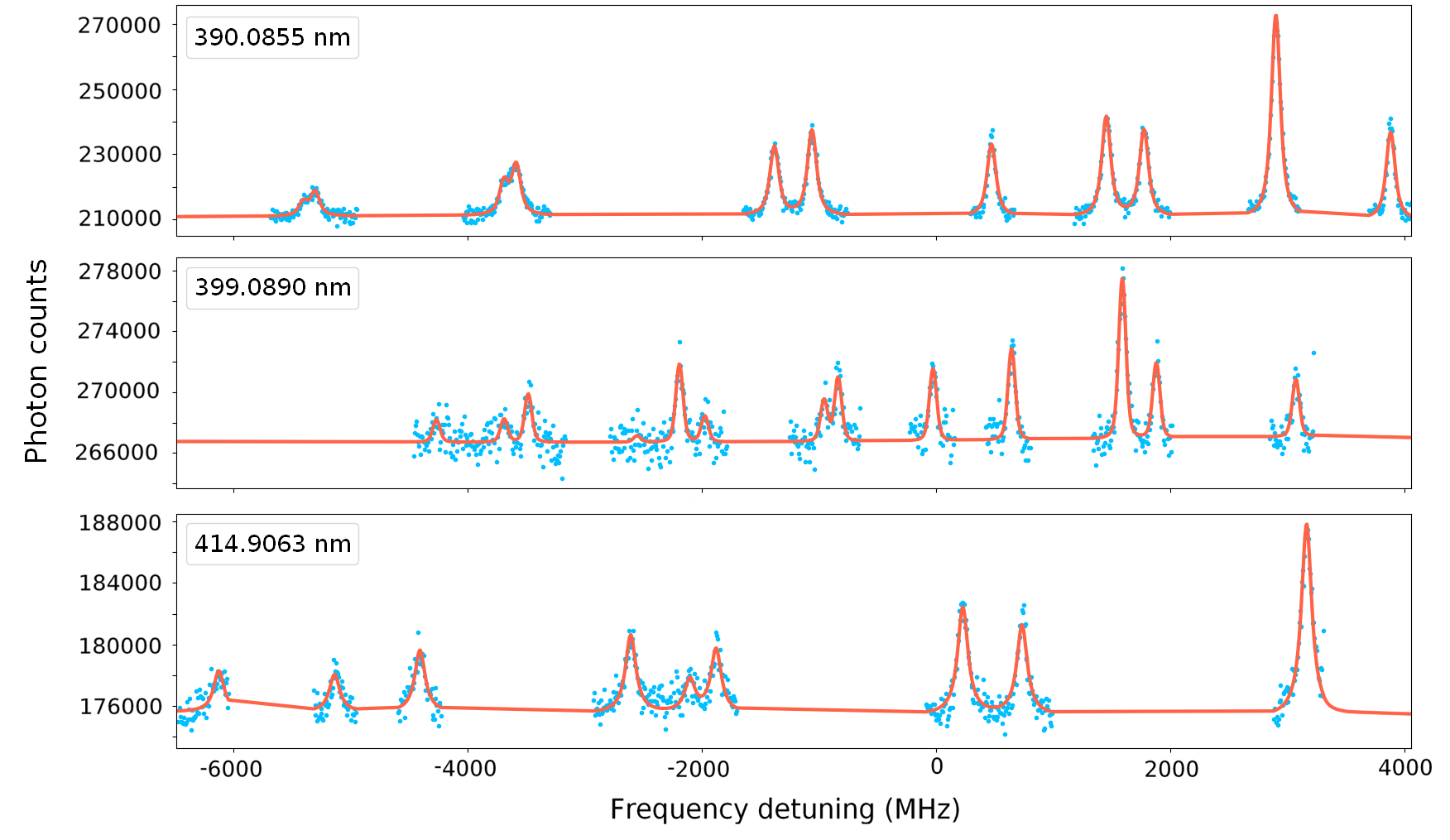
Spectroscopy was performed using three different optical transitions from the 3P state, as well as using one transition from the 4f146s2 1S0 ground state. These lines were the 399.0890 nm, 390.0855 nm and 414.9063 nm transitions (wavelengths in vacuum) to the 4f146p2 3P2, 4fF) 5d(2D)6s6p(3P∘) (2D) () and 4f146p2 3P1 states at 44760.370 cm-1, 45338.530 cm-1 and 43805.42 cm-1. The optical transition from the ground state is at 398.7986 nm, to the 4f146s6p 3D1 state at 25068.222 cm-1. After data processing, discussed in the next section, spectra similar to those shown in Fig. 2 are obtained for the different atomic lines. From our measurements we estimate the ratio of atoms in the 3P state to atoms in the 4f146s2 1S0 ground state is about 1:, in significant disagreement with the theoretical estimate Vernon et al. 2019. Despite this low number of metastable atoms, clear hyperfine structures can nevertheless be recorded in a few hours.
III.2 Analysis procedure
The measurement procedure outlined above yields the number of photon counts observed by the photomultipler tube (PMT) for every acceleration voltage in the sweep. Using this calibrated voltage, the laser frequency as observed in the rest frame of the atoms can be calculated via the relativistic Doppler shift formula:
| (8) | ||||
where is the sum of the cooler platform voltage and the acceleration voltage , and is the laser frequency as measured by the wavemeter. Hyperfine constants can then extracted from the obtained hyperfine spectra. For this, the SATLAS package Gins et al. 2018 was used. The spectra are fit by using Voigt profiles centered at the resonance locations predicted from Eqs. (1), corrected for second-order shifts given by Eq.(6).
Optimal values of the hyperfine constants, linewidths, peak heights and background are then obtained by performing a -minimization. Uncertainties are estimated from the inverse of the Hessian matrix, and are scaled with , where is obtained by dividing with the number of degrees of freedom. Each fit has seven free parameters related to the hyperfine structure constants (, and for each state, and furthermore a centroid wavelength). Since there are more than seven resonances for each of the transitions, the fit is over-determined, which helps to reduce the statistical uncertainties and to get precise values of the hyperfine coefficients, despite the somewhat poor signal-to-background for some scans.
The photon background was observed to vary over the scan range. The background is dominated by light spontaneously emitted by the ytterbium atoms following charge exchange. Scanning over large voltage ranges causes small changes in the atom trajectories, which changes the number of photons detected by the PMT. In order to fit this background, a second-order polynomial was used. Note that this choice of background shape affected the values of the hyperfine constants imperceptibly. For some of the spectra, partially overlapping resonances can be observed. The ratio of amplitudes of such overlapping peaks can be constrained to the ratio of the following theoretical intensities Campbell et al. 2016:
| (9) |
This helps to ensure convergence of the fit, and prevents convergence to nonphysically small amplitudes for one of the components.
III.3 Systematic Uncertainties
| A [MHz] | B [MHz] | C [MHz] | A [MHz] | B [MHz] | C [MHz] | |
|---|---|---|---|---|---|---|
| 399.0890 nm | -742.0(1) | 1347.2(10) | -0.01(7) | -123.4(10) | -629.8(9) | 0.08(7) |
| 390.0855 nm | -741.8(2) | 1348.9(19) | 0.12(13) | -347.6(2) | 120.0(18) | -0.15(14) |
| 414.9063 nm | -742.0(3) | 1345.4(23) | 0.01(17) | -0.01(45) | 484.0(12) | – |
| All lines | -741.98(9) | 1347.3(8) | 0.02(6) | – | – | – |
| 399.0890 nm (corr) | -742.0(1) | 1347.2(11) | -0.02(9) | -123.5(12) | -629.9(11) | 0.09(7) |
| 390.0855 nm (corr) | -741.8(2) | 1348.9(19) | 0.16(14) | -347.6(2) | 119.9(18) | -0.15(14) |
| 414.9063 nm (corr) | -742.0(3) | 1345.4(23) | 0.01(17) | -0.01(45) | 484.0(12) | – |
| All lines (corr) | -741.98(9) | 1347.3(9) | 0.03(7) | – | – | – |
| 769.9487 nm Singh et al. 2013 | -742.11(2) | 1339.2(2) | 0.54(2) | – | – | – |
One possible source of systematic uncertainty stems from the precision with which the ion beam energy can be determined.. Assuming an incorrect beam energy during the analysis will lead to a small stretching of the frequency scale of the hyperfine structure in the rest frame of the atoms, which in turn may skew the extracted hyperfine intervals. This is not expected to strongly influence the value of the hyperfine -constant, since the presence of a non-zero only manifests itself as a minor perturbation on top of the much larger dipole and quadrupole splittings. Nevertheless, care was taken to remove this potential systematic effect. This was done via a beam energy calibration using reference measurements of the accurately known hyperfine intervals of the ground state of singly-ionized 171,173Yb+ de Groote et al. 2020. In order to study the ionic ground state, after collecting several scans for each of the atomic transitions, the charge-exhange cell was brought to room temperature. The ion beam thus was no longer neutralized, and collinear laser spectroscopy was performed on the ionic 369.4192 nm line from 4f146s 2S1/2 to the 4f146p 2P state at 27061.82 cm-1. Three scans were taken for both 171,173Yb+. In the case of the present measurements, if the assumed beam energy is wrong by 10 eV, the extracted hyperfine intervals would be offset from literature values by about 2 MHz. By combining the three scans for 171Yb and 173Yb, we obtain a voltage offset of 34(5) V. This value was added to the total beam energy during the analysis. The systematic uncertainty on the hyperfine constants due to the 5 V uncertainty on the beam energy was also estimated and found to be negligible.
Care was also taken to optimize the mass resolving power of the dipole magnet, to make sure no 172,174Yb is present in the beam when studying 173Yb. Otherwise, if not accounted for, e.g. a small resonance of the even-even neighbours which lies close to a 173Yb resonance might affect the hyperfine constants. No evidence for resonances associated with these neighbouring masses (whose position is well known from separate measurements performed prior to measuring the structure of 173Yb) was seen in the spectra.
As will be shown in sectionIV, the data extracted for the three different transitions all yield consistent values. This provides a measure of confidence in the final hyperfine constants extracted here. It should be noted however that any source of systematic uncertainty which affects all three lines equally would remain undetected.
IV Results and discussion
IV.1 Hyperfine constants of the 3P-state

The hyperfine constants extracted from the measurements are summarized in Table 3. The numbers in round brackets are statistical and are calculated as the error on the weighted mean of the results for the individual scans of each transition. The fourth row and eighth row of the table show the weighted average of the three preceding rows. Values are presented with and without taking the second-order shifts discussed in section II.2 into account. The impact of the second-order shifts is rather small given our experimental uncertainties - the value of the hyperfine -constant shifts from 0.02(6) MHz to 0.03(7) MHz, but the average values of and do not change at the present precision. The hyperfine constants are also compared to literature. Good agreement with literature is obtained for the hyperfine coefficient, but the value of both and deviate. Interestingly, the hyperfine -constant of the 4f146p2 3P1 state is zero within our uncertainties.
The hyperfine -constant of the 3P state is zero within one standard deviation for every individual line. The weighted mean of the values of for this state from all 13 scans is 0.03(7) MHz (at the confidence level), which is significantly different from the value of 0.54(2) MHz obtained using the 769.9487 nm line Singh et al. 2013. This is shown graphically in the third panel of Fig. 3, which shows the values of and for every individual scan, as well as their weighted average. Fig. 3 serves to illustrate the excellent internal consistency of our dataset. Given that three different optical transitions were used to study the hyperfine structure of the 3P state, this provides confidence in our values of the hyperfine constants. The origins of the discrepancy between our value of and literature are unclear; further investigation using the 769.9487 nm transition in the future might help to resolve this puzzle. Currently, the wavelength of all light spontaneously emitted by the atom following the 769.9487 nm excitation lies outside of the wavelength sensitivity of our photo-multiplier tube, preventing us from making this measurement at the present time.
In order to extract a value of from our new value of for 173Yb, atomic structure calculations are required. The value of was reported as kHz/ in Singh et al. 2013. Using this value, we thus obtain -1.9(44) . From the calculations presented in this work (see Table 1), we find kHz/( b), yielding 6.7(160) .
IV.2 Discussion
The value of b obtained in Singh et al. 2013 was found to be many times larger than the simple shell model, which formed the motivation for the current work. An overview of the experimental values of available in the literature is given in Tab. 4, which serves to place into context the size of the value of of 173Yb obtained in Singh et al. 2013. An overview of the existing experimental values of , where is the mean-squared radius of the valence nucleon orbital, is furthermore shown in Fig. 4. Error bars represent the total uncertainties as reported in literature. To obtain values of , in principle theoretical calculations would be required, but as an approximation data on the total nuclear charge radius obtained from Angeli and Marinova 2013 were used. Fig. 4 also shows theoretical single-particle estimates of of a nucleus with spin containing an odd number of nucleons. These values can be calculated using Schwartz 1955
| (10) |
where for free protons and , for free neutrons. From the systematics of the magnetic dipole moments, it is well known that these free nucleon values do not provide an adequate description for the vast majority of nuclei. For this reason, often quenched values, usually , are adopted. This is also the approach we take here for the magnetic octupole moment.
Most values of lie between the curves predicted using Eq. (10), similar to the case for the magnetic dipole moments as well, with a few exceptions. As noted in Gerginov et al. 2003, the value for 133Cs is markedly larger than both the single-particle estimate without quenching, and even the quenched single-particle estimate is considerably smaller than the experimental value. Another example is reported for 155Gd Unsworth 1969, where is significantly larger than the quenched single-particle estimate (0.029 ) and the predictions by the strong coupling model (0.044 ) Williams 1962. However, the Gd atom has an opened and half-filled subshells. Thus, it poses a significant challenge for atomic-structure calculations to deal with the extremely complicated electron correlations and to achieve the required accuracy for extraction of from hyperfine splitting measurements.
From Fig. 4, it is clear that our new value of b is consistent with the simple shell model estimate. More precise measurements of are required in order to make more detailed comparisons with the shell model picture presented here, or with future large-scale nuclear structure calculations. For example, advanced large-scale shell model calculations are nowadays routinely used to accurately investigate the finer details of the magnetic dipole moments. For magnetic octupole moments such calculations would also be desirable, though so far only few attempts have been made Brown et al. 1980.
| Isotope | Z | N | State | [Hz] | Ref. | |
|---|---|---|---|---|---|---|
| 35Cl | 17 | 18 | 2P | -6.95(1.2) | -0.0188 | a |
| 37Cl | 17 | 20 | 2P | -5.41(1.2) | -0.0146 | a |
| 51V | 23 | 27 | 4D3/2 | -1660(140) | – | Childs et al. 1979 b |
| 23 | 27 | 4D5/2 | -270(80) | – | Childs et al. 1979 b | |
| 69Ga | 31 | 38 | 2P | 84(6) | 0.107(20) | Daly and Holloway 1954 |
| 71Ga | 31 | 40 | 2P | 115(7) | 0.146(20) | Daly and Holloway 1954 |
| 79Br | 35 | 44 | 2P | 388(8) | 0.116 | Brown and King 1966 |
| 81Br | 35 | 46 | 2P | 430(8) | 0.129 | Brown and King 1966 |
| 83Kr | 36 | 47 | 3P | -790(250) | -0.18(6) | Faust and Chow Chiu 1963 |
| 113In | 49 | 64 | 2P | 1728(45) | 0.565(12) | Eck and Kusch 1957 |
| 115In | 49 | 66 | 2P | 1702(35) | 0.574(15) | Eck and Kusch 1957 |
| 127I | 53 | 74 | 2P | 2450(370) | 0.167 | Jaccarino et al. 1954; Amoruso and Johnson 1971 |
| 131Xe | 54 | 77 | 3P | 728(105) | 0.048(12) | Faust and McDermott 1961 |
| 133Cs | 55 | 78 | 2P | 560(70) | 0.8(1) | Gerginov et al. 2003 |
| 137Ba | 56 | 81 | 2D3/2 | 36.546 | 0.05057(54) | Lewty et al. 2012 |
| 137Ba | 56 | 81 | 2D5/2 | -12.41(77) | 0.0496(37) | Lewty et al. 2013 |
| 151Eu | 63 | 88 | 8,10D | c | – | Childs 1991 |
| 153Eu | 63 | 90 | 8,10D | c | – | Childs 1991 |
| 155Gd | 64 | 91 | 3D | -1500(500) | -1.6(6) | Unsworth 1969 |
| 173Yb | 70 | 103 | 3P | 540(20) | -34.4(21) | Singh et al. 2013 |
| 175Lu | 71 | 104 | -617(57) | – | Brenner et al. 1985 | |
| 176Lu | 71 | 105 | -1377(302) | – | Brenner et al. 1985 | |
| 177Hf | 72 | 105 | 3F2 | 170(30) | – | Jin et al. 1995 |
| 72 | 105 | 3F3 | 230(90) | – | Jin et al. 1995 | |
| 72 | 105 | 3F4 | 500(190) | – | Jin et al. 1995 | |
| 179Hf | 72 | 107 | 3F2 | -410(50) | – | Jin et al. 1995 |
| 72 | 107 | 3F3 | -600(250) | – | Jin et al. 1995 | |
| 72 | 107 | 3F4 | -1190(500) | – | Jin et al. 1995 | |
| 197Au | 79 | 118 | 2D3/2 | 212(14) | 0.0098(7) | Blachman et al. 1967 |
| 79 | 118 | 4F | 326(10) | 0.130 | Blachman et al. 1967 | |
| 201Hg | 80 | 121 | 3P | -1840(90) | -0.130(13) | McDermott and Lichten 1960 |
| 209Bi | 83 | 126 | 2P | 19300(500) | 0.55(3)d | Landman and Lurio 1970 |
| 83 | 126 | 4S | 16500(100) | 0.43 | Hull and Brink 1970 | |
| 207Po | 84 | 123 | 3P2 | -12(1) | 0.11(1) | Olsmats et al. 1961; Fuller 1976 |
- a
J. H. Holloway, unpublished Ph.D. thesis, Department of Physics, MIT, 1956. Values taken from Brown and King 1966.
- b
Listing only significantly non-zero -values.
- c
Average ratio of -constants provided: C(151Eu)/C(153Eu) = 0.87(6).
- d
Value and uncertainty obtained as the average of several theoretical methods.
V Conclusion
We reported on the measurement of the hyperfine constants of the 3P state in neutral Yb. These measurements were performed using three different transitions with a standard collinear laser spectroscopy method, where the state of interest was populated through charge exchange with neutral potassium. From the data, we find that the hyperfine -constant is zero within experimental uncertainties. Our measurement thus resolves a puzzlingly large value reported in literature, which seemed difficult to reconcile with simple shell model estimates of the magnetic octupole moment. Future work to obtain the value of this magnetic octupole moment will require at least an order of magnitude improvement in precision. This could be achieved using e.g. a collinear laser-rf method, or another suitably high-precision technique. We also reported on a set of atomic structure caluclations of the second-order hyperfine shifts and the value of which will be required to interpret such future, higher-precision measurements.
Acknowledgements.
R.P.D.G. received funding from the European Union’s Horizon 2020 research and innovation programme under the Marie Skłodowska-Curie grant agreement No 844829. J.G.L. acknowledges the support of the National Natural Science Foundation of China under Grant No. 11874090.References
- Neyens (2003) G. Neyens, Reports on progress in physics 66, 633 (2003).
- Campbell et al. (2016) P. Campbell, I. Moore, and M. Pearson, Progress in Particle and Nuclear Physics 86, 127 (2016).
- Mertzimekis et al. (2016) T. Mertzimekis, K. Stamou, and A. Psaltis, Nuclear Instruments and Methods in Physics Research Section A: Accelerators, Spectrometers, Detectors and Associated Equipment 807, 56 (2016).
- Daly and Holloway (1954) R. T. Daly and J. H. Holloway, Phys. Rev. 96, 539 (1954).
- Jaccarino et al. (1954) V. Jaccarino, J. G. King, R. A. Satten, and H. H. Stroke, Phys. Rev. 94, 1798 (1954).
- Eck and Kusch (1957) T. G. Eck and P. Kusch, Phys. Rev. 106, 958 (1957).
- McDermott and Lichten (1960) M. N. McDermott and W. L. Lichten, Phys. Rev. 119, 134 (1960).
- Olsmats et al. (1961) C. Olsmats, S. Axensten, and G. Liljegren, Arkiv Fysik 19 (1961).
- Faust and McDermott (1961) W. L. Faust and M. N. McDermott, Phys. Rev. 123, 198 (1961).
- Faust and Chow Chiu (1963) W. L. Faust and L. Y. Chow Chiu, Phys. Rev. 129, 1214 (1963).
- Brown and King (1966) H. H. Brown and J. G. King, Phys. Rev. 142, 53 (1966).
- Blachman et al. (1967) A. G. Blachman, D. A. Landman, and A. Lurio, Phys. Rev. 161, 60 (1967).
- Unsworth (1969) P. J. Unsworth, Journal of Physics B: Atomic and Molecular Physics 2, 122 (1969).
- Hull and Brink (1970) R. J. Hull and G. O. Brink, Physical Review A 1, 685 (1970).
- Landman and Lurio (1970) D. A. Landman and A. Lurio, Phys. Rev. A 1, 1330 (1970).
- Childs et al. (1979) W. J. Childs, O. Poulsen, L. S. Goodman, and H. Crosswhite, Phys. Rev. A 19, 168 (1979).
- Brenner et al. (1985) T. Brenner, S. Büttgenbach, W. Rupprecht, and F. Träber, Nuclear Physics A 440, 407 (1985).
- Childs (1991) W. J. Childs, Phys. Rev. A 44, 1523 (1991).
- Jin et al. (1995) W. G. Jin, M. Wakasugi, T. T. Inamura, T. Murayama, T. Wakui, H. Katsuragawa, T. Ariga, T. Ishizuka, and I. Sugai, Phys. Rev. A 52, 157 (1995).
- Gerginov et al. (2003) V. Gerginov, A. Derevianko, and C. E. Tanner, Phys. Rev. Lett. 91, 072501 (2003).
- Lewty et al. (2012) N. C. Lewty, B. L. Chuah, R. Cazan, B. K. Sahoo, and M. D. Barrett, Opt. Express 20, 21379 (2012).
- Singh et al. (2013) A. K. Singh, D. Angom, and V. Natarajan, Phys. Rev. A 87, 012512 (2013).
- Xiao et al. (2020) D. Xiao, J. Li, W. C. Campbell, T. Dellaert, P. McMillin, A. Ransford, C. Roman, A. Derevianko, et al., Physical Review A 102, 022810 (2020).
- Brink and Satchler (1968) D. Brink and G. Satchler, “Angular momentum 2nd edn, clarendon,” (1968).
- Grant (2007) I. P. Grant, Relativistic Quantum Theory of Atoms and Molecules (Springer New York, 2007).
- Froese Fischer et al. (2016) C. Froese Fischer, M. Godefroid, T. Brage, P. Jönsson, and G. Gaigalas, Journal of Physics B: Atomic, Molecular and Optical Physics 49, 182004 (2016).
- Froese Fischer et al. (2019) C. Froese Fischer, G. Gaigalas, P. Jönsson, and J. Bieroń, Computer Physics Communications 237, 184 (2019).
- (28) J. Li, J. Ekman, G. Gediminas, J. Bieroń, P. Jönsson, M. Godefroid, and C. Froese Fischer, Computer Physics Communications (in preparation) .
- Jönsson et al. (1996) P. Jönsson, F. Parpia, and C. Froese Fischer, Computer Physics Communications 96, 301 (1996).
- Li et al. (2012) J. G. Li, P. Jönsson, M. Godefroid, C. Z. Dong, and G. Gaigalas, Physical Review A 86, 052523 (2012).
- Li et al. (2016) J. Li, M. Godefroid, and J. Wang, Journal of Physics B: Atomic, Molecular and Optical Physics 49, 115002 (2016).
- Porsev et al. (1999) S. Porsev, Y. G. Rakhlina, and M. Kozlov, Journal of Physics B: Atomic, Molecular and Optical Physics 32, 1113 (1999).
- Stone (2005) N. J. Stone, Atomic Data and Nuclear Data Tables 90, 75 (2005).
- Bohr and Weisskopf (1950) A. Bohr and V. F. Weisskopf, Phys. Rev. 77, 94 (1950).
- Kramida et al. (2019) A. Kramida, Y. Ralchenko, J. Reader, and NIST ASD TEAM, “NIST Atomic Spectra Database (version 5.7) [Online],” (2019).
- Vernon et al. (2019) A. Vernon, J. Billowes, C. Binnersley, M. Bissell, T. Cocolios, G. Farooq-Smith, K. Flanagan, R. G. Ruiz, W. Gins, R. de Groote, Á. Koszorús, K. Lynch, G. Neyens, C. Ricketts, K. Wendt, S. Wilkins, and X. Yang, Spectrochimica Acta Part B: Atomic Spectroscopy 153, 61 (2019).
- Vormawah et al. (2018) L. Vormawah, M. Vilén, R. Beerwerth, P. Campbell, B. Cheal, A. Dicker, T. Eronen, S. Fritzsche, S. Geldhof, A. Jokinen, et al., Physical Review A 97, 042504 (2018).
- Gins et al. (2018) W. Gins, R. P. de Groote, M. L. Bissell, C. G. Buitrago, R. Ferrer, K. M. Lynch, G. Neyens, and S. Sels, Comput. Phys. Comm. 222, 286 (2018).
- de Groote et al. (2020) R. de Groote, A. de Roubin, P. Campbell, B. Cheal, C. Devlin, T. Eronen, S. Geldhof, I. Moore, M. Reponen, S. Rinta-Antila, and M. Schuh, Nuclear Instruments and Methods in Physics Research Section B: Beam Interactions with Materials and Atoms 463, 437 (2020).
- Angeli and Marinova (2013) I. Angeli and K. Marinova, Atomic Data and Nuclear Data Tables 99, 69 (2013).
- Schwartz (1955) C. Schwartz, Phys. Rev. 97, 380 (1955).
- Williams (1962) S. A. Williams, Phys. Rev. 125, 340 (1962).
- Brown et al. (1980) B. A. Brown, W. Chung, and B. Wildenthal, Phys. Rev. C 22, 774 (1980).
- Amoruso and Johnson (1971) M. J. Amoruso and W. R. Johnson, Phys. Rev. A 3, 6 (1971).
- Lewty et al. (2013) N. C. Lewty, B. L. Chuah, R. Cazan, M. D. Barrett, and B. K. Sahoo, Phys. Rev. A 88, 012518 (2013).
- Fuller (1976) G. H. Fuller, Journal of Physical and Chemical Reference Data 5, 835 (1976).