Near-Optimal Design for Fault-Tolerant Systems with Homogeneous Components under Incomplete Information

In the design of control systems for industrial applications, it is important to achieve a certain level of fault tolerance. There has been a growing interest in the literature recently on developing effective fault tolerant paradigms for reliable control of real-world systems [1]. This type of control system is particularly useful when the system is subject to unpredictable failures. Recent applications of fault-tolerant control include power systems and aircraft flight control systems [2, 3].

It is known that certain class of faults can be modeled as partially observable Markov decision processes (POMDP). Various methods are studied in the literature to find an approximate solution to POMDP. Grid-based methods are used in [4] to compute an approximate value function at a fixed number of points in the belief space, and then interpolate over the entire space. The advantage of such approaches is that their computational complexity remains unchanged at each iteration and does not increase with time. Their drawback, however, is that the fixed points may not be reachable. In point-based methods [5], the reachability drawback is circumvented by restricting attention to the reachable set. Using the notion of $\alpha$-vectors, an approximate value function is obtained iteratively over a finite number of points in the reachable set. In these methods, the points are not fixed and may change with the value function. In policy-search methods such as finite-state controllers [6], on the other hand, attention is devoted to a certain class of strategies, and the objective is to find the best strategy in that class using policy iteration and gradient-based techniques. For more details on POMDP solvers, the interested reader is referred to [7, 5, 8], and references therein.

In this paper, a fault-tolerant scheme is proposed for a system consisting of a number of homogeneous components, where each component may fail with a certain probability. Three courses of action are defined to troubleshoot the faulty system: (i) let the system operate with faulty components; (ii) inspect the system, and (iii) repair the system. Each course of action has an implementation cost. The problem is formulated as a POMDP but since finding an optimal solution for this problem is intractable, in general, we are interested in seeking a near-optimal solution for it [9]. However, identifying an $\epsilon$-optimal solution for this problem is also NP-hard [10]. To overcome this hurdle, we exploit the structure of the problem to use a different information state (that is smaller than the belief state). The computational complexity of the proposed solution is logarithmic with respect to the desired neighborhood $\epsilon$, and polynomial with respect to the number of components. To derive some of the results, we use some methods developed in [11, 12].

This paper is organized as follows. The problem is formally stated in Section II and the main results of the work are presented in the form of three theorems in Section III. Two numerical examples are provided in Section IV and some concluding remarks are given in Section V.

Throughout this paper, $\mathbb{R}$ and $\mathbb{N}$ refer, respectively, to real and natural numbers. For any $n\in\mathbb{N}$, $\mathbb{N}_{n}$ denotes the finite set $\{1,\ldots,n\}$. Moreover, $\mathbb{P}(\bm{\cdot})$ is the probability of a random variable, $\mathbb{E}[\bm{\cdot}]$ is the expectation of a random variable, and $\mathbb{1}(\bm{\cdot})$ is the indicator function. The shorthand notation $x_{a:b}$ denotes vector $(x_{a},\ldots,x_{b})$, $a,b\in\mathbb{N},a\leq b$. For any finite set $\mathcal{X}$, $\mathcal{P}(\mathcal{X})$ denotes the space of probability measures on $\mathcal{X}$. For any $y,n\in\mathbb{N}$, $y\leq n$, and $p\in[0,1]$, $\Binopdf(y,n,p)$ is the Binomial probability distribution function of $y$ successful outcomes from $n$ trials where the success probability is $p$.

Consider a stochastic dynamic system consisting of $n\in\mathbb{N}$ internal components. Denote by $x^{i}_{t}\in\mathcal{X}:=\{0,1\}$ the state of component $i\in\mathbb{N}_{n}$ at time $t\in\mathbb{N}$, where $x^{i}_{t}=0$ means that the $i$-th component is in the operating mode and $x^{i}_{t}=1$ means that it is faulty. If a component is faulty, it remains so until it is repaired. Let $p\in[0,1]$ denote the probability that a component becomes faulty at any time $t\in\mathbb{N}$. It is assumed that the probability of failure of each component is independent of others.

Denote by $m_{t}=\sum_{i=1}^{n}x^{i}_{t}\in\mathcal{M}:=\{0,1,\ldots,n\}$ the number of faulty components at time $t\in\mathbb{N}$, and note that the state of each component may not be directly available. Let $o_{t}\in\mathcal{O}=\mathcal{M}\cup\{\mathtt{blank}\}$ denote the number of faulty components at time $t\in\mathbb{N}$ that are observed. If there is no observation at time $t\in\mathbb{N}$, then $o_{t}=\mathtt{blank}$. Initially, the system is assumed to have no faulty components, i.e. $o_{1}=0$.

At any time $t\in\mathbb{N}$, we have three different options (actions) at our disposal, represented by $u_{t}\in\mathcal{U}$, where $\mathcal{U}=\mathbb{N}_{3}$ is the action set. The first option is to do nothing and let the system continue operating without disruption at no implementation cost. In this case, no new information on the number of faulty components is collected, i.e.,

The second option is to inspect the system and detect the number of faulty components at some inspection cost, where

The third option is to repair the faulty components at a cost depending on the number of them, i.e. $m_{t}$. Therefore, at any time $t\in\mathbb{N}$, the following relations hold:

Let $c(m,u):\mathcal{M}\times\mathcal{U}\rightarrow\mathbb{R}$ denote the cost associated with action $u\in\mathcal{U}$ when the number of faulty components is $m\in\mathcal{M}$. The strategy $g$ is defined as the mapping from the available information by time $t$ to an action in $\mathcal{U}$, i.e.,

The objective is to develop a cost-efficient fault-tolerant strategy in the sense that the system operates with a relatively small number of faulty components, taking the inspection and repair costs into account. To this end, given the discount factor $\beta\in(0,1)$, we define the following cost:

To present the main result of this paper, we first derive a Bellman equation to identify the optimal solution. Since the corresponding Bellman equation involves an intractable optimization problem, we subsequently present an alternative Bellman equation that is tractable and provides a near-optimal solution. For any $m\in\mathcal{M}\backslash\{0,n\}$, define the following vector-valued function $\phi:\mathcal{M}\backslash\{0,n\}\rightarrow\mathcal{P}(0,1,.\ldots,n)$:

where $\ast$ denotes the convolution operator.

Let $s_{t}\in\mathcal{M}$ be the last observation before $t\in\mathbb{N}$ that is not blank and $z_{t}\in\mathbb{N}\cup\{0\}$ be the elapsed time associated with it, i.e., the time interval between the observation of $s_{t}$ and $t$.

For the sake of simplicity, denote by $T_{\scriptstyle\mathsf{m}}$ the transition probability matrix of the number of faulty components under actions $\{1,2\}$ given by Theorem 1, i.e., for any $m^{\prime},m\in\mathcal{M}$ and $t\in\mathbb{N}$,

Since the optimization of the Bellman equation (15) is carried out over a countable infinite set, it is computationally difficult to solve it. As a result, we are interested in a strategy which is sufficiently close to the optimal strategy and is tractable. To this end, define the following Bellman equation for any $k\in\mathbb{N}$, $s\in\mathcal{M}$ and $z\in\{0,1,\ldots,k\}$:

where

Let $c_{\text{max}}$ denote an upper bound on the per-step cost and $J^{\ast}$ denote the cost under the optimal strategy.

According to the strategy proposed in Theorem 3 (described by (18)), the near-optimal action at any time $t\in\mathbb{N}$ depends on the latest observation of the number of faulty components by that time ($s_{t}$) and the elapsed time since then $(z_{t})$. Note that the near-optimal action changes sequentially in time based on the dynamics of the state $(s_{t},z_{t})$, according to Lemma 1.

In this section, we aim to verify the main result presented in the preceding section by simulations. Consider a computing platform consisting of $n$ processors. Let $m_{t}$ denote the number of faulty processors at time $t\in\mathbb{N}$ and $p$ be the probability that a processor fails. The per-step cost under action $u_{t}=1$ is expressed as follows: $c(m_{t},1)=\ell(m_{t}),$ where $\ell(m_{t})\in\mathbb{R}_{\geq 0}$ is the cost of operating with $m_{t}$ faulty processors. The per-step cost under action $u_{t}=2$ is described as: $c(m_{t},2)=\ell(m_{t})+\alpha(m_{t}),$ where $\alpha(m_{t})\in\mathbb{R}_{\geq 0}$ is the cost of inspecting the system to detect the number of faulty processors. The per-step cost under action $u_{t}=3$ is formulated as: $c(m_{t},3)=\ell(m_{t})+\gamma(m_{t}),$ where $\gamma(m_{t})\in\mathbb{R}_{\geq 0}$ is the cost of repairing the faulty processors.

Example 1. Inspection and repair with fixed price. Let the cost of inspection and repair be constant, i.e., they do not depend on the number of faulty components. We consider the following numerical parameters:

Figure 1 shows the optimal course of action for the above setting, in different scenarios in terms of the number of faulty processors (based on the most recent observation). In this figure, the black color represents the first option (continue operating without disruption), gray color represents the second option (inspect the system and detect the number of faulty components) and the white color represents the third option (repair the faulty components). It is observed from the figure that that the inspection and repair options become more attractive as the number of faulty processors and/or the elapsed time since the last observation grow.

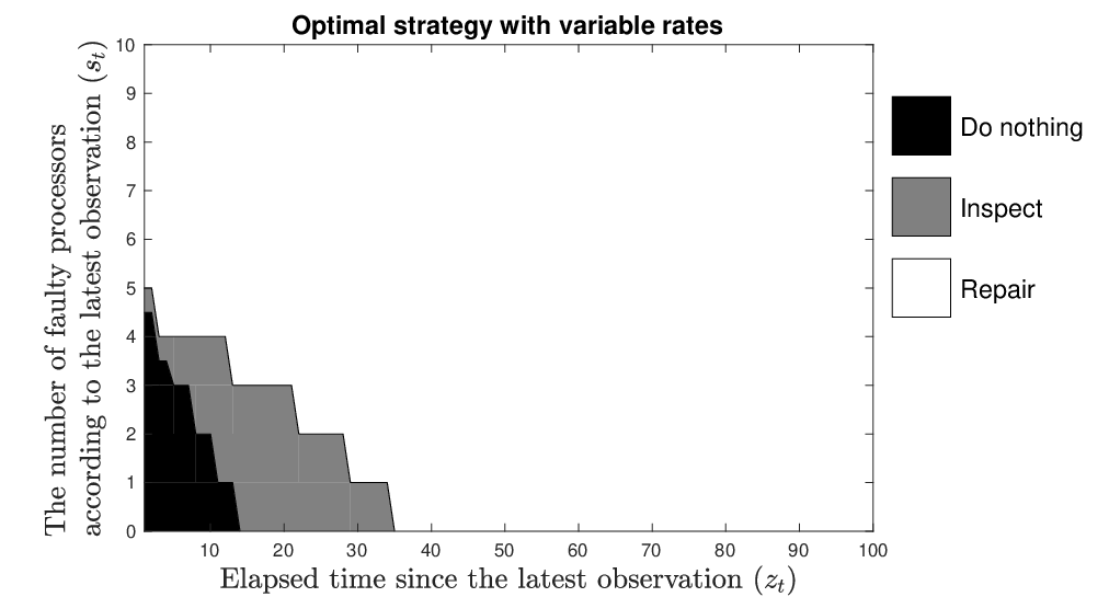
Example 2. Inspection and repair with variable price. Now, let the cost of inspection and repair be variable. We consider the same parameters as the previous example, except the following ones:

The results are presented in Figure 2, analogously to Figure 1. The figure shows that the inspection option is less desirable compared to Example 1, where the inspection and repair options prices were independent of the number of faulty processors. The reason is that with the variable rate, the repair option becomes more economical, hence more attractive than the previous case.

In this paper, we presented a fault-tolerant scheme for a system consisting of a number of homogeneous components, where each component can fail at any time with a prescribed probability. We proposed a near-optimal strategy to choose sequentially between three options: (1) do nothing and let the system operate with faulty components; (2) inspect to detect the number of faulty components, and (3) repair the faulty components. Each option incurs a cost that is incorporated in the overal cost function in the optimization problem. Two numerical examples are presented to demonstrate the results in the cases of fixed and variable rates. As a future work, one can investigate the case where there are a sufficiently large number of components using the law of large numbers [14].

References

- [1] P. M. Frank, “Trends in fault-tolerant control of engineering systems,” in Proceedings of the 11th IFAC Symposium on Automation in Mining, Mineral and Metal Processing, vol. 37, no. 15, pp. 377–384, 2004.
- [2] P. F. Odgaard, C. Aubrun, and Y. Majanne, “Fault tolerant control of power grids,” International Journal of Robust and Nonlinear Control, vol. 24, no. 8-9, pp. 1281–1282, 2014.
- [3] M. Verhaegen, S. Kanev, R. Hallouzi, C. Jones, J. Maciejowski, and H. Smail, Fault Tolerant Flight Control - A Survey. Berlin, Heidelberg: Springer Berlin Heidelberg, 2010, pp. 47–89.
- [4] W. S. Lovejoy, “Computationally feasible bounds for partially observed Markov decision processes,” Operations Research, vol. 39, no. 1, pp. 162–175, 1991.
- [5] G. Shani, J. Pineau, and R. Kaplow, “A survey of point-based POMDP solvers,” Autonomous Agents and Multi-Agent Systems, vol. 27, no. 1, pp. 1–51, 2013.
- [6] E. A. Hansen, “Finite-memory control of partially observable systems,” in Proceedings of the 14th Conference on Uncertainty in Artificial Intelligence, pp. 211–219, 1998.
- [7] A. R. Cassandra, “A survey of POMDP applications,” Working Notes of AAAI 1998 Fall Symposium on Planning with Partially Observable Markov Decision Processes, pp. 17–24, 1998.
- [8] K. P. Murphy, “A survey of POMDP solution techniques,” Technical report, U.C. Berkeley, 2000.
- [9] O. Madani, S. Hanks, and A. Condon, “On the undecidability of probabilistic planning and related stochastic optimization problems,” Artificial Intelligence, vol. 147, no. 1, pp. 5–34, 2003.
- [10] N. Meuleau, K.-E. Kim, L. P. Kaelbling, and A. R. Cassandra, “Solving POMDPs by searching the space of finite policies,” in Proceedings of the 15th Conference on Uncertainty in Artificial Intelligence, pp. 417–426, 1999.
- [11] J. Arabneydi and A. G. Aghdam, “Optimal dynamic pricing for binary demands in smart grids: A fair and privacy-preserving strategy,” in Proceedings of American Control Conference, 2018, pp. 5368–5373.
- [12] J. Arabneydi, “New concepts in team theory: Mean field teams and reinforcement learning,” Ph.D. dissertation, Department of Electrical and Computer Engineering, McGill University, Canada, 2016.
- [13] D. P. Bertsekas, Dynamic programming and optimal control. Athena Scientific, 4th Edition, 2012.
- [14] J. Arabneydi and A. G. Aghdam, “A certainty equivalence result in team-optimal control of mean-field coupled Markov chains,” in Proceedings of the 56th IEEE Conference on Decision and Control, 2017, pp. 3125–3130.