The variational method applied to the harmonic oscillator in presence of a delta function potential
Abstract
The problem of the harmonic oscillator with a centrally located delta function potential can be exactly solved in one dimension where the eigenfunctions are expressed as superpositions of the Hermite polynomials or as confluent hypergeometric functions in general. The eigenfunctions obtained exactly are difficult to visualise and hence to gain more insight, one can attempt using model wave functions which are explicitly and simply expressed. Here we apply the variational method to verify how close one can approach the exact ground state eigenvalues using such trial wave functions. We obtain the estimates of the ground state energies which are closer to the exact values in comparison to earlier approximate results for both the repulsive and attractive delta potentials.
I Introduction
The harmonic oscillator with the Hamiltonian,
| (1) |
is one of the most well known Hamiltonians in quantum mechanics that has been exactly solved in one and higher dimensions, the eigenfunctions here are expressed as product of a Gaussian function and the Hermite polynomials. The energy eigenvalues are with in one dimension. The solutions are of definite parity in all dimensions.
In this article we consider the harmonic oscillator (HO henceforth) in one dimension in presence of a centrally located delta function potential such that the Schrödinger equation obeyed by the eigenfunctions is
| (2) |
Here is the strength of the potential which is positive (negative) for a repulsive (attractive) potential. This problem can also be exactly solved. In presence of the delta function, the odd parity eigenfunctions are not affected. The energy for the even parity eigenfunctions can be obtained from a transcendental equation.
The delta function potential demands that there be a discontinuity in the first derivative of at the origin. Problems in quantum mechanics in presence of a delta function potential can be solved using a general prescription given in atkinson in one or higher dimensions. For the harmonic oscillator, the solution in Cartesian coordinates can be expressed as a superposition of the eigenstates of the HO, i.e., in terms of the Hermite polynomials.
Various methods have been used to obtain the eigenvalues for the harmonic oscillator in a delta function potential exactly atkinson; avakian; viana-gomes; ferkous or approximately patil. In viana-gomes, instead of taking the superposition of the eigenstates of the free HO, a different approach is used from which a lot of insight can be gained. The eigenfunctions are exactly identified in viana-gomes, however, these functions are not obtained in closed form and expressed implicitly in terms of integrals and are therefore not easy to visualise. An important question is therefore whether one can gain useful information by considering model wave functions which have explicit expressions and this approach was taken in patil. The expectation value of the energy was calculated using a model wave function and compared with the exact values.
Variational method is a well known approximation method griffiths used to estimate the upper bound of the ground state energy and in some cases higher level energies as well. Here a trial wave function is used which involves one or more parameters and their optimal values are obtained using the condition that is a minimum for these values. Variational method always overestimates the ground state energy since for any arbitrary trial wave function , where is the actual ground state energy.
In this article, we construct trial wave functions for the HO with a function potential, which obey some essential criteria (boundary conditions etc.) and use the variational method to obtain the optimal values of the parameters. Our aim is to see how close the actual ground state energy can be approached. We have used one parameter trial wave functions and obtained the results for the ground state energy which are in fact closer to the exact values compared to those in patil, where some model wave functions were used. We also discuss some extreme limits and basic features of the system using the present results.
II Exact result
In this section, we present the approach used in viana-gomes. The general solutions for the free harmonic oscillator (i.e., without the delta potential) can be expressed in terms of the confluent hypergeometric functions. The energy is written as and non-integer values are not allowed as that leads to some physical inconsistencies, discussed in detail in this section. For or a positive integer, the solutions are the well-known Hermite polynomials.
Changing the variables in equation (2) to dimensionless variables with , , , one gets the reduced Schrödinger equation
| (3) |
One can further use the notation as in viana-gomes. The solution for can be obtained in the form
| (4) |
The solutions for the differential equation obeyed by are expressed in terms of confluent hypergeometric functions known as Tricomi and Kummer functions arfken. Non-integer values of are not acceptable for for the following reasons: the Tricomi functions have a discontinuous derivative at the origin for non-integer and the Kummer functions, though smooth at the origin, blow up at infinity. However, these problems disappear for integer values of , in which case the Kummer and Tricomi functions reduce to the well known Hermite polynomials.
Now consider the effect of the delta function potential. For the odd solutions, the delta function potential is ineffective as the wave function is zero at the origin. However, the even parity solutions will be affected, and one requires a discontinuity in the first derivative in the wave function. Hence, in presence of the delta function potential, it is the Tricomi function with non-integer values of which is an appropriate solution having a discontinuity in the first derivative at the origin. But the Kummer functions are still not acceptable. Precisely, using the Tricomi function, the energy eigenvalues are obtained for by solving the transcendental equation
| (5) |
This equation has to be solved numerically to obtain the energy eigenvalues.
III Variational method for attractive delta


| Fig 2(a) | Fig 2(b) | Fig 2(c) | Fig 2(d) | ||||
|---|---|---|---|---|---|---|---|
| 0.10 | 0.7875843913490 | 0.855 | 0.15611114689438 | 0.86075 | 0.15608988843596 | 0.86094750 | 0.15608986490995 |
| 0.19 | 0.6330068382654 | 0.856 | 0.15610458365804 | 0.86080 | 0.15608987805867 | 0.86094763 | 0.15608986490987 |
| 0.28 | 0.4865632769097 | 0.857 | 0.15609922993587 | 0.86085 | 0.15608987067907 | 0.86094776 | 0.15608986490980 |
| 0.37 | 0.3714877335918 | 0.858 | 0.15609508353865 | 0.86090 | 0.15608986629690 | 0.86094789 | 0.15608986490976 |
| 0.46 | 0.2874437277571 | 0.859 | 0.15609214228512 | 0.86095 | 0.15608986491188 | 0.86094802 | 0.15608986490974 |
| 0.55 | 0.2288130659022 | 0.860 | 0.15609040400196 | 0.86100 | 0.15608986652375 | 0.86094815 | 0.15608986490973 |
| 0.64 | 0.1901599033527 | 0.861 | 0.15608986652375 | 0.86105 | 0.15608987113223 | 0.86094828 | 0.15608986490975 |
| 0.73 | 0.1672807821995 | 0.862 | 0.15609052769293 | 0.86110 | 0.15608987873706 | 0.86094841 | 0.15608986490979 |
| 0.82 | 0.1571204709131 | 0.863 | 0.15609238535979 | 0.86115 | 0.15608988933797 | 0.86094854 | 0.15608986490984 |
| 0.91 | 0.1574914723433 | 0.864 | 0.15609543738243 | 0.86120 | 0.15608990293470 | 0.86094867 | 0.15608986490992 |
For the attractive delta potential, .
We note that any trial wave function has to satisfy the following criteria
(a) It must have definite parity. Only the eigenvalues of even parity solutions will change due to the potential. The eigenvalues of the odd parity states will be identically ().
(b) It should vanish at infinity
(c) The first derivative for the even parity states must have a discontinuity at the origin obeying an equation given later in this section.
In accordance with the above criteria, we consider trial solutions in the form
| (6) |
for . Here is a normalisation constant depending on both and .
We note that the ground state of the harmonic oscillator should be recovered for such that and should be the optimal choice. On the other hand, for extremely large values of one expects the wave function to be dominantly of the form such that and . This indicates that the optimal values should follow the bounds: and with a sufficient condition at the extreme values. However, the discontinuity condition at the origin,
| (7) |
gives as a necessary condition when as given in equation (6) is used, which shows that cannot be taken as a variable. Here it may be mentioned that the model wave function that was considered in patil had an identical form with fixed values of the parameters; and . In our scheme we therefore keep only as variable and set henceforth and obtain the expectation value of the Hamiltonian which is expressed in terms of dimensionless parameter as

| From ref patil | ||||
|---|---|---|---|---|
| -5.0 | 0.219050 | -12.989190 | -12.990313 | -12.981750 |
| -3.0 | 0.362841 | -4.972539 | -4.972771 | -4.955630 |
| -2.5 | 0.426004 | -3.586291 | -3.5865066 | -3.565851 |
| -2.0 | 0.507489 | -2.442049 | -2.442360 | -2.418161 |
| -1.5 | 0.609289 | -1.532213 | -1.532729 | -1.506601 |
| -1.0 | 0.728909 | -0.841664 | -0.842418 | -0.819484 |
| -0.5 | 0.860948 | -0.343910 | -0.344424 | -0.333176 |
| 0.1 | 1.023871 | 0.054315 | 0.054269 | 0.054944 |
| 0.25 | 1.047595 | 0.128397 | 0.128106 | 0.131190 |
| 0.5 | 1.068158 | 0.234490 | 0.233519 | 0.241000 |
| 1.0 | 1.077488 | 0.394997 | 0.392743 | 0.404884 |
| 1.5 | 1.072723 | 0.506696 | 0.503881 | 0.516372 |
| 2.0 | 1.065157 | 0.586734 | 0.583894 | 0.595116 |
| 2.5 | 1.057843 | 0.645969 | 0.643356 | 0.652967 |
| 3.0 | 1.051491 | 0.691160 | 0.688831 | 0.696958 |
| 5.0 | 1.034671 | 0.797460 | 0.796119 | 0.800388 |

.
| (8) |
Therefore, with given by equation (6), the expectation value of the energy is given by (see Appendix A for details)
| (9) |
After expressing the integrals in terms of complementary error functions , we get
| (10) |
The aim is to find the value of that minimises . In principle one can differentiate with respect to and obtain the minimum value using a numerical method that locates the zero of the derivative. However, direct differentiation of in equation (III) to find the optimal value of leads to a complicated expression involving too many terms. Instead, we use a simple indirect method.
We explicitly evaluate for some specific values of and a window of values can be identified within which the minimum is located (indicative plots are given in figure 1 and 2 and the data corresponding to one value are tabulated in Table 1). Further evaluation of within this window is made and this process is continued till the desired accuracy up to six decimal places is reached, i.e., when the size of the window is less than .
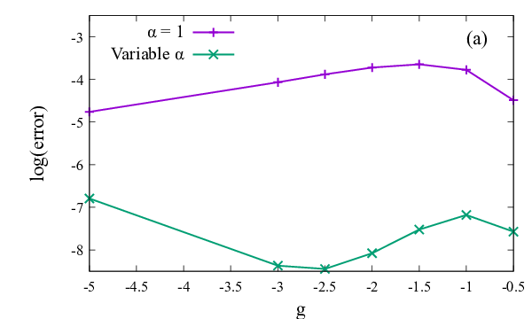
Both the absolute and relative errors compared to the exact values are shown in figure 3 and the results for are also shown for comparison. In Appendix B, the details of calculating numerically the exact values are given. It is indicated that the present method gives better results compared to the case . We have also plotted the optimal values in figure 4 and presented the values of and for some values of in Table 2. The inset of figure 4 shows that for large values of the attractive delta potential, indeed vanishes indicating the harmonic potential has little effect in that limit. We will come back to this point in the last section.


IV Variational principle for repulsive delta
The requirements for the trial wave function for repulsive delta potential are the same as that for the attractive one mentioned in the beginning of section III. We use the form of the trial wave function as
| (11) |
Once again, this form (used in patil with and ) satisfies the discontinuity condition (equation (7)) with specifically. In absence of the delta potential, the ground state wave function is therefore recovered and for very large values of , , the first excited state of a harmonic oscillator (apart from the absolute value of which is necessary for even parity). This is not surprising as an extremely strong delta potential will effectively break the system into two adjacent half-harmonic oscillators. We will discuss this in more detail in the next section.
We thus consider the variation of with respect to and set as in the attractive case. The expectation value of the energy using equation (11) is then given by
| (12) | |||
Variation of against shows the existence of a minimum as shown in figure 5 for specific values of . Here it is convenient to directly differentiate with respect to , and imposing the condition of minimum, we get
| (13) | |||
The optimal values of are obtained numerically using bisection method and the results for are presented in Table 2 along with the exact result and the result from patil. Also, we plot the deviations from the exact results in figure 6 that clearly show that the present results give better approximate values for . The optimal values of denoted by are plotted in figure 4.
V Discussions and Comparison with known results
In this paper, we have revisited the problem of the harmonic oscillator with a centrally located potential. Although the results are exactly known, it is useful to apply the variational principle of quantum mechanics to check how close one can approach the exact results and gain insight from the approximate solutions. We have dealt with the attractive and repulsive delta potential separately, using two different wave functions, taken in the form previously proposed in patil. We discuss here the behaviour of the approximate solutions in some limiting cases. In absence of the delta potential, the ground state wave function of the harmonic oscillator is of the form which means in equations (6) and (11). Hence for we expect . This is confirmed from the results for both attractive and repulsive potentials where indeed such a tendency is noted (figure 4).
In presence of an isolated attractive delta potential (i.e., when there is no harmonic potential), the wave function is of the form . In the limit we obtained using the variational method (figure 4) indicating the wave function is not affected by the presence of the HO potential. We present here an argument to support this result.
For the isolated attractive delta function there is a single bound state with energy
which is negative definite. Indeed, as increases in magnitude, this value is approached as shown in the numerical results (see Table 2; the data are also shown graphically in figure 7) and the corresponding . It is significant that for , has a negative value suggesting the delta function potential plays the dominant role. For , we thus argue following viana-gomes that the confining harmonic potential, too shallow compared to the delta potential, becomes irrelevant in the ground state. This implies one can treat the part of the Hamiltonian in equation (8) as a perturbation and is taken as the unperturbed Hamiltonian. The normalised unperturbed eigenfunction of is . The correction to the unperturbed energy eigenvalue from the first order perturbation theory would then be
| (14) |
For large values of the correction would therefore tend to vanish and the energy remains as . Also, there is only one bound state for the pure delta function potential (attractive). Hence, the correction to the wave function in the first order, , which has no overlap with this state is trivially zero. Thus one would expect to be the solution even in presence of the HO potential indicating in the variational method. Note that this argument is valid for the ground state, for the higher energy states, the confining potential will no longer be irrelevant. We also show in figure 7 that the limiting value is approached fairly rapidly using the variational method.
If , for the repulsive delta potential, we have, as mentioned earlier, effectively two disconnected half-harmonic oscillators on either side of the origin as the infinite potential barrier at the center is effectively insurmountable aouadi. In this limit, the ground state wave function is given by (as in figure 4). It is an interesting point that as , the value of approaches 1, an odd integer value (as shown in figure 7), giving rise to the so called anomalous degeneracy.

Now we get two different states belonging to the same eigenvalue (remember the odd parity state remains unaffected by the delta potential which is characterised by an odd integer value of ; here we are concerned with the state). This result may be apparently contradictory to the non-degeneracy theorem (and therefore the degeneracy is termed anomalous) in one-dimensional bound states in quantum mechanics. However, exceptions may occur as the proof of the non-degeneracy theorem rests on a few conditions. If any such condition does not hold good, e.g., if the product of the two supposedly degenerate wave functions is zero, non-degeneracy is not strictly imposed on the spectra of the system loudon. For the ground state, we have an understanding of the anomalous degeneracy from the present results. We take the two degenerate solutions as as given by the trial wave function for and , the first order excited state (exact). Then at the origin and albeit with different values of for and . This is consistent with the fact that if the product is zero, one can write in the regions where the product is non-zero but the constant may change discontinuously as one passes through a zero of . Non-uniqueness in the value of implies that the two functions are not trivially related and degeneracy will then exist. If is different on the two sides of the origin then the slopes of and cannot both be continuous at the origin, which is indeed the case here in presence of the delta function. Hence the anomalous degeneracy can exist here.
To summarise, the behaviour of the system is drastically affected in the limit of an extremely strong delta function, although differently for the attractive and repulsive case. In the attractive case, the wave function, peaking at the origin does not feel the effect of the harmonic potential () making as as the factor rapidly decreases with the increasing magnitude of . For the repulsive case on the other hand, as the wave function peaks away from the origin (occurs at ), the effect of the harmonic potential is stronger, such that is still close to unity. In fact remaining close to unity for the repulsive case for all values of may be understood using the same logic.
For intermediate values of for the attractive delta case, the value of obtained from the variational method shows significant deviation from 1, leading to appreciable changes in the energy values which are much closer to the exact values. In comparison, for the repulsive case, the energy values are closer to those obtained in patil as remains fairly close to unity even after applying the variational method.
One can ask the question, why does the variational method give ? The exact solution is of the form multiplied by the Tricomi function. The trial wave function, on the other hand, has multiplied by another function much simpler than the Tricomi function and does not contain , the parameter that is being varied. So the improvement in the result, that occurs through varying must lead to optimal value of as obtained from the variational method except at .
That the variational method works for the higher excited states can also be shown. We apply it for the known first excited state. The trial wave function for the first excited state has to be orthogonal to the trial wave functions in equation (6) and equation (11). Since any odd function will be orthogonal to these functions, a viable trial wave function is
| (15) |
The above wave function will do for both and . The energy expectation value is
| (16) |
Equation (16) is independent of which is physically consistent. So one might as well put which means we have the original HO states intact. This implies that one can put and in equation (16). Even if this is not done directly and both and is varied then from equation (16), we get a surface which is shown in Fig. 8. As we see the minima lies at irrespective of the value of . So, we can put in equation (16). Now the integrals convert into standard Gaussian integrals which can be easily performed. Explicit calculation shows the minimum occurs at . Hence one arrives at the exact result.
As an endnote, we mention that the problem of the harmonic oscillator has later been explored extensively introducing more intricacies like multiple delta functions in arbitrary positions and also in higher dimensions albeverio; aouadi; bush; ferkous; chua. It is also relevant for a charged particle in a magnetic field with a delta potential olega. The variational method should come in handy when we have to estimate the ground state energy of such cases. As we have shown without doing exact analysis we will be able to calculate accurate values of the energy by trial solutions. It can be a good pedagogical example for students to explore variational principle in a complicated problem and could be simpler in comparison to other variational methods like density matrix renormalisation group, also applied to quantum systems.
This problem has been dealt with in various other contexts also. For example, Bose condensation, which does not occur in one dimension, can happen so in presence of a point interaction localised at the origin papoyan. Similarly, the HO in a delta function potential in one dimension could be regarded as a possible model of the three-dimensional hydrogen molecular ion subjected to a static magnetic field in which the coulomb interactions are replaced by the corresponding one of simple point interactions. As the ionisation is relevant only along the direction of the field the three dimensional problem becomes a one dimensional one dunne; lapidus; lapidus2. In studying toponium, it was shown in avakian that HO with a point perturbation is a useful model to study quark interactions at short distances. However, such studies have been found to be unphysical later.

Acknowledgements: We are grateful to A, Raychaudhuri for discussions.
ORCID id: Parongama Sen : https://orcid.org/0000-0002-4641-022X
ORCID id: Indrajit Ghose : https://orcid.org/0000-0002-8561-4954
References
- (1) D. A. Atkinson, H. W. Crater, An exact treatment of the Dirac delta function potential in the Schrödinger equation, Am. J. Phys. 43 (1975) 301
- (2) M. P. Avakian, G. S. Pogosyan, A. N. Sissakian and V. M. Ter-Antonyan, Spectroscopy of a singular linear oscillator, Phys. Lett. A 124 (1987) 233
- (3) J. Viana-Gomes and N.M.R. Peres, Solution of the quantum harmonic oscillator plus a delta-function potential at the origin: the oddness of its even-parity solutions, Eur. J. Phys. 32 (2011) 1377
- (4) N. Ferkous, T. Boujedda, Bound states energies of a harmonic oscillator perturbed by point interactions, Commun. Theor. Phys. 67 (2017) 241
- (5) S. H. Patil, Eur. J. Phys., Harmonic oscillator with a -function potential, 27 (2006) 899
- (6) See e.g., D. J. Griffiths, Introduction to Quantum Mechanics, Pearson Education Limited, Delhi, 2014
- (7) G. B. Arfken, H. J. Weber and F. E. Harris, Mathematical Methods for Physicists, Academic Press, Walthum, 2013
- (8) O. Aouadi, Y. Chargui, and M. S. Fayache, J. Math. Phys. 57 (2016) 023522
- (9) R. Loudon, Am. J. Phys. 27 (1959) 649
- (10) T. Bush, B. G. Englert, K. Rzaewaski, M. Wilkens, Two Cold Atoms in a Harmonic Trap, Found. Phys. 28 (1998) 549
- (11) S. Albeverio, S. Fasari, F. Rinaldi, The Hamiltonian of the harmonic oscillator with an attractive -interaction centred at the origin as approximated by the one with a triple of attractive -interactions, J. Phys. A : Math. Theor. 49 (2016) 025302
- (12) C-K. Chua, Y-T. Liu and G-G. Wong, Time-independent Green’s function of a quantum simple harmonic oscillator system and solutions with additional generic delta-function potentials, J. Phys. Commun. 2 (2018) 035007
- (13) O. Olendski, One dimensional delta potentials in external fields, J. Phys. Cond. Matt, 7 (1995) 5607
- (14) V. V. Papoyan, V. A. Zagrebnov, On condensation of a one-dimensional nonideal Boson gas, Phys. Lett. A 113 (1985) 8
- (15) G. V. Dunne, C. S. Gauthier, Simple soluble molecular ionization model, Phys. Rev. A 69 (2004) 053409
- (16) I. R. Lapidus, One-Dimensional Model of a Diatomic Ion, Am. J. Phys. 38 (1970) 905
- (17) I. Richard Lapidus, One‐dimensional hydrogen molecule revisited, Am. J. Phys. 50 (1982) 453
- (18) M. Abramowitz and I. Stegun, Handbook of Mathematical Functions, Dover, New York, 1965
Appendix A
Here
| (17) |
Therefore
| (18) |
Substituting the expression of in equation (8) we get a term containing . We evaluate the term as follows
| (19) |
Simple algebra after this will lead to equation (9).
Appendix B
In solving the transcendental equation (equation (5)) we have evaluated the by using the defining property of a function.
| (B.20) | |||
| (B.21) |
where and is evaluated by equation (B.22).
The equation (6.1.35) from abramowitz gives
| (B.22) | |||
The values of are then calculated numerically using the bisection method.