跳到论文正文
W Papers独立论文阅读器 arXiv:2012.00347 论文正文 计算阅读时间 · 0%
引用这篇论文根据当前论文元数据生成,正式投稿前建议核对。


License: arXiv.org perpetual non-exclusive license
arXiv:2012.00347v1 [cs.IT] 01 Dec 2020

Signal Fractions Analysis and Safety-Distance Modeling in V2V Inter-lane Communications

Wenqiang Yi    Yuanwei Liu       Arumugam Nallanathan Thanks: W. Yi, Y. Liu, A. Nallanathan are with Queen Mary University of London, London E1 4NS, U.K. (email: {w.yi, yuanwei.liu, a.nallanathan}@qmul.ac.uk).
Abstract

For vehicular networks, safety distances are important, but existing spatial models fail to characterize this parameter, especially for inter-lane communications. This work proposes a Matérn hard-core processes based framework to appraise the performance of signal fractions (SF), where the hard-core distance is used to depict safety distances. By considering both semicircle and omnidirectional antennas, we derive high-accurate closed-form probability density functions of communication distances to acquire the complementary cumulative distribution function of SF. The derived expressions theoretically demonstrate that the nearest vehicle within the safety distance follows a uniform distribution and there is an upper limit for SF in terms of the transmit power.

Index Terms: 
Inter-lane V2V communications, Matérn hard-core process, signal fractions, stochastic geometry

I Introduction

With the rapid development of self-driving vehicles, in addition to sensing techniques, vehicle-to-vehicle (V2V) communications for transmitting instant instructions among vehicles become indispensable [1]. To evaluate the performance of large-scale V2V networks, practical spatial models are essential but challenging. Stochastic geometry is an efficient mathematical tool to model the locations of devices in wireless networks [2]. The authors in [3] illustrated that multiple 1D PPPs have the similar performance to 2D-PPP approaches. To characterize the safety distance between vehicles, the authors in [4] attempted Matérn hard-core processes (MHCP) to model the vehicles. For simplicity, the MHCP is regarded as a stationary thinning PPP. By utilizing a dynamic thinning PPP, the evaluation accuracy was improved in a recent work [5]. However, [5] omits a vital scenario, namely inter-lane communications, which is important for the lane-changing negotiation, intra-lane see-through ability, emergency/congestion broadcasting, etc. Such omission motivates this work.

Regarding evaluation metrics, existing performance-analysis works focus on coverage probabilities (outage probabilities) [1, 5, 4]. One main shortage of coverage probabilities is that the value range of the independent variable, namely the signal-to-interference-plus-noise ratio (SINR), is infinite. It is difficult to evaluate the overall trend of this metric, especially for numerical results. For V2V communications requiring ultra-high quality of services, the overall trend is a key factor for appraising technical designs since hidden drawbacks may be contained in the omitted value range. Therefore, this paper uses a new metric with a finite value range, namely signal fractions (SF) [6], which helps to show the complete information in a single numerical figure. Due to the finite value range, the integrals based on SF, e.g., the moments, do not turn to infinity. Note that the complementary cumulative distribution function (CCDF) of SF equals coverage probabilities but with different independent variables.

The main contributions of this work are: 1) We design a spatial model for intra-lane V2V communications based on multiple 1D MHCPs, where both the semicircle and omnidirectional antennas are considered; 2) Closed-form probability density functions (PDF) of the inter-lane communication distance are obtained; 3) A tractable CCDF of SF is provided based on a dynamic thinning PPP that has higher accuracy than the traditional method with a stationary thinning PPP.

II System Model

As shown in Fig. 1, a road with two 1D lanes is considered in this work, where vehicles in the ii-th lane (i∈{1,2})(i\in\{1,2\}) are modeled according to a 1D MHCP Φi⊂ℝ\Phi_{i}\subset\mathbb{R} with a hard-core distance did_{i} [2]. The generating PPP for all MHCPs is Φp\Phi_{p} with a density λp\lambda_{p}. A randomly selected typical vehicle in the first lane is fixed at the origin. Considering the distance between two lanes wlw_{l}, the 2D locations of all vehicles 𝕌v⊂ℝ2\mathbb{U}_{v}\subset\mathbb{R}^{2} is

𝕌v=⋃i=12⋃xi∈Φi{𝐮⁡(xi,(i−1)​wl)},\displaystyle\mathbb{U}_{v}=\bigcup\limits_{i=1}^{2}\bigcup\limits_{x_{i}\in\Phi_{i}}\{\mathbf{u}(x_{i},(i-1)w_{l})\}, (1)

where 𝐮⁡(x,y)\mathbf{u}(x,y) represents one point in the Cartesian coordinate system. Comparing with [5] that considers the range [0,∞)[0,\infty) for xx coordinates, this work assumes that x∈(−∞,∞)x\in(-\infty,\infty) to provide a general spatial model, which is vital for omnidirectional antennas. The definition of MHCP is provided as follows.

Definition 1.

(Matérn hard-core process): A type II MHCP Φh\Phi_{h} is generated from a generating PPP Φg\Phi_{g}. Given a mark m𝐱m_{\mathbf{x}}, which is uniformly distributed in [0,1][0,1], to each point 𝐱∈Φg\mathbf{x}\in\Phi_{g}, Φh\Phi_{h} retains the point 𝐱\mathbf{x} which obeys m𝐱>m𝐱′,∀𝐱′∈𝕊⁡(𝐱)∩Φgm_{\mathbf{x}}>m_{\mathbf{x}^{\prime}},\forall\mathbf{x}^{\prime}\in\mathbb{S}(\mathbf{x})\cap\Phi_{g}. The 𝕊⁡(𝐱)\mathbb{S}(\mathbf{x}) is the 1D ball centered at 𝐱\mathbf{x} with radius equalling to the hard-core distance.

From the definition, it worth noting that the distance between any two points in Φi\Phi_{i} is larger than did_{i}. Assuming the length of a vehicle is dvd_{v} and the safety distance between two vehicles is dsd_{s}11 1 The safety distance is decided by the speed of vehicles denoted by vsv_{s}. Following a two-second rule in driving, we have ds=2​vsd_{s}=2v_{s}., we define that di≡dv+dsd_{i}\equiv d_{v}+d_{s}. According to [5], the first order density of Φi\Phi_{i} is λi=1−exp⁡(−2​λp​di)2​di\lambda_{i}=\frac{1-\exp(-2\lambda_{p}d_{i})}{2d_{i}} and the corresponding second order density is

λi(2)​(r)\displaystyle{\lambda_{i}^{(2)}}(r) ={0,0<r≤di2​λir−2​(1−e−λp​(2​di+r))r⁡(2​di+r),di≤r<2​di.λi2,r≥2​di\displaystyle=\left\{{\begin{array}[]{*{20}{l}}{0,}&{0<r\leq{d_{i}}}\\ {\frac{2\lambda_{i}}{r}-\frac{2(1-e^{-\lambda_{p}(2d_{i}+r)})}{r(2d_{i}+r)},}&{{d_{i}}\leq r<2{d_{i}}}.\\ {\lambda_{i}^{2},}&{r\geq 2{d_{i}}}\\ \end{array}}\right.
Refer to caption
Fig. 1: Illustration of the spatial model for the considered V2V communications.

II-A Association Scheme

The V2V communication in the same lane has been investigated in [5]. This work considers another user association scheme: the nearest vehicle (NV) scheme, where the typical vehicle connects to the nearest vehicle in the adjacent lane.

For the NV scheme, the y-coordinate of the serving vehicle is yNV=wly_{\mathrm{NV}}=w_{l} and the x-coordinate can be expressed as

xNV=arg⁡minx2∈Φ2​|x2|.\displaystyle x_{\mathrm{NV}}=\arg\min\limits_{x_{2}\in\Phi_{2}}|x_{2}|. (5)

Therefore the location of the serving vehicle is 𝐮NV​(xNV,yNV)∈𝕌v\mathbf{u}_{\mathrm{NV}}(x_{\mathrm{NV}},y_{\mathrm{NV}})\in\mathbb{U}_{v}.

The condition (0<xNV≤d2)({0<x_{\mathrm{NV}}\leq{d_{2}}}) represents a practical scenario of lane changing. For example, when the in front serving vehicle wants to join to the typical vehicle’s lane, it checks the horizontal distance xNVx_{\mathrm{NV}} first. If the space between them is less than the safety distance, namely 0<xNV≤d2{0<x_{\mathrm{NV}}\leq{d_{2}}}, it needs to transmit its speed and acceleration to the typical vehicle to let the typical vehicle to do corresponding actions.

II-B Signal Model

We consider the metric SF instead of SINR. Since SINR is in a infinite range ℝ+\mathbb{R}^{+}, while SF is in a finite range, i.e., [0,1)[0,1), it is simpler to exploit the entire distribution of the SF. The definition of SF is [6]

Definition 2.

(Signal fraction): The SF is the ratio of the signal power SS to the total received power including interference II and noise NN, which can be expressed as

SF=ΔSS+I+N=SINRSINR+1.\displaystyle\mathrm{SF}\mathrel{\mathop{\kern 0.0pt=}\limits^{\Delta}}\frac{S}{S+I+N}=\frac{\mathrm{SINR}}{\mathrm{SINR}+1}. (6)

Based on Definition 2, the CCDF of SINR F¯SINR\bar{F}_{\mathrm{SINR}} can be calculated with the aid of the CCDF of SF F¯SF\bar{F}_{\mathrm{SF}}, i.e.,

F¯SF​(σ)=F¯SINR​(CLOSE​σ1−σ​).\displaystyle\bar{F}_{\mathrm{SF}}(\sigma)=\bar{F}_{\mathrm{SINR}}\hbox{$\left(\vbox to0.0pt{}\right.$}\frac{\sigma}{1-\sigma}\hbox{$\left)\vbox to0.0pt{}\right.$}. (7)

To enhance the generality, we consider two cases of antennas with unit antenna gain. Case 1: A semicircle antenna is deployed at the top of each vehicle. When transmitting, the antenna faces the behind, while the direction is changed to the front when receiving. Case 2: An omnidirectional antenna is used instead. After that, the SF can be expressed as

SFχ=|h𝐮NV|2​‖𝐮NV‖−α∑𝐮∈𝕌vχ|h𝐮|2​‖𝐮‖−α+ρ,\displaystyle\mathrm{SF}_{\chi}=\frac{|h_{\mathbf{u}_{\mathrm{NV}}}|^{2}\|\mathbf{u}_{\mathrm{NV}}\|^{-\alpha}}{\sum\limits_{\mathbf{u}\in\mathbb{U}^{\chi}_{v}}|h_{\mathbf{u}}|^{2}\|\mathbf{u}\|^{-\alpha}+\rho}, (8)

where χ∈{c1,c2}\chi\in\{c_{1},c_{2}\} is the case indicator and c1/c2c_{1}/c_{2} represents the Case 1/Case 2. The set 𝕌vc1=𝕌v|xi>0\mathbb{U}^{c_{1}}_{v}=\mathbb{U}_{v}|_{x_{i}>0} and 𝕌vc2=𝕌v\mathbb{U}^{c_{2}}_{v}=\mathbb{U}_{v}. The ρ=NPt​C\rho=\frac{N}{P_{t}C}, where PtP_{t} is the transmit power for all vehicles, CC is the free space path loss with a reference distance d0d_{0}, and α\alpha is the path loss exponent. The h𝐮h_{\mathbf{u}} represents the Rayleigh fading term for the link with the transmitter at 𝐮{\mathbf{u}}.

III Performance Evaluation

For light traffic, namely λp​di→0\lambda_{p}d_{i}\to 0, Φi≈Φp\Phi_{i}\approx\Phi_{p}, which is well-investigated in existing researches. Therefore, this work only discuss heavy traffic scenarios (λp​di≥1)(\lambda_{p}d_{i}\geq 1). Before analyzing the SF performance, we first derive the distribution of the distance between the typical vehicle and its serving vehicle.

III-A Distance Distributions

Under the NV scheme, the typical vehicle and the serving vehicle are respectively located in the first and second lane.

Lemma 1.

For the serving vehicle located in the adjacent lane, the PDF of the horizontal distance xNVx_{\mathrm{NV}} under Case 1 is

fxc1​(r1)≈{λ2,0<r1≤d2λ2​(1−λ2​(r1−d2)),d2<r1≤2​d2,λr​exp⁡(−λr​r1),r1>2​d2\displaystyle{f^{c_{1}}_{x}}\left({{r_{1}}}\right)\approx\left\{{\begin{array}[]{*{20}{l}}{{\lambda_{2}},}&{{0<r_{1}}\leq{d_{2}}}\\ {{\lambda_{2}}({1-{\lambda_{2}}({{r_{1}}-{d_{2}}})}),}&{{d_{2}}<{r_{1}}\leq 2{d_{2}}},\\ {{\lambda_{r}}\exp\left({-{\lambda_{r}}r_{1}}\right),}&{{r_{1}}>2{d_{2}}}\\ \end{array}}\right.

where λr=ln⁡(2(λ2​d2−2)2−2)/(2​d2)\lambda_{r}=\ln\left(\frac{2}{{{{\left({{\lambda_{2}}{d_{2}}-2}\right)}^{2}-2}}}\right)/(2d_{2}).

Proof:

See Appendix A. ∎

Remark 1.

From Lemma 1, it can be concluded that the distribution of xNVx_{\mathrm{NV}} in the range (0,d2](0,d_{2}] is a uniform distribution. Therefore, the PDF of the practical scenario of lane changing is fxc1​(r1|0<r1≤d2)=1/d2{f_{x}^{c_{1}}}\left({{r_{1}}}|{{0<r_{1}}\leq{d_{2}}}\right)=1/d_{2}.

For omnidirectional antennas, the serving and interfering vehicles can be either from the front or the back, namely xNVx_{\mathrm{NV}} can be smaller than zero. Under this case, we have the following corollary.

Corollary 1.

Base on Lemma 1, the PDF of the horizontal distance |xNV||x_{\mathrm{NV}}| under Case 2 is given by

fxc2​(r1)≈{2​λ2,0<r1≤d22g⁡(r1),d22<r1≤3​d222​λr​exp⁡(−λr​(2​r1+d))1−λ2​d2,r1>3​d22,\displaystyle{f^{c_{2}}_{x}}\left({{r_{1}}}\right)\approx\left\{{\begin{array}[]{*{20}{l}}{2{\lambda_{2}},}&{0<{r_{1}}\leq\frac{{{d_{2}}}}{2}}\\ {g\left({{r_{1}}}\right),}&{\frac{{{d_{2}}}}{2}<{r_{1}}\leq\frac{{3{d_{2}}}}{2}}\\ {\frac{{2{\lambda_{r}}\exp\left({-{\lambda_{r}}\left({2{r_{1}}+d}\right)}\right)}}{{1-{\lambda_{2}}{d_{2}}}},}&{{r_{1}}>\frac{{3{d_{2}}}}{2}}\\ \end{array}}\right.,

where g⁡(r1)=2​λ2​(1+λ2​d2/2−λ2​r1)1−λ2​d2​(CLOSE​3​λ2​d22−3​λ22​d228+e−2​λr​d2g(r_{1})=\frac{{2\lambda_{2}({1+{\lambda_{2}}{d_{2}}/2-{\lambda_{2}}{r_{1}}})}}{{1-{\lambda_{2}}{d_{2}}}}\hbox{$\left(\vbox to0.0pt{}\right.$}{\frac{{3{\lambda_{2}}{d_{2}}}}{2}-\frac{{3\lambda_{2}^{2}d_{2}^{2}}}{8}+e^{-2{\lambda_{r}}{d_{2}}}} −(CLOSE​λ2+λ22​d22​)​r1+λ22​r122​)-\hbox{$\left(\vbox to0.0pt{}\right.$}{{\lambda_{2}}+\frac{{\lambda_{2}^{2}{d_{2}}}}{2}}\hbox{$\left)\vbox to0.0pt{}\right.$}{r_{1}}+\frac{{\lambda_{2}^{2}r_{1}^{2}}}{2}\hbox{$\left)\vbox to0.0pt{}\right.$}.

Proof:

In this case, xNV∈(−∞,∞)x_{\mathrm{NV}}\in(-\infty,\infty). Based on fxc1​(r1){f^{c_{1}}_{x}}\left({{r_{1}}}\right), xNV∈[−d22,d22]x_{\mathrm{NV}}\in[-\frac{d_{2}}{2},\frac{d_{2}}{2}] is uniformly distributed with a density λ2\lambda_{2}. For xNV∈(−∞,−d22]∪[d22,∞)x_{\mathrm{NV}}\in(-\infty,-\frac{d_{2}}{2}]\cup[\frac{d_{2}}{2},\infty), we ignore the negligible correlation between the point process in (−∞,−d22](-\infty,-\frac{d_{2}}{2}] and [d22,∞)[\frac{d_{2}}{2},\infty). Note that the CDF of Y=min⁡(X1,X2)Y=\min(X_{1},X_{2}) is FY=Pr[min(X1,X2)<x]=1−(1−FX(x))2F_{Y}=\Pr[\min(X_{1},X_{2})<x]=1-(1-F_{X}(x))^{2}, where FXF_{X} is the CDF of X1X_{1} and X2X_{2}. After several algebraic manipulations, we obtain this corollary. ∎

Regarding the communication distance ‖𝐯NV‖\|\mathbf{v}_{\mathrm{NV}}\| between the serving vehicle and the typical vehicle, since the serving vehicle is in the second lane, the vertical distance is wlw_{l}. According the Pythagorean theorem, this distance is ‖𝐯NV‖=|xNV|2+wl2\|\mathbf{v}_{\mathrm{NV}}\|=\sqrt{|x_{\mathrm{NV}}|^{2}+w_{l}^{2}}.

Corollary 2.

Based on the NV scheme, the PDF of the communication distance ‖𝐯NV‖>wl\|\mathbf{v}_{\mathrm{NV}}\|>w_{l} can be expressed as follows

frχ​(r)=rr2−wl2​fxχ​(CLOSE​r2−wl2​),\displaystyle f^{\chi}_{r}(r)=\frac{r}{\sqrt{r^{2}-w_{l}^{2}}}f_{x}^{\chi}\hbox{$\left(\vbox to0.0pt{}\right.$}\sqrt{r^{2}-w_{l}^{2}}\hbox{$\left)\vbox to0.0pt{}\right.$}, (15)

where χ∈{c1,c2}\chi\in\{c_{1},c_{2}\} is the case indicator.

Proof:

The CDF of ‖𝐯NV‖\|\mathbf{v}_{\mathrm{NV}}\| is Frχ(r)=Pr[|xNV|2+wl2<r]=Pr[|xNV|2<r2−wl2]=Fxχ(r2−wl2)F^{\chi}_{r}(r)=\Pr[\sqrt{|x_{\mathrm{NV}}|^{2}+w_{l}^{2}}<r]=\Pr[|x_{\mathrm{NV}}|^{2}<\sqrt{r^{2}-w_{l}^{2}}]=F^{\chi}_{x}(\sqrt{r^{2}-w_{l}^{2}}). Based on frχ​(r)=d​Frχ​(r)d​r=d​Fxχ​(r2−wl2)d​rf^{\chi}_{r}(r)=\frac{dF^{\chi}_{r}(r)}{dr}=\frac{dF^{\chi}_{x}(\sqrt{r^{2}-w_{l}^{2}})}{dr}, we have this corollary. ∎

III-B Signal Fraction Performance

Given a target data rate RtR_{t}, the target SINR can be derived via Shannon-Hartley theorem, that is γt=2Rt/B−1\gamma_{t}=2^{R_{t}/B}-1, where BB is the system bandwidth. Before evaluating the performance of SF, we first derive the CCDF of SINR, namely the coverage probability, which is defined as

F¯SINRχ​(γt)=Pr⁡[​|h𝐮NV|2​‖𝐮NV‖−α∑𝐮∈𝕌vχ∖𝐮NV|h𝐮|2​‖𝐮‖−α+ρ>γt​]\displaystyle\bar{F}^{\chi}_{\mathrm{SINR}}(\gamma_{t})=\Pr\hbox{$\left[\vbox to0.0pt{}\right.$}\frac{|h_{\mathbf{u}_{\mathrm{NV}}}|^{2}\|\mathbf{u}_{\mathrm{NV}}\|^{-\alpha}}{\sum\limits_{\mathbf{u}\in{\mathbb{U}^{\chi}_{v}}\setminus{\mathbf{u}_{\mathrm{NV}}}}|h_{\mathbf{u}}|^{2}\|\mathbf{u}\|^{-\alpha}+\rho}>\gamma_{t}\hbox{$\left]\vbox to0.0pt{}\right.$} (16)
Theorem 1.

Under the NV scheme, the coverage probability for inter-lane communications between two adjacent lanes is

F¯SINRχ​(γt)≈∫wl∞exp⁡(−γt​(ρ+βχ​(I1+I2))​rα)​frχ​(r)​𝑑r,\displaystyle\bar{F}^{\chi}_{\mathrm{SINR}}(\gamma_{t})\approx\int_{w_{l}}^{\infty}{\exp({-{\gamma_{t}}({\rho+\beta_{\chi}({I_{1}}+{I_{2}}}))r^{\alpha}})}{f^{\chi}_{r}}({{r}})d{r}, (17)

where I1=λ1−1​∫d1∞λ1(2)​rd−α​d​rdI_{1}=\lambda_{1}^{-1}\int_{{d_{1}}}^{\infty}{\lambda_{1}^{\left(2\right)}}{r_{d}^{-\alpha}}dr_{d}, I2=∫0∞∫d2∞λ2(2)​(r)​fxc1​(r1)λ2​((r1+rd)2+wl2)α/2​d​rd​d​r1{I_{2}}=\int_{0}^{\infty}{\int_{{d_{2}}}^{\infty}{\frac{{\lambda_{2}^{(2)}\left(r\right){f^{c_{1}}_{x}}(r_{1})}}{{{{\lambda_{2}({{{({r_{1}+{{r_{d}}}})}^{2}}+w_{l}^{2}})}^{\alpha/2}}}}dr_{d}d{r_{1}}}}, βc1=1\beta_{c_{1}}=1, and βc2=2\beta_{c_{2}}=2.

Proof:

Since |h𝐮NV|2|h_{\mathbf{u}_{\mathrm{NV}}}|^{2} follows the exp⁡(1)\exp(1) distribution, (16) can be rewritten as

F¯SINRχ​(γt)=𝔼​[​exp⁡(CLOSE−γt​(CLOSE​∑𝐮∈𝕌vχ∖𝐮NV|h𝐮|2‖𝐮‖α+ρ​)​rα​)]\displaystyle\bar{F}^{\chi}_{\mathrm{SINR}}(\gamma_{t})=\mathbb{E}\hbox{$\left[\vbox to0.0pt{}\right.$}\exp\hbox{$\left(\vbox to0.0pt{}\right.$}-\gamma_{t}\hbox{$\left(\vbox to0.0pt{}\right.$}\sum\limits_{\mathbf{u}\in{\mathbb{U}^{\chi}_{v}}\setminus{\mathbf{u}_{\mathrm{NV}}}}\frac{|h_{\mathbf{u}}|^{2}}{\|\mathbf{u}\|^{\alpha}}+\rho\hbox{$\left)\vbox to0.0pt{}\right.$}r^{\alpha}\hbox{$\left)\vbox to0.0pt{}\right.$}\hbox{$\left]\vbox to0.0pt{}\right.$}
≈(a)∫wl∞e𝔼​[−γt​(CLOSE​∑𝐮∈𝕌vχ∖𝐮NV|h𝐮|2‖𝐮‖α+ρ​)​rα​]​frχ​(r)​𝑑r,\displaystyle\mathop{\approx}\limits^{(a)}\int_{w_{l}}^{\infty}e^{\mathbb{E}\hbox{$\left[\vbox to0.0pt{}\right.$}-\gamma_{t}\hbox{$\left(\vbox to0.0pt{}\right.$}\sum\limits_{\mathbf{u}\in{\mathbb{U}^{\chi}_{v}}\setminus{\mathbf{u}_{\mathrm{NV}}}}\frac{|h_{\mathbf{u}}|^{2}}{\|\mathbf{u}\|^{\alpha}}+\rho\hbox{$\left)\vbox to0.0pt{}\right.$}r^{\alpha}\hbox{$\left]\vbox to0.0pt{}\right.$}}f^{\chi}_{r}(r)dr, (18)

where (a)(a) uses Jensen’s inequality. For the interference under Case 2, we ignore the negligible correlation between the point distributed in (−∞,0)(-\infty,0) and (0,∞)(0,\infty), so βc2=2​βc1=2\beta_{c_{2}}=2\beta_{c_{1}}=2. By applying Campbell’s theorem [7] into (1), we obtain (17). ∎

Remark 2.

From Theorem 1, we find the coverage probability is inversely proportional to ρ\rho. The upper limit for F¯SINRχ\bar{F}^{\chi}_{\mathrm{SINR}} is F¯SINRχ|ρ=0\bar{F}^{\chi}_{\mathrm{SINR}}|_{\rho=0}.

It is worth noting that when γt\gamma_{t} is small, F¯SINRχ​(γt)\bar{F}^{\chi}_{\mathrm{SINR}}(\gamma_{t}) can be approximated by F1χ​(γt)=∫wl∞(1−γt​(ρ+βχ​(I1+I2))​rα)​frχ​(r)​𝑑rF^{\chi}_{1}(\gamma_{t})=\int_{w_{l}}^{\infty}{(1{-{\gamma_{t}}({\rho+\beta_{\chi}({I_{1}}+{I_{2}})})r^{\alpha}})}{f^{\chi}_{r}}({{r}})d{r} since limx→0exp⁡(−x)=1−x\lim\limits_{x\to 0}\exp(-x)=1-x. When γt\gamma_{t} is large, it can be approximated by F2χ​(γt)=λ2​∫wld22+wl2r​exp⁡(−γt​(ρ+βχ​(I1+I2))​rα)r2−wl2​𝑑rF^{\chi}_{2}(\gamma_{t})=\lambda_{2}\int_{w_{l}}^{\sqrt{d_{2}^{2}+w_{l}^{2}}}\frac{r\exp({-{\gamma_{t}}({\rho+\beta_{\chi}({I_{1}}+{I_{2}})})r^{\alpha}})}{\sqrt{r^{2}-w_{l}^{2}}}d{r} since the uniform-distribution part dominates F¯SINRχ​(γt)\bar{F}^{\chi}_{\mathrm{SINR}}(\gamma_{t}).

Corollary 3.

Based on the CCDF of SINR, the corresponding CCDF of SF is given by

F¯SFχ​(σ)≈∫wl∞exp⁡(CLOSE−σ⁡(ρ+I1+I2)​r1α1−σ​)​fxχ​(r1)​d​r1.\displaystyle\bar{F}^{\chi}_{\mathrm{SF}}(\sigma)\approx\int_{w_{l}}^{\infty}{\exp\hbox{$\left(\vbox to0.0pt{}\right.$}{-\frac{\sigma({\rho+{I_{1}}+{I_{2}}})r_{1}^{\alpha}}{1-\sigma}}\hbox{$\left)\vbox to0.0pt{}\right.$}}{f^{\chi}_{x}}(r_{1})d{r_{1}}. (19)
Proof:

By applying (7) to Theorem 1, we obtain this corollary. ∎

The F¯SFχ​(σ)\bar{F}^{\chi}_{\mathrm{SF}}(\sigma) has the same property as discussed in Remark 2. Moreover, F¯SFχ​(σ)\bar{F}^{\chi}_{\mathrm{SF}}(\sigma) can also be approximated using the same method as for F¯SINRχ​(γt)\bar{F}^{\chi}_{\mathrm{SINR}}(\gamma_{t}).

IV Numerical Result

As introduced in [6], we apply the Möbius homeomerphic (MH) unit to evaluate performance of SF, i.e., σ\sigma MH = σ1−σ\frac{\sigma}{1-\sigma}, (σ∈[0,1))(\sigma\in[0,1)). The network setting is listed as follows: C=λw216​π2​d02C=\frac{\lambda_{w}^{2}}{16\pi^{2}d_{0}^{2}}, the wavelength for 55 GHz is λw=3×10⁸/(5×109)=6\lambda_{w}=3\times 10^{8}/(5\times 10^{9})=6 cm, the reference distance d0=1d_{0}=1 m, α=4\alpha=4, N=−90N=-90 dBm, Pt=30P_{t}=30 dBm, λp=1/10\lambda_{p}=1/10 m-1, dv=5d_{v}=5 m, and wl=5w_{l}=5 m.

Refer to caption
Fig. 2: SF (Coverage probability) versus σ\sigma in MH (γt\gamma_{t}), with ds=145d_{s}=145 m and the comparison with a same density PPP [4].
Refer to caption
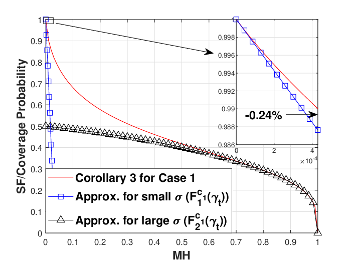
Fig. 3: Validating of approximation expressions, with λp=1/5\lambda_{p}=1/5 m-1 and ds=45d_{s}=45 m.
Refer to caption
Fig. 4: SF (Coverage probability) versus transmit power in W, with ds=95d_{s}=95 and σ=1/2\sigma=1/2 MH.

Fig. 2 shows the difference between the proposed method and the traditional method, which uses a replacement PPP with density λi\lambda_{i} to evaluate a MHCP [4]. Compared with the Monte Carlo simulations, the proposed CCDF of SF has a higher accuracy than the replacement PPP method, especially when α\alpha is small. Moreover, the omnidirectional antenna outperforms the semicircle antenna under the considered scenario. Note that when α\alpha is large, the near vehicles with short communication distance dominant the V2V network. Since the accuracy of the derived PDFs decreases with the increase of communication distances, our methods have higher accuracy in large α\alpha regimes than small α\alpha regimes. Fig. 2 also illustrates that SF explores the entire value range, i.e., [0,1)[0,1) with the finite independent variable σ∈[0,1)\sigma\in[0,1), while the independent variable for F¯SINRχ​(γt)\bar{F}^{\chi}_{\mathrm{SINR}}(\gamma_{t}) has an infinite value range, namely γt∈[0,inf)\gamma_{t}\in[0,\inf).

fxc1​(r1)=Pr⁡[​m𝐯>m𝐯′,𝐯∈Φp∩𝕃⁡(0,d2),𝐯′∈Φp∩𝕃⁡(r1−d2,r1+d2)∖𝐯​]\displaystyle{f^{c_{1}}_{x}}(r_{1})=\Pr\hbox{$\left[\vbox to0.0pt{}\right.$}m_{\mathbf{v}}>m_{\mathbf{v}^{\prime}},\mathbf{v}\in\Phi_{p}\cap\mathbb{L}(0,d_{2}),\mathbf{v}^{\prime}\in\Phi_{p}\cap\mathbb{L}\left(r_{1}-d_{2},r_{1}+d_{2}\right)\setminus\mathbf{v}\hbox{$\left]\vbox to0.0pt{}\right.$}
=(a)\displaystyle\mathop{=}\limits^{(a)} Pr⁡[​m𝐯>m𝐯1′,𝐯∈Φp∩𝕃⁡(0,d2),𝐯1′∈Φp∩𝕃⁡(0,d2)∖𝐯​]​Pr⁡[​m𝐯>m𝐯2′,𝐯2′∈Φp∩(𝕃⁡(r1−d2,0)∪𝕃⁡(d2,r1+d2))​]\displaystyle\Pr\hbox{$\left[\vbox to0.0pt{}\right.$}m_{\mathbf{v}}>m_{\mathbf{v}^{\prime}_{1}},\mathbf{v}\in\Phi_{p}\cap\mathbb{L}(0,d_{2}),\mathbf{v}^{\prime}_{1}\in\Phi_{p}\cap\mathbb{L}(0,d_{2})\setminus\mathbf{v}\hbox{$\left]\vbox to0.0pt{}\right.$}\Pr\hbox{$\left[\vbox to0.0pt{}\right.$}m_{\mathbf{v}}>m_{\mathbf{v}^{\prime}_{2}},\mathbf{v}^{\prime}_{2}\in\Phi_{p}\cap\left(\mathbb{L}(r_{1}-d_{2},0)\cup\mathbb{L}(d_{2},r_{1}+d_{2})\right)\hbox{$\left]\vbox to0.0pt{}\right.$}
=(b)\displaystyle\mathop{=}\limits^{(b)} ∑n=1∞(λp​d2)nn!​exp⁡(−λp​d2)​(n1)​1d2​∫01m𝐯n−1​exp⁡(−(1−m𝐯)​λp​d2)​d​m𝐯​=(c)1−exp⁡(−2​λp​d2)2​d2=λ2.\displaystyle\sum\limits_{n=1}^{\infty}{\frac{{{{\left({{\lambda_{p}}{d_{2}}}\right)}^{n}}}}{{n!}}\exp\left({-{\lambda_{p}}{d_{2}}}\right)}{n\choose 1}\frac{1}{{{d_{2}}}}\int_{0}^{1}{m_{\mathbf{v}}^{n-1}\exp\left({-\left({1-{m_{\mathbf{v}}}}\right){\lambda_{p}}{d_{2}}}\right)d{m_{\mathbf{v}}}}\mathop{=}\limits^{(c)}\frac{{1-\exp\left({-2{\lambda_{p}}{d_{2}}}\right)}}{{2{d_{2}}}}={\lambda_{2}}. (A.2)


Fig. 3 validates the approximation expressions for the CCDF of SF. We study Case 1 here as an example. When the value of σ\sigma is small, F¯SFc1​(σ)≈F1​(σ1−σ)\bar{F}^{c_{1}}_{\mathrm{SF}}(\sigma)\approx F_{1}\left(\frac{\sigma}{1-\sigma}\right). Under the considered condition, the approximation error for F¯SFc1​(σ)=F¯SINRc1​(γt)=99%\bar{F}^{c_{1}}_{\mathrm{SF}}(\sigma)=\bar{F}^{c_{1}}_{\mathrm{SINR}}(\gamma_{t})=99\% is around −0.24%-0.24\%. If unmanned vehicles require F¯SINRc1​(γt)≥99%\bar{F}^{c_{1}}_{\mathrm{SINR}}(\gamma_{t})\geq 99\%, namely the outage probability is less than 1%1\%, F1c1​(γt)F^{c_{1}}_{1}\left(\gamma_{t}\right) can be utilized for simplicity. On the other hand, when the value of σ\sigma is large, F¯SFc1​(σ)≈F2c1​(σ1−σ)\bar{F}^{c_{1}}_{\mathrm{SF}}(\sigma)\approx F^{c_{1}}_{2}\left(\frac{\sigma}{1-\sigma}\right).

Fig. 4 demonstrates the proposed insight. As discussed in Remark 2, Fig. 4 shows that F¯SFχ\bar{F}^{\chi}_{\mathrm{SF}} is proportional to the transmit power PtP_{t} and inversely proportional to the noise power for both cases. Moreover, Fig. 4 also illustrates that there is an upper limit of F¯SFχ\bar{F}^{\chi}_{\mathrm{SF}}, which means if the required coverage probability exceeds this upper limit, changing transmit power cannot satisfy the demand and hence additional interference cancellation methods are needed.

V Conclusion

This work has studied the SF performance for inter-lane V2V communications with the aid of MHCPs. Closed-form PDFs for communication distances have been provided. Based on these PDFs, the tractable CCDF of SF has been derived as well as several tight approximation expressions. Since there exists an upper limit of the SF performance, our future work will study interference cancellation techniques for dense V2V communications to break this limit.

Appendix A: Proof of Lemma 1

Under Case 1, we discuss the distribution of xNVx_{\mathrm{NV}} in three ranges: (0,d2](0,d_{2}], (d2,2​d2](d_{2},2d_{2}], and (2​d2,∞)(2d_{2},\infty).

V-1 0<xNV≤d20<x_{\mathrm{NV}}\leq d_{2}

The PDF of xNVx_{\mathrm{NV}} can be defined as

fxc1​(r1)\displaystyle~{f^{c_{1}}_{x}}(r_{1}) =Pr[Φ2∩𝕃(0,d2)=𝐯,𝐯∈Φp],\displaystyle=\Pr[\Phi_{2}\cap\mathbb{L}(0,d_{2})=\mathbf{v},\mathbf{v}\in\Phi_{p}], (A.1)

where 𝕃⁡(x1,x2)\mathbb{L}(x_{1},x_{2}) is the line segment from x1x_{1} to x2x_{2} in the second lane including the point at x2x_{2}. Based on the definition of MHCP, (A.1) can be rewritten at the top of this page.

In (IV), the process (a)(a) follows the fact that 𝕃⁡(r1−d2,r1+d2)=𝕃⁡(r1−d2,0)∪𝕃⁡(0,d2)∪𝕃⁡(d2,r1+d2)\mathbb{L}\left(r_{1}-d_{2},r_{1}+d_{2}\right)=\mathbb{L}\left(r_{1}-d_{2},0\right)\cup\mathbb{L}\left(0,d_{2}\right)\cup\mathbb{L}\left(d_{2},r_{1}+d_{2}\right). (b)(b) considers the void probability of PPPs and the similar process of (10) in [8]. (c)(c) uses the power series of exponential function, i.e., exp⁡(x)=∑n=0∞xnn!\exp(x)=\sum_{n=0}^{\infty}\frac{x^{n}}{n!}.

V-2 d2<xNV≤2​d2d_{2}<x_{\mathrm{NV}}\leq 2d_{2}

The PDF of xNVx_{\mathrm{NV}} can be defined as

fxc1​(r1)=\displaystyle{f^{c_{1}}_{x}}(r_{1})= Pr[Φ2∩𝕃(d2,2d2)=𝐯,𝐯∈Φp]\displaystyle\Pr[\Phi_{2}\cap\mathbb{L}(d_{2},2d_{2})=\mathbf{v},\mathbf{v}\in\Phi_{p}]
=\displaystyle= Pr⁡[​Φ2∩𝕃⁡(r1−d2,r1+d2)=𝐯⏟C1,\displaystyle\Pr\hbox{$\left[\vbox to0.0pt{}\right.$}\underbrace{\Phi_{2}\cap\mathbb{L}\left(r_{1}-d_{2},r_{1}+d_{2}\right)=\mathbf{v}}_{\mathrm{C_{1}}},
Φ2∩𝕃⁡(0,r1−d2)=∅⏟C2,𝐯∈Φp​]\displaystyle\ \ \ \ \ \underbrace{\Phi_{2}\cap\mathbb{L}(0,r_{1}-d_{2})=\emptyset}_{\mathrm{C_{2}}},\mathbf{v}\in\Phi_{p}\hbox{$\left]\vbox to0.0pt{}\right.$}
≈(d)\displaystyle\mathop{\approx}\limits^{(d)} λ2​(1−λ2​(r1−d2)),\displaystyle\lambda_{2}(1-\lambda_{2}(r_{1}-d_{2})), (A.3)

where (d)(d) ignores the overlapping between the conditions C1\mathrm{C_{1}} and C2\mathrm{C_{2}}. Assuming 𝐯1∈Φp∩𝕃⁡(0,r1−d2)\mathbf{v}_{1}\in\Phi_{p}\cap\mathbb{L}(0,r_{1}-d_{2}) and 𝐯2∈Φp∩𝕃⁡(r1−d2,r1)\mathbf{v}_{2}\in\Phi_{p}\cap\mathbb{L}(r_{1}-d_{2},r_{1}), this overlapping probability is

Po=\displaystyle P_{o}= Pr[m𝐯1<m𝐯2<m𝐯,|𝐯2−𝐯1|<d2]\displaystyle\Pr[m_{\mathbf{v}_{1}}<m_{\mathbf{v}_{2}}<m_{\mathbf{v}},|{\mathbf{v}_{2}}-{\mathbf{v}_{1}}|<d_{2}]
<\displaystyle< Pr[m𝐯1<m𝐯2<m𝐯]\displaystyle\Pr[m_{\mathbf{v}_{1}}<m_{\mathbf{v}_{2}}<m_{\mathbf{v}}]
=\displaystyle= ∫01exp⁡(−(1−m𝐯)​λp​d2)​d​m𝐯\displaystyle\int_{0}^{1}\exp\left(-(1-m_{\mathbf{v}})\lambda_{p}d_{2}\right)dm_{\mathbf{v}}
×∫0m𝐯exp⁡(−(1−m𝐯2)​λp​(r1−d2))​d​m𝐯2.\displaystyle\times\int_{0}^{m_{\mathbf{v}}}\exp\left(-(1-m_{\mathbf{v}_{2}})\lambda_{p}(r_{1}-d_{2})\right)dm_{\mathbf{v}_{2}}. (A.4)

Based on (V-2), when λp​d2\lambda_{p}d_{2} is large enough, we have limλp​d2→∞Po→0\lim\limits_{\lambda_{p}d_{2}\to\infty}P_{o}\to 0 and hence the overlapping is negligible.

V-3 xNV>2​d2x_{\mathrm{NV}}>2d_{2}

Under this case, xNVx_{\mathrm{NV}} can be divided into multiple segments with length d2d_{2} to calculate the PDF fxc1​(r1){f^{c_{1}}_{x}}(r_{1}). For each segment, the derivation has the similar proof process for the case (d2<r1≤2​d2)(d_{2}<r_{1}\leq 2d_{2}). However, this result delivers limited insights but with high complexity. Fortunately, when λp​d2≥1\lambda_{p}d_{2}\geq 1, the CDF of r1r_{1} in the range [0,2​d2][0,2d_{2}] is large enough:

FC​(2​d2)=λ2​d2+∫d22​d2λ2​(1−λ2​(r1−d2))​d​r1\displaystyle{F_{C}}(2d_{2})=\lambda_{2}d_{2}+\int_{d_{2}}^{2d_{2}}{\lambda_{2}\left({1-{\lambda_{2}}\left({{r_{1}}-{d_{2}}}\right)}\right)dr_{1}}
=\displaystyle= 2−(2−λ2​d2)22≥2−(3+exp⁡(−2))28≈0.77.\displaystyle 2-\frac{(2-\lambda_{2}d_{2})^{2}}{2}\geq 2-\frac{(3+\exp(-2))^{2}}{8}\approx 0.77. (A.5)

Therefore, we use a replacement 1D PPP with a density λr\lambda_{r} to approximate the PDF in the rest range, namely [2d2,+∞)[2d_{2},+\infty). The density λr\lambda_{r} obeys ∫2​d2∞λr​exp⁡(−λr​r)​𝑑r=1−FC​(2​d2)\int_{2d_{2}}^{\infty}\lambda_{r}\exp(-\lambda_{r}r)dr=1-{F_{C}}(2d_{2}). As a result, λr=ln⁡(CLOSE​2(λ2​d2−2)2−2​)/(2​d2)\lambda_{r}=\ln\hbox{$\left(\vbox to0.0pt{}\right.$}\frac{2}{{{{\left({{\lambda_{2}}{d_{2}}-2}\right)}^{2}-2}}}\hbox{$\left)\vbox to0.0pt{}\right.$}/(2d_{2}).

The proof is completed.

References

  • [1] A. Tassi, M. Egan, R. J. Piechocki, and A. Nix, “Modeling and design of millimeter-wave networks for highway vehicular communication,” IEEE Trans. Veh. Technol., vol. 66, no. 12, pp. 10 676–10 691, Dec. 2017.
  • [2] J. Illian, A. Penttinen, H. Stoyan, and D. Stoyan, Statistical analysis and modelling of spatial point patterns. John Wiley & Sons, 2008, vol. 70.
  • [3] M. J. Farooq, H. ElSawy, and M. Alouini, “A stochastic geometry model for multi-hop highway vehicular communication,” IEEE Trans. Wireless Commun., vol. 15, no. 3, pp. 2276–2291, Mar. 2016.
  • [4] F. J. Martin-Vega, B. Soret, M. C. Aguayo-Torres, I. Z. Kovacs, and G. Gomez, “Geolocation-based access for vehicular communications: Analysis and optimization via stochastic geometry,” IEEE Trans. Veh. Technol., vol. 67, no. 4, pp. 3069–3084, Apr. 2018.
  • [5] W. Yi, Y. Liu, Y. Deng, A. Nallanathan, and R. W. Heath, “Modeling and analysis of mmWave V2X networks with vehicular platoon systems,” IEEE J. Sel. Areas Commun., vol. 37, no. 12, pp. 2851–2866, Dec. 2019.
  • [6] M. Haenggi, “SIR analysis via signal fractions,” IEEE Commun. Lett., vol. 24, no. 7, pp. 1358–1362, Jul. 2020.
  • [7] D. J. Daley and D. Vere-Jones, An introduction to the theory of point processes: volume II: general theory and structure. Springer Science & Business Media, 2007.
  • [8] A. Al-Hourani, R. J. Evans, and S. Kandeepan, “Nearest neighbor distance distribution in hard-core point processes,” IEEE Commun. Lett., vol. 20, no. 9, pp. 1872–1875, Sep. 2016.