Single-particle digitization strategy for quantum computation
of a $\phi^{4}$ scalar field theory

Significant effort has been invested towards studying problems in quantum chemistry Whitfield et al. 2011; Kassal et al. 2011; O’Malley et al. 2016; Hempel et al. 2018, condensed matter physics Lewenstein et al. 2007; Bloch et al. 2012; Bao et al. 2015, cosmology Fischer and Schützhold 2004; Jain et al. 2007; Chatrchyan et al. 2020, and in high energy and nuclear physics Carlson et al. 2018; McCaskey et al. 2019; Dumitrescu et al. 2018; Rico et al. 2018; Cloët et al. 2019; Matchev et al. 2020, with digital quantum computers and analog quantum simulators Kielpinski et al. 2002; Monroe 2002; Blais et al. 2004; Cirac and Zoller 2012; Hauke et al. 2012; Preskill 2018. A major motivation is to deepen our understanding of conventionally intractable features of the ground state properties of strongly correlated many-body systems such as the spectrum of bound states. Another is to advance the state-of-the art in scattering problems, which provide dynamical information on such complex systems.

In this work, our focus will be on the problem of developing quantum algorithms for high energy scattering and multi-particle production in relativistic quantum field theory. Underlying our work is the promising yet distant goal of extracting dynamical information on the properties of hadrons and nuclei in quantum chromodynamics (QCD).

Examples of scattering problems in QCD where quantum information science can accelerate our present computational capabilities are low energy scattering in nuclear many-body systems  Roggero and Carlson 2018; Roggero et al. 2020, the thermalization process in ultrarelativistic ion-ion collisions Berges et al. 2020, studies of the structure of nuclear matter probed in Deeply Inelastic Scattering (DIS) of electrons off protons and nuclei Breidenbach et al. 1969; Bjorken 1969; Bjorken and Paschos 1969; Gross and Wilczek 1973; Blumlein 2013; Mueller et al. 2020; Lamm et al. 2020a; Kreshchuk et al. 2020a and the fragmentation of quarks and gluons into jets of hadrons Bassetto et al. 1983; Dokshitzer et al. 1988. For instance, both jet fragmentation functions and DIS structure functions require one to compute autocorrelation functions of currents in Minkowski spacetime; this poses a challenge to classical Monte Carlo methods that are constructed to compute Euclidean spacetime correlators Metz and Vossen 2016; Winter et al. 2017; Ji 2013; Alexandrou et al. 2015; Chen et al. 2016; Radyushkin 2017; Lin et al. 2018; Detmold et al. 2019.

Quantum devices have the potential to overcome the limitations of classical computers in addressing many of the above problems. However presently their limitation is that scattering problems involve a vast range of spatial (momentum) and temporal (energy) scales and require that a large number of (local) quantum field operators be quantum simulated. This is challenging with present day NISQ era technology restricted to few tens of non-error-corrected qubits Preskill 2018.

As discussed in seminal papers by Jordan, Lee and Preskill Jordan et al. 2011a; Jordan et al. 2012a, quantum simulating scattering problems in relativistic quantum field theories requires a lattice discretization and, in the case of a bosonic theory, the truncation of the local Hilbert space of field operators. One can view such a digitization as defining a low energy effective theory, in the sense of a generalized renormalization group (RG) Klco and Savage 2020. We will argue here that, from this viewpoint, a digitization scheme does not necessarily need to be based on a decomposition of local field operators but, more generally, should be based on the most economical implementation of the relevant directions of the RG for a specific problem.

Pursuant to this goal, we will explore a digitization strategy for the bosonic field theory of a real scalar field in $d+1$ spacetime dimensions based on a generalization of relativistic Bose-symmetrized “single particle states” previously discussed by us in Mueller et al. 2020. For a wide class of problems, this digitization requires resources that are only logarithmic in volume $\mathcal{V}$ (but linear in particle number), as opposed to field operator based approaches that depend linearly on the volume. We will discuss a strategy for initial state preparation, time evolution and measurement for scattering processes in high energy physics. Our time evolution algorithm has a gate complexity similar to that of Jordan et al. 2011a; Jordan et al. 2012a; however because the basis states are eigenstates of the free Hamiltonian and of the particle number operator, initial state preparation and measurement are particularly simple.

Our approach is unusual in the sense that relativistic many body systems are usually described by field operators within quantum field theory. In relativistic theories, particle number is not conserved and relativistic single particle states in position space are not Fourier conjugates of single particle states in momentum space. While it seems that these properties render quantum simulation of relativistic quantum field theory fundamentally different to those in quantum chemistry Whitfield et al. 2011; Kassal et al. 2011; O’Malley et al. 2016; Hempel et al. 2018 or in nonrelativistic low energy nuclear physics Carlson et al. 2018; McCaskey et al. 2019; Dumitrescu et al. 2018; Roggero and Carlson 2019, we will demonstrate here that this is not the case and that we are able to utilize algorithms that are conceptually similar.

A powerful motivation underlying our approach is the single particle picture Strassler 1992 behind the well known Feynman diagram techniques to compute scattering cross-sections in high energy physics at weak coupling. Because the computational complexity of Feynman diagram computations grows factorially with the required precision, their computation presents another opportunity for a quantum advantage Jordan et al. 2011a; Jordan et al. 2012a. Since as noted, scattering problems can be formulated in terms of Minkowski space field correlators, a first principles path integral computation with classical Monte Carlo techniques is challenging. Albeit considering a simpler theory, our ultimate aim is to apply this approach to quantum simulate scattering problems in quantum chromodynamics; a first step towards this goal would be a hybrid strategy combining a quantum treatment of some of the scattering degrees of freedom with a classical treatment of the rest Mueller et al. 2020. A relevant analogy in this regard is the simulation of quantum impurities in strongly correlated condensed matter systems Bauer et al. 2016, or the simulation of open quantum systems in heavy-ion collisions de Jong et al. 2020. In light of the many challenges of NISQ era computing, the digitization strategy we will present may therefore offer a useful compromise between being able to make progress in a limited class of problems in high energy physics with restricted resources and conceptual simplicity versus simulating any possible problem in quantum field theory in full generality.

This manuscript is organized as follows: In Section II, we will discuss the conceptual basis of our approach to quantum computing scattering cross-sections in high energy physics. Our digitization strategy is discussed in Section III. In Section IV, we will present the single particle digitization algorithm for quantum computing scattering cross-sections: state preparation is discussed in Section IV.1, the implementation of the time evolution operator as a quantum circuit in Section IV.2, the strategy to extract cross-sections through measurements in Section IV.3 and renormalization aspects of the problem in Section IV.4. In Section V, we summarize our results and discuss extensions of this approach to include theories with fermion and gauge fields with internal symmetries.

We elaborate on several of ths discussions in the main text in multiple appendices. In Appendix A, we provide details of the single particle digitization strategy. In Appendix B, we discuss the state preparation algorithm in greater detail. Appendices C, D and E contain details of the algorithm for the time evolution operator. Finally in Appendix F, we provide further details of the renormalization procedure.

Understanding the structure of matter at the sub-nucleon scales of nuclear and particle physics requires a wide range of scattering experiments. The theoretical foundations of these scattering problems is well developed within the framework of relativistic quantum field theory. The simplest formulation of a scattering process is through the S-matrix,

$\displaystyle S_{\beta\alpha}\equiv\langle\Psi^{\rm out}_{\beta}|\Psi^{\rm in}_{\alpha}\rangle\,,$

(1)

defined as the overlap of asymptotic in- ($|\Psi^{\rm in}_{\alpha}\rangle$) and out- ($|\Psi_{\beta}^{\rm out}\rangle$) states, that are time-independent eigenstates of the Hamiltonian $H=H_{0}+V$.

In the Heisenberg picture, all non-trivial information on these states is encoded in the Lippmann-Schwinger equation Lippmann and Schwinger 1950; Newton 2013,

$\displaystyle|\Psi_{\alpha}^{\rm in/out}\rangle=|\phi_{\alpha}\rangle+G_{0}V|\Psi_{\alpha}^{\rm in/out}\rangle=(V-VG_{0}V)^{-1}V|\phi_{\alpha}\rangle\,,$

where $|\phi_{\alpha}\rangle$ are single particle eigenstates of the free Hamiltonian $H_{0}$ satisfying $H_{0}|\phi_{\alpha}\rangle=E_{\alpha}|\phi_{\alpha}\rangle$, $G_{0}\equiv(E_{\alpha}-H_{0}\pm i\epsilon)^{-1}$ and $V-VG_{0}V$ is the Schwinger operator. The $S$-matrix can also be expressed as

$\displaystyle S_{\beta\alpha}=\delta_{\alpha\beta}-2\pi i\,\delta(E_{\alpha}-E_{\beta})\,T_{\beta\alpha}\,,$

(2)

where energy conservation is explicit, and the T-matrix is defined as

$\displaystyle T_{\beta\alpha}$

$\displaystyle=\langle\phi_{\beta}|V|\Psi^{\rm out}_{\alpha}\rangle=\langle\Psi^{\rm in}_{\beta}|V|\phi_{\alpha}\rangle=\langle\Psi^{\rm in}_{\beta}|(V-VG_{0}V)|\Psi^{\rm out}_{\alpha}\rangle\,.$

(3)

The cross-section for a scattering process $\alpha\rightarrow\beta$ is given by the modulus squared of $T_{\beta\alpha}$ (multiplied by kinematic factors),

$\displaystyle|T_{\beta\alpha}|^{2}=\langle\Psi^{\rm in}_{\alpha}|\,(V-VG_{0}V)P_{\beta}^{\rm out}(V-VG_{0}V)^{\dagger}\,|\Psi^{\rm in}_{\alpha}\rangle\,,$

(4)

with $P_{\beta}^{\rm out}=|\Psi^{\rm out}_{\beta}\rangle\langle\Psi^{\rm out}_{\beta}|$. The $T$-matrix elements in Eq. (3) can be computed by solving the Lippmann-Schwinger equation. This can be achieved using analytic perturbative techniques such as the Born expansion Newton 2013 or non-perturbatively using Schwinger’s variational principle Lippmann and Schwinger 1950, the Schwinger-Lanczos Meyer et al. 1991 or R-matrix approaches Wigner and Eisenbud 1947.

Quantum variants of these methods are currently under development; for an implementation of the Quantum-Lanczos algorithm in a scattering problem, see  Yeter-Aydeniz et al. 2020. We will proceed here with the formulation of the quantum scattering problem in the time-dependent Schrödinger picture Jordan et al. 2011b; Jordan et al. 2012b.

Before we proceed in that direction, we note that our single-particle digitization strategy for the S-matrix can be mapped on to a virial expansion, which is a ‘‘cluster” expansion in powers of the density that captures the many-body properties of a system at low particle densities. It is particularly successful in reproducing their ground state properties¹¹ 1 The extension of the virial expansion to non-equilibrium autocorrelation functions is highly non-trivial; an excellent review of this topic can be found in Dorfman et al. 1994; Dorfman et al.., which are expressed as a density expansion in the n-th order virial coefficients²² 2 This expression, originally formulated as a quantum many-body extension Huang and Yang 1957; Huang et al. 1957, to the famous Beth-Uhlenbeck formula was later generalized to discuss relativistic many-body $n\leftrightarrow m$ inelastic processes Dashen et al. 1969; Dashen and Rajaraman 1974.

$$b_{n}\propto\left[S^{\dagger}\frac{\partial S}{\partial E}\right]_{n}\,,$$

(5)

where $\left[S^{\dagger}\frac{\partial S}{\partial E}\right]_{n}$ of $n\rightarrow n$ scattering particles. Thus because our single particle strategy is optimal for capturing the many-body dynamics of a relativistic theory at low occupancies, a computation of $n\rightarrow n$ scattering matrix elements will allow us to determine ground state properties in our framework with the same range of validity as the virial expansion. Indeed, one can in principle go further and test the validity of this expansion relative to a direct computation of ground state properties of relativistic many-body systems in our framework.

In this Section, and in the next, we will develop a single particle digitization strategy for a relativistic (real) scalar field theory with local quartic interactions in $d+1$ spacetime dimensions. The Hamiltonian for this theory is given by

$\displaystyle{\bar{H}}=\int{\rm d}^{d}\textbf{x}\Big[\frac{\pi_{\mathbf{x}}^{2}}{2}+\frac{1}{2}(\nabla\phi_{\mathbf{x}})^{2}+\frac{\overline{m}^{2}}{2}\phi_{\mathbf{x}}^{2}+\frac{\overline{\lambda}}{4!}\phi^{4}_{\mathbf{x}}\Big]\,,$

(8)

where $\overline{m}$ and $\overline{\lambda}$ are the (bare) mass and quartic coupling, and $\nabla$ is the spatial gradient operator in $d$ dimensions. The Heisenberg field operators are

$\displaystyle\phi_{\mathbf{x}}=\int\frac{{\rm d}^{d}{\mathbf{p}}}{(2\pi)^{d}}\frac{1}{\sqrt{2\,\overline{\omega}_{\mathbf{p}}}}\Big[a_{\mathbf{p}}+a_{-{\mathbf{p}}}^{\dagger}\Big]e^{i{\mathbf{p}}\cdot\mathbf{x}}\,,$

(9)

which satisfies, with its canonical conjugate operator $\pi_{\mathbf{x}}$, the equal-time commutation relations $[\phi_{\mathbf{x}},\pi_{\mathbf{y}}]=i\delta^{(d)}(\mathbf{x}-\mathbf{y})$. The annihilation (creation) operators $a_{\mathbf{p}}$ ( $a^{\dagger}_{\mathbf{p}}$) are momentum-space Fock operators, corresponding to a set of harmonic oscillators with frequency $\overline{\omega}_{\mathbf{p}}=\sqrt{{\mathbf{p}}^{2}+\overline{m}^{2}}$ and commutation relations $[a_{\mathbf{p}},a^{\dagger}_{\mathbf{k}}]=(2\pi)^{d}\delta^{(d)}({\mathbf{p}}-\mathbf{k})$, $[a_{\mathbf{p}},a_{\mathbf{k}}]=[a^{\dagger}_{\mathbf{p}},a^{\dagger}_{\mathbf{k}}]=0$. Single particle states are defined as

$\displaystyle{|{\mathbf{p}}}\rangle^{\rm phys}\equiv\sqrt{2\,\overline{\omega}_{\mathbf{p}}}a^{\dagger}_{{\mathbf{p}}}|{\rm{vac}}\rangle\,,$

(10)

which satisfy the relativistic normalization condition $\langle{\mathbf{p}}|\mathbf{k}\rangle^{\rm phys}=2\,{\overline{\omega}}_{\mathbf{p}}\,\delta^{(3)}({\mathbf{p}}-\mathbf{k})$, where $|\rm vac\rangle$ denotes the Fock vacuum.

We discretize the theory on a spatial lattice of size $N_{s}^{d}$ and express the Hamiltonian (in dimensionless units) as

$\displaystyle H\equiv{a_{s}\bar{H}}=\sum_{\textbf{n}}\Big[\frac{1}{2}\pi^{2}_{\textbf{n}}+\frac{1}{2}({\nabla}\phi_{{\textbf{n}}})^{2}+\frac{{m}^{2}}{2}\phi^{2}_{\textbf{n}}+\frac{{\lambda}}{4!}\phi^{4}_{\textbf{n}}\Big]\,,$

(11)

where ${m}=\overline{m}\,a_{s}$, ${\lambda}=\overline{\lambda}\,a^{4-d}_{s}$ are dimensionless bare mass and coupling parameters, $a_{s}$ the lattice spacing and ${\textbf{n}}=(n_{1},\dots,n_{d})$, $n_{i}\in[0,N_{s}-1]$ labels a point $\mathbf{x}=\mathbf{n}a_{s}$ on the lattice. We will likewise define a momentum space lattice vector $\mathbf{q}=(q_{1},\dots,q_{d})$, $q_{i}\in[-\frac{N_{s}}{2},\frac{N_{s}}{2}-1]$. The lattice field operators are

	$\displaystyle\phi_{\mathbf{n}}=\frac{1}{\sqrt{\mathcal{V}}}\sum_{\mathbf{q}}\frac{1}{\sqrt{2{\omega}_{\mathbf{q}}}}\Big[a_{\mathbf{q}}+a^{\dagger}_{-\mathbf{q}}\Big]e^{i{2\pi}{}{\mathbf{n}\cdot\mathbf{q}}/N_{s}{}}\,,$
	$\displaystyle\pi_{\mathbf{n}}=\frac{-i}{\sqrt{\mathcal{V}}}\sum_{\mathbf{q}}\sqrt{\frac{\omega_{\mathbf{q}}}{2}}\Big[a_{\mathbf{q}}-a^{\dagger}_{-\mathbf{q}}\Big]e^{i{2\pi}{}{\mathbf{n}\cdot\mathbf{q}}/N_{s}{}}\,,$		(12)

where $\mathcal{V}=N_{s}^{d}$ and ${\omega}_{\mathbf{q}}=\overline{\omega}_{\mathbf{q}}\,a_{s}^{-1}$ is the dimensionless energy. Note that we use the same notation for the dimensionless lattice Fock operators $a_{\mathbf{q}}$ and the dimensionful continuum operators in Eq.(9).

We will implement below the time evolution operator of the free Hamiltonian (setting $\lambda=0$ in Eq.(11)) in the momentum representation. This allows us to use the continuum dispersion relation $\omega_{\mathbf{q}}=\sqrt{\mathbf{p}^{2}+m^{2}}$ ($\mathbf{p}\equiv\mathbf{p}(\mathbf{q})$), as opposed to the lattice dispersion relation that one has when working in position space; this potentially reduces discretization errors significantly.

The key idea in our digitization scheme is to decompose the many-particle Hilbert space into single particle sectors $\mathcal{H}=\bigotimes_{l=0}^{\infty}\mathcal{H}^{l}$, where a number of qubits are used to represent either momentum or position eigenstates in a binary decomposition. Since we are dealing with a relativistic theory where particle number is not conserved, an additional qubit is used to indicate whether or not a particle “exists”. With this in mind, the single particle Hilbert space is spanned by

$\displaystyle\mathcal{H}^{l}=\text{span}\{|\Omega\rangle^{(l)},\{|\mathbf{q}\rangle^{(l)}\}\}\,,$

(13)

where $\Omega$ denotes “empty states”, and $|\mathbf{q}\rangle$ “occupied states”. Further, a “register” of $N\equiv\log_{2}{\mathcal{V}}+1$ spins (qubits) represents a relativistic single-particle state with momentum $\mathbf{q}=(\textbf{q}_{1},\dots,\textbf{q}_{d})$ in $d$ dimensions,

$\displaystyle|\mathbf{q}\rangle^{(l)}\equiv\big|\textbf{q}_{1},\dots,\textbf{q}_{d}\rangle\big|\mathord{\uparrow}\big\rangle\,,$

(14)

where one qubit $|\mathfrak{n}\rangle=|\mathord{\uparrow}\rangle$ denotes that the single-particle state is occupied. Each momentum component of the occupied single-particle state

$\displaystyle|q_{i}\rangle\equiv|s_{i}\rangle||q_{i}|\rangle\,,$

(15)

is represented by $(N-1)/d$ qubits, where $s_{i}=\text{sign}(q_{i})$ is the sign (one qubit) and $|q_{i}|$ the absolute value (abs). Likewise, we define an unoccupied single-particle state as a state where abs, sign and occupation number qubits are all in the $|\downarrow\rangle$ state,

$\displaystyle|\Omega\rangle^{(l)}\equiv|\mathord{\downarrow}^{\otimes d\cdot N^{\rm abs}},\mathord{\downarrow}^{\otimes d},\mathord{\downarrow}\rangle\,,$

(16)

and the Fock vacuum is defined as $|{\rm vac}\rangle=\bigotimes_{l}|\Omega\rangle^{(l)}$. We will represent these momentum states using a binary encoding with the qubits representing the digits. In this case, $N^{\rm abs}=\frac{N-1}{d}-1=\frac{\log_{2}{(\mathcal{V}/2^{d})}}{d}$ qubits⁷⁷ 7 To avoid a sign ambiguity, we choose the lattice such that $q_{i}=0$ is excluded. Then $s_{i}=\mathord{\uparrow}$($\mathord{\downarrow}$) is a positive (negative) sign. We use a physical convention $|\mathord{\uparrow}/\mathord{\downarrow}\rangle$ of up/down spins to label states, instead of the more common $|0/1\rangle$ notation.. States with zero occupation number but finite $\mathbf{q}$ are unphysical and are excluded. Concrete examples of this single-particle digitization scheme are given in Appendix A. The normalization $\langle\mathbf{q}|\mathbf{q}^{\prime}\rangle=\delta_{\mathbf{q},\mathbf{q}^{\prime}}$ of these basis states differs from the relativistic normalization in Eq.(10), with $|\mathbf{q}\rangle=|{\mathbf{p}}\rangle^{\rm phys}/{\sqrt{2{\omega}_{\mathbf{q}}}}$. A generic state $|\psi\rangle^{(l)}\in\mathcal{H}^{l}$ can be written as

$\displaystyle|\psi\rangle^{(l)}=\mathfrak{a}_{0}|\Omega\rangle^{(l)}+\sum_{\mathbf{q}}\mathfrak{a}_{\mathbf{q}}|\mathbf{q}\rangle^{(l)}\,,$

(17)

with $|\mathfrak{a}_{0}|^{2}+\sum_{\mathbf{q}}|\mathfrak{a}_{\mathbf{q}}|^{2}=1$. The free part of the Hamiltonian ($H_{0}$) is block diagonal with the blocks labeled by the number of particles. Particle number eigenstates are on-shell single-particle states and those that are not correspond to virtual particles.

The Fock operators in Eq.(III) for the $M$ many-particle states on the combined Hilbert space $\mathcal{H}=\bigotimes_{l=0}^{\infty}\mathcal{H}^{l}$, are

$\displaystyle a_{\mathbf{q}}\equiv\lim_{M\rightarrow\infty}\frac{1}{\sqrt{M}}\sum_{l=0}^{M-1}a^{(l)}_{\mathbf{q}}\,,$

(18)

with $a^{(l)}_{\mathbf{q}},a^{(l)\dagger}_{\mathbf{q}}$ denoting chains of spin raising and lowering operators for each $\mathbf{q}$, and $(a^{(l)\dagger}_{\mathbf{q}})^{2}=(a^{(l)}_{\mathbf{q}})^{2}=0$. In practice, one truncates the number of single-particle registers at a finite $M$. If $M$ is large compared to the typical occupancy of a state $\mathfrak{n}\equiv\sum_{i}\mathfrak{n}^{(i)}$, the bosonic commutation algebra is realized, $[a_{\mathbf{q}},a^{\dagger}_{\mathbf{q}^{\prime}}]=\delta_{{\mathbf{q}},{\mathbf{q}}^{\prime}}+O(\frac{\mathfrak{n}}{M})$. Additional details of the construction are presented in Appendix A.

In the single-particle digitization of the Hilbert space of the scalar field theory, its dimension grows logarithmically with the volume $\mathcal{V}$ and linearly with $M$. This is ideal for high energy scattering problems, where the particle number density is small, such as the Bjorken limit Breidenbach et al. 1969; Bjorken 1969; Bjorken and Paschos 1969; Gross and Wilczek 1973 of the DIS problem we discussed earlier. The digitization is not economical for a very dense system because, as we will discuss, Bose symmetrization creates a large overhead of unphysical states. However, as we also noted, our digitization strategy could potentially be extended to such dense systems employing a hybrid quantum/classical approach.

In this Section, the single-particle digitization strategy will be formulated as a concrete algorithm to quantum compute scattering cross-sections. In line with the spacetime picture discussed in Section II, and paralleling the approach of Jordan, Lee and Preskill Jordan et al. 2011b; Jordan et al. 2012b, the components of our algorithm are

1. A.

   Initial state preparation, discussed in Section IV.1.

2. B.

   Simulating the time evolution, discussed in Section IV.2.

3. C.

   Measurement of observables and their relation to scattering cross-sections, discussed in Section IV.3.

4. D.

   Renormalization, discussed in Section IV.4.

These different elements are compactly summarized in Fig. (1).

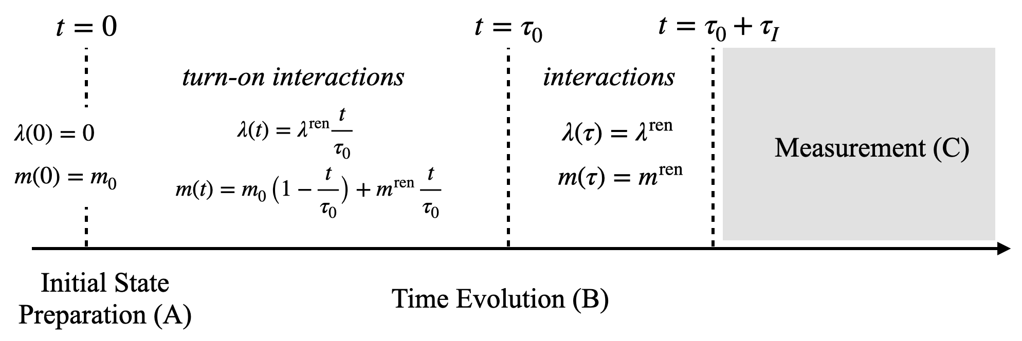
We will first discuss the preparation of the initial state of non-interacting particles in spatially separated wavepackets. Their preparation is particularly simple using the digitization presented in Section III compared to the field based approach of Jordan et al. 2011b; Jordan et al. 2012b; Klco and Savage 2019a, because single-particle states and the vacuum are computational basis states. Our algorithm consists of preparing a quantum mechanical superposition of these basis states to form wavepackets, placing them in separated regions of phase space and finally Bose-symmetrization of the resulting few/many-body wavefunction.

To implement the time evolution operator, we will employ a Suzuki-Trotter scheme⁸⁸ 8 For practical applications, it is important to note that more efficient algorithms for time evolution exist. One such example is the linear combination of unitaries Childs et al. 2017, later generalized to the method of quantum singular transformations Gilyén et al. 2019. The latter class of quantum algorithms not only significantly speeds up time evolution, but is also an efficient replacement of the classic phase estimation algorithm discussed in the context of measurements in Section IV.3. Trotter 1959; Suzuki 1976. We will treat the time evolution of the free and interacting parts of the Hamiltonian in Eq.(11) separately. We first evolve the wavepacket with the free Hamiltonian $H_{0}$, which is diagonal in the momentum representation. This is followed by a squeezing operation (analogous to that performed in quantum optics Gerry and Knight 2000; Yeter-Aydeniz and Siopsis 2018a), a quantum Fourier transformation Nielsen and Chuang 2010 from momentum space to position space, and lastly, an implementation of the interaction term in position space, where it is local.

This algorithm differs from the field based approach of Jordan et al. 2011b; Jordan et al. 2012b; Klco and Savage 2019a where the time evolution operator is split into a part diagonal in the $\phi_{\mathbf{x}}$-basis and one diagonal in the conjugate $\pi_{\mathbf{x}}$-basis. While the overall Trotter complexity scales as $O(\mathcal{V})$ in both cases, an important difference is that we avoid the lattice discretization of the Laplacian in Eq.(11) by working directly in momentum space.

Time evolution involves a switch-on of interactions from the non-interacting theory in the infinite past, $m(0)\equiv m_{0},\,\lambda(0)=0$ (in practice at some finite time $t=0$) towards acquiring the renormalized, physical couplings $m(\tau_{0})\equiv m^{\rm ren},\,\lambda(\tau_{0})=\lambda^{\rm ren}$ at $t=\tau_{0}$ right before the particles collide. The non-perturbative renormalization in the single-particle framework, which differs from that of Jordan et al. 2011b; Jordan et al. 2012b, is discussed in Section IV.4.

An important practical issue for the quantum algorithm is the spreading of the wavepackets during the switch-on time of interactions, which may potentially cause the wavepackets to interact before the coupling is turned to its final value. For this one may use the “forward-backward” evolution scheme outlined in Jordan et al. 2011b; Jordan et al. 2012b. Note however that because at large energies the dispersion is approximately linear $\omega\sim|\mathbf{p}|$, the spreading of the wavepackets is anticipated to be small Su et al. 1997.

Another relevant point is that the adiabatic preparation of single-particle states Jordan et al. 2011b; Jordan et al. 2012b will require a very large number of Trotter steps at high energies and likewise, for the turn-off of interactions. This can be understood by considering the energy gap between single-particle states with momentum $\mathbf{p}$ and energy $E=({\mathbf{p}^{2}+m^{2}})^{\frac{1}{2}}$, and the lowest of the two-particle states with total momentum $\tilde{\mathbf{p}}\equiv\mathbf{p}_{1}+\mathbf{p}_{2}$ (with relative momentum $\tilde{\mathbf{q}}\equiv\mathbf{p}_{1}-\mathbf{p}_{2}=0$) and energy $E=({\tilde{\textbf{p}}^{2}+(2m)^{2}})^{\frac{1}{2}}$ at weak coupling. Because this gap vanishes as $\mathbf{p}\rightarrow\infty$ and $\tilde{\mathbf{p}}\rightarrow\infty$, adiabatic state preparation is all but impractical at high energies.

Different state preparation algorithms have been suggested Lamm and Lawrence 2018; Kokail et al. 2019; Bapat and Jordan 2019; Harmalkar et al. 2020; Gustafson and Lamm 2020; Choi and Lee 2020 which are potentially faster than adiabatic state preparation. We note however that, departing from the strictly idealized S-matrix picture, in scattering processes such as Deeply Inelastic Scattering in QCD discussed in Section II.2, the Ioffe time and like physical scales are the relevant time scales for state preparation and may allow for quicker non-adiabatic state preparation. Because the algorithm discussed below is general, and one may also make use of alternative state preparation algorithms  Lamm and Lawrence 2018; Kokail et al. 2019; Bapat and Jordan 2019; Harmalkar et al. 2020; Gustafson and Lamm 2020; Choi and Lee 2020, we will not say anything further beyond noting this interesting possibility.

We will discuss finally in this Section the determination of scattering cross-sections, utilizing a natural connection of our digitization strategy to particle physics concepts. In contrast to field based digitizations Jordan et al. 2011b; Jordan et al. 2012b, particle number measurements do not require any additional gate operations. Measurement of energy density or momentum, for example, via a phase estimation algorithm, have a simple gate complexity. Some of the “classical analysis” in high energy experiments, of binning data or imposing kinematic cuts, can be incorporated directly in the quantum algorithm. We argue that, using novel techniques such as oblivious amplitude amplification Brassard et al. 2002; Nielsen and Chuang 2010; Berry et al. 2014, a quantum computer could possibly “beat” an actual particle physics experiment by producing rare events with a higher probability.

References

- Whitfield et al. (2011) J. D. Whitfield, J. Biamonte, and A. Aspuru-Guzik, Molecular Physics 109, 735 (2011).
- Kassal et al. (2011) I. Kassal, J. D. Whitfield, A. Perdomo-Ortiz, M.-H. Yung, and A. Aspuru-Guzik, Annual review of physical chemistry 62, 185 (2011).
- O’Malley et al. (2016) P. J. O’Malley, R. Babbush, I. D. Kivlichan, J. Romero, J. R. McClean, R. Barends, J. Kelly, P. Roushan, A. Tranter, N. Ding, et al., Physical Review X 6, 031007 (2016).
- Hempel et al. (2018) C. Hempel, C. Maier, J. Romero, J. McClean, T. Monz, H. Shen, P. Jurcevic, B. P. Lanyon, P. Love, R. Babbush, et al., Physical Review X 8, 031022 (2018).
- Lewenstein et al. (2007) M. Lewenstein, A. Sanpera, V. Ahufinger, B. Damski, A. Sen, and U. Sen, Advances in Physics 56, 243 (2007).
- Bloch et al. (2012) I. Bloch, J. Dalibard, and S. Nascimbene, Nature Physics 8, 267 (2012).
- Bao et al. (2015) N. Bao, P. Hayden, G. Salton, and N. Thomas, New Journal of Physics 17, 093028 (2015).
- Fischer and Schützhold (2004) U. R. Fischer and R. Schützhold, Physical Review A 70, 063615 (2004).
- Jain et al. (2007) P. Jain, S. Weinfurtner, M. Visser, and C. Gardiner, Physical Review A 76, 033616 (2007).
- Chatrchyan et al. (2020) A. Chatrchyan, K. Geier, M. K. Oberthaler, J. Berges, and P. Hauke, arXiv preprint arXiv:2008.02290 (2020).
- Carlson et al. (2018) J. Carlson, D. J. Dean, M. Hjorth-Jensen, D. Kaplan, J. Preskill, K. Roche, M. J. Savage, and M. Troyer, Quantum Computing for Theoretical Nuclear Physics, A White Paper prepared for the US Department of Energy, Office of Science, Office of Nuclear Physics, Tech. Rep. (USDOE Office of Science (SC)(United States), 2018).
- McCaskey et al. (2019) A. J. McCaskey, Z. P. Parks, J. Jakowski, S. V. Moore, T. D. Morris, T. S. Humble, and R. C. Pooser, npj Quantum Information 5, 1 (2019).
- Dumitrescu et al. (2018) E. F. Dumitrescu, A. J. McCaskey, G. Hagen, G. R. Jansen, T. D. Morris, T. Papenbrock, R. C. Pooser, D. J. Dean, and P. Lougovski, Physical review letters 120, 210501 (2018).
- Rico et al. (2018) E. Rico, M. Dalmonte, P. Zoller, D. Banerjee, M. Bögli, P. Stebler, and U.-J. Wiese, Annals of physics 393, 466 (2018).
- Cloët et al. (2019) I. C. Cloët, M. R. Dietrich, J. Arrington, A. Bazavov, M. Bishof, A. Freese, A. V. Gorshkov, A. Grassellino, K. Hafidi, Z. Jacob, et al., arXiv preprint arXiv:1903.05453 (2019).
- Matchev et al. (2020) K. Matchev, S. Mrenna, P. Shyamsundar, and J. Smolinsky, Quantum (2020).
- Kielpinski et al. (2002) D. Kielpinski, C. Monroe, and D. J. Wineland, Nature 417, 709 (2002).
- Monroe (2002) C. Monroe, Nature 416, 238 (2002).
- Blais et al. (2004) A. Blais, R.-S. Huang, A. Wallraff, S. M. Girvin, and R. J. Schoelkopf, Physical Review A 69, 062320 (2004).
- Cirac and Zoller (2012) J. I. Cirac and P. Zoller, Nature Physics 8, 264 (2012).
- Hauke et al. (2012) P. Hauke, F. M. Cucchietti, L. Tagliacozzo, I. Deutsch, and M. Lewenstein, Reports on Progress in Physics 75, 082401 (2012).
- Preskill (2018) J. Preskill, Quantum 2, 79 (2018).
- Roggero and Carlson (2018) A. Roggero and J. Carlson, arXiv preprint arXiv:1804.01505 (2018).
- Roggero et al. (2020) A. Roggero, A. C. Li, J. Carlson, R. Gupta, and G. N. Perdue, Physical Review D 101, 074038 (2020).
- Berges et al. (2020) J. Berges, M. P. Heller, A. Mazeliauskas, and R. Venugopalan, (2020), arXiv:2005.12299 [hep-th] .
- Breidenbach et al. (1969) M. Breidenbach, J. I. Friedman, H. W. Kendall, E. D. Bloom, D. H. Coward, H. C. DeStaebler, J. Drees, L. W. Mo, and R. E. Taylor, Phys. Rev. Lett. 23, 935 (1969).
- Bjorken (1969) J. D. Bjorken, Phys. Rev. 179, 1547 (1969).
- Bjorken and Paschos (1969) J. D. Bjorken and E. A. Paschos, Phys. Rev. 185, 1975 (1969).
- Gross and Wilczek (1973) D. J. Gross and F. Wilczek, Phys. Rev. Lett. 30, 1343 (1973), [,271(1973)].
- Blumlein (2013) J. Blumlein, Prog. Part. Nucl. Phys. 69, 28 (2013), arXiv:1208.6087 [hep-ph] .
- Mueller et al. (2020) N. Mueller, A. Tarasov, and R. Venugopalan, Physical Review D 102, 016007 (2020).
- Lamm et al. (2020a) H. Lamm, S. Lawrence, Y. Yamauchi, N. Collaboration, et al., Physical Review Research 2, 013272 (2020a).
- Kreshchuk et al. (2020a) M. Kreshchuk, W. M. Kirby, G. Goldstein, H. Beauchemin, and P. J. Love, arXiv preprint arXiv:2002.04016 (2020a).
- Bassetto et al. (1983) A. Bassetto, M. Ciafaloni, and G. Marchesini, Phys. Rept. 100, 201 (1983).
- Dokshitzer et al. (1988) Y. L. Dokshitzer, V. A. Khoze, S. Troian, and A. H. Mueller, Rev. Mod. Phys. 60, 373 (1988).
- Metz and Vossen (2016) A. Metz and A. Vossen, Prog. Part. Nucl. Phys. 91, 136 (2016), arXiv:1607.02521 [hep-ex] .
- Winter et al. (2017) F. Winter, W. Detmold, A. S. Gambhir, K. Orginos, M. J. Savage, P. E. Shanahan, and M. L. Wagman, Phys. Rev. D96, 094512 (2017), arXiv:1709.00395 [hep-lat] .
- Ji (2013) X. Ji, Phys. Rev. Lett. 110, 262002 (2013), arXiv:1305.1539 [hep-ph] .
- Alexandrou et al. (2015) C. Alexandrou, K. Cichy, V. Drach, E. Garcia-Ramos, K. Hadjiyiannakou, K. Jansen, F. Steffens, and C. Wiese, Phys. Rev. D92, 014502 (2015), arXiv:1504.07455 [hep-lat] .
- Chen et al. (2016) J.-W. Chen, S. D. Cohen, X. Ji, H.-W. Lin, and J.-H. Zhang, Nucl. Phys. B911, 246 (2016), arXiv:1603.06664 [hep-ph] .
- Radyushkin (2017) A. Radyushkin, Phys. Lett. B767, 314 (2017), arXiv:1612.05170 [hep-ph] .
- Lin et al. (2018) H.-W. Lin et al., Prog. Part. Nucl. Phys. 100, 107 (2018), arXiv:1711.07916 [hep-ph] .
- Detmold et al. (2019) W. Detmold, R. G. Edwards, J. J. Dudek, M. Engelhardt, H.-W. Lin, S. Meinel, K. Orginos, and P. Shanahan (USQCD), (2019), arXiv:1904.09512 [hep-lat] .
- Jordan et al. (2011a) S. P. Jordan, K. S. Lee, and J. Preskill, arXiv preprint arXiv:1112.4833 (2011a).
- Jordan et al. (2012a) S. P. Jordan, K. S. Lee, and J. Preskill, Science 336, 1130 (2012a).
- Klco and Savage (2020) N. Klco and M. J. Savage, arXiv preprint arXiv:2002.02018 (2020).
- Roggero and Carlson (2019) A. Roggero and J. Carlson, Physical Review C 100, 034610 (2019).
- Strassler (1992) M. J. Strassler, Nucl. Phys. B385, 145 (1992), arXiv:hep-ph/9205205 [hep-ph] .
- Bauer et al. (2016) B. Bauer, D. Wecker, A. J. Millis, M. B. Hastings, and M. Troyer, Phys. Rev. X 6, 031045 (2016).
- de Jong et al. (2020) W. A. de Jong, M. Metcalf, J. Mulligan, M. Płoskoń, F. Ringer, and X. Yao, (2020), arXiv:2010.03571 [hep-ph] .
- Lippmann and Schwinger (1950) B. A. Lippmann and J. Schwinger, Physical Review 79, 469 (1950).
- Newton (2013) R. G. Newton, Scattering theory of waves and particles (Springer Science & Business Media, 2013).
- Meyer et al. (1991) H.-D. Meyer, J. Horáek, and L. Cederbaum, Physical Review A 43, 3587 (1991).
- Wigner and Eisenbud (1947) E. P. Wigner and L. Eisenbud, Physical Review 72, 29 (1947).
- Yeter-Aydeniz et al. (2020) K. Yeter-Aydeniz, G. Siopsis, and R. C. Pooser, (2020), arXiv:2008.08763 [quant-ph] .
- Jordan et al. (2011b) S. P. Jordan, K. S. M. Lee, and J. Preskill, Quant. Inf. Comput.14,1014(2014) (2011b), arXiv:1112.4833 [hep-th] .
- Jordan et al. (2012b) S. P. Jordan, K. S. M. Lee, and J. Preskill, Science 336, 1130 (2012b), arXiv:1111.3633 [quant-ph] .
- Dorfman et al. (1994) J. Dorfman, T. R. Kirkpatrick, and J. V. Sengers, Annu. Rev. Phys. Chem. 45, 213 (1994).
- (59) J. Dorfman, T. R. Kirkpatrick, and J. V. Sengers, arXiv:1512.02679 [cond-mat.stat-mech] .
- Huang and Yang (1957) K. Huang and C. N. Yang, Phys. Rev. 105, 767 (1957).
- Huang et al. (1957) K. Huang, C. N. Yang, and J. M. Luttinger, Phys. Rev. 105, 776 (1957).
- Dashen et al. (1969) R. Dashen, S.-K. Ma, and H. J. Bernstein, Phys. Rev. 187, 345 (1969).
- Dashen and Rajaraman (1974) R. Dashen and R. Rajaraman, Phys. Rev. D 10, 708 (1974).
- Feynman (2018) R. P. Feynman, Photon-hadron interactions (CRC Press, 2018).
- Ioffe (1969) B. Ioffe, Phys. Lett. B 30, 123 (1969).
- Kovchegov and Strikman (2001) Y. V. Kovchegov and M. Strikman, Phys. Lett. B 516, 314 (2001), arXiv:hep-ph/0107015 .
- Wigner (1955) E. P. Wigner, Phys. Rev. 98, 145 (1955).
- Luscher (1986) M. Luscher, Commun. Math. Phys. 105, 153 (1986).
- Luscher (1991) M. Luscher, Nucl. Phys. B 354, 531 (1991).
- Hansen and Sharpe (2019) M. T. Hansen and S. R. Sharpe, Ann. Rev. Nucl. Part. Sci. 69, 65 (2019), arXiv:1901.00483 [hep-lat] .
- Briceno et al. (2018) R. A. Briceno, J. J. Dudek, and R. D. Young, Rev. Mod. Phys. 90, 025001 (2018), arXiv:1706.06223 [hep-lat] .
- Briceño et al. (2020) R. A. Briceño, J. V. Guerrero, M. T. Hansen, and A. Sturzu, (2020), arXiv:2007.01155 [hep-lat] .
- Brodsky et al. (1998) S. J. Brodsky, H.-C. Pauli, and S. S. Pinsky, Phys. Rept. 301, 299 (1998), arXiv:hep-ph/9705477 .
- Susskind (1968) L. Susskind, Phys. Rev. 165, 1535 (1968).
- Bjorken et al. (1971) J. Bjorken, J. B. Kogut, and D. E. Soper, Phys. Rev. D 3, 1382 (1971).
- Weinberg (1967) S. Weinberg, Phys. Rev. Lett. 18, 188 (1967).
- Fitzpatrick et al. (2020) A. L. Fitzpatrick, E. Katz, and M. T. Walters, JHEP 10, 092 (2020), arXiv:1812.08177 [hep-th] .
- Anand et al. (2020) N. Anand, A. L. Fitzpatrick, E. Katz, Z. U. Khandker, M. T. Walters, and Y. Xin, (2020), arXiv:2005.13544 [hep-th] .
- Liu and Xin (2020) J. Liu and Y. Xin, (2020), arXiv:2004.13234 [hep-th] .
- James et al. (2018) A. J. A. James, R. M. Konik, P. Lecheminant, N. J. Robinson, and A. M. Tsvelik, Prog. Part. Nucl. Phys. 81, 046002 (2018), arXiv:1703.08421v1 [cond-mat.str-el] .
- Kreshchuk et al. (2020b) M. Kreshchuk, W. M. Kirby, G. Goldstein, H. Beauchemin, and P. J. Love, (2020b), arXiv:2002.04016 [quant-ph] .
- Kreshchuk et al. (2020c) M. Kreshchuk, S. Jia, W. M. Kirby, G. Goldstein, J. P. Vary, and P. J. Love, (2020c), arXiv:2009.07885 [quant-ph] .
- Bauer et al. (2001) C. W. Bauer, S. Fleming, D. Pirjol, and I. W. Stewart, Phys. Rev. D 63, 114020 (2001), arXiv:hep-ph/0011336 .
- Gelis et al. (2010) F. Gelis, E. Iancu, J. Jalilian-Marian, and R. Venugopalan, Ann. Rev. Nucl. Part. Sci. 60, 463 (2010), arXiv:1002.0333 [hep-ph] .
- Braaten and Pisarski (1990) E. Braaten and R. D. Pisarski, Nucl. Phys. B 337, 569 (1990).
- Klco and Savage (2019a) N. Klco and M. J. Savage, Physical Review A 99, 052335 (2019a).
- Childs et al. (2017) A. M. Childs, R. Kothari, and R. D. Somma, SIAM Journal on Computing 46, 1920 (2017).
- Gilyén et al. (2019) A. Gilyén, Y. Su, G. H. Low, and N. Wiebe, in Proceedings of the 51st Annual ACM SIGACT Symposium on Theory of Computing (2019) pp. 193–204.
- Trotter (1959) H. F. Trotter, Proc. Am. Math. Soc. 10, 545 (1959).
- Suzuki (1976) M. Suzuki, Commun. Math. Phys. 51, 183 (1976).
- Gerry and Knight (2000) C. Gerry and P. Knight, “Quantum optics,” (2000).
- Yeter-Aydeniz and Siopsis (2018a) K. Yeter-Aydeniz and G. Siopsis, Physical Review D 97, 036004 (2018a).
- Nielsen and Chuang (2010) M. A. Nielsen and I. L. Chuang, Quantum Computation and Quantum Information (Cambridge University Press, 2010).
- Su et al. (1997) Q. Su, B. A. Smetanko, and B. Grobe, Opt. Express 2, 277 (1997).
- Lamm and Lawrence (2018) H. Lamm and S. Lawrence, Physical review letters 121, 170501 (2018).
- Kokail et al. (2019) C. Kokail, C. Maier, R. van Bijnen, T. Brydges, M. K. Joshi, P. Jurcevic, C. A. Muschik, P. Silvi, R. Blatt, C. F. Roos, et al., Nature 569, 355 (2019).
- Bapat and Jordan (2019) A. Bapat and S. Jordan, Quantum Information & Computation 19, 424 (2019).
- Harmalkar et al. (2020) S. Harmalkar, H. Lamm, and S. Lawrence, arXiv preprint arXiv:2001.11490 (2020).
- Gustafson and Lamm (2020) E. J. Gustafson and H. Lamm, arXiv preprint arXiv:2011.11677 (2020).
- Choi and Lee (2020) K. Choi and D. Lee, arXiv preprint arXiv:2009.04092 (2020).
- Brassard et al. (2002) G. Brassard, P. Hoyer, M. Mosca, and A. Tapp, Contemporary Mathematics 305, 53 (2002).
- Berry et al. (2014) D. W. Berry, A. M. Childs, R. Cleve, R. Kothari, and R. D. Somma, Proceedings of the 46th Annual ACM Symposium on Theory of Computing - STOC ’14 (2014), 10.1145/2591796.2591854.
- Grover and Rudolph (2002) L. Grover and T. Rudolph, arXiv preprint quant-ph/0208112 (2002).
- Kaye and Mosca (2004) P. Kaye and M. Mosca, arXiv preprint quant-ph/0407102 (2004).
- Tranter et al. (2018) A. Tranter, P. J. Love, F. Mintert, and P. V. Coveney, Journal of chemical theory and computation 14, 5617 (2018).
- Kitaev and Webb (2008) A. Kitaev and W. A. Webb, arXiv preprint arXiv:0801.0342 (2008).
- Vedral et al. (1996) V. Vedral, A. Barenco, and A. Ekert, Physical Review A 54, 147 (1996).
- Draper (2000) T. G. Draper, arXiv preprint quant-ph/0008033 (2000).
- Cao et al. (2013) Y. Cao, A. Papageorgiou, I. Petras, J. Traub, and S. Kais, New Journal of Physics 15, 013021 (2013).
- Muñoz-Coreas and Thapliyal (2018) E. Muñoz-Coreas and H. Thapliyal, (2018), arXiv:1712.08254 [quant-ph] .
- Bhaskar et al. (2015) M. K. Bhaskar, S. Hadfield, A. Papageorgiou, and I. Petras, (2015), arXiv:1511.08253 [quant-ph] .
- Häner et al. (2018) T. Häner, M. Roetteler, and K. Svore, ArXiv abs/1805.12445 (2018).
- Zalka (1998) C. Zalka, Proc. Roy. Soc. Lond. A 454, 313 (1998), arXiv:quant-ph/9603026 .
- Nieto and Truax (1997) M. M. Nieto and D. R. Truax, Fortschritte der Physik/Progress of Physics 45, 145 (1997).
- Marshall et al. (2015) K. Marshall, R. Pooser, G. Siopsis, and C. Weedbrook, Physical Review A 92, 063825 (2015).
- Shaw et al. (2020) A. F. Shaw, P. Lougovski, J. R. Stryker, and N. Wiebe, arXiv preprint arXiv:2002.11146 (2020).
- Klco and Savage (2019b) N. Klco and M. J. Savage, Phys. Rev. A99, 052335 (2019b), arXiv:1808.10378 [quant-ph] .
- Brun (2019) T. A. Brun, (2019), arXiv:1910.03672 [quant-ph] .
- Stryker (2019) J. R. Stryker, Physical Review A 99, 042301 (2019).
- Tran et al. (2020a) M. C. Tran, Y. Su, D. Carney, and J. M. Taylor, arXiv preprint arXiv:2006.16248 (2020a).
- Lamm et al. (2020b) H. Lamm, S. Lawrence, and Y. Yamauchi, arXiv preprint arXiv:2005.12688 (2020b).
- Halimeh et al. (2020) J. C. Halimeh, H. Lang, J. Mildenberger, Z. Jiang, and P. Hauke, arXiv preprint arXiv:2007.00668 (2020).
- Tran et al. (2020b) M. C. Tran, S.-K. Chu, Y. Su, A. Childs, and A. V. Gorshkov, (2020b).
- Cuccaro et al. (2004) S. A. Cuccaro, T. G. Draper, S. A. Kutin, and D. P. Moulton, arXiv preprint quant-ph/0410184 (2004).
- Oliveira and Ramos (2007) D. S. Oliveira and R. V. Ramos, Quantum Comput. Comput 7, 17 (2007).
- Xia et al. (2018) H. Xia, H. Li, H. Zhang, Y. Liang, and J. Xin, International Journal of Theoretical Physics 57, 3727 (2018).
- Guerreschi (2019) G. G. Guerreschi, Physical Review A 99 (2019), 10.1103/physreva.99.022306.
- Paetznick and Svore (2014) A. Paetznick and K. M. Svore, “Repeat-until-success: Non-deterministic decomposition of single-qubit unitaries,” (2014), arXiv:1311.1074 [quant-ph] .
- Mueller (1981) A. H. Mueller, Physics Letters B 104, 161 (1981).
- Dokshitzer (1991) Y. Dokshitzer, Basics of perturbative QCD (Atlantica Séguier Frontières, 1991).
- Webber (2000) B. Webber, eConf C990809, 577 (2000), arXiv:hep-ph/9912292 .
- Andersson (2005) B. Andersson, The lund model, Vol. 7 (Cambridge University Press, 2005).
- Cleve et al. (1998) R. Cleve, A. Ekert, C. Macchiavello, and M. Mosca, Proceedings of the Royal Society of London. Series A: Mathematical, Physical and Engineering Sciences 454, 339 (1998).
- Abrams and Lloyd (1999) D. S. Abrams and S. Lloyd, Physical Review Letters 83, 5162 (1999).
- Knill et al. (2007) E. Knill, G. Ortiz, and R. D. Somma, Physical Review A 75, 012328 (2007).
- Roggero and Baroni (2020) A. Roggero and A. Baroni, Physical Review A 101, 022328 (2020).
- Mueller and Venugopalan (2019a) N. Mueller and R. Venugopalan, Phys. Rev. D99, 056003 (2019a), arXiv:1901.10492 [hep-th] .
- Briceño et al. (2020) R. A. Briceño, J. V. Guerrero, M. T. Hansen, and A. Sturzu, arXiv preprint arXiv:2007.01155 (2020).
- Robin et al. (2020) C. Robin, M. J. Savage, and N. Pillet, (2020), arXiv:2007.09157 [nucl-th] .
- Kharzeev and Levin (2017) D. E. Kharzeev and E. M. Levin, Physical Review D 95, 114008 (2017).
- Hagiwara et al. (2018) Y. Hagiwara, Y. Hatta, B.-W. Xiao, and F. Yuan, Physical Review D 97, 094029 (2018).
- Kovner et al. (2019) A. Kovner, M. Lublinsky, and M. Serino, Physics Letters B 792, 4 (2019).
- Tu et al. (2020) Z. Tu, D. E. Kharzeev, and T. Ullrich, Physical Review Letters 124, 062001 (2020).
- Berges et al. (2018a) J. Berges, S. Floerchinger, and R. Venugopalan, Phys. Lett. B 778, 442 (2018a), arXiv:1707.05338 [hep-ph] .
- Berges et al. (2018b) J. Berges, S. Floerchinger, and R. Venugopalan, JHEP 04, 145 (2018b), arXiv:1712.09362 [hep-th] .
- Bauer et al. (2019) C. W. Bauer, W. A. De Jong, B. Nachman, and D. Provasoli, (2019), arXiv:1904.03196 [hep-ph] .
- Beane and Ehlers (2020) S. R. Beane and P. J. Ehlers, Modern Physics Letters A 35, 2050048 (2020).
- Tarasov and Venugopalan (2020) A. Tarasov and R. Venugopalan, (2020), arXiv:2008.08104 [hep-ph] .
- Wegner (1994) F. Wegner, Annalen der physik 506, 77 (1994).
- Perry and Wilson (1993) R. J. Perry and K. G. Wilson, Nucl. Phys. B 403, 587 (1993).
- Głazek and Wilson (1993) S. D. Głazek and K. G. Wilson, Physical Review D 48, 5863 (1993).
- Perry (1994) R. J. Perry, Annals of Physics 232, 116 (1994).
- Beane and Farrell (2020) S. R. Beane and R. C. Farrell, (2020), arXiv:2011.01278 [hep-th] .
- Bravyi et al. (2011) S. Bravyi, D. P. DiVincenzo, and D. Loss, Annals of physics 326, 2793 (2011).
- Otterbach et al. (2017) J. Otterbach, R. Manenti, N. Alidoust, A. Bestwick, M. Block, B. Bloom, S. Caldwell, N. Didier, E. S. Fried, S. Hong, et al., arXiv preprint arXiv:1712.05771 (2017).
- Peruzzo et al. (2014) A. Peruzzo, J. McClean, P. Shadbolt, M.-H. Yung, X.-Q. Zhou, P. J. Love, A. Aspuru-Guzik, and J. L. O’brien, Nature communications 5, 4213 (2014).
- Kitaev (1995) A. Y. Kitaev, arXiv preprint quant-ph/9511026 (1995).
- Farhi et al. (2000) E. Farhi, J. Goldstone, S. Gutmann, and M. Sipser, arXiv preprint quant-ph/0001106 (2000).
- Farhi et al. (2014) E. Farhi, J. Goldstone, and S. Gutmann, arXiv preprint arXiv:1411.4028 (2014).
- Motta et al. (2020) M. Motta, C. Sun, A. T. Tan, M. J. O’Rourke, E. Ye, A. J. Minnich, F. G. Brandão, and G. K.-L. Chan, Nature Physics 16, 205 (2020).
- Hansen et al. (2017) M. T. Hansen, H. B. Meyer, and D. Robaina, Phys. Rev. D 96, 094513 (2017), arXiv:1704.08993 [hep-lat] .
- Girvin (2011) S. M. Girvin, Quantum machines: measurement and control of engineered quantum systems 113, 2 (2011).
- Childs et al. (2021) A. M. Childs, Y. Su, M. C. Tran, N. Wiebe, and S. Zhu, Physical Review X 11 (2021), 10.1103/physrevx.11.011020.
- Steane (1996) A. Steane, Proceedings of the Royal Society of London. Series A: Mathematical, Physical and Engineering Sciences 452, 2551 (1996).
- Steane (2007) A. M. Steane, in PROCEEDINGS-INTERNATIONAL SCHOOL OF PHYSICS ENRICO FERMI, Vol. 162 (IOS Press; Ohmsha; 1999, 2007) p. 1.
- Calderbank and Shor (1996) A. R. Calderbank and P. W. Shor, Physical Review A 54, 1098 (1996).
- Yeter-Aydeniz and Siopsis (2018b) K. Yeter-Aydeniz and G. Siopsis, Phys. Rev. D97, 036004 (2018b), arXiv:1709.02355 [quant-ph] .
- Macridin et al. (2018a) A. Macridin, P. Spentzouris, J. Amundson, and R. Harnik, Phys. Rev. Lett. 121, 110504 (2018a), arXiv:1802.07347 [quant-ph] .
- Macridin et al. (2018b) A. Macridin, P. Spentzouris, J. Amundson, and R. Harnik, Phys. Rev. A98, 042312 (2018b), arXiv:1805.09928 [quant-ph] .
- Mueller and Venugopalan (2019b) N. Mueller and R. Venugopalan, Physical Review D 99, 056003 (2019b).
- Brower et al. (1999) R. Brower, S. Chandrasekharan, and U.-J. Wiese, Physical Review D 60, 094502 (1999).
- Banerjee et al. (2013) D. Banerjee, M. Bögli, M. Dalmonte, E. Rico, P. Stebler, U.-J. Wiese, and P. Zoller, Physical review letters 110, 125303 (2013).
- Zohar et al. (2015) E. Zohar, J. I. Cirac, and B. Reznik, Reports on Progress in Physics 79, 014401 (2015).
- Klco et al. (2020) N. Klco, J. R. Stryker, and M. J. Savage, Phys. Rev. D 101, 074512 (2020), arXiv:1908.06935 [quant-ph] .
- Kasper et al. (2020) V. Kasper, G. Juzeliunas, M. Lewenstein, F. Jendrzejewski, and E. Zohar, arXiv preprint arXiv:2006.01258 (2020).
- Davoudi et al. (2020) Z. Davoudi, I. Raychowdhury, and A. Shaw, (2020), arXiv:2009.11802 [hep-lat] .
- Dasgupta and Raychowdhury (2020) R. Dasgupta and I. Raychowdhury, arXiv preprint arXiv:2009.13969 (2020).
- Accardi et al. (2016) A. Accardi, J. Albacete, M. Anselmino, N. Armesto, E. Aschenauer, A. Bacchetta, D. Boer, W. Brooks, T. Burton, N.-B. Chang, et al., The European Physical Journal A 52, 268 (2016).
- Zhang et al. (2020) D.-B. Zhang, H. Xing, H. Yan, E. Wang, and S.-L. Zhu, (2020), arXiv:2011.01431 [quant-ph] .
- Krasnitz and Venugopalan (1999) A. Krasnitz and R. Venugopalan, Nuclear Physics B 557, 237 (1999).
- Berges et al. (2012) J. Berges, S. Schlichting, and D. Sexty, Physical Review D 86, 074006 (2012).
- Mace et al. (2020) M. Mace, N. Mueller, S. Schlichting, and S. Sharma, Physical Review Letters 124, 191604 (2020).
- Turchette et al. (1995) Q. Turchette, C. Hood, W. Lange, H. Mabuchi, and H. Kimble, Phys. Rev. Lett. 75, 4710 (1995), arXiv:quant-ph/9511008 .
- Kaye (2005) P. Kaye, Quantum Inf. Comput. 5, 474 (2005), arXiv:quant-ph/0407095 [quant-ph] .
- Kaye (2004) P. Kaye, (2004), arXiv:quant-ph/0408173 [quant-ph] .
- Zakharov et al. (1992) V. Zakharov, V. Lvov, and G. Falkovich, Kolmogorov Spectra of Turbulence I: Wave Turbulence (Springer Verlag, 1992).
- Deng et al. (2018) J. Deng, S. Schlichting, R. Venugopalan, and Q. Wang, Physical Review A 97, 053606 (2018).
- Bogner et al. (2010) S. Bogner, R. Furnstahl, and A. Schwenk, Progress in Particle and Nuclear Physics 65, 94 (2010).
Appendix A Single-particle digitization scheme
In this Appendix, we provide additional details on the single-particle digitization strategy introduced in Section III, based on mapping single particle states to a chain of spins Eqs.(14-16), where