Non-equilibrium Floquet steady states of time-periodic driven Luttinger liquids

Introduction. Controlled time-periodic driving of quantum systems has recently pushed the development of fascinating quantum phenomena such as topological phases Jotzu et al. 2014; Aidelsburger et al. 2015, many body localization Bordia et al. 2017, cavity optomechanics Baumann et al. 2010; Mottl et al. 2012; Landig et al. 2015; Klinder et al. 2015; Landig et al. 2016; Deng et al. 2014; Brennecke et al. 2008; Kulkarni et al. 2013; Piazza and Ritsch 2015, Floquet time crystals Else et al. 2016; Kreil et al. 2019, artificial gauge fields Lin et al. 2009; Aidelsburger et al. 2011; Lin et al. 2011; Struck et al. 2013; Hauke et al. 2012; Struck et al. 2012, transmission resonances Thuberg et al. 2016; Reyes et al. 2017; Thuberg et al. 2017, dynamic localization Dunlap and Kenkre 1986; Grossmann et al. 1991; Holthaus 1992; Grifoni and Hänggi 1998; Lignier et al. 2007; Eckardt et al. 2009, pairing Rapp et al. 2012; Wang et al. 2020, driven Bose-Einstein condensates Bretin et al. 2004; Schweikhard et al. 2004; Ramos et al. 2008; Pollack et al. 2010a; Wang et al. 2014; Greschner et al. 2014; Meinert et al. 2016; Arimondo et al. 2012, and anyons Keilmann et al. 2011; Greschner and Santos 2015; Tang et al. 2015; Sträter et al. 2016; Lange et al. 2017. However, when complications from strong correlations and non-equilibrium physics become intertwined, understanding the dynamics becomes very difficult. Theoretical progress has been made in the high frequency limit Eckardt et al. 2005; Eckardt and Anisimovas 2015; Eckardt 2017, which is useful for Floquet engineering. On the other hand, it is extremely rare to obtain full solutions of time-periodically driven many-body systems, which could give much needed insight in Floquet-induced strong correlations near resonances.

In this Letter we now provide the many-body eigenstate solution and report resonance phenomena in one-dimensional (1D) interacting quantum systems with time-periodically driven parameters. Our analysis applies to time-periodic driving of generic Tomonaga-Luttinger liquids (TLL), which describe a large class of effectively 1D many-body systems Giamarchi 2003 and can also be realized using ultra-cold gases Kinoshita et al. 2004; Paredes et al. 2004; Vogler et al. 2013; Vogler et al. 2014. The time-evolution of an initially prepared state in a TLL has been calculated before Pollmann et al. 2013; Bernier et al. 2014; Chudzinski and Schuricht 2016; Pielawa 2011; Graf et al. 2010; Bukov and Heyl 2012; Kagan and Manakova 2009; Chudzinski 2016, but much less is known about the nature of possible non-equilibrium steady states under periodic driving. It is therefore desirable to obtain the full eigenbasis of the Floquet eigenvalue problem, which gives systematic information about all stable steady states and their corresponding dominant correlations. We now obtain the explicit steady state solutions of the time-dependent Schrödinger equation of a quantum many-body system in terms of a time-periodic operator algebra, which not only allow a full analysis using closed analytic functions, but also show regions of instabilities in frequency and momentum space. We therefore predict large-amplitude density waves at the characteristic wave vectors in trapped ultracold boson systems.

Model. We will develop a Floquet-Bogoliubov ansatz for general driven TLL models. To make concrete predictions for decoupled 1D tubes of interacting bosons in optical lattices Kinoshita et al. 2004; Paredes et al. 2004; Vogler et al. 2013; Vogler et al. 2014 we choose the Lieb-Liniger Hamiltonian Lieb and Liniger 1963 as a starting point

where $\hbar=1$ and $g=\frac{2a_{0}}{ma_{\perp}(a_{\perp}-1.03a_{0})}$ is the 1D onsite interaction strength, which is tunable via the 3D scattering length $a_{0}$ and the perpendicular confinement length $a_{\perp}$ Olshanii 1998; Cazalilla et al. 2011; Cazalilla 2004; Ristivojevic 2014. The static system is integrable and correlations are known to be well described by a TLL model in the long-wavelength limit $q<q_{c}$ Giamarchi 2003; Cazalilla et al. 2011; Cazalilla 2004

where $2J_{0,q}\!=\!b^{\dagger}_{L,q}b^{\phantom{\dagger}}_{L,q}\!+\!b^{\phantom{\dagger}}_{R,q}b^{\dagger}_{R,q}$ and $J_{+,q}\!=\!J_{-,q}^{\dagger}\!=\!b^{\dagger}_{L,q}b^{{\dagger}}_{R,q}$ are SU(1,1) generators Ui 1970; su11; su12 in terms of bosonic operators $b_{L/R,q}^{\dagger}$, which create left- and right-moving density waves at wave-vector $q$ Giamarchi 2003. For the Lieb-Lininger model the Luttinger parameter $K$ is known exactly Cazalilla et al. 2011; Cazalilla 2004; Ristivojevic 2014. It depends only on the ratio $mg/n$, where $n$ is the 1D particle density. The cutoff $q_{c}$ above which the TLL description fails has also been determined Cazalilla 2004. The scattering amplitudes $g_{2}$ and $g_{4}$ are rescaled from the traditional ”g-ology” scheme Sólyom 1979 and related to $v$ and $K$ by Giamarchi 2003

where $v_{F}={\pi n}/{m}$. Values of $g_{2}=g_{4}=(1/K^{2}-1)/2$ for the Lieb-Liniger model are shown in Fig. 1.

We now turn to systems with time-periodically changing control parameters $a_{0}$ and $a_{\perp}$, which will result in time-periodic couplings $g$, $g_{2}$, and $g_{4}$, all of which can be determined exactly. Any desired time-periodic couplings can be created by suitable fields given by the inverted relations, including a pure sinusoidal behavior Note1

with constant parameters $\bar{\rho}$ and $\rho$. We will later consider more general behavior. For the Lieb-Liniger model it is known that $vK=v_{F}$ and $K>1$ Cazalilla et al. 2011; Cazalilla 2004, so that from Eq. (3) $-1/2<g_{2}=g_{4}<0$ as shown in Fig. 1.

Floquet ansatz. We now seek to solve the time-dependent Schrödinger equation $\imath\partial_{t}|\Psi(t)\rangle=H_{q}(t)|\Psi(t)\rangle$ for each momentum $q$ separately, which remains a good quantum number and can be omitted in the following. According to Floquet theory Eckardt 2017; Eckardt and Anisimovas 2015; Grifoni and Hänggi 1998; Holthaus 2016 there exists a complete set of quantum numbers $n$ for steady state solutions $|\Psi_{n}(t)\rangle=e^{-\imath\epsilon_{n}t}|u_{n}(t)\rangle$. Here $|u_{n}(t)\rangle=|u_{n}(t+T)\rangle$ with $T=2\pi/\omega$ obey the Floquet equation

where $\epsilon_{n}$ are the Floquet quasienergies. We now wish to map this problem onto a static eigenvalue problem Notes a

Floquet theory has been reviewed extensively Eckardt 2017; Eckardt and Anisimovas 2015; Grifoni and Hänggi 1998; Holthaus 2016, but the ansatz (6) goes beyond the usual time-evolution approach since it makes the problem static, diagonalizes it in the original Hilbert space, and determines all steady states for all times in one single unitary transformation $Q(t)$, which is an ambitious goal. The relation of $Q=\sum_{n}|n\rangle\langle u_{n}(t)|$ to Floquet concepts is discussed in the Appendix: While the time-evolution operator $W(t)$ is not the topic here, it can be simply obtained $W(t)=Q^{\dagger}(t)e^{-i\tilde{H}t}Q(0)$. However, it is not possible to construct $Q$ using $W$. Likewise, the so-called Floquet Hamiltonian Eckardt 2017; Eckardt and Anisimovas 2015; Grifoni and Hänggi 1998; Holthaus 2016 $H_{F}=Q^{\dagger}(0)\tilde{H}Q(0)$ can be found using $Q$. We now proceed to find an explicit expression for $Q(t)$ for the model in Eq. (2).

Floquet Bogoliubov solution. The goal is to find a static eigenbasis in the rotating frame, which can be achieved if $\tilde{H}$ becomes diagonal and time-independent. The interacting model $H_{q}(t)$ in Eq. (2) is defined in left and right oscillator Hilbert spaces $\chi=L,R$, so a static solution must be of the form $\tilde{H}=\Delta\sum_{\chi}b_{\chi}^{\dagger}b_{\chi}$. The characteristic commutation relation $[\tilde{H},b_{L,R}]=-\Delta b_{L,R}$ transforms to

where we have used a general Floquet-Bogoliubov ansatz for $Q$ in Eq. (8) with the canonical constraint $|\gamma_{1}(t)|^{2}-|\gamma_{2}(t)|^{2}=1$. The defining relation in Eq. (7) provides differential equations for the time-periodic coefficients $\gamma_{1,2}$

where $\lambda_{1}=v_{F}q(1+g_{4})$ and $\lambda_{2}=v_{F}qg_{2}$. The relation (9) applies to general TLL, but for the Lieb-Liniger model it simplifies since $\lambda_{1}-\lambda_{2}=qv_{F}$ is constant due to Galilean invariance. Using $f_{\pm}(t)=e^{\imath\Delta t}(\gamma_{1}(t)\pm\gamma_{2}(t))$ and Eq. (4) we obtain a Mathieu equation

and $f_{+}=-\imath\dot{f}_{-}/qv_{F}$. The solution can be expressed as

and ${\cal C}(a,p,\tau),\ {\cal S}(a,p,\tau)$ are even and odd Mathieu functions normalized with ${\cal C}(a,p,0)={\cal S}(a,p,\pi)=1$.

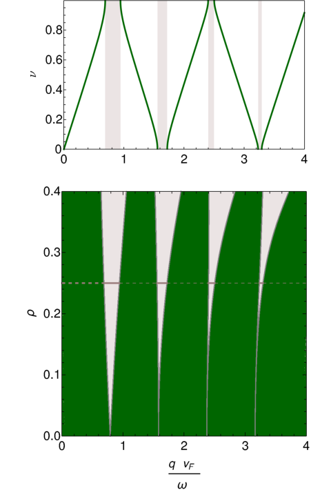
The coefficients $c_{1,2}$ are determined by the time-periodicity of steady states $|u_{n}(t)\rangle$ and operators $\beta(t)$, which also fixes the quantization condition for $\Delta$: We use Floquet’s theorem to write the solution of Eq. (10) ${f}_{-}(t)=e^{\imath\nu\tau}P_{\nu}(\tau)$ with $P_{\nu}(\tau)=P_{\nu}(\tau+\pi)$ Note3. Since $\gamma_{1/2}$ are periodic, we find that the Mathieu characteristic exponent is $\nu=2\Delta/\omega$, which must be real for stable steady states, just like for the Mathieu stability chart Kovacic et al. 2018 of Paul traps Paul 1990. From the normalization above follows $\cos(\pi\nu)={\cal C}[a,p,\pi]$, which gives (see Appendix)

and $c_{1}$ is fixed by $|\gamma_{1}|^{2}-|\gamma_{2}|^{2}=1$. Last but not least, we can use the solutions of $\gamma_{1,2}$ to uniquely define three real time periodic functions $\theta,\phi,r$, which parametrize an explicit expression of $Q(t)$ in Eq. (8) in terms of the SU(1,1) generators $J_{0}$, $J_{-}$, and $J_{+}$ in Eq. (2) Ui 1970; su11; su12

In the Appendix it is shown that $Q(t)$ in Eq. (13) gives $\tilde{H}\!=\!\Delta(b^{\dagger}_{L}b_{L}^{\phantom{\dagger}}\!\!+\!b_{R}^{\phantom{\dagger}}b_{R}^{\dagger})$ and the form of the transformed ground state $|u_{0}(t)\rangle\!\!=\!\!Q^{\dagger}|0\rangle$ is provided (see Appendix), which obeys $\beta_{L,R}(t)|u_{0}(t)\rangle=0\ \forall t$. Therefore, from Eqs. (7) and (8) all Floquet modes $|u_{n}(t)\rangle$ with $\epsilon_{n}=(n_{L}+n_{R}+1)\Delta$ are found by application of $(\beta_{L}^{\dagger}(t))^{n_{L}}(\beta_{R}^{\dagger}(t))^{n_{R}}$ on $|u_{0}(t)\rangle$.

Instability regions. Before calculating physical observables, we need to analyse the stability of the differential equations, which may not always have a solution due to the periodicity constraint. In Fig. 2(top) we plot the value of $\nu=2\Delta/\omega$ as a function of rescaled momenta $qv_{F}/\omega$ using $\bar{\rho}=-0.6$ and amplitude $\rho=0.25$. We observe that for certain regions of momenta there are no real solutions for $\Delta$. These “instability regions” will have interesting physical implications as discussed below. The stable regions are shown as a function of amplitude $\rho$ in Fig. 2(bottom) for $\bar{\rho}=-0.6$. For small $\rho$ the instability regions are equally spaced at integer values $\ell\in\mathbb{N}$ corresponding to $a=\ell^{2}$ or $\ell=2\sqrt{1+\bar{\rho}}qv_{F}/\omega$. Defining an average velocity $\bar{v}=v_{F}/\bar{K}=v_{F}\sqrt{1+\bar{\rho}}$ the instability regions therefore correspond to integer multiples of frequency which match twice the interacting dispersion relation $\ell\omega=2\bar{v}q_{\ell}$, so the physical cause can be traced to resonant excitations on the linear branches of left movers from $-\bar{v}q_{\ell}$ to right movers at $\bar{v}q_{\ell}$ and vice versa.

As shown in Fig. 3, the region of instabilities also occur for more general TLL models where the restriction $g_{2}(t)=g_{4}(t)$ in Eq. (4) is lifted Chudzinski 2016 and/or contain higher harmonics. A general analytic solution remains elusive, but the corresponding differential equation (9) is still valid, which we have solved numerically by Fourier decomposition for several parameters. Instability regions are always expected since the problem is analogous to forbidden energy regions in a band structure of a periodic potential Holthaus 2016, which is of course generic. In Fig. 3 we show the behavior of $\nu$ as a function of $qv_{F}/\omega$ for the case that only the $g_{2}$ scattering process is periodically modulated in time with $\bar{\rho}=-0.6$ and ${\rho}=0.25$ in Eq. (4) while $g_{4}=-0.4$. While quantitative changes compared to Fig. 2(top) can be identified, the regions of instabilities are again found at resonant wave vectors. In Figs. 2(top) and 3 we see that $\nu\to 1$ near the unstable regions and the ratio $c_{2}/c_{1}$ in Eq. (12) becomes singular.

To understand the physical significance of the instability regions, it is essential to consider damping. Intrinsic damping is always present in the TLL description due to higher order boson-boson interaction terms Giamarchi 2003, which lead to a finite quasiparticle life-time. A corresponding broadening of spectral peaks is seen numerically for finite energies and in finite systems Schneider et al. 2008; Bohrdt et al. 2018. The size of damping is not universal since it depends on microscopic details including the system size, but it can be assumed to be smaller than all other energy scales. In Ref. Kovacic et al. 2018 it was shown that solutions of damped Mathieu equations become always stable for amplitudes below a given threshold. We also find that a finite life-time $\tau_{0}$ in form of an imaginary energy correction $\text{Im}~\lambda_{1}=-1/\tau_{0}$ leads to convergence of instabilities as discussed below.

Results. We are now in the position to calculate physical observables. The main effect of the time periodic driving is the excitation of density waves in the steady state. The number of density excitations $b_{\chi q}^{\dagger}b_{\chi q}^{\phantom{\dagger}}$ ($\chi=L$ or $R$) in the transformed ground state $|u_{0}(t)\rangle$ is given by

In Fig. 4 we plot the time average $\bar{\eta}_{q}$. For small $q$ we find that $\bar{\eta}_{q}$ approaches the static limit, but a strong divergence is observed as the instability region around $q_{\ell}$ is approached. In the inset of Fig. 4 we exemplarily show that a finite life-time $\tau_{0}=10^{4}/v_{F}q$ turns the divergences of $\bar{\eta}_{q}$ into large maxima around $q_{\ell}$. The height of the maxima can be tuned by the product $\rho\tau_{0}$.

A universal physical picture emerges analogous to a resonance catastrophe: A finite life-time has little effect away from resonance, but the resonance response is overwhelmingly large and proportional to $\tau_{0}$. If $q_{\ell}=\ell\omega/2\bar{v}<q_{c}$ is in the TLL regime, such maxima will therefore dominate the correlations. We find that $q_{c}\sim\bar{v}m/2$ is a good estimate for the cutoff.

It is well known how TLL correlation are calculated Giamarchi 2003, which is reviewed in the Appendix for the example of density-density correlations. An overwhelming maximum of $\bar{\eta}_{q}$ will dominate the correlations and lead to long-range density order (see Appendix)

For large driving amplitudes $\rho$ the magnitude of the induced density waves can become larger than the background density, which may lead to fragementation into irregular density grains.

Discussion. The three energy scales $\omega$, $\bar{v}q_{c}$, and $v_{F}q$ determine the behavior of the system, which undergoes three different regimes as the frequency is changed:
1.) High frequencies: For $\omega\gtrsim\bar{v}q_{c}$ the instability regions are outside the TLL regime, so the physical relevant region is free of resonances. The transformation $Q$ results in a systematic change of $\bar{\eta}_{q}$ shown in Fig. 4, which approaches the static limit as $q\to 0$. The famous power-law correlations Giamarchi 2003 are corrected for intermediate distances, but the asymptotic static limit is recovered.
2.) Intermediate frequencies: As the frequency is lowered, the resonant wave-numbers $q_{\ell}=\ell\omega/2\bar{v}$ drop below the cutoff $q_{c}$ into the TLL regime. The number of density waves $\bar{\eta}_{q_{\ell}}$ becomes very large, dominating the correlations in Eq. (16). Instead of powerlaw correlations, standing density waves at wave-numbers $q_{\ell}$ become stable throughout the system.
3.) Very low frequencies: For $\omega\ll\bar{v}q_{c}$ extended regions of instability will lead to a large number of excitations and heating, destroying the correlations.

Using typical experimental parameters for a 1D ⁸⁷Rb gas from Ref. Vogler et al. 2013 of $n=6.2\times 10^{6}/$m and $mg/n=0.6$, we arrive at $\bar{K}\approx 4$ and a cutoff of $\omega_{c}=\bar{v}q_{c}\approx 2\pi\times 1.4$kHz in the middle of the trap. Driving the perpendicular confinement with a frequency of $\omega=2\pi\times 500$Hz results in a resonance at $q_{1}=\omega/2\bar{v}=444\times 10^{3}/$m. We therefore predict a standing density wave with wavelength $\lambda=2\pi/q_{1}$ in the $\mu$m range, which is observable in real space with optical methods or an electron beam Vogler et al. 2013; Vogler et al. 2014.

The confining trapping potential leads to lower local densities $n$ near edges Vogler et al. 2013; Vogler et al. 2014 and reduced velocities $v_{F}=\pi n/m$. Everywhere $n$ agrees with the local density approximation (LDA) of TLL correlations for the local trap potential Vogler et al. 2013; Vogler et al. 2014. The trapping potential is therefore turning into an advantage: Instead of changing the frequency $\omega$, different regimes can be reached using the changing density $n$. As a function of $n$ we know $\bar{v}=\sqrt{ng/m}$ Cazalilla et al. 2011; Cazalilla 2004; Ristivojevic 2014, which in turn determines the resonant wave-vectors $q_{\ell}=\ell\omega\sqrt{m/ng}/2$ and the cutoff $q_{c}=\sqrt{ngm}/2$. Therefore, we move into the high frequency regime $q_{\ell}/q_{c}\propto\omega/ng$ as the density is lowered. Note, that the density wavenumbers $q_{\ell}$ increase near edges in contrast to Fermionic Friedel density wavenumbers, which decrease with lower densities in a trap Söffing et al. 2011. In the proposed experiment, we therefore predict standing density waves at $\lambda\sim 14\mu$m in the middle of the trap, which become shorter $\lambda\propto\sqrt{n}$ and weaker near the edge. It is an interesting open problem if significant corrections would be observed when going beyond the present LDA analysis for a typical trap size of 120 $\mu$m in Ref. Vogler et al. 2013.

Interesting many-body density excitations have been experimentally observed in driven 1D and 2D systems Zhang et al. 2020; Nguyen et al. 2019. For 1D elongated bosonic ⁷Li gases $\mu$m-size density grains emerge at $2\pi\times$80Hz driving, which were identified as stable many-body effects Nguyen et al. 2019. Experimental images show grains that appear smaller and weaker near edges which resemble features predicted above, but in a random pattern Nguyen et al. 2019. All correlations disappear for very low frequencies $\omega$. A future grain size analysis as a function of $\omega$ and $n$ may clarify if there is a relation to TLL density waves in Eq. (16).

Conclusion. We have considered time-periodically driven interacting systems in the steady state, corresponding to generic TLL models in general or the Lieb-Liniger model in particular, which e.g. applies to 1D confined atoms in ultra-cold gas experiments with tunable parameters. As we have shown, this setup is one of the very rare cases where the combination of non-equilibrium steady states with many-body physics can be analyzed in great detail. In particular, we have developed a Floquet-Bogoliubov approach by constructing time-periodic creation and annihilation operators, which solve the eigenvalue equation for the steady state by acting on the entire Floquet space. We also identify regions in frequency-momentum space where damped resonant behavior leads to a large number of density excitations. The known static powerlaw correlations Giamarchi 2003 are recovered for large distances $\gg\bar{v}/\omega$, but for frequencies below the cutoff $\bar{v}q_{c}$ characteristic density waves at integer-spaced resonant wave numbers $q_{\ell}=\ell\omega/2\bar{v}$ will become dominant.

We emphasize that the proposed Floquet-Bogoliubov algebra is completely general and can be used to solve any time-periodically driven model with Bogoliubov-type interactions exactly. The explicitly known transformation $Q$ maps all steady states onto a diagonal static oscillator basis for all times, which paves the way for a complete analysis of time-dependent effects in strongly interacting systems using a combination of powerful experimental, analytic, and numerical techniques.

References

- Jotzu et al. (2014) G. Jotzu, M. Messer, R. Desbuquois, M. Lebrat, T. Uehlinger, D. Greif, and T. Esslinger, Nature 515, 237 (2014).
- Aidelsburger et al. (2015) M. Aidelsburger, M. Lohse, C. Schweizer, M. Atala, J. T. Barreiro, S. Nascimbène, N. R. Cooper, I. Bloch, and N. Goldman, Nat. Phys. 11, 162 (2015).
- Bordia et al. (2017) P. Bordia, H. Lüschen, U. Schneider, M. Knap, and I. Bloch, Nat. Phys. 13, 460 (2017).
- Baumann et al. (2010) K. Baumann, C. Guerlin, F. Brennecke, and T. Esslinger, Nature 464, 1301 (2010).
- Mottl et al. (2012) R. Mottl, F. Brennecke, K. Baumann, R. Landig, T. Donner, and T. Esslinger, Science 336, 1570 (2012).
- Landig et al. (2015) R. Landig, F. Brennecke, R. Mottl, T. Donner, and T. Esslinger, Nat. Comm. 6, 7046 (2015).
- Klinder et al. (2015) J. Klinder, H. Keßler, M. R. Bakhtiari, M. Thorwart, and A. Hemmerich, Phys. Rev. Lett. 115, 230403 (2015).
- Landig et al. (2016) R. Landig, L. Hruby, N. Dogra, M. Landini, R. Mottl, T. Donner, and T. Esslinger, Nature 532, 476 (2016).
- Deng et al. (2014) Y. Deng, J. Cheng, H. Jing, and S. Yi, Phys. Rev. Lett. 112, 143007 (2014).
- Brennecke et al. (2008) F. Brennecke, S. Ritter, T. Donner, and T. Esslinger, Science 322, 235 (2008).
- Kulkarni et al. (2013) M. Kulkarni, B. Öztop, and H. E. Türeci, Phys. Rev. Lett. 111, 220408 (2013).
- Piazza and Ritsch (2015) F. Piazza and H. Ritsch, Phys. Rev. Lett. 115, 163601 (2015).
- Else et al. (2016) D. V. Else, B. Bauer, and C. Nayak, Phys. Rev. Lett. 117, 090402 (2016).
- Kreil et al. (2019) A. J. E. Kreil, H. Y. Musiienko-Shmarova, S. Eggert, A. A. Serga, B. Hillebrands, D. A. Bozhko, A. Pomyalov, and V. S. L’vov, Phys. Rev. B 100, 020406(R) (2019).
- Lin et al. (2009) Y.-J. Lin, R. L. Compton, K. Jiménez-García, J. V. Porto, and I. B. Spielman, Nature 462, 628 (2009).
- Aidelsburger et al. (2011) M. Aidelsburger, M. Atala, S. Nascimbène, S. Trotzky, Y.-A. Chen, and I. Bloch, Phys. Rev. Lett. 107, 255301 (2011).
- Lin et al. (2011) Y.-J. Lin, R. L. Compton, K. Jiménez-García, W. D. Phillips, J. V. Porto, and I. B. Spielman, Nat. Phys. 7, 531 (2011).
- Struck et al. (2013) J. Struck, M. Weinberg, C. Ölschläger, P. Windpassinger, J. Simonet, K. Sengstock, R. Höppner, P. Hauke, A. Eckardt, M. Lewenstein, et al., Nat. Phys. 9, 738 (2013).
- Hauke et al. (2012) P. Hauke, O. Tieleman, A. Celi, C. Ölschläger, J. Simonet, J. Struck, M. Weinberg, P. Windpassinger, K. Sengstock, M. Lewenstein, et al., Phys. Rev. Lett. 109, 145301 (2012).
- Struck et al. (2012) J. Struck, C. Ölschläger, M. Weinberg, P. Hauke, J. Simonet, A. Eckardt, M. Lewenstein, K. Sengstock, and P. Windpassinger, Phys. Rev. Lett. 108, 225304 (2012).
- Thuberg et al. (2016) D. Thuberg, S. A. Reyes, and S. Eggert, Phys. Rev. B 93, 180301(R) (2016).
- Reyes et al. (2017) S. A. Reyes, D. Thuberg, D. Pérez, C. Dauer, and S. Eggert, New J. Phys. 19, 043029 (2017).
- Thuberg et al. (2017) D. Thuberg, E. Muñoz, S. Eggert, and S. A. Reyes, Phys. Rev. Lett. 119, 267701 (2017).
- Dunlap and Kenkre (1986) D. H. Dunlap and V.-M. Kenkre, Phys. Rev. B 34, 3625 (1986).
- Grossmann et al. (1991) F. Grossmann, T. Dittrich, P. Jung, and P. Hänggi, Phys. Rev. Lett. 67, 516 (1991).
- Holthaus (1992) M. Holthaus, Phys. Rev. Lett. 69, 351 (1992).
- Grifoni and Hänggi (1998) M. Grifoni and P. Hänggi, Phys. Rep. 304, 229 (1998).
- Lignier et al. (2007) H. Lignier, C. Sias, D. Ciampini, Y. Singh, A. Zenesini, O. Morsch, and E. Arimondo, Phys. Rev. Lett. 99, 220403 (2007).
- Eckardt et al. (2009) A. Eckardt, M. Holthaus, H. Lignier, A. Zenesini, D. Ciampini, O. Morsch, and E. Arimondo, Phys. Rev. A 79, 013611 (2009).
- Rapp et al. (2012) A. Rapp, X. Deng, and L. Santos, Phys. Rev. Lett. 109, 203005 (2012).
- Wang et al. (2020) T. Wang, S. Hu, S. Eggert, M. Fleischhauer, A. Pelster, and X.-F. Zhang, Phys. Rev. Res. 2, 013275 (2020).
- Bretin et al. (2004) V. Bretin, S. Stock, Y. Seurin, and J. Dalibard, Phys. Rev. Lett. 92, 050403 (2004).
- Schweikhard et al. (2004) V. Schweikhard, I. Coddington, P. Engels, S. Tung, and E. A. Cornell, Phys. Rev. Lett. 93, 210403 (2004).
- Ramos et al. (2008) E. R. F. Ramos, E. A. L. Henn, J. A. Seman, M. A. Caracanhas, K. M. F. Magalhães, K. Helmerson, V. I. Yukalov, and V. S. Bagnato, Phys. Rev. A 78, 063412 (2008).
- Pollack et al. (2010a) S. E. Pollack, D. Dries, R. G. Hulet, K. M. F. Magalhães, E. A. L. Henn, E. R. F. Ramos, M. A. Caracanhas, and V. S. Bagnato, Phys. Rev. A 81, 053627 (2010a).
- Wang et al. (2014) T. Wang, X.-F. Zhang, F. E. A. d. Santos, S. Eggert, and A. Pelster, Phys. Rev. A 90, 013633 (2014).
- Greschner et al. (2014) S. Greschner, L. Santos, and D. Poletti, Phys. Rev. Lett. 113, 183002 (2014).
- Meinert et al. (2016) F. Meinert, M. J. Mark, K. Lauber, A.J. Daley, and H.-C. Nägerl, Phys. Rev. Lett. 116, 205301 (2016).
- Arimondo et al. (2012) E. Arimondo, D. Ciampini, A. Eckardt, M. Holthaus, and O. Morsch, in vol. 61 p. 515 of Advances in Atomic, Molecular, and Optical Physics, edited by P. Berman, E. Arimondo, and C. Lin (Academic Press, 2012).
- Keilmann et al. (2011) T. Keilmann, S. Lanzmich, I. McCulloch, and M. Roncaglia, Nat. Comm. 2, 361 (2011).
- Greschner and Santos (2015) S. Greschner and L. Santos, Phys. Rev. Lett. 115, 053002 (2015).
- Tang et al. (2015) G. Tang, S. Eggert, and A. Pelster, New J. Phys. 17, 123016 (2015).
- Sträter et al. (2016) C. Sträter, S. C. L. Srivastava, and A. Eckardt, Phys. Rev. Lett. 117, 205303 (2016).
- Lange et al. (2017) F. Lange, S. Ejima, and H. Fehske, Phys. Rev. Lett. 118, 120401 (2017).
- Eckardt et al. (2005) A. Eckardt, C. Weiss, and M. Holthaus, Phys. Rev. Lett. 95, 260404 (2005).
- Eckardt and Anisimovas (2015) A. Eckardt and E. Anisimovas, New J. Phys. 17, 093039 (2015).
- Eckardt (2017) A. Eckardt, Rev. Mod. Phys. 89, 011004 (2017).
- Giamarchi (2003) T. Giamarchi, Quantum Physics in One Dimension (Clarendon Press - Oxford, 2003).
- Kinoshita et al. (2004) T. Kinoshita, T. Wenger, and D. S. Weiss, Science 305, 1125 (2004).
- Paredes et al. (2004) B. Paredes, A. Widera, V. Murg, O. Mand el, S. Fölling, I. Cirac, G. V. Shlyapnikov, T. W. Hänsch, and I. Bloch, Nature (London) 429, 277 (2004).
- Vogler et al. (2013) A. Vogler, R. Labouvie, F. Stubenrauch, G. Barontini, V. Guarrera, and H. Ott, Phys. Rev. A 88, 031603(R) (2013).
- Vogler et al. (2014) A. Vogler, R. Labouvie, G. Barontini, S. Eggert, V. Guarrera, and H. Ott, Phys. Rev. Lett. 113, 215301 (2014).
- Pollmann et al. (2013) F. Pollmann, M. Haque, and B. Dóra, Phys. Rev. B 87, 041109(R) (2013).
- Bernier et al. (2014) J.-S. Bernier, R. Citro, C. Kollath, and E. Orignac, Phys. Rev. Lett. 112, 065301 (2014).
- Chudzinski and Schuricht (2016) P. Chudzinski and D. Schuricht, Phys. Rev. B 94, 075129 (2016).
- Pielawa (2011) S. Pielawa, Phys. Rev. A 83, 013628 (2011).
- Graf et al. (2010) C. D. Graf, G. Weick, and E. Mariani, EPL (Europhysics Letters) 89, 40005 (2010).
- Bukov and Heyl (2012) M. Bukov and M. Heyl, Phys. Rev. B 86, 054304 (2012).
- Kagan and Manakova (2009) Y. Kagan and L. A. Manakova, Phys. Rev. A 80, 023625 (2009).
- Chudzinski (2016) P. Chudzinski, arXiv:1607.00995 (2016).
- Lieb and Liniger (1963) E. H. Lieb and W. Liniger, Phys. Rev. 130, 1605 (1963).
- Olshanii (1998) M. Olshanii, Phys. Rev. Lett. 81, 938 (1998).
- Cazalilla et al. (2011) M. A. Cazalilla, R. Citro, T. Giamarchi, E. Orignac, and M. Rigol, Rev. Mod. Phys. 83, 1405 (2011).
- Cazalilla (2004) M. A. Cazalilla, J. Phys. B: At. Mol. Opt. Phys. 37, S1 (2004).
- Ristivojevic (2014) Z. Ristivojevic, Phys. Rev. Lett. 113, 015301 (2014).
- Ui (1970) H. Ui, Progress of Theoretical Physics 44, 703 (1970).
- (67) D.R. Truax, Phys. Rev. D31, 1988 (1985).
- (68) J. Garcia and R. Rossignoli, Phys. Rev. A96, 062130 (2017).
- Sólyom (1979) J. Sólyom, Adv. Phys. 28, 201 (1979).
- (70) The applied fields are not necessarily purely sinosoidal, but or can be obtained exactly for a given situation and therefore also the required fields. For small amplitudes a linear expansion will generally also result in sinosoidal fields.
- Holthaus (2016) M. Holthaus, J. Phys. B: At. Mol. Opt. Phys. 49, 013001 (2016).
- Notes (a) While the Floquet problem always becomes static in the extended Floquet Hilbert space using frequency decomposition Eckardt and Anisimovas 2015, we seek to obtain a static diagonal solution in the original Hilbert space and a transformation for all times.
- (73) Here, is also analogous to the quasimomentum in the well-known bandstructure of a cosine-potential Holthaus 2016.
- Kovacic et al. (2018) I. Kovacic, R. Rand, and S. M. Sah, Appl. Mech. Rev. 70, 020802 (2018).
- Paul (1990) W. Paul, Rev. Mod. Phys. 62, 531 (1990).
- Schneider et al. (2008) I. Schneider, A. Struck, M. Bortz, and S. Eggert, Phys. Rev. Lett. 101, 206401 (2008).
- Bohrdt et al. (2018) A. Bohrdt, K. Jägering, S. Eggert, and I. Schneider, Phys. Rev. B 98, 020402(R) (2018).
- Söffing et al. (2011) S. A. Söffing, M. Bortz, and S. Eggert, Phys. Rev. A 84, 021602(R) (2011).
- Nguyen et al. (2019) J. H. V. Nguyen, M. C. Tsatsos, D. Luo, A. U. J. Lode, G. D. Telles, V. S. Bagnato, and R. G. Hulet, Phys. Rev. X 9, 011052 (2019).
- Zhang et al. (2020) Z. Zhang, K. Yao, L. Feng, J. Hu, and C. Chin, Nat. Phys. 16, 652 (2020).