$f(T)$ cosmology: From Pseudo-Bang to Pseudo-Rip

Let us first investigate the conditions for the standard non-singular bounce realization. As it is known, this can be generated by employing a scale factor of the form Novello:2008ra

where the constant $a_{B}\equiv a(t_{B})$ is the minimal scale factor at the bounce point $t_{B}$ and $\alpha$ is a positive parameter with dimensions [T]^-2. Moreover, $\gamma$ is the barotropic index related to the equation-of-state parameter of the cosmic fluid as

where $p$ and $\rho$ are the pressure and energy density respectively. Hence, for positive $\gamma,\alpha$ the above scale factor is indeed non-singular for finite times. As one can see, the scale factor (1) generates a symmetric phase portrait about $H=0$ axis ElHanafy:2017sih; Awad:2017yod

where $\dot{H}_{+}$ ($\dot{H}_{-}$) denotes the branch $\dot{H}>0$ ($\dot{H}<0$).

The non-singular bouncing cosmology phase portrait (3) is characterized by a double valued function, as presented in Fig. 21(a). Since the universe cannot reach the Minkowskian origin at a finite time, the universe is non-singular. We mention that the bounce occurs at $H=0$ where $\dot{H}$ is positive. In fact, the $\dot{H}>0$ regions require an effectively phantom cosmology. However, the crossing between phantom and non-phantom phase is possible only wherever the phase portrait is double-valued and has vertical slope at the crossing points (fixed points)¹¹ 1 The conditions to reach a fixed point in a finite time has been discussed in Awad:2013tha (also see Awad:2017yod).. Furthermore, it is obvious that the universe cannot result to a late-time accelerated expansion phase. This can be clearly seen in Fig. 21(a), since the last phase of the portrait on the $\dot{H}_{-}$ branch remains in the shaded region III eternally Awad:2017yod; ElHanafy:2017xsm.

Let us try to modify the scale factor (1) to additionally obtain late-time accelerated expansion. One could think to impose a positive cosmological constant $\Lambda$ similarly to $\Lambda$CDM cosmology. This would impose a vertical shift of the phase portrait of Fig. 21(a) slightly upwards. Thus, the universe begins at a de Sitter phase with negative $H=-H_{de}$, evolving towards another de Sitter phase with positive $H=+H_{de}$ instead of the Minkowski phase at $H=0$. However, the new feature is that the fixed points at the left and right boundaries of the portrait, i.e. at $H=\pm H_{max}$ where $H_{max}$ is the maximum value of the Hubble parameter, will not have infinite slopes anymore, and therefore the transition between phantom and non-phantom regimes, namely between $\dot{H}_{+}$ and $\dot{H}_{-}$ branches, cannot occur in a finite time. Thus, we need to find an alternative way to unify bounce and late-time acceleration. This is done in the following.

Since adding by hand a positive constant is not efficient, we proceed modifying the standard bounce scale factor (1) by introducing a correction exponential function as

where $a_{k}$ and $t_{i}$ are constants and $\beta$ is a positive dimension-full parameter with dimensions [T]^-1, whereas the modified scale factor (4) reduces to the usual bouncing model by setting $\beta=0$. Unlike the bounce scale factor which has one local minimum at bounce $t=t_{B}$, the modified scale factor has a local minimum and local maximum at $t=t_{i}-\frac{1}{3\beta\gamma}\pm\frac{\sqrt{\alpha(\alpha-6\beta^{2}\gamma)}}{\alpha\beta\gamma}$, which implies that $\alpha>6\beta^{2}\gamma$. In fact, these local critical points are associated with turnaround and bounce phases. The Hubble parameter corresponding to (4) is

and its first derivative reads

Note that these expressions remain finite for positive $\gamma,\alpha$, i.e in the case where the bounce is non-singular. Inverting the above expression we acquire

and thus inserting into (6) we obtain the phase portrait equation

Note that $H=\beta$ is a fixed point and the time required to reach it is infinite.

The phase portrait graph of (8) is given in Fig. 21(b), which indeed shows that $H$ and $\dot{H}$ values are always finite. Moreover, we obtain fixed points, namely having $\dot{H}=0$, at $H=\beta$ (de Sitter origin) and at maximum positive and minimum negative values of the Hubble parameter $H=\pm\sqrt{\frac{\alpha}{6\gamma}}+\beta$, respectively. We note that in a viable scenario, one needs $|H|_{\textrm{max}}\gg\beta$ and subsequently $\alpha\gg 6\beta^{2}\gamma$. As it is clear from the graph, the modified scale factor (4) shifts the phase portrait symmetry from line $H=0$ to $H=\beta$. As a result, the Minkowskian origin of the conventional bounce is shifted to a de Sitter one, however this has crucial consequences on the cosmic evolution as we will discuss in Sec. 3. We mention that in this schematic graphical representation we have exaggerated the value of the parameter $\beta$ in Fig. 21(b), in order to show clearly the breaking of the symmetry around $H=0$. However, as we will see later on, when confronting with observational data the value of $\beta$ will be a small positive number, and the deformation seen in 21(b) will be small, but still effective.

In the final phase of the portrait of Fig. 21(b), the universe evolves towards a de Sitter fixed point at $H=\beta$, providing a late accelerated expansion phase. In addition, the fixed points at the phase portrait boundaries, $H=\pm H_{max}$, are still having infinite slopes which is a necessary condition to allow for the crossing of the phantom divide in a smooth way (a detailed analysis of the phase portrait is given in Section 3).

In summary, up to now we have achieved our target to unify bounce and late acceleration in a single scenario. The last step is to determine the model parameters in order to obtain a viable scenario. The above scenario contains the four parameters $a_{k}$, $t_{i}$, $\alpha$ and $\beta$, in addition to the barotropic index (equation of state) parameter $\gamma$, which takes the values $\gamma=1$ for dust matter and $\gamma=4/3$ for radiation. In order determine their values, one should thus choose four conditions from the observed universe history.

In standard Big Bang cosmology there is the initial singularity at cosmic time $t=0$. However, since in our case $-\infty<t<\infty$ it proves convenient to set $t=0$ at the fixed point $\dot{H}=0$ with $H_{max}=\sqrt{\frac{\alpha}{6\gamma}}+\beta$, which is identified with point $G$ on the phase portrait of Fig. 21(b). From now on all time identifications are calculated from the fixed point $G$. This choice enables us to confront the model with the standard observational requirements of the cosmic thermal history. Imposing the fixed point phase condition $\dot{H}=0$ in Eq. (6) and solving for the cosmic time $t$ we acquire

where $t^{-}$ ($t^{+}$) identifies the fixed point phase at $H<0$ ($H>0$) regime at point $E$ ($G$) of the phase portrait Fig. 21(b). Setting $t^{+}=0$ as illustrated above, we determine that

Therefore, we find that $t^{-}=2t_{i}=-2\sqrt{\frac{2}{3\gamma\alpha}}$ at point $G$. This is the first out of the four conditions. For the other three we choose:
(i) For the present time we choose $t_{0}\approx 4.3\times 10^{17}$ s as it arises from standard cosmology, and we moreover normalize the present scale factor to $a_{0}=a(t_{0})=1$.
(ii) At the end of inflation (point $K$ on Fig. 21(b)), which corresponds to zero acceleration $\ddot{a}=0$ we need to have $t\sim 10^{-32}$ s as expected from standard cosmology.
(iii) For the late-time transition from deceleration to acceleration (point $L$), where the acceleration is again zero, namely $\ddot{a}=0$, we impose a time $t\sim 2.4\times 10^{17}$ s, which is consistent with the observed transition redshift $z_{tr}\sim 0.6-0.8$ Capozziello:2015rda. Finally, alongside conditions (i) and (iii) we consider $\gamma=1$ as cold dark matter is expected to dominate the evolution, while for condition (ii) we impose $\gamma=4/3$ as radiation is expected to be dominant at the reheating phase by the end of inflation. Hence, we conclude that

while inserting into (10) we find

The numerical results show that $\alpha\gg 6\beta^{2}\gamma$, confirming the viability condition in order to have $|H|_{\textrm{max}}\gg\beta$, and also verifying that the modified scale factor (4) should have not only a local minimum as in the bounce scenario but also a local maximum which is associated with a turnaround phase. In the following we revisit these phases among other interesting features in more detail by investigating the corresponding phase portrait.

According to the phase portrait the cosmic time flows clockwise, where the origin has been shifted from Minkowski to a semi-stable de Sitter fixed point $A$, at which $H=\beta\sim 4.1\times 10^{-43}$ GeV and $\dot{H}=0$. Using the phase portrait equation (8), the flow time from any phase point $H_{0}\lesssim\beta$ on the $\dot{H}_{-}$ branch can be calculated by

since $1\leq\gamma\leq 2$ to maintain the stability and the causality conditions. Therefore, the universe is eternal and has no initial finite-time singularity. It is straightforward to show that the time asymptotic of the scale factor (4) and the Hubble parameter (5) are respectively

given that $\beta>0$ and $\alpha>0$.

We mention that in the standard bounce the scale factor diverges as $t\to-\infty$. On the other hand, in standard Big Bang cosmology the initial scale factor $a(t)\to 0$ and $H(t)\to\infty$ as $t\to 0$. On the contrary, in the pure cosmological constant universe, the Hubble parameter has a finite constant value, but the universe cannot exhibit a decelerated expansion phase. Hence, one can realize that the present scenario is a novel one, in which the universe initial state is intermediate between the Big Bang and the de Sitter universe. Inspired by the Pseudo-Rip terminology (see below) we call this eternal phase as Pseudo-Bang, since it is characterized by $a(t)\to 0$ and $H(t)\to const.>0$ as $t\to-\infty$ (note that this is different from the emergent universe scenario which is characterized by $a(t)\to const.$ at $t\to-\infty$ Ellis:2002we; Mulryne:2005ef). This is the first phase of the scenario at hand.

Following the phase portrait of Fig. 21(b) clockwise, we identify the interval (i), which ends at point $B$, in which the portrait cuts the zero acceleration curve $\dot{H}_{-}=-H^{2}$. Since the Hubble values are positive (as given in Table 1, $2.4\times 10^{-43}\lesssim H(t)\lesssim 4.1\times 10^{-43}$ GeV) in this interval, and $\dot{H}_{-}>-H^{2}$, the universe expands with acceleration. Such an unconventional initial phase represents a non-singular inflationary phase, unlike standard bounce cosmology which begins with a decelerated contraction phase. This is the second phase of the scenario at hand.

Remarkably this quasi de Sitter inflationary phase runs at low energy level which in effect might contribute to solve the theoretical problem of the cosmological constant. Additionally, since this phase is eternal, it has enough time to solve the usual problems of the Standard Model of cosmology. Furthermore, there is no need to compute the minimum $e$-fold number, $N=-\ln(a_{i}/a_{f})$, since $a_{i}$ can always be chosen small enough to obtain a suitable $N$. On the other hand, in the scenario at hand the comoving Hubble radius $R_{H}=\frac{1}{a(t)|H(t)|}$, which we refer to as horizon, is infinite at the Pseudo-Bang origin as $a(t)\to 0$. Therefore, all modes are at sub-horizon scale $k\gg R_{H}^{-1}$, or equivalently the physical wavelengths $\lambda\ll\lambda_{H}$, where $\lambda(t)=a(t)/k$ is the physical mode wavelength $\lambda_{H}=|H^{-1}|$ is the Hubble radius (we refer to the Hubble radius at Pseudo-Bang as $\lambda_{\beta}\to 1/\beta$). This is a necessary condition to have an initial causal universe. Consequently, we can assume that the primordial fluctuations are coherent, as indicated by the observations of acoustic peaks in the power spectrum of Cosmic Microwave Background (CMB) anisotropies. In this case, it is natural to assume that the quantum fluctuations around the initial vacuum state form the Bunch-Davies vacuum Bunch:1978yq. The evolution of the physical modes at different scales verses Hubble horizon is given in Fig. 3.

At point $C$ on Fig. 21(b) the universe goes from dynamical region III (decelerated expansion) to another dynamical region II (decelerated contraction). Therefore, point $C$ represents a turnaround point, $H=0$ and $\dot{H}_{-}<0$, at which the universe reaches a maximum size with a finite deceleration unlike Big Brake models Keresztes:2012zn. This is the third phase of the scenario at hand.

At the turnaround point $C$, the Hubble parameter goes to zero. Using (5), (11) and (12), we determine the time at the turnaround as

Notably, in general relativity, at turnaround phase one should introduce unconventional matter species violating the null energy condition. This situation can be avoided in modified gravity making the gravitational sector to compensate the matter component at the turnaround point Cai:2011bs. Finally, we mention that Fig. 3 shows that the corresponding Hubble radius $\lambda_{H}$ becomes infinite, allowing the modes to re-enter the horizon and become sub-horizon again.

At point $D$, the phase portrait intersects the zero acceleration curve $\dot{H}_{-}=-H^{2}$ for the second time, but at a negative value of $H\sim-6.4\times 10^{6}$ GeV, as given in Table 1. The, the universe enters in a new phase of accelerated contraction $\dot{H}_{-}>-H^{2}$, namely interval (iv). Notably, the point $E$ is a fixed point which exceptionally can be reached in finite time. This can be proven, since

Additionally the phase portrait is double valued about $E$ which is a necessary condition to cross the phantom divide line through point $E$, for more detail see Awad:2013tha; Awad:2017yod. At this point $E$, we calculate $H_{E}=\beta-\frac{\sqrt{\alpha}}{3\gamma}\sim-6.8\times 10^{6}$ GeV, then the time to reach is $t_{E}=2t_{i}=-2\sqrt{\frac{2}{3\gamma\alpha}}\sim-4.8\times 10^{-32}$ s. This Phantom crossing I phase is the fourth epoch of the scenario at hand.

At point $F$ the universe bounces from an accelerated contraction to accelerated expansion in an effective phantom regime, where $\dot{H}_{+}>0$, as it is shown in Fig. 21(b). Using (5) and (10), we determine the time at the bounce point as

At the bounce point $F$ one should investigate two major problems that are usually facing such models in GR: The first is known as ghost instability due to violation of the null energy condition, which has been shown to be avoided within modified gravity framework whereas the matter sector remains casual and stable Cai:2011tc; Bamba:2016gbu. The second is more severe and called the anisotropy problem since any small anisotropy evolves as $\propto a(t)^{-6}$ and becomes dominant during the contraction phase at suitably small scale factors, thus destroying FLRW geometry Novello:2008ra. Nevertheless, the usual way for its avoidance is the introduction of a super-stiff matter component $\gamma\gg 2$ which scales as $a(t)^{-3\gamma}$ and thus it grows faster and dominates over the anisotropy. This being the case as we will discuss this later on in Subsection 4.2. This bouncing phase is the fifth phase in the scenario at hand.

Similar to the phase at the fixed point $E$, it can be shown that

Then, the fixed point $G$ can be reached in a finite time, whereas the portrait is double valued about it. Therefore, at the phase point $G$, the universe crosses the phantom divide line for the second time, similarly to point $E$, but this time from phantom to non-phantom phase. At that point the Hubble parameter $H_{G}=\beta+\frac{\sqrt{\alpha}}{3\gamma}\sim 6.8\times 10^{6}$ GeV. We stress that we have set the time at point $G$ as $t_{G}=0$ as discussed in detail in Subsection 2.2. The Phantom crossing II is the sixth phase of the evolution.

During the interval (vii) the universe evolves into quintessence regime just as in standard inflationary models. In the latter, the universe needs to enlarge itself around $10^{28}$ times ($\sim 60$ $e$-folds) to solve the horizon and flatness problems of standard cosmology Olive:1989nu. However, in our scenario there is no need for this restriction, since the preceding phases are sufficient to solve these problems. Indeed, the model predicts just few $e$-folds during this accelerated expansion period as indicated in Table 1. Additionally, as the Table shows, the energy scales are $H\sim 10^{6}$ GeV and $E\sim 10^{12}$ GeV at the graceful exit point, that is below the energy scale of the grand unified theory (GUT), and hence monopoles are not going to be produced, thus bypassing the monopole problem of standard cosmology. Moreover, as it has been shown, the scale invariant power spectrum can be produced in standard bouncing cosmology in the contraction phase, which occurs in the scenario at hand too. At the end of this interval, at point $K$, the universe gracefully exits into a decelerated expansion phase, which characterizes standard cosmology. This smooth transition period is essential to prepare the universe to begin the hot Big Bang nucleosynthesis process. The graceful exit from inflation II is the seventh phase of the present scenario.

The eighth phase of the universe evolution is the standard cosmology phase of reheating, radiation and matter epochs. In this case, it is convenient to examine the behaviour of the phase portrait (8) at relevant epochs. In particular, for the $\dot{H}_{-}$ branch at $H\gg\beta$, we obtain the leading term $\dot{H}_{-}=-\frac{3}{2}\gamma H^{2}$ which reproduces the power-law standard cosmology phase portrait.

In order to obtain a fuller view and to examine the capability of the present scenario to predict a successful thermal evolution, we define the entropy $S$ of all particles in thermal equilibrium at temperature $\Theta$ in volume $V$. According to the first law of thermodynamics, in the expanding universe we have

with the integrability condition $\frac{\partial^{2}S}{\partial\Theta\partial V}=\frac{\partial^{2}S}{\partial V\partial\Theta}$ Weinberg:1972kfs, where the energy density and pressure satisfy

From the matter conservation equation $\dot{\rho}+3\gamma H\rho=0$ it is implied that $\rho\propto a^{-3\gamma}$. Solving (18) we evaluate the temperature as $\Theta(t)=\Theta_{0}~a(t)^{-3(\gamma-1)}$, with $\Theta_{0}\equiv\Theta(t_{0})$ an arbitrary constant. Hence, this finally leads to

We choose a boundary condition such that the temperature $\Theta\sim 2.73$ K at the present time $t_{0}\sim 10^{17}~\textmd{s}>t_{eq}$, with a dust equation-of-state parameter $\gamma=1$. This determines the value $\Theta_{0}=2.73$ K.

In summary, at the contracting Pseudo-Bang phase the temperature increases and peaks up at the bounce point with $\Theta\sim 10^{27}$ K (assuming relativistic species with barotropic index $\gamma\approx 1.28$), and then it decreases following the standard thermal history. In Fig. 4 we depict the temperature evolution of the Pseudo-Bang scenario on top of the corresponding one for the standard Big-Bang cosmology (we restrict the graph to the interval from Planck era to the radiation-matter equality, which is suitable for comparison since at later times both scenarios exhibit the same behaviour, namely the same matter epoch.

The ninth phase of the scenario at hand is the late-time acceleration. In particular, on the phase portrait of Fig. 21(b) one can see that the universe exhibits a late-time transition from deceleration to acceleration, as indicated by point $L$. At this point, the phase portrait crosses the zero acceleration curve for the last time, from $\dot{H}_{+}<-H^{2}$ decelerated expansion region into $\dot{H}_{+}>-H^{2}$ accelerated expansion, where $H>0$ and $\dot{H}_{+}<0$. More precisely, we determine the current value of the Hubble parameter as expected, by taking the present time $t_{0}=4.3\times 10^{17}$ s (which is consistent with the assumption $a(t_{0})=1$ or equivalently of redshift $z(t_{0})=\frac{1}{a(t_{0})}-1=0$) and according to the estimated values of the model parameters (11), (12), and thus the Hubble function (5) gives the present Hubble value $H_{0}\approx 66.6$ km/s/Mpc. Moreover, it is straightforward to show that at the deceleration-to-acceleration transition time $t_{L}=2.4\times 10^{17}$ s the corresponding redshift $z_{tr}=\frac{1}{a(t_{L})}-1\approx 0.7$ lies within 1$\gamma$ agreement with its measured value $z_{tr}=0.72\pm 0.05$ for $H_{0}=68\pm 2.8$ km/s/Mpc Farooq:2016zwm. The late acceleration is labeled on the phase portrait as interval (ix), and is confined between points $L$ and $A$. Notably, this last phase cannot be exhibited in the standard bounce of Fig. 21(a), where the universe continues the decelerated expansion eternally.

As we observe in Fig. 21(b), the phase portrait evolves towards the fixed point $A$ as a final fate. Similarly to (13), the time needed to reach that point in infinite. Given that $\beta>0$ and $\alpha>0$, the time asymptotic of the scale factor (4) and Hubble (5) have the limits $a(t)\to\infty$ and $H(t)\to\beta^{+}$ as $t\to\infty$. Among four possible final phases of expanding universe classified in Ref. Frampton:2011aa, we deduce that in the scenario at hand the universe evolves towards a Pseudo-Rip which is an intermediate between the no Rip and the Little Rip. This phase is characterized by a monotonically increasing Hubble to a constant value, producing an inertial force which does not increase monotonically but peaks up at a particular future time and then decreases. In this case the bound structures dissociate if they are at or below a particular threshold that depends on the inertial force, for more details see Subsection 4.2. This is the tenth and final phase.

Recalling the Pseudo-Bang scale factor (4), one may realize that the hypersurface at the Pseudo-Bang $t=-\infty$ is not space-like but null. In this sense, the Pseudo-Bang resembles the de Sitter universe up to a sub-leading term, as it is clear from (5). Similarly to de Sitter, there can be particles coming to Pseudo-Bang from the other part of spacetime. To reveal the similarity between the Pseudo-Bang phase and de Sitter universe, we impose the transformation

where $\tau\to\pm\infty$ as $\tilde{t}\equiv t-t_{i}\to\pm\infty$, which leads to the Pseudo-Bang scale factor as $a(\tau)=e^{\beta\tau}$. Moreover, we write

which implies that $d\tau$ differs from $d\tilde{t}$ by a sub-leading term only, and thus $d\tau/d\tilde{t}\to 1$ as $\tilde{t}\to\pm\infty$ ($\tau\to\pm\infty$). In this case, we write the FLRW metric at Pseudo-Bang/Rip as

The symmetry of the obtained spacetime can be revealed by making use of a flat embedding of (22) into a 5-dimensional Minkowski spacetime,

which can be realized as the hyperboloid

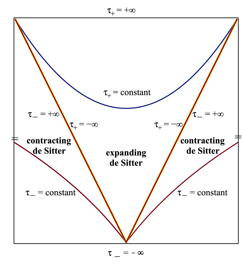
For the coordinate transformation²² 2 We use $-\infty<\tau_{+}<\infty$ to identify the expanding patch which represents only one-half of the entire de Sitter space, while $-\infty<\tau_{-}<\infty$ will be used to describe the other contracting patch.

the induced metric is

This shows that the above metric covers only half of the de Sitter spacetime, where Eqs. (25) restrict the spacetime configuration to the region $X_{0}+X_{4}=\beta^{-1}e^{\beta\tau_{+}}\geq 0$, that is the expanding Poincaré patch (EPP). The other half, $X_{0}+X_{4}\leq 0$, is covered by the metric

which represents the contracting Poincaré patch (CPP).

The entire manifold at Pseudo-Bang and Pseudo-Rip can be obtained via a Penrose–Carter diagram, as seen in Fig. 54(a). This diagram reveals that the boundary between the EPP and the CPP at $\tau_{\pm}=\mp\infty$ is light-like. Note that the solution is invariant under the transformations $t_{+}\to-t_{-}$ and $\beta\to-\beta$. In terms of the phase-portrait terminology, one obtains that the phase portrait equation (8) may have another fixed point of de Sitter type at $H=-\beta$. In Subsection 3.1, we discussed the evolution corresponding to the expanding de Sitter origin, i.e. $H=+\beta$, as realized by the phase portrait of Fig. 21(b). Since the Pseudo-Bang resembles the de Sitter case, and $t\to-\infty$ is a null hypersurface, it may not represent a genuine beginning. For that reason we label the time of the portrait with the origin at $H=\beta$ as $-\infty<t_{+}<\infty$. On the other hand, we label the time of the portrait with origin at $H=-\beta$ as $-\infty<t_{-}<\infty$, as seen in Fig. 54(b). One realizes that there is no need for junction conditions to match the two phases at $H=\pm\beta$. Indeed, the Pseudo-Bang in the expanding de Sitter (i.e. EPP), $t_{+}\to-\infty$, $a(t_{+})\to 0$ and $H(t_{+})\to\beta^{-}$, is naturally matched with the contracting de Sitter (i.e. CPP), $t_{-}\to+\infty$, $a(t_{-})\to 0$ and $H(t_{-})\to-\beta^{+}$. On the other hand, the Pseudo-Rip in the expanding de Sitter (i.e. EPP), $t_{+}\to+\infty$, $a(t_{+})\to\infty$ and $H(t_{+})\to\beta^{+}$, is naturally matched with the contracting de Sitter (i.e. CPP), $t_{-}\to-\infty$, $a(t_{-})\to\infty$ and $H(t_{-})\to-\beta^{-}$.

For the moment the whole analysis remains at the kinematic level, namely at the investigation of the required Hubble function evolution. Nevertheless, one should consider the phase portrait (8) as a field equation governing the dynamics of FLRW cosmology. Therefore, one should provide the theory, namely a modified gravity, that could dynamically produce such a Pseudo-Bang scenario. Amongst the different classes of gravitational modification there is one, i.e. $f(T)$ gravity, which has second-order fields equations and thus it allows for the construction of the phase portrait in a simple way Awad:2017yod (in the particular case of Pseudo-Bang scenario the phase portrait should be (8)). Hence, in the following section we investigate the realization of the Pseudo-Bang scenario in the framework of $f(T)$ gravity. Notably, the junction conditions in $f(T)$ gravity has been investigated in (delaCruz-Dombriz:2014zaa), and used to match two branches of a phase portrait, see (Awad:2017sau). However, in our case, the matching between the EPP and CPP is naturally fulfilled with no need of junction conditions.

In the torsional formulation of gravity it proves convenient to use as dynamical variables the vierbeins fields ${\mathbf{e}_{A}(x^{\mu})}$, which at each manifold point $x^{\mu}$ form an orthonormal basis. In a coordinate basis they can be expressed as $\mathbf{e}_{A}=e^{\mu}_{A}\partial_{\mu}$, related to the metric through

with Greek and Latin indices respectively running over coordinate and tangent space. One introduces the Weitzenböck connection $\overset{\mathbf{w}}{\Gamma}{{}^{\lambda}}_{\nu\mu}\equiv e^{\lambda}_{A}\>\partial_{\mu}e^{A}_{\nu}$ Weitzenb23, and therefore the resulting torsion tensor reads

This torsion tensor contains all the geometrical information, and thus it describes the gravitational field. Through its contraction one acquires the torsion scalar

which is then used as the Lagrangian of the theory. Variation of the action in terms of the vierbeins gives identical equations with general relativity, and that is why this theory was named teleparallel equivalent of general relativity Pereira.book.

Inspired by the curvature modifications of gravity, in which one generalizes the Einstein-Hilbert action, one can start from teleparallel equivalent of general relativity and extend the Lagrangian to an arbitrary function of the torsion scalar $T$. The resulting $f(T)$ gravity is characterized by the action Cai:2015emx

with $e=\text{det}(e_{\mu}^{A})=\sqrt{-g}$, $\kappa^{2}=8\pi G$ the gravitational constant, and where for completeness we have added the matter Lagrangian $L_{m}$. Variation of the action (31) with respect to the vierbein gives Cai:2015emx

with $f_{T}:=\frac{df}{dT}$ and $f_{TT}:=\frac{d^{2}f}{dT^{2}}$. Additionally, we have defined the superpotential

which is skew symmetric in the last pair of indices, as well as the energy-momentum tensor of the total matter fields (baryonic and dark matter and radiation) ${\mathfrak{T}_{\mu}}^{\nu}=e{{}^{a}}{{}_{\mu}}\left(-\frac{1}{e}\frac{\delta\mathcal{L}_{m}}{\delta e{{}^{a}}{{}_{\nu}}}\right)$, assumed it to be of a perfect fluid form

with $u_{\mu}=\delta_{\mu}^{t}$ the fluid 4-velocity, and $\rho$ and $p$ the energy density and pressure in its rest frame.

In order to apply $f(T)$ gravity to a cosmological framework we consider the flat Friedmann-Lemaître-Robertson-Walker (FLRW) geometry

which corresponds to the vierbein choice $e_{\mu}^{A}={\text{d}iag}(1,a,a,a)$, with $a(t)$ the scale factor (we impose the natural units $c=\hbar=k_{B}=1$, while $\kappa=1/M_{p}$ with $M_{p}=2.4\times 10^{18}$ GeV the reduced Planck mass). Inserting into (32) we extract the Friedmann equations as

where we have also made use of the useful relation that provides the torsion scalar in FLRW geometry, namely

Additionally, assuming a barotropic equation of state for the matter fields of the form (2), namely $p=(\gamma-1)\rho$, the matter conservation equation reads

Note that the above Friedmann equations for $f(T)=T-2\Lambda$ (with $\Lambda>0$) coincide with $\Lambda$CDM cosmology.

As it was discussed in the Introduction, one of the advantages of $f(T)$ gravity is that the Friedmann equation (36) gives $\rho\equiv\rho(H)$. Consequently, the differential equation (37) represents a one-dimensional autonomous system of the form $\dot{H}\equiv\mathcal{F}(H)$ as long as the equation of state $p\equiv p(\rho)$ is assumed. Hence, we can always interpret it as a vector field on a line, applying one of the basic techniques of dynamics by drawing $\dot{H}$ versus $H$, which helps to analyze the cosmic model in a clear and transparent way even without solving the system. In order to fix our notation we follow book:Steven calling the above equation the phase portrait, while its solution $H(t)$ is the phase trajectory. Thus, the phase portrait corresponds to any theory which can be drawn in an ($\dot{H}-{H}$) phase-space. In this space each point is a phase point and could serve as an initial condition.

Let us now extract the phase portrait of $f(T)$ gravity. Inserting (38) into (36) and (37) we can express the total energy density and pressure for the matter fields as

where $f_{H}:=\frac{df}{dH}$ and $f_{HH}:=\frac{d^{2}f}{dH^{2}}$. Thus, using additionally the above linear equation of state we obtain the phase portrait equation for any $f(T)$ theory as

This shows that the modified Friedmann equations of $f(T)$ gravity represent a one-dimensional autonomous system Awad:2017yod; ElHanafy:2017xsm, and hence the theory in suitable for a phase portrait analysis. It is obvious that the phase portrait (42) reduces to the $\Lambda$CDM portrait by setting $f(H)=-6H^{2}-2\Lambda$.

In Section 2 and Section 3 we presented the Pseudo-Bang cosmological scenario, offering a kinematical picture based on the corresponding phase space structure. In this subsection we desire to reconstruct the $f(H)$ (or equivalently $f(T)$) form which generates this Pseudo-Bang scenario phase portrait.

One could extract the corresponding phase portrait by inserting (8) into (42). However, in the Pseudo-Bang scenario the phase portrait is a double valued function, thence we expect two behaviors of $f(H)_{\pm}$ for each Hubble value, one for the $\dot{H}>0$ branch which we denote by plus sign, and one for $\dot{H}<0$ branch which is labeled by negative sign. We mention that at a particular Hubble value $H$ the corresponding two values $f(H)_{+}$ and $f(H)_{-}$ characterize two different instants. Thus, in order to avoid the complexity of the double valued behaviour of the $f(H)$ function at this moment, we first evaluate it as a function of cosmic time, i.e. $f(t)$, which in this case is monotonic. Inserting the chain rule $f^{\prime}=\dot{f}/\dot{T},~f^{\prime\prime}=\left(\dot{T}\ddot{f}-\ddot{T}\dot{f}\right)/\dot{T}^{3}$ in Eqs. (40) and (41), we rewrite the matter density and pressure as

Additionally, the conservation equation (39) can be integrated to give $\rho=\rho_{0}e^{-3\int\gamma Hdt},$ where $\rho_{0}\equiv\rho(t_{0})$ is a constant. Recalling Eqs. (5) and (8) and combining with (43), the $f(t)$ function is finally obtained as