Reformulating non-equilibrium steady-states and generalised Hopfield discrimination

We briefly describe the linear framework. More details and background can be found in [19, 20, 26, 27, 30]. Let $G$ denote a finite, directed graph with labelled edges and no self-loops (Fig.1A). We denote the vertices of $G$ by the indices, $1,2,\cdots,n$, an edge from $i$ to $j$ by $i\rightarrow j$ and the label on this edge by $\ell(i\rightarrow j)$. We think of the vertices as mesostates of the system under study, implying thereby that they are coarse-grained abstractions of the underlying physical microstates. The edges correspond to transitions between mesostates with the label being the transition rate, with dimensions of (time)^-1. Labels may be complex expressions which describe interactions between mesostates and environmental reservoirs, such as those for molecular entities (particles) or heat. We make the customary thermodynamic assumption that exchanges between the graph and the reservoirs, for instance through binding or unbinding of a ligand, do not change the thermodynamic potentials of the reservoirs. Edge labels may then be treated as constants.

$G$ describes the infinitesimal generator of a continuous-time Markov process, $X(t)$, given by a conditional probability distribution on the same mesostates for times $s>t$, $\mbox{Pr}(X(s)=j\,|\,X(t)=i)$. The edge labels are those infinitesimal transition rates,

$$\ell(i\rightarrow j)=\lim_{\Delta t\rightarrow 0}\frac{\mbox{Pr}(X(t+\Delta t)=j\,|\,X(t)=i)}{\Delta t}\,,$$

(1)

which are not zero. Provided the limits in Eq.1 exist, there is an exact correspondence between Markov processes and graph representations [20]. In particular, the master equation of the Markov process, which describes the deterministic time evolution of the probabilities of mesostates, can be recovered from the graph. Let $u_{i}(t)$ denote the probability of mesostate $i$ at time $t$, $u_{i}(t)=\mbox{Pr}(X(t)=i)$. The master equation is the linear matrix equation

$$\frac{du(t)}{dt}=\mbox{$\cal L$}(G)u(t)\,,$$

(2)

where $\mbox{$\cal L$}(G)$ is the $n\times n$ Laplacian matrix of $G$ [19].

Since Eq.2 is linear, there is no difficulty in solving it in terms of eigenvalues but these are not known in terms of the edge labels, at least for $n\geq 5$. However, the s.s. probabilities of the mesostates, denoted $u^{*}(G)$, can be expressed in terms of the labels. If $H$ is a subgraph of $G$, let $q(H)$ denote the product of the labels on the edges of $H$: $q(H)=\prod_{i\rightarrow j\in H}\ell(i\rightarrow j)$. Let $\Theta_{i}(G)$ denote the set of spanning trees of $G$ rooted at $i$. A spanning tree is a subgraph which includes each vertex of $G$ (spanning) and has no cycles if edge directions are ignored (tree); it is rooted at $i$ if the tree has no edges outgoing from $i$ (Fig.1B). Provided $G$ is strongly connected, so that any two vertices, $i$ and $j$, are joined by a directed path, $i=i_{1}\rightarrow i_{2}\rightarrow\cdots\rightarrow i_{k}=j$, there exist rooted spanning trees at each vertex. Moreover, the kernel of $\mbox{$\cal L$}(G)$ is one dimensional. A canonical basis element, $\rho(G)\in\ker\mbox{$\cal L$}(G)$, is given by the Matrix-Tree theorem (MTT),

$$\rho_{i}(G)=\sum_{T\in\Theta_{i}(G)}q(T)\,.$$

(3)

Since $u^{*}(G)\in\ker\mbox{$\cal L$}(G)$, it follows that $u^{*}(G)\propto\rho(G)$. The proportionality constant comes from solving for total probability, $u^{*}_{1}(G)+\cdots+u^{*}_{n}(G)=1$, which gives,

$$u^{*}_{i}(G)=\frac{\rho_{i}(G)}{\rho_{1}(G)+\cdots+\rho_{n}(G)}\,.$$

(4)

We assume from now on that $G$ is reversible: if $i\rightarrow j$, then also $j\rightarrow i$, and, furthermore, the reverse edge represents the reverse process to the forward edge and not simply some alternative process for moving between the mesostates. The log label ratio, $\ln[\ell(i\rightarrow j)/\ell(j\rightarrow i)]$ is then the total entropy change in taking the transition from $i$ to $j$: the entropy change in the reservoirs together with the internal entropy difference between $j$ and $i$. This form of “local detailed balance” goes back to Hill and Schnakenberg and has been broadly justified within stochastic thermodynamics [11, 35]. Let $R(i,j)$ denote the set of reversible paths, $i=i_{1}\leftrightarrows i_{2}\leftrightarrows\cdots\leftrightarrows i_{k}=j$ from $i$ to $j$. If $P\in R(i,j)$ is such a path, let $S(P)$ denote the total entropy change, as above, along the path. Evidently,

$$S(P)=\ln\left[\left(\frac{\ell(i_{1}\to i_{2})}{\ell(i_{2}\to i_{1})}\right)\cdots\left(\frac{\ell(i_{k-1}\to i_{k})}{\ell(i_{k}\to i_{k-1})}\right)\right]\,.$$

(5)

If $P\in R(i,j)$, let $P^{*}\in R(j,i)$ denote the reverse path, so that $S(P^{*})=-S(P)$.

If the graph can reach thermodynamic equilibrium, an alternative basis element, $\mu(G)\in\ker\mbox{$\cal L$}(G)$, may be found. In this case, detailed balance holds: each pair of reversible edges, $i\leftrightarrows j$, is in s.s. flux balance, so that $u^{*}_{i}(G)\ell(i\rightarrow j)=u^{*}_{j}(G)\ell(j\rightarrow i)$. Equivalently, given any cycle of reversible edges, $Q\in R(i,i)$, $S(Q)=0$. Hence, if $P_{1},P_{2}\in R(i,j)$, then $S(P_{1})=S(P_{2})$. We can then define $\mu_{i}(G)=\exp(-S(P))$ for any $P\in R(i,1)$. As before, $u^{*}(G)\propto\mu(G)$, which gives the following specification for equilibrium steady-state probabilities,

$$u^{*}_{i}(G)\propto\exp(-S(P))\,,$$

(6)

for any $P\in R(i,1)$. A similar formula to Eq.4 holds, with $\mu$ in place of $\rho$. This formula is the prescription of equilibrium statistical mechanics, with the denominator, $\mu_{1}(G)+\cdots+\mu_{n}(G)$, being the partition function for the grand canonical ensemble.

Path entropies enable the first step in reformulating Eq.3. Following [28], let $\Phi_{i,j}:\Theta_{i}(G)\rightarrow\Theta_{j}(G)$ be defined as follows. Choose $T\in\Theta_{i}(G)$. By construction, there is a unique path in $T$ from $j$ to $i$. Since it has no repeated vertices, this path is minimal. Reversing the edges on this minimal path yields a spanning tree rooted at $j$, which is $\Phi_{i,j}(T)\in\Theta_{j}(G)$ (Fig.1C). $\Phi_{i,j}$ is a bijection—there are the same number of spanning trees at each vertex of a reversible graph—and $\Phi_{i,j}^{-1}=\Phi_{j,i}$ [28]. Let $M(i,j)\subseteq R(i,j)$ be the set of minimal paths from $i$ to $j$. While $R(i,j)$ is infinite, $M(i,j)$ is finite. If we focus on the reference vertex and consider any $T\in\Theta_{1}(G)$, let $T_{i}\in M(i,1)$ be the unique minimal path, as in the definition of $\Phi_{1,i}$. It is easy to see that [28], $q(\Phi_{1,i}(T))=\exp(S(T_{i}^{*}))q(T)$. Because $\Phi_{i,j}$ is a bijection, we can rewrite Eq.3 for any vertex $i$ in terms of only the spanning trees rooted at $1$. Recalling that $S(T_{i}^{*})=-S(T_{i})$, we see that,

$$\rho_{i}(G)=\sum_{T\in\Theta_{1}(G)}\exp(-S(T_{i}))q(T)\,.$$

(7)

We define the arboreal probability distribution on $\Theta_{1}(G)$ by normalising $q(T)$ to its total over all trees $T$, so that $\mbox{Pr}_{\Theta_{1}(G)}(T)=q(T)/(\sum_{T\in\Theta_{1}(G)}q(T))$. This arboreal distribution has been previously studied (Discussion). It follows from Eq.7 that $\rho_{i}(G)\propto\langle\,\exp(-S(T_{i})\,\rangle$, where the average is taken over the arboreal distribution. Since $u^{*}(G)\propto\rho(G)$ in $\ker\mbox{$\cal L$}(G)$, we see that,

$$u^{*}_{i}(G)\propto\langle\,\exp(-S(T_{i}))\,\rangle_{\Theta_{1}(G)}\,.$$

(8)

An easy consequence of Eq.8 is that

$$\min(S(T_{i}))\leq\ln\left(\frac{u^{*}_{1}(G)}{u^{*}_{i}(G)}\right)\leq\max(S(T_{i}))\,,$$

where the extrema are taken over $T\in\Theta_{1}(G)$. Maes et al derive these bounds by similar means [13, Cor.2.2] but without the probabilistic rephrasing in Eq.8.

To interpret the arboreal distribution thermodynamically, we express edge labels in Arrhenius form, $\ell(i\rightarrow j)=\exp(\epsilon_{i}-W_{i\rightarrow j})$. Here, $\epsilon_{i}$ can be thought of as a vertex energy for mesostate $i$ and $W_{i\rightarrow j}$ as the resulting barrier energy of the edge from $i$ to $j$. In general, $W_{i\rightarrow j}\not=W_{j\rightarrow i}$. Such a representation is always numerically possible but is not unique. Choose any Arrhenius representation and let $T\in\Theta_{1}(G)$. Let $E(T)$ be the total edge barrier energy,

$$E(T)=\sum_{i\rightarrow j\in T}W_{i\rightarrow j}\,.$$

(9)

Since $q(T)=\exp(\sum_{1\leq i\leq n}\epsilon_{i})\exp(-E(T))$, and the first term is independent of $T$, the arboreal distribution may be expressed in terms of $E(T)$ as,

$$\mbox{Pr}_{\Theta_{1}(G)}(T)=\frac{\exp(-E(T))}{\sum_{T\in\Theta_{1}(G)}\exp(-E(T))}\,.$$

(10)

Eq.10 is independent of the choice of Arrhenius rates. It reveals the arboreal distribution to be “Boltzmann-like”, with the energy of a spanning tree being the total edge barrier energy over the tree.

Eqs.8 and 10 constitute our reformulation of s.s. probabilities. In contrast to the MTT in Eq.3, which lacks thermodynamic meaning, Eq.8 smoothly generalises the equilibrium formula in Eq.6. At equilibrium, s.s. probabilities are given by path entropies: $u_{i}^{*}\propto\exp(-S(P))$. Away from equilibrium, they are given by averages over path entropies: $u_{i}^{*}\propto\langle\,\exp(-S(T_{i}))\,\rangle$, where the average is calculated over the arboreal distribution. At equilibrium, the entropies of all paths in $R(i,1)$ are identical; the arboreal distribution factors out and Eq.8 reduces to Eq.6.

Eq.8 has a further important advantage. Unlike spanning trees, minimal path entropies do not scale with the size of the graph. Suppose that $G$ satisfies detailed balance and let $\ell_{eq}(i\rightarrow j)$ denote the edge labels under this condition. Suppose that edge labels are altered to break detailed balance and the new labels are given by $\ell(i\rightarrow j)=m(i\rightarrow j)\ell_{eq}(i\rightarrow j)$. We will say that $i\rightarrow j$ is an energetic edge if $m(i\rightarrow j)\not=1$. Let $P:\,v=v_{1}\leftrightarrows\cdots\leftrightarrows v_{k}=w\in R(v,w)$ and define $F(P)$ to be the set of energetic edges in the forward direction of $P$,

$$F(P)=\{v_{l}\rightarrow v_{l+1}\,|\,m(v_{l}\rightarrow v_{l+1})\not=1\}\,.$$

(11)

The set of energetic edges in the reverse direction is then $F(P^{*})$. It follows from Eq.5 that

$$S(P)=\ln\left[\frac{\prod_{i\rightarrow j\in F(P)}m(i\rightarrow j)}{\prod_{i\rightarrow j\in F(P^{*})}m(i\rightarrow j)}\right]+S_{eq}(P)\,,$$

(12)

where $S_{eq}(P)$ is the total entropy change along $P$ at thermodynamic equilibrium. As noted previously, $S_{eq}(P)$ is independent of $P\in R(v,w)$. Given $P_{1},P_{2}\in R(v,w)$, we will say that $P_{1}$ is energetically similar to $P_{2}$, denoted $P_{1}\sim P_{2}$, if $F(P_{1})=F(P_{2})$ and $F(P_{1}^{*})=F(P_{2}^{*})$. It follows from Eq.12 that if $P_{1}\sim P_{2}$, then $S(P_{1})=S(P_{2})$. Hence, the number of distinct minimal path entropies in Eq.8 is independent of the size of the graph and depends only on the number of energetic edges. This scaling still incurs a combinatorial increase, since minimal paths may have different subsets of energetic edges, but the scaling is substantially less intimidating than that arising from all rooted spanning trees (above). We examine below the implications of this scaling for a graph with a single energetic edge.

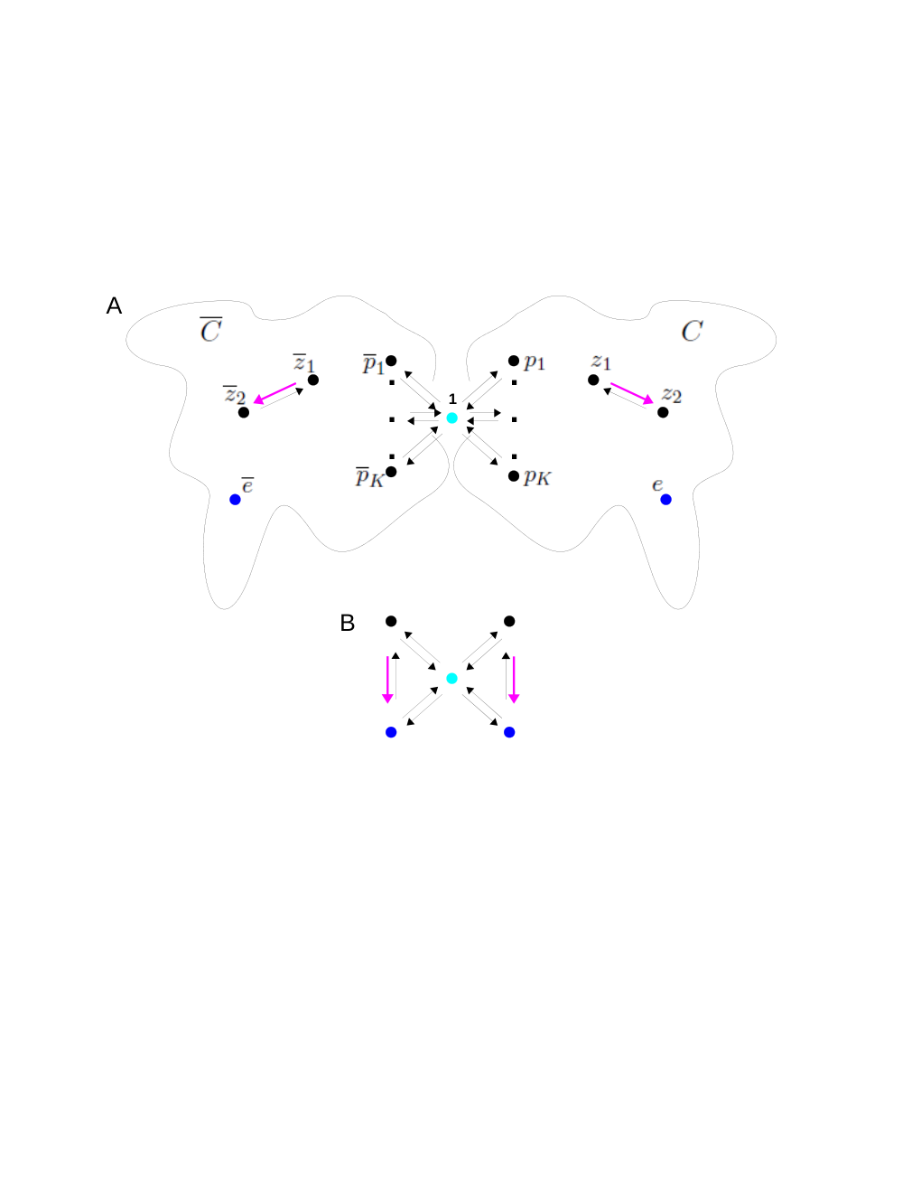
Hopfield’s analysis of discrimination between a correct and incorrect substrate sought to explain the low error rates in RNA and DNA synthesis [34]. Here, we analyse a general mechanism of Hopfield discrimination using the linear framework approach of [31]. Fig.2A shows a butterfly graph, $G=\overline{C}\bowtie C$, consisting of two “wings”, $\overline{C}$ and $C$, sharing a common reference vertex, $1$, (cyan). If $C$ and $\overline{C}$ are strongly connected, so too is $G$, and [31],

$$\rho_{i}(G)=\left\{\begin{array}[]{ll}\rho_{i}(\overline{C})\rho_{1}(C)&\mbox{if $i\in\overline{C}$}\\ \rho_{1}(\overline{C})\rho_{i}(C)&\mbox{if $i\in C$}\,.\end{array}\right.$$

(13)

For Hopfield discrimination, $C$ represents the mesostates interacting with the correct substrate and $\overline{C}$ the same for the incorrect substrate. Structurally (ie: ignoring labels), $C$ and $\overline{C}$ are mirror images of each other. Using overlines to map graph entities in $C$ to their mirror images in $\overline{C}$, $i\rightarrow j$ if, and only if, $\overline{i}\rightarrow\overline{j}$. $C$ is assumed to be reversible and strongly connected but otherwise arbitrary. Ligand binding to vertex $1$ leads to $K$ proximal vertices, $p_{1},\cdots,p_{K}$ and ligand is selected to be correct at a distinguished exit vertex, $e\not=1$. The error ratio is,

$$\varepsilon=\frac{u^{*}_{\overline{e}}(G)}{u^{*}_{e}(G)}=\frac{\rho_{\overline{e}}(\overline{C})\rho_{1}(C)}{\rho_{1}(\overline{C})\rho_{e}(C)}\,.$$

(14)

where the second equality comes from Eqs.4 and 13. Assume to begin with that $G$ is at thermodynamic equilibrium with labels $\ell_{eq}(i\rightarrow j)$. Following Hopfield, discrimination only takes place through unbinding from proximal vertices. Accordingly, $\ell_{eq}(i\rightarrow j)=\ell_{eq}(\overline{i}\rightarrow\overline{j})$ as long as $j\not=1$ and $\ell_{eq}(\overline{p}_{u}\rightarrow 1)=\alpha\ell_{eq}(p_{u}\rightarrow 1)$, where $\alpha>1$, so that the incorrect substrate has a higher off rate. Using Eq.6, it follows that the equilibrium error ratio is $\varepsilon_{eq}=\alpha^{-1}$. Accordingly, $\varepsilon_{eq}<1$.

Hopfield’s insight was that $\varepsilon_{eq}$ is independent of the number of discriminations, $K$, and the only way to exceed this “Hopfield barrier” [26] is to expend energy. He analysed the graph in Fig.2B, for which $K=2$ and $C$ has only three vertices, with energy expenditure on the magenta edge, and identified a parametric region for kinetic proofreading in which $(\varepsilon_{eq})^{2}<\varepsilon<\varepsilon_{eq}$ [34, 31]. The question we ask is what determines $\varepsilon$ when $K>2$ and $C$ is a general graph (Fig.2A) in which energy is expended at only a single energetic edge (magenta) where $\ell(z_{1}\rightarrow z_{2})=m\ell_{eq}(z_{1}\rightarrow z_{2})$.

We calculate how $\varepsilon$ depends on $m$ and $\alpha$ by exploiting the reformulation above, with Eq.7 being more convenient for this purpose than Eq.8, and by partitioning trees according to proximal edges (ie: edges $j\rightarrow 1$, where $j$ is a proximal vertex). We give a sketch here, with details in the Materials and Methods (M & M).

Given a polynomial ${\cal P}$ in the edge labels, we say that it is $m$-free, respectively $\alpha$-free, if $m$, respectively $\alpha$, does not divide any monomial in ${\cal P}$. Let $\Theta=\Theta_{1}(C)$. Eq.7 leads us to partition $\Theta$ according to the combinatorics of the energetic edge on minimal paths in $M(e,1)$,

$$\begin{array}[]{lcl}\Theta_{0}&=&\{T\in\Theta\,|\,z_{1}\rightarrow z_{2},z_{2}\rightarrow z_{1}\not\in T_{e}\}\\ \Theta_{+}&=&\{T\in\Theta\,|\,z_{2}\rightarrow z_{1}\in T_{e}\}\\ \Theta_{-}&=&\{T\in\Theta\,|\,z_{1}\rightarrow z_{2}\in T_{e}\}\,.\end{array}$$

(15)

Let $P_{0},P_{+},P_{-}\in M(e,1)$ be any choices of minimal paths arising as $T_{e}$ for $T\in\Theta_{0},\Theta_{+},\Theta_{-}$, respectively. By construction, different choices are energetically similar, so that $S(P_{0}),S(P_{+}),S(P_{-})$ are well defined for any choices of minimal paths. Furthermore, by Eq.12, $S(P_{+})=S(P_{0})-\ln(m)$, $S(P_{-})=S(P_{0})+\ln(m)$. Let us extend $q$ to subsets $X\subseteq\Theta$ by defining $q(X)=\sum_{T\in X}q(T)$ and note that $q_{eq}$ corresponds to $m=1$. We see from Eq.15 that $q(\Theta_{+})$ is $m$-free and that $q(\Theta_{-})=m\,q_{eq}(\Theta_{-})$. Hence we can rewrite Eq.7 as,

$$\rho_{e}(C)=\exp(-S(P_{0}))\left(q(\Theta_{0})+m\,q(\Theta_{+})+q_{eq}(\Theta_{-})\right)\,,$$

(16)

where $q(\Theta_{0})$ and $q_{eq}(\Theta_{-})$ are $m$-free but $q(\Theta_{0})$ may not be. The three parts of Eq.16, which come from the tripartite combinatorics of Eq.15, reflect the presence of only a single energetic edge.

We now introduce the partitioning scheme. Given $X\subseteq\Theta$, let $X^{(j,u)}\subseteq X$, for $1\leq j\leq K$ and $0\leq u\leq 1$, consist of those trees in $X$ with exactly $j$ proximal edges to $1$ and exactly $u$ energetic edges. The $X^{(j,u)}$ form a partition of $X$ into mutually disjoint subsets, so that $q(X)=\sum_{j,u}q(X^{(j,u)})$. By construction, $q(X^{(j,0)})$ is $m$-free and $q(X^{(j,1)})=m\,q_{eq}(X^{(j,1)})$, where $q_{eq}(X^{(j,1)})$ is $m$-free. Most importantly, again by construction,

$$q(\overline{X}^{(j,u)})=\alpha^{j}q(X^{(j,u)})\,,$$

(17)

where, evidently, $q(X^{(j,u)})$ is $\alpha$-free.

Eqs.16 and 17 make it straightforward to calculate the error ratio from Eq.14,

$$\varepsilon=\varepsilon_{eq}\left(\frac{(\overline{P}m+\overline{Q})(Rm+S)}{(\overline{R}m+\overline{S})(Pm+Q)}\right)\,,$$

(18)

where the eight coefficients in Eq.18, which are all $m$-free, are expressed in terms of the constructions above in Eq.30. It is striking that Eq.18 has the same algebraic form for the general graph in Fig.1A as for Hopfield’s simple graph in Fig.1B [31, Eq.4], albeit with vastly more complicated coefficients. The overlined coefficients in Eq.18 are each of degree $K$ in $\alpha=\varepsilon_{eq}^{-1}$, so that $\varepsilon$ is a rational function of $\varepsilon_{eq}$ and $m$. Eq.18 enables us to analyse discrimination in complex graphs (below).

Murugan et al, using Schnakenberg’s version of Eq.3, showed the rational dependence of $\varepsilon$ on $\varepsilon_{eq}$ [14, Eq.10]. Their treatment was based on a network similar to the butterfly graph in Fig.2A, with certain structural restrictions—the number of edges leaving the reference vertex equals the number entering the exit vertex—but allows for discriminations at non-proximal edges and global energy expenditure [14, Fig.3]. In view of the latter, they were unable to find an expression for $\varepsilon$, as we have in Eq.18. They did observe the following bounds on $\varepsilon$,

$$(\varepsilon_{eq})^{K}<\varepsilon<(\varepsilon_{eq})^{2-K}\,,$$

(19)

where the quantity corresponding to our $K$ is the number of “discriminatory edges” [14, C(i)]. Eq.19 is easy to deduce from Eq.18. The left-hand inequality in Eq.19 generalises Hopfield’s finding for Fig.1B with $K=2$. As noted by Murugan et al, Eq.19 allows for “anti-proofreading” regimes, where energy expenditure worsens the error ratio above the equilibrium value [14]. Indeed, this is already seen in the quadratic dependency of $\varepsilon$ on $m$ in Eq.18 [31].

There have been other studies of discrimination in addition to [14]. We have already drawn on [31] for the butterfly graph in Fig.2A. This work developed an asymptotic approach to the tradeoff between accuracy and speed of discrimination. Ehrenberg and colleagues [36, 37] and Savageau and colleagues [38, 39] rigorously analysed Hopfield’s remarks on multi-stage proofreading schemes [34]. In our language, they vertically extended the graph in Fig.2B to have multiple triangular “stages”. These studies established conditions for minimising energy expenditure for a given error ratio. Murugan et al, along with the results noted above, also analysed the accuracy-speed tradeoff [40, 14], finding multiple proofreading regimes in general networks similar to the butterfly graph in Fig.2A. They stated that optimal discrimination, for which $(\varepsilon_{eq})^{K}<\varepsilon<(\varepsilon_{eq})^{K-1}$, can be achieved in such networks for appropriate parameter choices [40, Eq.3]. An important distinction between these studies is that Murugan et al allow energy expenditure anywhere in the network, while Ehrenberg et al and Savageau et al allow energy expenditure at only one transition, as we have done above. We were therefore interested to know whether optimal discrimination is still possible in complex graphs with only a single energetic edge.

We found that the answer is yes. For example, consider the graph in Fig.3A. We note that this graph does not meet the structural restrictions mentioned above for the networks studied by Murugan et al in [40, 14]. We exploited the error ratio formula in Eq.18 to identify sets of parameter values for which this graph exhibits optimal discrimination, as detailed in Fig.3B (M & M). Such discrimination requires that each proximal edge contributes in a synergistic manner to the reduction in error, despite energy being expended at only a single edge which is distant in the graph. This synergy presumably arises from the global dependence of steady-state probabilities on all edge labels. It suggests remarkable global functional capabilities, despite only local energy expenditure, when the right parametric conditions are satisfied. It remains an intriguing problem to determine when optimal discrimination occurs and we hope to report on this subsequently.

We have studied Hopfield discrimination under the assumption of a single energetic edge. This relies, however, on the prior choice of a state of thermodynamic equilibrium. Moreover, energy expenditure could also occur not simply at one edge but through coupling at multiple edges to reservoirs with different chemical potentials, as happens during enzymatic catalysis. It is important, therefore, to have a more independent and flexible means to exploit the reformulation in Eq.8. In the spirit of Schnakenberg, [3], we consider any basis, $B$, of oriented minimal cycles, $B=\{B_{1},\cdots,B_{q}\}$. Such a basis arises by choosing a spanning tree and adjoining an edge outside the tree to create each minimal cycle, for which an arbitrary orientation is chosen (M & M). The number, $q$, of minimal cycles in any basis is the Betti number of $G$, $\beta_{1}(G)$, or the rank of the first homology group of $G$ considered as a topological space. Let $\iota(B)$ denote the number of cycles $B_{i}$ which break the cycle condition, $\iota(B)=\#i\,,1\leq i\leq q\,,S(B_{i})\not=0$. We define the entropy production index of the graph $G$, $\iota(G)$, to be the minimum of these quantities over all cycle bases, $\iota(G)=\min_{B}\iota(B)$. Evidently, $0\leq\iota(G)\leq\beta_{1}(G)$. The case $\iota(G)=0$ corresponds to thermodynamic equilibrium. It is not difficult to show that $\iota(G)=1$ corresponds to the case considered here, and also in [36, 37, 38, 39], of a single energetic edge (M & M). The case considered in [40, 14] corresponds to the entropy production index being maximal, $\iota(G)=\beta_{1}(G)$. The quantity $\iota(G)$, which is thermodynamic in the language of Maes [41] (below), offers a first step in partitioning the non-equilibrium landscape.

Recall the partitioning scheme introduced above in which a subset of spanning trees rooted at the reference vertex, $X\subseteq\Theta$, is divided into parts, $X^{(j,u)}$, for $1\leq j\leq K$ and $0\leq u\leq 1$. $X^{(j,u)}$ consists of those trees in $X$ with exactly $j$ proximal edges to $1$ and exactly $u$ energetic edges. In other words, $T\in X^{(j,u)}$ if, and only if, there are distinct proximal vertices, $p_{i_{1}},\cdots,p_{i_{j}}$ in $C$, which may depend on $T$, such that $p_{i_{1}}\rightarrow 1,\cdots,p_{i_{j}}\rightarrow 1\in T$ but no other proximal vertices have this property; and, if $u=0$, $z_{1}\rightarrow z_{2}\not\in T$, while if $u=1$, $z_{1}\rightarrow z_{2}\in T$. Note that any tree in $\Theta$ must have between $1$ and $K$ proximal edges to $1$ and no more than $1$ energetic edge (Fig.2A). It follows that the $X^{(j,u)}$ form a partition of $X$ into disjoint subsets,

$$X=(X^{(1,0)}\amalg X^{(1,1)})\amalg\cdots\amalg(X^{(K,0)}\amalg X^{(K,1)})\,.$$

(20)

Hence, we can decompose $q(X)$ as follows,

$$\begin{split}q(X)&=\left(q(X^{(1,0)})+\cdots+q(X^{(K,0)})\right)\\ &+m\left(q_{eq}(X^{(1,1)})+\cdots+q_{eq}(X^{(K,1)})\right)\end{split}$$

(21)

where the terms $q(X^{(j,0)})$ and $q_{eq}(X^{(j,1)})$ are all $m$-free. The value of this decomposition becomes clear by applying Eq.17 to see that,

$$\begin{split}q(\overline{X})&=\left(\alpha q(X^{(1,0)})+\cdots+\alpha^{K}q(X^{(K,0)})\right)\\ &+m\left(\alpha q_{eq}(X^{(1,1)})+\cdots+\alpha^{K}q_{eq}(X^{(K,1)})\right)\,,\end{split}$$

(22)

where the expressions $q(X^{(j,0)})$ and $q_{eq}(X^{(j,1)})$ are both $m$-free, as above, and, by construction, $\alpha$-free.

Let us abbreviate $\sum_{1\leq j\leq K}$ by $\sum_{j}$. Since $\rho_{1}(C)=q(\Theta)$, it follows from Eq.21 that,

$$\rho_{1}(C)=\left(\sum_{j}q(\Theta^{(j,0)})\right)+m\left(\sum_{j}q_{eq}(\Theta^{(j,1)})\right)\,.$$

(23)

Similarly, applying Eq.22 to $\rho_{1}(\overline{C})=q(\overline{\Theta})$, we see that,

$$\rho_{1}(\overline{C})=\left(\sum_{j}\alpha^{j}q(\Theta^{(j,0)})\right)+m\left(\sum_{j}\alpha^{j}q_{eq}(\Theta^{(j,1)})\right)\,.$$

(24)

We begin with Eq.16 which represented $\rho_{e}(C)$ in terms of a partition into disjoint subsets of $\Theta$,

$$\Theta=\Theta_{0}\amalg\Theta_{+}\amalg\Theta_{-}\\$$

(25)

It is clear from Eq.16 that, for all $1\leq j\leq K$,

$$\Theta_{+}^{(j,1)}=\emptyset\hskip 5.0pt\mbox{and}\hskip 5.0pt\Theta_{-}^{(j,0)}=\emptyset\,.$$

(26)

If we now apply the decomposition in Eq.21 to each of the three subsets of Eq.25, and collect together the $m$-free terms in Eq.16, we find that,

$$\begin{array}[]{c}\rho_{e}(C)=\exp(-S(P_{0}))\,\,\times\\ \left[\sum_{j}\left(q(\Theta_{0}^{(j,0)})+q_{eq}(\Theta_{-}^{(j,1)})\right)\right.\\ +\left.m\left(\sum_{j}\left(q_{eq}(\Theta_{0}^{(j,1)})+q(\Theta_{+}^{(j,0)})\right)\right)\right]\,.\end{array}$$

(27)

Similarly, using the decomposition in Eq.22, we find that,

$$\begin{array}[]{c}\rho_{\overline{e}}(\overline{C})=\alpha^{-1}\exp(-S(P_{0}))\,\,\times\\ \left[\sum_{j}\alpha^{j}\left(q(\Theta_{0}^{(j,0)})+q_{eq}(\Theta_{-}^{(j,1)})\right)\right.\\ +\left.m\left(\sum_{j}\alpha^{j}\left(q_{eq}(\Theta_{0}^{(j,1)})+q(\Theta_{+}^{(j,0)})\right)\right)\right]\,,\end{array}$$

(28)

where we have used the fact that $S(\overline{P_{0}})=\alpha^{-1}S(P_{0})$.

We have now calculated each of the four terms appearing in Eq.18. Using overlines again to indicate coefficients from the mirror image subgraph $\overline{C}$ and recalling that $\alpha=(\varepsilon_{eq})^{-1}$, we find that,

$$\varepsilon=\varepsilon_{eq}\left(\frac{(\overline{P}m+\overline{Q})(Rm+S)}{(\overline{R}m+\overline{S})(Pm+Q)}\right)\,.$$

(29)

The eight coefficients in Eq.29 are given by

$$\begin{array}[]{lcl}P&=&\sum_{j}q_{eq}(\Theta_{0}^{(j,1)})+q(\Theta_{+}^{(j,0)})\\ Q&=&\sum_{j}q(\Theta_{0}^{(j,0)})+q_{eq}(\Theta_{-}^{(j,1)})\\ R&=&\sum_{j}q_{eq}(\Theta^{(j,1)})\\ S&=&\sum_{j}q(\Theta^{(j,0)})\\ \overline{P}&=&\sum_{j}\alpha^{j}(q_{eq}(\Theta_{0}^{(j,1)})+q(\Theta_{+}^{(j,0)}))\\ \overline{Q}&=&\sum_{j}\alpha^{j}(q(\Theta_{0}^{(j,0)})+q_{eq}(\Theta_{-}^{(j,1)}))\\ \overline{R}&=&\sum_{j}\alpha^{j}q_{eq}(\Theta^{(j,1)})\\ \overline{S}&=&\sum_{j}\alpha^{j}q(\Theta^{(j,0)})\,.\end{array}$$

(30)

The various expressions of the form $q(-)$ or $q_{eq}(-)$ in Eq.30 are all both $\alpha$-free and $m$-free. Eqs.29 and 30 establish Eq.18.

Using the fact that $\alpha>1$, which encodes the distinction between the correct and incorrect substrate, we see by inspection of Eq.30, that

$$\begin{array}[]{rcccl}\alpha(P+Q)&<&\overline{P}+\overline{Q}&<&\alpha^{K}(P+Q)\\ \alpha(R+S)&<&\overline{R}+\overline{S}&<&\alpha^{K}(R+S)\,.\end{array}$$

It follows that

$$\alpha<\frac{\overline{P}+\overline{Q}}{P+Q}<\alpha^{K}$$

(31)

and also that

$$\alpha^{-K}<\frac{R+S}{\overline{R}+\overline{S}}<\alpha^{-1}$$

(32)

Combining Eqs.31 and 32 and using Eq.29 and the fact that $\alpha=(\varepsilon_{eq})^{-1}$, we see that,

$$(\varepsilon_{eq})^{K}<\varepsilon<(\varepsilon_{eq})^{2-K}\,,$$

(33)

which proves Eq.19.

Eq.18 expresses $\varepsilon$ as a quadratic rational function of $m$. This graph of this function can exhibit many shapes [31] and we looked for the conditions under which it has a positive minimum, which implies proofreading. The derivative, $d\varepsilon/dm$, has a quadratic numerator and it is readily seen that $\varepsilon$ is decreasing at $m=0$ if,

$$\frac{S\overline{P}+R\overline{Q}}{P\overline{S}+Q\overline{R}}<\frac{S\overline{Q}}{Q\overline{S}}\,.$$

(34)

When Eq.34 holds, $\varepsilon$ has a single positive minimum if also,

$$\frac{S\overline{P}+R\overline{Q}}{P\overline{S}+Q\overline{R}}<\frac{R\overline{P}}{P\overline{R}}\,.$$

(35)

We sought this minimum error ratio for the graph in Fig.3A. First, an independent set of edge labels were chosen using a spanning tree, as previously described [26]. Numerical values for these rates on the correct wing of the graph, $C$, were chosen independently as $10^{x}$, where $x$ was drawn randomly from the uniform distribution on $[-3,+3]$. The remaining edge labels, not on the spanning tree, which determine independent cycles, were chosen to make $\iota(G)=0$, so that $G$ is at thermodynamic equilibrium. The labels on the incorrect wing, $\overline{C}$, were then determined by the relationships described in the main text. The value of $\alpha$, which gives the equilibrium error ratio, $\varepsilon_{eq}=\alpha^{-1}$, was arbitrarily set to $0.1$. Departure from thermodynamic equilibrium was imposed through the multiplier, $m$, on the energetic edge, $\ell(z_{1}\rightarrow z_{2})=m\ell_{eq}(z_{1}\rightarrow z_{2})$, while all other edge labels kept their previously assigned values, $\ell(i\rightarrow j)=\ell_{eq}(i\rightarrow j)$ when $i\not=z_{1}$ or $j\not=z_{2}$. Spanning trees were enumerated using Matlab’s generateSpanningTrees function and the eight coefficients, $P,Q,R,S,\overline{P},\overline{Q},\overline{R},\overline{S}$ in Eq.18 were numerically calculated from Eq.30. If they did not satisfy the inequalities in Eqs.34 and 35, the parameter set was rejected. If they did, the value of $m$ giving the positive minimum of $\varepsilon$ was calculated from the quadratic numerator of $d\varepsilon/dm$ as,

$$m_{*}=\frac{P\overline{Q}S\overline{R}-Q\overline{P}R\overline{S}+\sqrt{(P\overline{Q}-Q\overline{P})(SP-QR)(\overline{S}\overline{P}-\overline{Q}\overline{R})(R\overline{S}-S\overline{R})}}{R\overline{P}(P\overline{S}+Q\overline{R})-P\overline{R}(S\overline{P}+R\overline{Q})}\,,$$

and the corresponding minimum value of $\varepsilon$ was determined by substituting $m_{*}$ into Eq.18. $\sim\!\!10^{7}$ parameter sets were sampled, of which $\sim\!\!1.2\times 10^{5}$ had minimum error ratios satisfying $\ln(\varepsilon)/\ln(\varepsilon_{eq})>1.4$, as reported in Fig.3B.

References

- [1] Hill TL (1966) Studies in irreversible thermodynamics IV. Diagrammatic representation of steady state fluxes for unimolecular systems. J. Theoret. Biol. 10:442–59.
- [2] Hill TL (2004) Free Energy Transduction and Biochemical Cycle Kinetics. (Dover Publications, New York, USA).
- [3] Schnakenberg J (1976) Network theory of microscopic and macroscopic behaviour of master equation systems. Rev. Mod. Phys. 48:571–86.
- [4] Evans DJ, Cohen EGD, Morriss GP (1993) Probability of second law violations in shearing steady states. Phys. Rev. Lett. 71:2401–4.
- [5] Gallavotti G, Cohen EGD (1995) Dynamical ensembles in nonequilibrium statistical mechanics. Phys. Rev. Lett. 74:2694–7.
- [6] Jarzynski C (1997) Equilibrium free-energy differences from non-equilibrium measurements: a master equation approach. Phys. Rev. E 56:5018–35.
- [7] Kurchan J (1998) Fluctuation theorem for stochastic dynamics. J. Phys. A: Math. Gen. 31:3719–29.
- [8] Lebowitz JL, Spohn H (1999) A Gallavotti–Cohen-type symmetry in the large deviation functional for stochastic dynamics. J. Stat. Phys. 95:333–65.
- [9] Maes C (1999) The fluctuation theorem as a Gibbs property. J. Stat. Phys. 95:367–92.
- [10] Crooks GE (1999) Entropy production fluctuation theorem and the nonequilibrium work relation for free energy differences. Phys. Rev. E 60:2721–6.
- [11] Seifert U (2008) Stochastic thermodynamics: principles and perspectives. Eur. Phys. J. B 64:423–31.
- [12] Andrieux D, Gaspard P (2007) Fluctuation theorem for currents and Schnakenberg network theory. J. Stat. Phys. 127:107–31.
- [13] Maes C, Netočný K (2013) Heat bounds and the Blowtorch Theorem. Ann. Henri Poincaré 14:1193–202.
- [14] Murugan A, Huse DA, Leibler S (2014) Discriminatory proofreading regimes in nonequilibrium systems. Phys. Rev. X 4:021016.
- [15] Ventsel’ AD, Freidlin MI (1970) On small random dynamical perturbations of dynamical systems. Russ. Math. Surv. 25:1–54.
- [16] Freidlin MI, Wentzell AD (2012) Random perturbations of dynamical systems. (Springer, Heidleberg, Germany), 3 edition.
- [17] Wales DJ (2006) Energy landscapes: calculating pathways and rates. Int. Rev. Phys. Chem. 25:237–82.
- [18] Cameron M, Vanden-Eijnden E (2014) Flows in complex networks: theory, algorithms, and application to Lennard-Jones cluster rearrangement. J. Stat. Phys. 156:427–54.
- [19] Gunawardena J (2012) A linear framework for time-scale separation in nonlinear biochemical systems. PLoS ONE 7:e36321.
- [20] Mirzaev I, Gunawardena J (2013) Laplacian dynamics on general graphs. Bull. Math. Biol. 75:2118–49.
- [21] Mirzaev I, Bortz DM (2015) Laplacian dynamics with synthesis and degradation. Bull. Math. Biol. 77:1013–45.
- [22] Yordanov P, Stelling J (2018) Steady-state differential dose response in biological systems. Biophys. J. 114:723–36.
- [23] Yordanov P, Stelling J (2020) Efficient manipulation and generation of Kirchhoff polynomials for the analysis of non-equilibrium biochemical reaction networks. J. Roy. Soc. Interface 17:20190828.
- [24] Dasgupta T, et al. (2014) A fundamental trade off in covalent switching and its circumvention by enzyme bifunctionality in glucose homeostasis. J. Biol. Chem. 289:13010–25.
- [25] Nam KM, Gyori BM, Amethyst SV, Bates DJ, Gunawardena J (2020) Robustness and parameter geography in post-translational modification systems. PLoS Comp. Biol. 16:e1007573.
- [26] Estrada J, Wong F, DePace A, Gunawardena J (2016) Information integration and energy expenditure in gene regulation. Cell 166:234–44.
- [27] Biddle JW, Nguyen M, Gunawardena J (2019) Negative reciprocity, not ordered assembly, underlies the interaction of Sox2 and Oct4 on DNA. eLife 8:e410172018.
- [28] Wong F, Dutta A, Chowdhury D, Gunawardena J (2018) Structural conditions on complex networks for the Michaelis-Menten input-output response. Proc. Natl. Acad. Sci. USA 115:9738–43.
- [29] Park J, et al. (2019) Dissecting the sharp response of a canonical developmental enhancer reveals multiple sources of cooperativity. eLife 8:e41266.
- [30] Wong F, Gunawardena J (2020) Gene regulation in and out of equilibrium. Annu. Rev. Biophys. 49:199–226.
- [31] Wong F, Amir A, Gunawardena J (2018) Energy-speed-accuracy relation in complex networks for biological discrimination. Phys. Rev. E. 98:012420.
- [32] Kirchhoff G (1847) Ueber der Auflösung der Gleichungen, auf welche man bei Untersuchung der linearen Vertheilung galvanischer Ströme geführt wird. Annalen der Physik und Chemi 72:497–508.
- [33] Tutte WT (1948) The dissection of equilateral triangles into equilateral triangles. Proc. Camb. Phil. Soc. 44:463–82.
- [34] Hopfield JJ (1974) Kinetic proofreading: a new mechanism for reducing errors in biosynthetic processes requiring high specificity. Proc. Natl. Acad. Sci. USA 71:4135–39.
- [35] Bauer M, Cornu F (2015) Local detailed balance: a microscopic derivation. J. Phys. A: Math. Theor. 48:015008.
- [36] Ehrenberg M, Blomberg C (1980) Thermodynamic constraints on kinetic proofreading in biosynthetic pathways. Biophys. J. 31:333–58.
- [37] Blomberg C, Ehrenberg M (1981) Energy considerations for kinetic proofreading in biosynthesis. J. Theor. Biol. 88:631–70.
- [38] Freter RR, Savageau MA (1980) Proofreading systems of multiple stages for improved accuracy of biological discrimination. J. Theor. Biol. 85:99–123.
- [39] Savageau MA, Lapointe DS (1981) Optimization of kinetic proofreading: a general method for derivation of the constraint relations and an exploration of a specific case. J. Theor. Biol. 93:157–77.
- [40] Murugan A, Huse DA, Leibler S (2012) Speed, dissipation, and error in kinetic proofreading. Proc. Natl. Acad. Sci. USA 109:12034–9.
- [41] Maes C (2020) Frenesy: time-symmetric dynamical activity in nonequilibria. Physics Reports 850:1–33.
- [42] Crocker J, et al. (2015) Low affinity binding site clusters confer Hox specificity and regulatory robustness. Cell 160:191–203.
- [43] Komatsu TS, Nakagawa N (2008) Expression for the stationary distribution in nonequilibrium steady states. Phys. Rev. Lett. 100:030601.
- [44] Maes C, Netočný K, Wynants B (2008) On and beyond entropy production: the case of Markov jump processes. Markov Process. Relat. 14:445–64.
- [45] Broder A (1989) Generating random spanning trees in Proceedings 30th IEEE Symposium on Foundations of Computer Science. pp. 442–7.
- [46] Aldous D (1990) The random walk construction of uniform spanning trees and uniform labelled trees. SIAM J. Discrete Math. 3:450–65.
- [47] Wilson DB (1996) Generating random spanning trees more quickly than the cover time in Proceedings 28th Annual ACM Symposium on Theory of Computing. pp. 296–303.
- [48] Pitman J, Tang W (2018) Tree formulas, mean first passage times and Kemeny’s constant of a Markov chain. Bernoulli 24:1942–72.
- [49] Landauer R (1975) Inadequacy of entropy and entropy derivatives in characterizing the steady state. Phys. Rev. A 12:636–8.
- [50] Jaynes ET (1957) Information theory and statistical mechanics. Phys. Review 106:620–30.
- [51] Prigogine I (1967) Introduction to Thermodyanmics of Irreversible Processes. (Interscience, New York, USA).
- [52] Feynman RP (1948) Space-time approach to non-relativistic quantum mechanics. Rev. Mod. Phys. 20:367.
- [53] Crooks GE (2000) Path-ensemble averages in systems driven far from equilibrium. Phys. Rev. E 61:2361–6.