Efficient quantum memory for heralded single photons generated by cavity-enhanced spontaneous parametric downconversionPreprint: APS/123-QED
Abstract
We interface a spontaneous parametric down conversion (SPDC) crystal and a cold atomic ensemble and demonstrate a highly efficient quantum memory through polarization-encoded single-photon qubits. Specifically, narrowband heralded single photons from a cavity-enhanced SPDC source is stored using cold atomic ensemble, with storage-and-retrieval efficiency and storage time at efficiency. To prevent the degradation after storage, we also manipulate the single-photon wave profile so that the retrieved non-classical nature of single photon is preserved. On the other hand, the dual-rail storage is used for storing polarization-encoded qubits, and the corrected fidelity of flying qubits after storage reaches . The results pave the way toward large-scale quantum network.
I Introduction
Quantum networks relies on efficient transfer between flying qubits and stationary quantum nodes Kimble 2008; Cao et al. 2020. To facilitate the distribution of entanglement over large-scale network, the synchronization between two distant nodes are essential for many protocols, such as quantum repeaters Sangouard et al. 2011, linear optics quantum computation (LOQC) Knill et al. 2001. To do that, quantum memories, devices that can store and retrieve flying qubits on demand, are critical tools. Thus, intensive efforts have been made on optical storage with promising results, such as storage efficiency (SE) with electromagnetically induced transparency (EIT) Hsiao et al. 2018, with off resonance Raman interaction Reim et al. 2010, with photon echo technique Hedges et al. 2010, and with Autler-Townes-splitting protocol (ATS) Saglamyurek et al. 2018. However, most of them are working on attenuated or single-photon-level coherent light. It should be pointed out that although some protocols can be realised through single-photon-level classical light source, developing single-photon Fock state is essential for a wider range of applications on quantum information processing, such as LOQC Knill et al. 2001 and entanglement transferWootters 1998; Cao et al. 2020. While fewer works have addressed quantum storage for single photons, pushing toward universal quantum networks remains challenging.
To generate single photon, the possible platforms include single atoms inside a cavity McKeever et al. 2004, four-wave mixing from the cold atomic ensemble Du et al. 2008, NV (nitrogen-vacancy) centers in diamond Bahe et al. 2009; Sipahigil et al. 2012, the Duan–Lukin–Cirac–Zoller protocol (DLCZ) by cold atomic ensembles Duan et al. 2001; Cao et al. 2020. The merit of cold-atom-based single photon source is that the central frequencies match the atomic transitions, and photons are inherently narrow-band, which enables the stronger interaction and yields higher efficiency. Up to date, works toward highly efficient quantum storage of cold-atom-generated single photon have been demonstrated with SE , the fidelityWang et al. 2019, and with SE and preserving antibunching nature Cao et al. 2020. Yet, the tedious setup for atom-based photon source is relatively arduous to scale up, which is difficult for more sophisticated manipulation on flying qubits.
Conversely, spontaneous parametric down conversion (SPDC) crystals, one of the most widely used photonic entanglement sources, are suitable for large-scale protocols Tsai et al. 2020. The drawbacks of them are ultra-broad bandwiths (THz), hindering the direct interaction with atoms. The issue can be solved elegantly through placing crystals into high-fitness optical cavities, suppressing the spectral linewidths of single photons to MHz level without sacrificing photons Tsai and Chen 2018; Zhang et al. 2011. Nevertheless, although the quantum storage of SPDC-based photon sources have been realize Tsai et al. 2020; Zhang et al. 2011; Akiba et al. 2009; Clausen et al. 2011; Seri et al. 2018; Seri et al. 2019; Rieländer et al. 2014, the SEs are typically low. The best SE is Tsai et al. 2020 in previous works, which has not yet beat the no-cloning theorem limits Grosshans and Grangier 2001 and loss tolerance in cluster state computationVarnava et al. 2006. The major difficulties include noises pollution Wang et al. 2019 (see Appendix V.4), mode stabilization of SPDC crystals Tsai and Chen 2018. Many efforts have been made to generate bright, narrowband Tsai and Chen 2018, single-mode single photon sources Chuu and Harris 2011, in order to maximize the light-matter interaction and thus increase SE.
In this work, we demonstrate a highly efficient quantum memory with SE of SPDC photons, which to our knowledge is the best record for crystal-generated photon sources. As for quantum memories, the choice of cold atomic ensemble enables us to reach high storage efficiency and long storage times Hsiao et al. 2018. We aim to build a compact photon source for easily scaling up, while maintaining the efficient transfer between channels and a node. Such a setup allows us to conduct advanced manipulations on photonic states with large-scale photon sources, such as post-selected entanglements Bao et al. 2008; Scholz et al. 2009, and the generated photons can be efficiently stored and delivered using a cold atomic quantum memory. The crystal-atom-interfaced system forms a quantum node in a quantum network with more freedom to manipulate photonic states.
II Experimental Setup
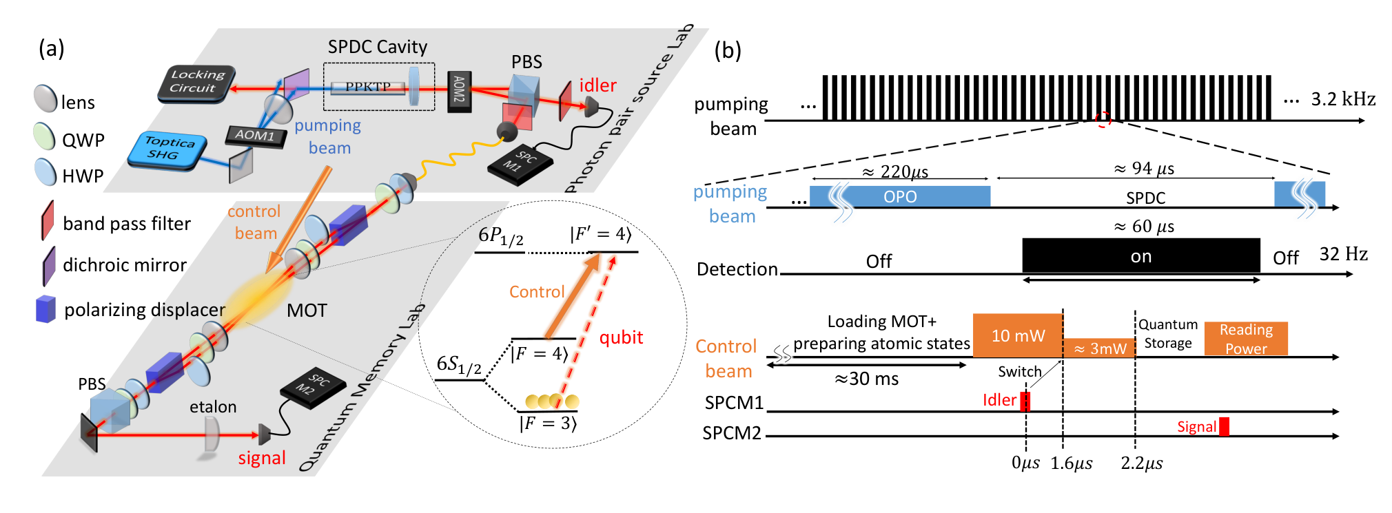
The experimental setup consists of a photon-pair source and a cold atom system, as shown in Fig.1a. The nondegenerate, narrowband photon pairs are generated from a cavity-enhanced SPDC setup with a single longitudinal mode. A Toptica frequency-doubling laser, which serves as the pump beam with a wavelength of 447 nm, pumps the type-II periodically poled KTiOPO4 (PPKTP) crystal in the high-finesse linear cavity. Due to the similar reflectivity of the mirrors on the two sides of the linear cavity, the down-converted photons travel nearly 50/50 forward and backward. During the experiment, the pump power alternates between a high-power () phase and a low-power phase with a switching rate of 3.2 kHz. duty cycle operates with the high-power phase, which is controlled by an acousto-optic modulator (AOM1) (see Fig.1 b). During the high-power phase (which is corresponding to the optical parametric oscillator, OPO), the backward beam provides the signal for cavity frequency stabilization. The forward beam is modulated by AOM2, which serves as an optical switch with the same driving frequency as AOM1. AOM2 is out of phase to AOM1 with a duty cycle. This allows the beam to pass only during the low-power phase (SPDC) and prevents the photon detectors (SPCM) from being damaged. Signal and idler photons are separated by a polarizing beam splitter (PBS) and are further sent to the cold-atom system and received as triggers, respectively. The linewidth of the heralded single photons is 2.2 MHz. The OPO output light is beating with a reference laser, of which the frequency is controlled by a double-passed AOM. The central frequency of the signal beam is locked at transition (895 nm) by locking the beat frequency to a certain value. More technical details can be referred to Tsai and Chen 2018.
A magneto-optical trap (MOT) of cesium with cigar-shaped atomic clouds is used to implement the quantum memory with electromagnetically induced transparency (EIT) protocol Tsai and Chen 2018; Hsiao et al. 2018. The EIT memory is operated at line, with the signal photons drive the to transition and the strong control field drives the to transition, as shown in the sub-graph of Fig.1 a. The choice of line allows us to reduce the control-intensity-dependent ground-state decoherence rate due to the off-resonant excitation of the control field to the nearby transition Hsiao et al. 2018; Tsai and Chen 2018. The temporally dark and compressed MOT and Zeeman-state optical pumping are used to increase the optical depth Hsiao et al. 2014. The achieved optical depth is when a MOT repetition rate set at Hz, respectively. The optical depth is determined by the EIT spectral fitting by setting the decay rate of the optical coherence () to be , where MHz is the linewidth of transition. This decay rate is larger than an ideal value of 0.5 (solely due to the spontaneous decay) because the contribution due to laser linewidth and laser frequency fluctuation is consideredHsiao et al. 2018.
The idler photons are detected by SPCM1 for heralding while signal photons are sent to the quantum memory laboratory through a m optical fiber, which is used to induce a s temporal delay. This optical delay is technically essential such that the optical switch for the control beam can response before the signal photons passing through the MOT cell. Then, the signal photons pass through the polarization displacer to map the polarizations of the qubit into the two spatial modes Vernaz-Gris et al. 2018; Wang et al. 2019. A half-wave plate is added in one of the spatial mode, such that both modes have the same polarization before interacting with cold atomic ensembles. Because the atomic population is optically pumped towards the rightmost Zeeman states to increase the optical depth, such a dual-rail setup allows us to store any polarization of flying qubits without lossing much of optical depthVernaz-Gris et al. 2018; Wang et al. 2019. Before coming into the MOT cell, the signal beam is focused by a lens to an intensity diameter of around the atomic clouds while the control beam is collimated with a diameter of . The angle between the signal and control beam is . This angle is carefully selected such that the noises from the control beam are minimized while the ground state decoherence rate is still suppressed at , which majorly comes from the residual Doppler broadening. After passing through the MOT cell, the signal beam passes a reverse setup as that before entering into the MOT cell, such that both spatial modes are collimated and combined. The signal photons are then collected by SPCM2 before passing four irises, two elatons (Quantaser FPE001), and a bandpass filter (Semrock FF01-900/25), which are all used to filter out the noises. The reduction of external noises is essential to preserve the quantum nature of the single photons, as discussed in Appendix.V.3. The overall collection efficiency, defined as the power ratio between that at the photon counter and the output right after SPDC, is .
Fig.1b depicts the time sequence of our experiment. The repetition rates for the photon pair source and MOT are 3.2 kHz and 32 (or 16) Hz, respectively. Within each MOT period, there is a for cold atoms loading and states preparation and then the MOT is turned off for ms. During the MOT off time, the photon-pair system is at the photon-pair mode for . Waiting for s to allow the leaking photons from the OPO phase to a negligible levelTsai et al. 2020, the latter time window is left for collecting data. Once the SPCM1 detects an idler photon, the electronic signal is sent to the optical switch, and the control beam is switched to an optimal intensity ( mW) for quantum storage Hsiao et al. 2018. Before that, the control beam is set to a stronger intensity ( mW) in order to clear out atomic population at the state (see Appendix.V.4). After the signal photons entering into the atomic ensemble, the control beam is ramp off to convert the signal photons into atomic spin-waves. After storing for a given time, the control beam is ramp up to retrieve the signal photons. The single photons are then collected by SPCM2 and record by an oscilloscope (RTO2014).
III results
III.1 Single-Photon Source

We first characterize the nonclassical property of the heralded single photons by measuring the normalized cross-correlation function , where and . In the experiment, the normalized cross-correlation function can be determined by , where is the probability of detecting the signal (idler) photons, and is the probability of detecting the coincidence events of both signal and idler photonsTsai et al. 2020. is determined by the bin width . If one assumes the second-order auto-correlations of signal and idler , manifests the violation of classical property Tsai and Chen 2018; Clausen et al. 2011; Kuzmich et al. 2003. Thus, it is desirable to pursue a better for enlarging the violation factor Tsai and Chen 2018. Therefore, we scan through the pump power to determine the best working point, as shown in Fig.2b. The detailed theory used to model the data can be referred to Appendix.V.3. At the best working point, the maximum are and right after the photon source and after arriving at quantum memory setup, respectively, as shown in Fig.2a.
The anti-bunching behavior of the single-photon nature is also confirmed by measuring the conditional second order autocorrelation function for the signal photons , which should be for an ideal single-photon Fock state and for coherent light. Our measured is after arriving at quantum memory setup, as shown in Fig.2c. More details can be referred to Appendix.V.1
III.2 Storage of Heralded Single Photons
We then conduct the experiment on storage of heralded single photons. The repetition rate of the experiment is set at Hz. We vary the control intensity during the retrieval process to manipulate the waveform and non-classical correlation of the retrieved signal photons. The data with a storage time of ns for various ratios between the reading to writing control intensity are shown in Fig.3a. It is evident that the peak height of the retrieved signal pulse is higher for a stronger reading control field. We emphasize that the implementation of EIT memory in line allows us to increase of signal photon without sacrificing the storage efficiency, compared to the case of transition. This is due to the significant reduction of the off-resonant coupling of the control field to the nearby transition for the line as compared to the Tsai et al. 2020; Hsiao et al. 2018. The peak and storage-and-retrieval efficiency (SE) versus the control intensity ratio (from 1-5.6) are depicted in Fig.3b and c, respectively. The details of the determination of the efficiency are described in Appendix.V.2. The efficiencies (SE) are around for different control intensity ratio. A slight deviation from the average efficiency for some data points may due to the drift of the system parameters (e. g. optical depth) since it takes hours for collecting each data set.
Although the peak height of the signal pulse is greater for a stronger control intensity ratio as shown in Fig.3a, the peak for the retrieved signal photons still saturate at higher intensity ratios as shown in Fig.3b. The peak increases by a factor of for ratio from 1 to 3.3. This means that one can manipulate the waveform (or bandwidth) and the non-classical correlation of the retrieved signal photons by the EIT memory through varying the writing control intensityTsai et al. 2020. The saturation of the peak at high writing control intensity is due to the increasing in the noise background which may come from the control leakage and Raman-induced noises. More discussions on the noises are shown in Appendix.V.4. In all cases, the peak are all larger than 2. Therefore, the non-classical property of the heralded single photons is preserved by the EIT memory. The highest retrieved peak reaches at .
Next, we measure the retrieved signal photons for various storage time, as shown in Fig.4 a. The peak and efficiency versus the storage time are analyzed in Fig.4 b and c, respectively. The efficiency is below at , while the drops to half of the value without storage at . The delay-bandwidth product (DBP), usually defined as the ratio of the storage time when efficiency is 50% to the FWHM duration of the input signal pulses, is an important figure of merit of the memory to quantify the ability to store the quantum nature. However, our work is the only one so far with an efficiency of larger than 50 % for storage of single photons generated by the SPDC source. In order to compare with other works, we adopt the definition of DBP as the product of the storage time when retrieved is 50% of its initial value with null storage time and the photon bandwidth. The comparison is shown in Fig.4 dHsiao et al. 2018; Chen et al. 2013; Wei et al. 2020. Although there is still a lot of room to improve our result, the achieved DBP of and the efficiency of 70% are the best among these works.
.
III.3 Storage of Polarization Qubits

A quantum memory should be able to store arbitrary states of qubit. We encode the polarization qubit into the heralded single photons by the dual-rail schemeVernaz-Gris et al. 2018; Wang et al. 2019, as shown in Fig.1a. The polarization of the signal photons is mapped into the spatial mode. For example, for a qubit with a quantum state , the dual-rail setup converts it into
| (1) |
where denote horizontal and vertical polarization; denote two different spatial modes (see Fig.1a). The reversed setup is used after the MOT cell for mapping the spatial modes back into the original polarization states. We then use a set of wave-plates and polarization beam splitters to perform the quantum state tomographyJames et al. 2001. The repetition rate of the experiment is set to Hz to speed up the data collection.
Figures 5a-d depict the reconstructed density matrices of the retrieved signal photons, of which the initial polarization states are and , respectively. The average fidelity reaches . The performance is mainly limited by the low heralding efficiency () and the background noises. Note that our mean photon number is per heralded event, so the requirement on noises is very demanding Vernaz-Gris et al. 2018. By subtracting the background noises, the average corrected fidelity is (see Fig.5). The average storage efficiency is . Compared with the single-rail setup, the possible reasons for the reduced efficiency are described below. First, the optical depth is reduced from to due to operating the experiment at a higher repetition rate (from 16 to 32 Hz), which is not favorable for a high efficiency. Second, the two spatial modes of the signal photons have a certain separation (mm) such that the experienced optical depth may be reduced. In addition, the size of the control beam is not large enough to cover the two signal modes around its peak intensity region. The in-homogeneity of the control Rabi frequency may effectively induce a reduction in the signal transmission efficiency.
We also repeat the above experiment for longer storage times, as depicted in Fig.5. The raw fidelity goes down as the storage time increases, while the corrected fidelity stays at nearly the same level but the uncertainty rises. The reason for the reduced raw fidelity is twofold. First, the memory efficiency drops when the storage time increases due to the decay of the spin waves resulting from the finite ground-state decoherence rate and the atomic motion. Second, the Raman-induced noise increases for longer storage time. This noise is due to the excitation of the atoms in the ground state by the control field when it is turned back on for retrieval. The atoms in the ground state may come from the cold atoms after the collisional relaxation or the background hot atoms in that state travelling through the control beam region when it is turned back on. We found that the later reason should be the major contribution, see Appendix.V.4 for more details.
Finally, it is should be noted that the continuous-wave pumped cavity-enhanced SPDC source possesses strong spectral correlation between the signal and idler photons. This deteriorates the performance under the multi-source operation due to the low purity in joint frequency space Humble and Grice 2008, which can be resolved by exploiting the pulsed pumping schemeZhang et al. 2011.
IV conclusion
In summary, we demonstrate the quantum storage of heralded single photons and polarization qubits generated from the cavity-enhanced SPDC source. The non-classical correlation is preserved and can be manipulated by the EIT memories. Both the achieved efficiency and delay-bandwidth product are the highest to date among the experiments using single photons generated from the SPDC source. The raw fidelity for the polarization qubits is around and the corrected fidelity is around . The raw fidelity is limited by the low heralding efficiency (due to the optical losses) and the noises, which could be improved with more technical efforts. Our work paves the way towards large-scale quantum network.
V Supplementary materials
V.1 Measurement of autocorrelation function
In the measurement, we use a beam splitter to split the original signal-photon channel into two and collect photons in these two arms. The conditional second-order autocorrelation function reads,
| (2) |
, where is the three-fold coincidence counts of heralded idler photons and signal photons at both arms. is the two-fold coincidence counts of heralded idler photons and signal photons at one of two arms. is the idler photon counts Wang et al. 2019.
V.2 Determination of the efficiency
The background of the coincidence count contains both the external noises (such as the stray photons or the leakage photons from the control beam) and the intrinsic noises (such as the leakage of the OPO photons into the SPDC phase or the accidental photons from the neighborhood photon pairs). The coincidence counts with and without storage are first subtracted by its corresponding average background count, determined by a time window away from the biphoton profile. The left coincidence counts with a profile of nearly two-sided exponential decay curve are those due to the true two-photon events. The total counts within a time window, centered around the peak count, of three times FWHM of the biphoton profile are calculated for both the data with and without storage. Chuu and Harris 2011; Tsai and Chen 2018. The ratio of the counts with storage to that without storage is the efficiency.
V.3 Noise model for the photon pairs
The noise model for the photon pair detection is illustrated in Fig.6. The photon pairs are generated through a ”photon source” box and sent to the two detection modules. There are inevitable losses along the propagation channel. We denote the total arrival efficiency for the signal (idler) photons as . In addition, both channels may suffer from noises. We denote the number of noise counts that entering the two channels as and , respectively.
We here consider the cavity-enhanced SPDC photon-pair source, of which details can be referred to Chuu and Harris 2011. Consider the cavity decay rates for signal and idler () are nearly symmetry, , and the total decaying channel of signal and idler fields () follow , which means we exclude other possible loss channels and only consider the coupling rate of the cavity. Based on the property of cavity-enhanced SPDCChuu and Harris 2011,
| (3) | |||
, where is the vacuum state. The generation rate is
| (4) |
| (5) |
The coincidence count is (notice it has used the commutation relationship to drop some terms)
| (6) | ||||
Here, the noises operators follow
| (7) | |||
Also, the noise should not have any correlation with other channels, meaning the occurrence of noises field commutes from other fields,
| (8) | ||||
Hence, the total coincidence rate is
| (9) | ||||
and
| (10) |
| (11) |
and it turns out
| (12) | |||
V.3.1 Best Coupling () Point
In our experiment (Cs -line quantum storage experiment), since (1). and (2). , so . Thus, Eq.14 yields,
| (15) |
V.4 Characterization of noises
The noises comprise environmental noises, intrinsic noises, and systematic noises. Environmental noises include dark counts () from the photon detectors and stray photons from the surrounding. To cope with them, thorough blockage of the whole system from the surrounding is necessary. Intrinsic noise results from the uncorrelated photons generated from the photon source (accidental counts) Chuu and Harris 2011. We observe that the residue photons from the OPO phase contribute to the background of measurement in the SPDC phase. To investigate this problem, we split the detecting time interval ( shown in Fig.1b) into three equal sub-interval and see the of each at the photon source lab, as shown in Fig.7. Note that another delay has been added before each time interval. In the earliest interval (), residue photons remain in the cavity due to the high finesse. Consequently, the lowest is presented at this interval. This can be referred to appendix A in Tsai and Chen 2018.
Systematic noises consist of three main sources: stray noises from the control beam, Raman-induced noises, and false triggers on the idler detector from reflected control beam. The first one can be filtered out by etalon filters (at the cost of total efficiency) and properly-selected control beam incident angle. Secondly, Raman-induced noises occure when at the reading stage, especially when using strong control field to read out. Even though we have prepared all atomic population at the for EIT storage, some fraction of atomic population is back to when waiting for the incoming signal (see Fig.1a). Therefore, when the strong control beam ramps on at the reading stage, population is pumped to the excited state () and decay into , thus generating unwanted Raman-induced noises. The phenomena are illustrated in Fig.8b, as we compare the data when the the cell is with/without hot vapors. To overcome this problem, we make the control beam constantly pumping the cold atomic ensemble until idler photons trigger the controlling switch. On the other hand, it is instructive to point out that the Raman-induced noises increase if the control beam is ramped off (storage phase) and ramped up (reading phase) again. It is because control beam serves as pumping, so if the control beam is off for a short time, the unwanted atomic population () starts accumulating, as shown in Fig.8b. Conceivably, these Raman-induced noises become more rampant when storage time increases, since the population of atoms can accumulate for longer time.
Thirdly, false triggers on the idler detector from reflected control beam also deteriorate the signal and are not so straightforward. A small fraction of strong control beam in the pumping stage (10 mW period in Fig.1b) is reflected back by the etalon filter and, of minor portion, the surface of atomic vapor cell. Note that this pumping stage is to reduce the Raman-induced noises, as explained above. As shown in Fig.8a, the increasing control beam power leads to the declining of coincident counts. The systematic check is illustrated in Fig.8a.
References
- Kimble (2008) H. J. Kimble, Nature 453, 1023 (2008).
- Cao et al. (2020) M. Cao, F. Hoffet, S. Qiu, A. S. Sheremet, and J. Laurat, Optica 7, 1440 (2020).
- Sangouard et al. (2011) N. Sangouard, C. Simon, H. de Riedmatten, and N. Gisin, Rev. Mod. Phys. 83, 33 (2011).
- Knill et al. (2001) E. Knill, R. Laflamme, and G. J. Milburn, Nature 409, 46 (2001).
- Hsiao et al. (2018) Y.-F. Hsiao, P.-J. Tsai, H.-S. Chen, S.-X. Lin, C.-C. Hung, C.-H. Lee, Y.-H. Chen, Y.-F. Chen, I. A. Yu, and Y.-C. Chen, Phys. Rev. Lett. 120, 183602 (2018).
- Reim et al. (2010) K. F. Reim, J. Nunn, V. O. Lorenz, B. J. Sussman, K. C. Lee, N. K. Langford, D. Jaksch, and I. A. Walmsley, Nature Photonics 4, 218 (2010).
- Hedges et al. (2010) M. P. Hedges, J. J. Longdell, Y. Li, and M. J. Sellars, Nature 465, 1052 (2010).
- Saglamyurek et al. (2018) E. Saglamyurek, T. Hrushevskyi, A. Rastogi, K. Heshami, and L. J. LeBlanc, Nature Photonics 12, 774 (2018).
- Wootters (1998) W. K. Wootters, Phys. Rev. Lett. 80, 2245 (1998).
- McKeever et al. (2004) J. McKeever, A. Boca, A. D. Boozer, R. Miller, J. R. Buck, A. Kuzmich, and H. J. Kimble, Science 303, 1992 (2004).
- Du et al. (2008) S. Du, P. Kolchin, C. Belthangady, G. Y. Yin, and S. E. Harris, Phys. Rev. Lett. 100, 183603 (2008).
- Bahe et al. (2009) J. Bahe, Xiaoqing Zhou, T. Kippenberg, A. Stiebeiner, A. Rauschenbeutel, J. Rabeau, and H. Weinfurter, in CLEO/Europe - EQEC 2009 - European Conference on Lasers and Electro-Optics and the European Quantum Electronics Conference (2009) pp. 1–1.
- Sipahigil et al. (2012) A. Sipahigil, M. L. Goldman, E. Togan, Y. Chu, M. Markham, D. J. Twitchen, A. S. Zibrov, A. Kubanek, and M. D. Lukin, Phys. Rev. Lett. 108, 143601 (2012).
- Duan et al. (2001) L.-M. Duan, M. D. Lukin, J. I. Cirac, and P. Zoller, Nature 414, 413 (2001).
- Wang et al. (2019) Y. Wang, J. Li, S. Zhang, K. Su, Y. Zhou, K. Liao, S. Du, H. Yan, and S.-L. Zhu, Nature Photonics 13, 346 (2019).
- Tsai et al. (2020) P.-J. Tsai, Y.-F. Hsiao, and Y.-C. Chen, Phys. Rev. Research 2, 033155 (2020).
- Tsai and Chen (2018) P.-J. Tsai and Y.-C. Chen, Quantum Science and Technology 3, 034005 (2018).
- Zhang et al. (2011) H. Zhang, X.-M. Jin, J. Yang, H.-N. Dai, S.-J. Yang, T.-M. Zhao, J. Rui, Y. He, X. Jiang, F. Yang, G.-S. Pan, Z.-S. Yuan, Y. Deng, Z.-B. Chen, X.-H. Bao, S. Chen, B. Zhao, and J.-W. Pan, Nature Photonics 5, 628 (2011).
- Akiba et al. (2009) K. Akiba, K. Kashiwagi, M. Arikawa, and M. Kozuma, New Journal of Physics 11, 013049 (2009).
- Clausen et al. (2011) C. Clausen, I. Usmani, F. Bussières, N. Sangouard, M. Afzelius, H. de Riedmatten, and N. Gisin, Nature 469, 508 (2011).
- Seri et al. (2018) A. Seri, G. Corrielli, D. Lago-Rivera, A. Lenhard, H. de Riedmatten, R. Osellame, and M. Mazzera, Optica 5, 934 (2018).
- Seri et al. (2019) A. Seri, D. Lago-Rivera, A. Lenhard, G. Corrielli, R. Osellame, M. Mazzera, and H. de Riedmatten, Phys. Rev. Lett. 123, 080502 (2019).
- Rieländer et al. (2014) D. Rieländer, K. Kutluer, P. M. Ledingham, M. Gündoğan, J. Fekete, M. Mazzera, and H. de Riedmatten, Phys. Rev. Lett. 112, 040504 (2014).
- Grosshans and Grangier (2001) F. Grosshans and P. Grangier, Phys. Rev. A 64, 010301 (2001).
- Varnava et al. (2006) M. Varnava, D. E. Browne, and T. Rudolph, Phys. Rev. Lett. 97, 120501 (2006).
- Chuu and Harris (2011) C.-S. Chuu and S. E. Harris, Phys. Rev. A 83, 061803 (2011).
- Bao et al. (2008) X.-H. Bao, Y. Qian, J. Yang, H. Zhang, Z.-B. Chen, T. Yang, and J.-W. Pan, Phys. Rev. Lett. 101, 190501 (2008).
- Scholz et al. (2009) M. Scholz, L. Koch, and O. Benson, Phys. Rev. Lett. 102, 063603 (2009).
- Hsiao et al. (2014) Y.-F. Hsiao, H.-S. Chen, P.-J. Tsai, and Y.-C. Chen, Phys. Rev. A 90, 055401 (2014).
- Vernaz-Gris et al. (2018) P. Vernaz-Gris, K. Huang, M. Cao, A. S. Sheremet, and J. Laurat, Nature Communications 9 (2018), 10.1038/s41467-017-02775-8.
- Kuzmich et al. (2003) A. Kuzmich, W. P. Bowen, A. D. Boozer, A. Boca, C. W. Chou, L.-M. Duan, and H. J. Kimble, Nature 423, 731 (2003).
- Chen et al. (2013) Y.-H. Chen, M.-J. Lee, I.-C. Wang, S. Du, Y.-F. Chen, Y.-C. Chen, and I. A. Yu, Phys. Rev. Lett. 110, 083601 (2013).
- Wei et al. (2020) Y.-C. Wei, B.-H. Wu, Y.-F. Hsiao, P.-J. Tsai, and Y.-C. Chen, “Broadband coherent optical memory based on electromagnetically induced transparency,” (2020), arXiv:2003.00945 [physics.atom-ph] .
- James et al. (2001) D. F. V. James, P. G. Kwiat, W. J. Munro, and A. G. White, Phys. Rev. A 64, 052312 (2001).
- Humble and Grice (2008) T. S. Humble and W. P. Grice, Phys. Rev. A 77, 022312 (2008).
- Zhang et al. (2014) Y. Zhang, S. Qiao, L. Sun, Q. W. Shi, W. Huang, L. Li, and Z. Yang, Optics Express 22, 11070 (2014).
- Manga Rao and Hughes (2007) V. S. C. Manga Rao and S. Hughes, Physical Review B 75 (2007), 10.1103/PhysRevB.75.205437.
- Park et al. (2016) K.-K. Park, T.-M. Zhao, J.-C. Lee, Y.-T. Chough, and Y.-H. Kim, Scientific Reports 6 (2016), 10.1038/srep34279.
- Fleischhauer and Lukin (2000) M. Fleischhauer and M. D. Lukin, Phys. Rev. Lett. 84, 5094 (2000).
*