Eulerian–Lagrangian modelling of bio–aerosols irradiated by UV–C light in relation to SARS–CoV–2 transmissionPreprint: AIP/123-QED
Abstract
It is well known that several viruses, as well as SARS–CoV–2, can be transmitted through airborne
diffusion of saliva micro-droplets. For this reason many reserach groups have been
devoted their efforts in order to gain new insight into the transport of fluids and particles
originted from human respiratory tracts.
This paper aims to provide a contribution to the numerical modelling of bio–aerosols.
In particular, the well–known problem around the safety distance to be held for avoiding virus transmission
in the absence of external wind is further investigated. Thus, new indexes capable of evaluating the
contamination risk are introduced and the possibility to inactivate virus particles by means of an external
UV–C radiation source is studied. For this purpose, a new model
which takes into account biological inactivation deriving from UV–C exposure in a Eulerian–Lagrangian
framework is presented.
I Introduction
As largely reported in the open literature, several viruses, as well as SARS–CoV–2, can be transmitted through airborne diffusion of saliva micro-dropletsSiegel et al. 2007 too small to be seen with the naked eye. Typical infection mechanisms are the following:
(i) direct transfer of large droplets expelled at high momentum to the receiver’s conjunctiva, mouth, or nose; (ii) physical contact with droplets deposited on the surface and subsequent absorption to the nasal mucosa of the receiver; (iii) inhalation by the recipient of respiratory ejected aerosolised droplet nucleiMittal, Ni, and Seo 2020.
For this reason, many countries in the world have imposed variable social distances to be kept between persons.
This restriction has been adopted since the safety distance must be guaranteed in order to allow the most elevate
number of the droplets to fall down and reach the floor, or even evaporate, after their emission from a mouth or nose.
Hence, it is straightforward to understand that the correct and rigorous study of saliva droplets dynamics, involving
all the relevant biological and physical phenomena, is the key ingredient to determine the guidelines on social distancing,
face masks wearing as well as the implementation of new practices in the daily social life.
It is also worth noting that the physical phenomena involved in the droplets transmission process are very complex.
Indeed, after their emission, micro–droplets travel as results of their inertia and their aerodynamic interaction with air.
Moreover, the mass of the droplet can vary due to evaporation which is strictly connected to air temperature and relative humidity.
After SARS epidemic, that started at end of 2002, several studies about airborne droplets transmission have been
published in medical and non–medical journals.
As already introduced, both computational and experimental models have been employed by investigators with particular emphasis on indoor
conditionsAi and A.K. 2018.
Some research groups have carried on chamber experiments. However, an essential disadvantage of this kind of approaches is that traditional
measurements are too discrete, i.e. only a few points can be investigated at the same time. Although laser–based techniques,
such as Particle Image Velocimetry (PIV), allow measuring 2D or even 3D velocity fields, they cannot provide a
quantitative evaluation of the cross–infection risksLicina et al. 2014.
Besides, flow and concentration sensors can produce significant disturbances for droplet’s transport inside the mouth/nose zone.
Lastly, it is worth noting that similar apparatuses are expensive. Numerical modelling can be considered a valid alternative to overcome
these limitationsNielsen 2015.
Flow fields and droplet dynamics can be computed with a very high temporal resolution, far less
than the scale of the human breathing activities. Moreover, computer simulations have more considerable flexibility than experimental
investigations. However, an important issue for CFD simulations is the obtained accuracy, which is influenced by geometrical
simplifications as well as the failure of adopted modelsNielsen 2015.
After unprecedented COVID–19 pandemic several research groups have been
devoted their efforts in order to gain new insight into the transport of fluids and particles
emanating from human respiratory tracts. With this work we want to contribute to this emerging and
important research field in the numerical modelling context.
In this area we can find the Vuorinen et al. Vuorinen et al. 2020 paper
which discuss the physical processes related to the aerosolisation of the exhaled droplets
by means of Large–Eddy–Simulation (LES). A similar approach was used by Pendar and Pascoa Pendar and Pascoa 2020
which focused their effort on the development of reliable model for the emission of saliva droplets
during coughing and sneezing.
Differently, Dbouk and Drikakis Dbouk and Drikakis 2020a; Dbouk and Drikakis 2020b; Dbouk and Drikakis 2020c developed a Eulerian–Lagrangian
model based on Reynolds–Averaged Navier–Stokes (RANS) equations for the simulation of human cough;
the impact of face masks and weather conditions on the droplet evaporation phenomenon were studied.
Also Busco et al. Busco et al. 2020 adopted RANS equations to model the carrier fluid in sneezing and
asymptomatic conditions. In Abuhegazy et al. Abuhegazy, M. and Talaat, K. and Anderoglu, O. and
Poroseva, S. V. 2020 a RANS based Eulerian–Lagrangian model
of bio–aerosol transport in a classroom, with relevance to COVID–19, is presented.
Lastly, Li et al. Li,H. and Leong, F.Y. and Xu, G. and Ge, Z. and
Kang,C.W. and Lim, K.H. 2020 presented a CFD model for droplets evaporation
and transport in tropical outdoor environment.
In this paper, a new computational model, relying on the well established OpenFOAM library Weller et al. 1998, for the evaluation
of saliva droplets’ dynamics during coughing is presented. Starting from the work published in the more relevant
papers (above briefly discussed), the authors intend to provide CFD practitioners with several crucial data about
case settings. Also, two new indexes are introduced in order to evaluate contamination risk. Lastly, a focus on
the possibility to reduce SARS–CoV–2 transmission potential by means of UV–C radiation is shown.
This topic was already investigated by Buchan et al.Buchan, Yang, and Atkinson 2020. In the cited paper, the UV–C effect
was assessed considering saliva droplets in a dilute solution with air. On the contrary, the present work aims
to introduce an approach capable of including the biological inactivation related to UV–C field in an
Eulerian–Lagrangian framework.
This paper is organised as follows: the governing equations are presented in Section II, while
the numerical discretisation techniques are discussed in Section III.
Numerical results are shown in Section IV. Lastly, Section V contains the conclusions.
II Governing equations
Numerical simulations are developed using an Eulerian–Lagrangian framework in which Eulerian approach is applied to the atmospheric air. The Lagrangian reference frame is adopted for dispersed droplets generated by breathing.
II.1 Eulerian phase
For Eulerian phase compressible RANS equations are used:
| (1) | ||||
where , , , and
denote density, velocity component in direction, pressure, temperature and chemical specie
mass fraction. and are, respectively, the total internal energy and entalpy.
Note that the overbar and the tilde are filtering operators which are introduced
for unweighted and density–weighted averages.
The unclosed terms reported in eq. 1 are handled
as follows:
| (2) | ||||
in eq. 2 the symbol represents the specific heat at constant pressure and is the viscosity. and are molecular Prandtl and Schmidt numbers, the lower-script indicates the turbulent version of the previous dimensionless groups. The stress tensor is evaluated as follows:
| (3) |
where
| (4) |
is the average turbulent kinetic energy and the strain–rate tensor.
Turbulence modelling is performed using standard SST –, developed by MenterMenter 1994, not described here for
compactness. Polynomial equation of state was adopted and polynomial correlations were used for thermophysical properties.
The source terms , , and correspond to coupling
between Lagrangian and Eulerian phases with respect to mass, momentum, energy and species, respectively.
The particle–source–in–cell (PSI–Cell) method Crowe, Sharma, and Stock 1977 for source terms
manipulation is adopted.
II.2 Lagrangian phase
Saliva droplets are tracked using a Lagrangian frame throughout the computational domain. It is crucial to put in evidence that, within OpenFOAM Lagrangian libraries, for efficiency reasons, the concept of computational parcel is adopted. The droplets are organised in groups and each parcel represents the centre of mass of a small cloud of droplets having the same properties. Assuming non–collisional spherical parcels, position and velocity are the results of the trajectory and momentum equations:
| (5) | ||||
with parcel velocity , mass and position . The forces acting on the generic –th parcel in eq. 5, are identifiable with two contributions: gravity force ( ) and aerodynamic drag force (). Gravity force takes also into account buoyancy in the following way:
| (6) |
where is the density of the generic element of the discrete phase. The aerodynamic drag force, , is :
| (7) |
the drag coefficient, , is evaluated from a correlation based on Putnam Putnam 1961 paper being then the particles’ diameter.
Additional forces including the following components: pressure, virtual mass, Basset and Brownian,
are not included as done by other authors Busco et al. 2020; Abuhegazy, M. and Talaat, K. and Anderoglu, O. and
Poroseva, S. V. 2020; Li,H. and Leong, F.Y. and Xu, G. and Ge, Z. and
Kang,C.W. and Lim, K.H. 2020.
As a matter of the fact, the particles considered in the present work are sufficiently small to neglect pressure
and virtual mass forces and sufficiently large to neglect Brownian force Abuhegazy, M. and Talaat, K. and Anderoglu, O. and
Poroseva, S. V. 2020; Longest, P.W. and Jinxiang Xi, J. 2007; Zhao, B. and Zhang, Y. and Li, X. and Yang, X. and
Huang, D. 2004.
This evidence held true also in the preliminary computations carried out in this research.
The mass conservation equation reads:
| (8) |
where the evaporation term, , is governed by the diffusive flux of vapor and
the mass transfer coefficient is obtained from the well established Ranz–Marshall correlation Ranz and Marshall 1952.
Lastly, the parcel temperature, , is obtained through the analytic solution
of the energy equation:
| (9) |
In eq. 9 the convective heat transfer coefficient, , is obtained from
the Ranz–Marshall correlation Ranz and Marshall 1952 for number;
is the term including the heat transfer between continuous and discrete phase due to droplets
evaporation.
The Rosin–Rammler distributionMugele and Evans 1951 is used
for representing initial parcels’ diameter:
| (10) |
in eq. 10 we fix and as in Dbouk and Drikakis Dbouk and Drikakis 2020b who performed a fit of Xie et al.Xie et al. 2012 experimental data regarding human cough. The minimum diameter of the injected parcels is , while the maximum one is .
II.3 UV–C inactivation modelling
The present work shows a new model able to take into account
the presence of virus/bacterial particles in a bio–aerosol and
evaluate their biological inactivation produced by an external
UV–C field.
This is a complex multi-physics problem, and it was addressed in the available literature
by solving a transport equation for virus concentration Beggs, C.B. and Kerr, K.G. and Donnelly, J.K. and
Sleigh, P.A. and Mara, D.D. and Cairns, G. 2000; C.J. Noakes and L.A. Fletcher and C.B. Beggs and
P.A. Sleigh and K.G. Kerr 2004; Buchan, Yang, and Atkinson 2020.
Similar approaches can be considered appropriate for handling dilute solutions, but they are not suitable
to investigate the interaction of UV–C light with a cloud of saliva droplets produced during cough or sneeze.
In the here described approach the number of active particles in each parcel, ,
is estimated starting from the number of particles grouped inside the parcel
itself, , as follows:
| (11) |
where
| (12) | ||||
In eq. 12 the term is the number of particles inactivated by UV–C radiation in the parcel focusing on the point ;
the integer parameter, , represents the current time–step index.
It is important to remark that the inactivation coefficient, , is derived from
first-order Chick–Watson kinetics:
| (13) |
In eq. 13 and represent the number of active particles at the generic
time instant and , respectively.
Differently, is a susceptibility constant for the microorganism and is the mean irradiance of the UV–C field.
In this research work, we fix
which is the average experimental valueKowalski, W.J. Walsh, T.J. and Petraitis,
V. 2020 obtained for a UV–C light ( )
irradiating SARS–CoV–2.
As regards , its estimation is achieved by means of the
thermal radiation view factors methodModest 2014.
This technique was chosen for its capability
in well describing the intensity field due to cylindrical UV–lampsKowalski et al. 2000.
The fraction of the total radiation intensity emitted, that is collected by a parcel perpendicular to the lamp axis
and located in correspondence of its edge, is given by:
| (14) | |||
The parameters in eq. 14 are based on the length of the lamp axis, , its radius, and the distance from the lamp, . They are calculated as follows:
| (15) | |||
The total view factor, , is actually adopted to evaluate the UV–C irradiance field reaching a parcel. For points located between lamp edges, is given by the superposition of two different contributions:
| (16) |
It is worth noting that and are segments deriving from lamp splitting in correspondence of the parcel position. Hence, and are the results of the application of eq. 14 to the lamp portions. Differently, for parcels located beyond or before the lamp ends, a "ghost" length, , is considered. This length is the the axial distance between parcel and lamp edge. In this case, the total view factor is calculated subtracting the ghost portion contribution as follow:
| (17) |
Lastly, is used to evaluate the UV–C field intensity on each parcel present in the domain as a function of its distance from the lamp axis:
| (18) |
in the above equation is the total power of the lamp.
III Numerical approximation
The governing equations solution relies on the OpenFOAM
library. Thus, the unstructured, colocated, cell-centred finite
volume method was adopted for the space discretisation.
An implicit, three levels, second–order scheme was used for the
time–integration together with the dynamic adjustable time
stepping technique for guaranteeing a local Courant () number
less than a user–defined value ().
The interpolation of convective fluxes is treated by the linear upwind scheme, whereas diffusive
terms are discretised by a standard second–order central scheme.
Moreover, the pressure velocity–coupling is handled through PISO procedureIssa 1986.
For the linear solvers a preconditioned conjugate gradient method (PCG)
with a diagonal incomplete–Cholesky preconditioner was used to solve
pressure equation.
A preconditioned bi–conjugate gradient method (PBiCG) with the DILU
preconditioner was adopted instead for the remaining equations.
In particular, a local accuracy of was established for the pressure,
whereas other linear systems were considered as converged when the residuals
reached the machine precision.
III.1 Computational grids
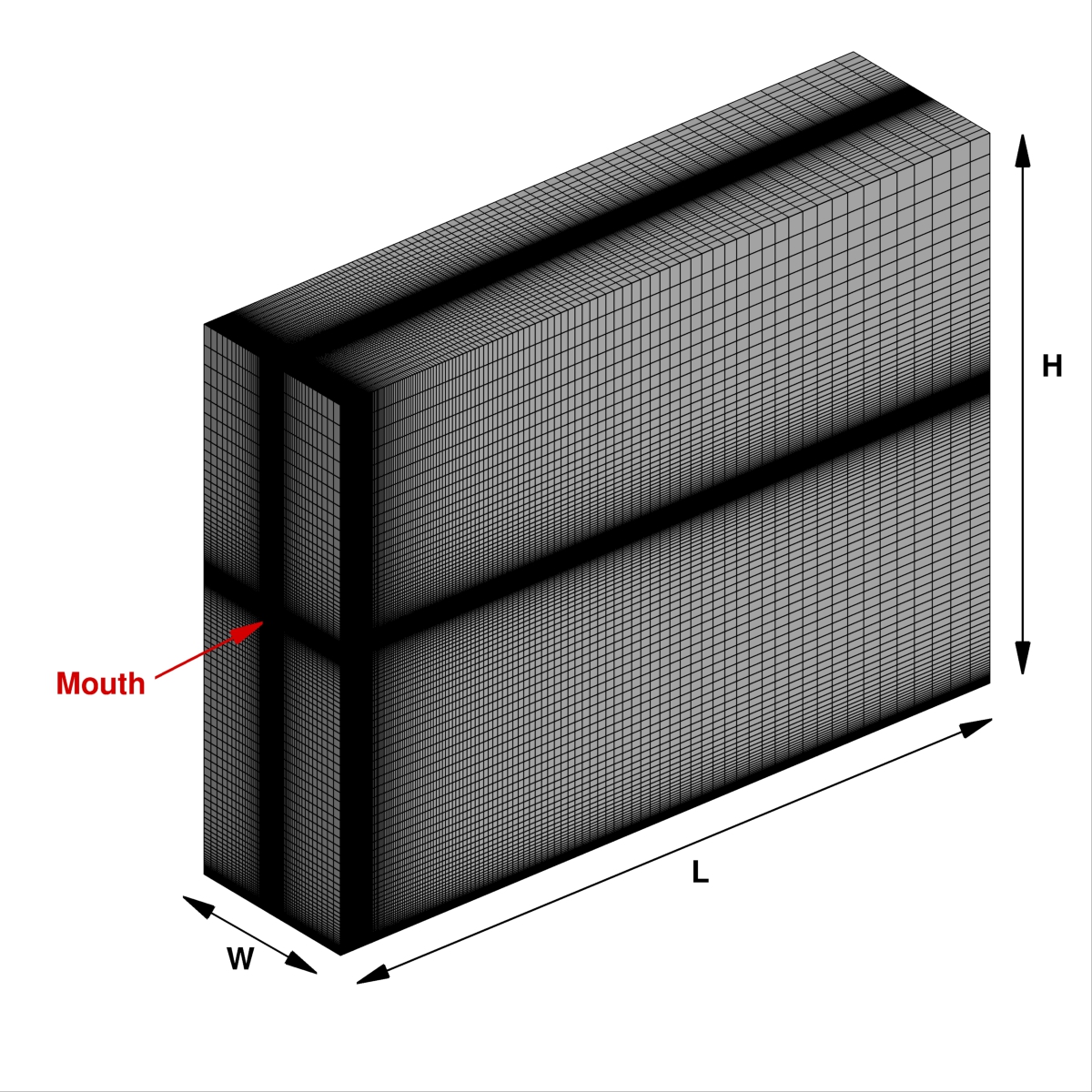
In the present work, a 3D computational domain was considered as shown in Fig. 1.
It consists of an air volume starting from the mouth–print of a standing coughing person.
A length , a width and a height were adopted, in accordance with Dbouk and Drikakis Dbouk and Drikakis 2020a.
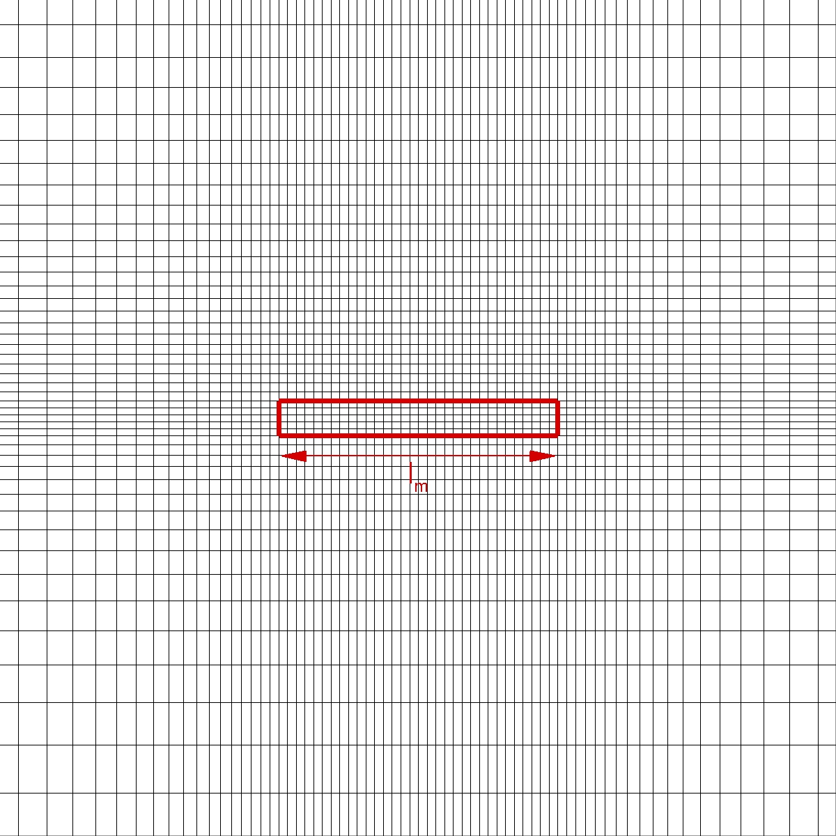
The mouth print is approximated as rectangular, having a length of
and a total area .
The reference frame origin, , is fixed in the same plane where
the mouth print is placed, see Fig. 1 and Fig. 2.
In particular, is in the middle of the previous face in correspondence with the intersection
of the domain bottom side.
–axis is aligned with bio–aerosol propagation direction; –axis represents transverse direction,
while –axis is the vertical direction.
The mouth–print centre, , was placed in the same position selected by Dbouk and Drikakis Dbouk and Drikakis 2020a:
.
Fully–structured meshes were built in order to discretise the domain.
A suite of three different grids named , and was generated
using, for all the cases, cells for mouth discretization.
Besides, mesh elements size grading was applied so as to achieve
a proper discretisation in the droplets’ emission and transport areas (Fig. 2).
The height of the first cell next to the ground, , was set at .
Other grids details are collected in Tab. 1.
| Grid | L points | W points | H points | Total |
|---|---|---|---|---|
| S1 | 170 | 112 | 150 | |
| S2 | 221 | 136 | 194 | |
| S3 | 270 | 158 | 231 |
III.2 Initial and boundary conditions
A stepped velocity inlet at the mouth boundary, with injection of parcels,
was applied to mimic the human cough over .
Velocity inlet value was deduced on the base of measurements carried on by Scharfman et al.Scharfman, B. E. and Techet, A. H. and Bush, J. W.
M. and Bourouiba, L. 2016, and
it is equal to in the streamwise direction both for carrier fluid and injected parcels.
In the same boundary turbulence intensity, , is fixed at and the mixing length equal to .
Furthermore, the initial total mass of saliva droplets laden into the domain is
according to the experimental measurements performed by Xie et al.Xie et al. 2012 and CFD simulations of Dbouk and DrikakisDbouk and Drikakis 2020a.
Saliva is, in general, a complex fluid but, following Van Der Reijden et al.Van Der Reijden, W.A. and Veerman, E.C.I. and Nieuw
Amerongen, A.V. 1993,
it could be approximated as water.
For this reason, the impact of the UV–C field on the parcels’ temperature is neglected
since UV–C water absorptivity is extremely low.
The remaining part of the – plane at is such that all the variables have
a null gradient through it.
The bottom side of the domain, i.e. the ground, is modelled as a standard
wall. Symmetry condition is imposed on lateral boundaries: .
On the other hand, zero gradient condition is set for all variables at the domain top with the exception
of the pressure. In this case, the pressure is reduced of its hydrostatic level.
The – plane at is managed as a physical outflow.
However, the pressure is imposed to decrease linearly, starting from atmospheric pressure
level at .
The initial temperature of the carrier fluid is with relative humidity
fixed at . The ground is at , while the air and droplets
ejected by human mouth are at .
The initial mass fraction composition of the Eulerian phase is: dry–air
and water–vapor as in Dbouk and Drikakis Dbouk and Drikakis 2020a.
The hypothesis of injection of saturated moist–air from the mouth is also taken into
account in the present work.
The estimated maximum Weber number is smaller than the critical oneSula, C. and Grosshans, H. and Papalexandris, M.
V. 2020, this
is the reason why any secondary breakup model is introduced in the following computations.
It is very important to put in evidence that previous initial conditions
are not adopted for our full computations.
Indeed, they are used as initial conditions of a preliminary simulation aimed
to generate adequate initial fields the full runs.
In this simulation, the transient condition
for mouth print boundary is not employed and treated like the remaining
part of the plane.
The preliminary simulations stage is considered
completed when a physical time of is reached.
It is worth emphasising that, after this precursor,
turbulent variables are initialised, and the hydrostatic pressure field,
not available in the previously described situation associated to an imposed uniform field, is obtained.
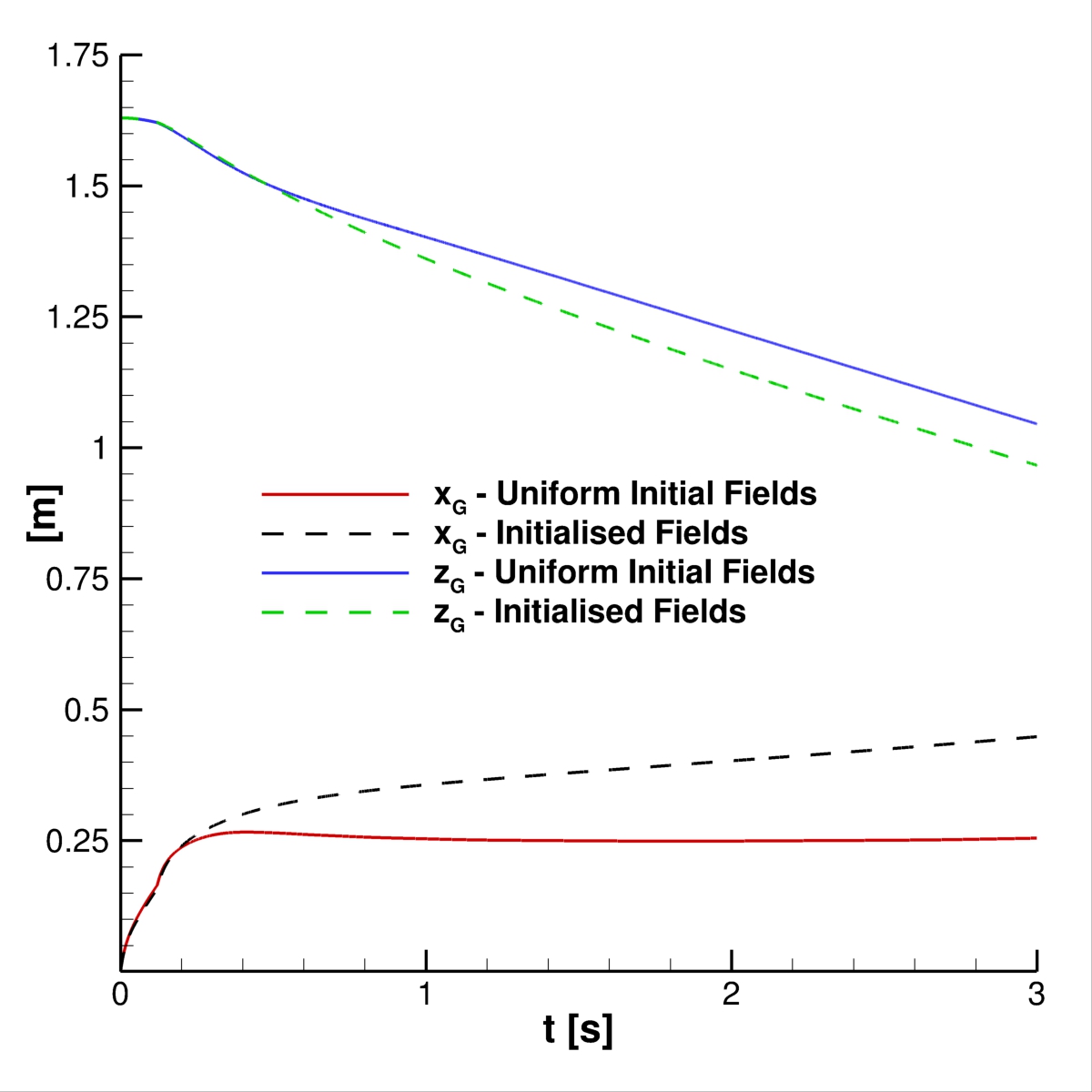
Cloud evolution is also strongly influenced as represented in Fig. 3.
Indeed, the cloud centre of mass position (defined in the next Section) in time completely
changes when initialised fields are employed.
IV Results
The present section shows the obtained numerical results referred to the bio–aerosol produced during coughing as cloud. Several cloud characteristics will be calculated and considered in order to investigate its diffusion and interaction with artificial UV–C light, i.e.
(i) cloud centre of mass; (ii) streamwise liquid penetration length; (iii) fraction of particles present in a reference volume; (iv) active fraction in a reference volume.The cloud centre of mass is computed as follows:
| (19) |
in eq. 19 is the overall number of parcels laden in the domain
in a given time–instant.
In the following lines is considered as the centre of mass components.
Streamwise liquid penetration length, , is defined as the maximum distance travelled along –axis
by a parcel conserving at least of its initial mass.
It is interesting to put in evidence that for this parameter, publicly available OpenFOAM functions are not used.
Thus, an inline function leaning on the parcel mass stored at the domain immission is developed.
Two different indexes for describing the saliva droplets’ population/activation are introduced.
The first index is the ratio between the number of particles present in a reference volume, , and the total
number of particles in the overall domain, , in a given time instant:
| (20) |
a second reference index is expressed in the following equation:
| (21) |
is the ratio of active particles in and the number of particles hosted
in . The aim of index is to provide a quantitative analysis
of the impact of UV–C related biological inactivation.
It is essential to remark that the data presented in this paper are focused on parallelpipedal reference volumes having the following features:
| (22) |
the parameter , appearing in eq. 22, spans the following values: , , , which
are selected in order to investigate a proper safety distance to be held in context of SARS–CoV–2 transmission
containment.
The transverse direction range is considered in order to completely cover the domain.
Lastly, axis interval is defined for acting on a sufficiently wide range of possible virus receivers’ heights.
All the computations were performed on the HPC–system CRESCO6 hosted by ENEA at Portici (Italy).
CRESCO6 comprises 434 nodes with two Intel Xeon Platinum 8160 24–core processors of the Skylake (SKL) generation operating at 2.1 GHz for each node.
There are 192 GB of RAM available in standard nodes.
The codes were built using Intel compilers and the MPI library version developed by Intel.
IV.1 Grid convergence study
A grid convergence study was carried out. Streamwise velocity profiles for the continuous phase were collected in order to evaluate the time evolution of the cough. In Fig. 4 and Fig. 5 the streamwise velocity, , behaviour in the mouth–print proximity is showed: and results are in good agreement both during the ejection phase and immediately after it has occurred. grid, instead, produces unphysical fluctuations in the entertainment zone. This is also true when the primary flux evolves into the domain (Fig. 6 -7).


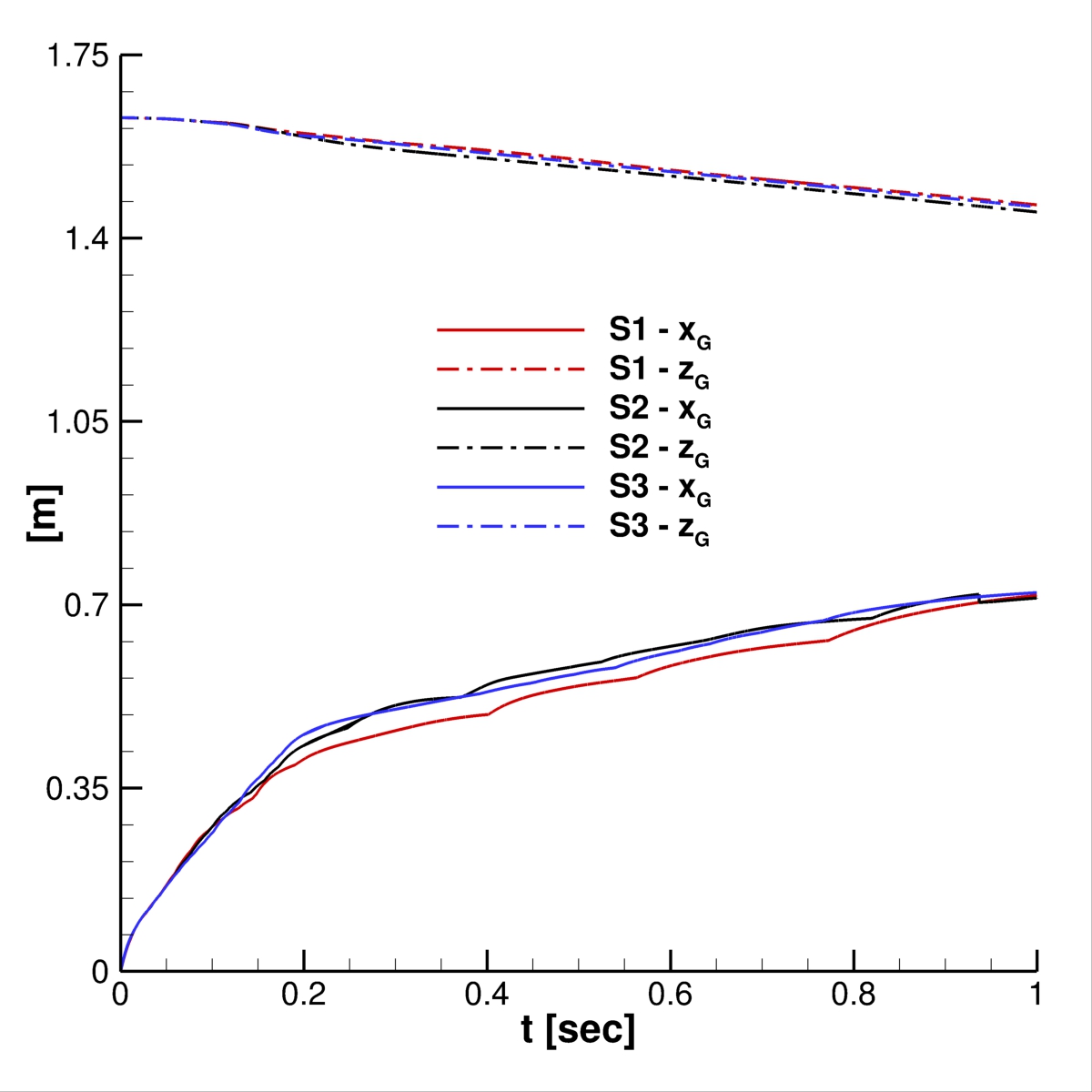
For what concerns the cloud development, its centre of mass position and time evolution were monitored.
Examining Fig. 8 is easy to see that and grids provide very similar behaviour. , instead,
underestimates , with a major impact on .
This is confirmed once again from the comparison in Fig. 9.
For this, was chosen as the best compromise between solution accuracy and computational load
for all the following simulations.
It is important to point out that, for the entire grid convergence study,
was adopted for computational efficiency reasons.

IV.2 Courant number effect
In the context of the dynamic adjustable time stepping technique adopted in this work, the evaluation of the correct is crucial. Five different maximum Courant numbers: were evaluated and their influence on the cloud properties was analysed. Fig. 10 put in evidence that, for , shows the same trajectory. In fact as well as time evolution are almost indistinguishable for the first three cases. A slightly different trend was found in the streamwise liquid penetration length (Fig. 11). In this case, , provided by assuming , does not perfectly replicates the behaviour given using lower ones. However, considering that the behaviour is slightly affected and the overall good results, is chosen for the investigations, even for ensure acceptable computing times.


IV.3 Particles per parcel effect
In the above discussed analyses a mean number of particle per parcel
was considered for the sake of efficiency in the Eulerian–Lagrangian framework coupling.
The intent is to complete the simulation parameters setting by means of the evaluation of
effect on the droplets’ cloud development. It is obvious that for each
particle is independent in its interaction with the carrier fluid and, consequently, the cloud parameters are not affected
by approximations due to the PSI–Cell method parcels based implementation.
Moreover, as noticeable in Fig. 12, using , the diameters of the particles
ejected during coughing, better fit the analytic Rosin–Rammler probability density function (PDF) distribution.
Finally, is adopted for the purpose of achieve the cloud proper modelling in terms of its
dynamical behaviour and PDF diameters size.

IV.4 Bio–aerosol transport and interaction with UV–C light
In this subsection, all relevant features, concerning SARS–CoV–2 transmission of saliva cloud derived from coughing, are examined. A representation of the computed cloud is showed in Fig 13–14.
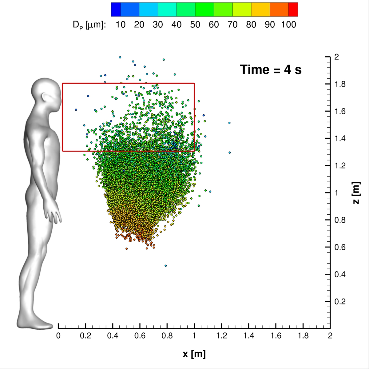

Note that the analyses will not be limited to a single cough ejection but also to multiple
ones.
Up to three cough cycles delayed by one over the otherDbouk and Drikakis 2020b are applied.
All the presented results are obtained from numerical simulations based on grid and
as showed in Secs. IV.1–IV.2. The simulated physical time,
excluding the precursor configuration, is (depending on breathing) due to the fact the
run is stopped when no parcels are still in the domain.
The total computation time of single case is about hours run in parallel using CPU–cores
on CRESCO6.
Fig. 15 depicts fraction of particles present in the four reference volumes
defined at the beginning of this section.
It is really interesting to note that curves are very close for .
So, regarding the possibility to receive infected particles when the external wind is not present,
distances ranging from to are equivalent.
A similar condition is highlighted in case of multiple cough ejections. Fig. 16
shows that similar droplets’ contamination is produced for and
for different coughing; results are not included in the plot
to avoid the unreadability of the chart.


In Fig. 17 streamwise liquid penetration length, , is depicted.
In the case of a single saliva droplets’ ejection is found;
differently, when the injections’ number increases rises to around .
It is also interesting to note that, after the first cough, the curve slope grows significantly and
the largest emitted particles travel not more than .

The centre of mass trajectory on the – plane is showed in Fig. 18.
The number of cough ejections does not affect largely evolution except for
its last portion.
For , the curve underlines a clear trend change.
Actually, in the proximity of this critical point the trajectory changes from
to almost linear one up to .
This is due to the cancellation of the inertial term.
In the last part of the curve, the evaporation and parcels’ interaction with the bottom wall lead to a complex
behaviour. The centre of mass trajectory suggests that several particles are located at distance over
from the emitter. Nevertheless, a very limited number is situated within the range .

The biological inactivation produced by UV–C light is analysed considering all the saliva
droplets introduced in the domain as fully active.
A commercial cylindrical lamp (having a radius of and length of ) is
used a UV–C source. It is positioned at the domain top and
different lamp layout were investigated. In the first case, the streamwise orientation was fixed
and the closer lamp edge to the mouth print is positioned in the point .
In the second configuration, the lamp is aligned to the crossflow direction and its centre is placed at .
Also two different power sizes were considered: and .
These values were selected in order to give a limited UV–C dose to a possible cough emitter in
accordance with Ultraviolet Radiation Guide published by Navy Environmental Health Center (USA)Navy Environmental Health
Center–USA 1992.
Looking at Tab. 2 is possible to observe the average and maximum UV–C dose (received in ) related
to mannequin placed at domain inlet region.
Table entries, connected to the average values, are deduced from a numerical integration of UV–C field irradiating the
space discretisated mannequin (only in its anterior portion) represented in Fig. 19.
| Case | Avg. dose | Max. dose |
|---|---|---|
| Streamwise - 55W | ||
| Crossflow - 55W | ||
| Crossflow - 25W |

The effect of UV–C lamp and orientation is clearly underlined in Fig. 20. The behaviour vis–à–vis time is evident for the reported cases. Anyway, the impact of the lamp orientation is barely noticeable; the lower power level lamp produces, according to the authors’ opinion, a modest biological inactivation of parcels. Thus, hereinafter the reference configuration uses a crossflow lamp.

The UV–C radiation inactivation capabilities are shown in Figs. 21–23. Only volume is studied since it is almost equivalent to and as regards the droplets’ presence. It is very important to stress that permanence time of droplets has scale for the different coughing. This condition can be also noted observing Fig. 14. Furthermore, UV–C light has a very good impact on the reduction of active particles. Indeed, index rapidly decreases in time reducing the contamination risk. In this context, it is interesting to note that after the number of parcels in is low and they are mainly located in its bottom side where UV–C field intensity suddenly decays, see Fig. 13. Therefore, the overall effect of this technique can be considered very promising.


V Conclusions
This paper addresses the development and application of an Eulerian–Lagrangian
model for saliva droplets’ cloud deriving from coughing.
Particular emphasis has been devoted to SARS–CoV–2 biological inactivation
produced by UV–C radiation at . Therefore, a new approach to
to model the UV–C inactivation effect was introduced.
A preliminary work was dedicated to the correct evaluation of grid points spacing
as well as and parcels’ injection features. Successively,
several relevant configurations have been analysed in absence of an external wind.
Moreover, two indexes were introduced
in order to provide quantitative informations about the contamination risk.
Firstable we noted that only a few particles get to distances grater than ,
in the vertical range , after different breathing conditions.
Hence, it may be confirmed that social distances greater than do not reduce
notably the possibility of receiving infected particles in not windy conditions.
Furthermore, it was also showed that UV–C radiation is a promising technique to perform a real–time
disinfection of a cloud resulting by coughing.
Indeed, the number of active particles can be significantly reduced during the saliva droplets’
cloud evolution without giving a critical UV–C dose to the emitter.
Acknowledgements.
The authors want to acknowledge Associazione Nazionale Big Data that awarded this research work within COVID19–Fast access to HPC supercomputing facilities programme. We acknowledge ENEA for awarding us access to CRESCO6 based at Portici.References
- Siegel et al. (2007) J. Siegel, E. Rhinehart, M. Jackson, and L. Chiarello, “Guideline for Isolation Precautions: Preventing Transmission of Infectious Agents in Healthcare Settings,” (2007), the Healthcare Infection Control Practices Advisory Committee, Atlanta, GA: U.S. Department of Health and Human Services.
- Mittal, Ni, and Seo (2020) R. Mittal, R. Ni, and J.-H. Seo, “The flow physics of COVID-19,” Journal of Fluid Mechanics 894 (2020), 10.1017/jfm.2020.330.
- Ai and A.K. (2018) Z. Ai and M. A.K., “Airborne spread of expiratory droplet nuclei between the occupants of indoor environments: A review,” Indoor 28, 500–524 (2018).
- Licina et al. (2014) D. Licina, J. Pantelic, A. Melikov, C. Sekhar, and K. Tham, “Experimental investigation of the human convective boundary layer in a quiescent indoor environment,” Building and Environment 75, 79 – 91 (2014).
- Nielsen (2015) P. Nielsen, “Fifty years of CFD for room air distribution,” Building and Environment 91, 78 – 90 (2015), fifty Year Anniversary for Building and Environment.
- Vuorinen et al. (2020) V. Vuorinen, M. Aarnio, M. Alava, M. Alopaeus, N. Atanasova, M. Auvinen, N. Balasubramanian, B. H., P. Erasto, R. Grande, N. Hayward, A. Hellsten, S. Hostikka, J. Hokkanen, O. Kaario, A. Karvinen, I. Kivisto, M. Korhonen, R. Kosonen, J. Kuusela, S. Lestinen, E. Laurila, H. Nieminen, P. Peltonen, J. Pokki, A. Puisto, P. Raback, H. Salmenjoki, T. Sironen, and M. Osterberg, “Modelling aerosol transport and virus exposure with numerical simulations in relation to SARS-CoV-2 transmission by inhalation indoors,” Safety Science 130, 104866 (2020).
- Pendar and Pascoa (2020) M. Pendar and J. Pascoa, “Numerical modeling of the distribution of virus carrying saliva droplets during sneeze and cough,” Physics of Fluids 32, 083305 (2020).
- Dbouk and Drikakis (2020a) T. Dbouk and D. Drikakis, “On coughing and airborne droplet transmission to humans,” Physics of Fluids 32 (2020a), 10.1063/5.0011960.
- Dbouk and Drikakis (2020b) T. Dbouk and D. Drikakis, “On respiratory droplets and face masks,” Physics of Fluids 32, 063303 (2020b).
- Dbouk and Drikakis (2020c) T. Dbouk and D. Drikakis, “Weather impact on airborne coronavirus survival,” Physics of Fluids 32, 093312 (2020c).
- Busco et al. (2020) G. Busco, S. Yang, J. Seo, and Y. A. Hassan, “Sneezing and asymptomatic virus transmission,” Physics of Fluids 32, 073309 (2020).
- Abuhegazy, M. and Talaat, K. and Anderoglu, O. and Poroseva, S. V. (2020) Abuhegazy, M. and Talaat, K. and Anderoglu, O. and Poroseva, S. V. , “Numerical investigation of aerosol transport in a classroom with relevance to COVID–19,” Physics of Fluids 32, 103311 (2020).
- Li,H. and Leong, F.Y. and Xu, G. and Ge, Z. and Kang,C.W. and Lim, K.H. (2020) Li,H. and Leong, F.Y. and Xu, G. and Ge, Z. and Kang,C.W. and Lim, K.H. , “Dispersion of evaporating cough droplets in tropical outdoor environment,” Physics of Fluids 32, 113301 (2020).
- Weller et al. (1998) H. Weller, G. Tabor, H. Jasak, and C. Fureby, “A tensorial approach to computational continuum mechanics using object–oriented techniques,” Computational Physics 12, 620–631 (1998).
- Buchan, Yang, and Atkinson (2020) A. Buchan, L. Yang, and K. D. Atkinson, “Predicting airborne coronavirus inactivation by far-UVC in populated rooms using a high-fidelity coupled radiation-CFD model,” Scientific Reports 10 (2020).
- Menter (1994) F. Menter, “Two-Equation Eddy Viscosity Turbulence Models for Engineering Applications,” AIAA Journal 32, 1598 – 1695 (1994).
- Crowe, Sharma, and Stock (1977) C. T. Crowe, M. P. Sharma, and D. E. Stock, “The Particle-Source-In Cell (PSI-CELL) Model for Gas-Droplet Flows,” Journal of Fluids Engineering 99, 325–332 (1977).
- Putnam (1961) A. Putnam, “Integratable form of droplet drag coefficient,” ARS J. 31, 1467 – 1468 (1961).
- Longest, P.W. and Jinxiang Xi, J. (2007) Longest, P.W. and Jinxiang Xi, J. , “Effectiveness of Direct Lagrangian Tracking Models for Simulating Nanoparticle Deposition in the Upper Airways,” Aerosol Science and Technology 41, 380–397 (2007).
- Zhao, B. and Zhang, Y. and Li, X. and Yang, X. and Huang, D. (2004) Zhao, B. and Zhang, Y. and Li, X. and Yang, X. and Huang, D., “Comparison of indoor aerosol particle concentration and deposition in different ventilated rooms by numerical method,” Building and Environment 39, 1 – 8 (2004).
- Ranz and Marshall (1952) W. E. Ranz and W. R. Marshall, “Evaporation from drops,” Chem. Eng. Prog. 48, 141 – 146 (1952).
- Mugele and Evans (1951) R. A. Mugele and H. D. Evans, “Droplet Size Distribution in Sprays,” Industrial & Engineering Chemistry 43, 1317–1324 (1951).
- Xie et al. (2012) X. Xie, Y. Li, H. Sun, and L. Liu, “Exhaled droplets due to talking and coughing,” J R Soc Interface (2012).
- Beggs, C.B. and Kerr, K.G. and Donnelly, J.K. and Sleigh, P.A. and Mara, D.D. and Cairns, G. (2000) Beggs, C.B. and Kerr, K.G. and Donnelly, J.K. and Sleigh, P.A. and Mara, D.D. and Cairns, G., “An engineering approach to the control of Mycobacterium tuberculosis and other airborne pathogens: A UK hospital based pilot study,” Transactions of the Royal Society of Tropical Medicine and Hygiene 94, 141–146 (2000).
- C.J. Noakes and L.A. Fletcher and C.B. Beggs and P.A. Sleigh and K.G. Kerr (2004) C.J. Noakes and L.A. Fletcher and C.B. Beggs and P.A. Sleigh and K.G. Kerr, “Development of a numerical model to simulate the biological inactivation of airborne microorganisms in the presence of ultraviolet light,” Journal of Aerosol Science 35, 489 – 507 (2004).
- Kowalski, W.J. Walsh, T.J. and Petraitis, V. (2020) Kowalski, W.J. Walsh, T.J. and Petraitis, V., “2020 COVID-19 Coronavirus ultraviolet susceptibility,” (2020).
- Modest (2014) M. Modest, Radiative Heat Transfer (Elsevier, New York, 2014).
- Kowalski et al. (2000) W. J. Kowalski, W. P. Bahnfleth, D. L. Witham, B. F. Severin, and T. S. Whittam, “Mathematical Modeling of Ultraviolet Germicidal Irradiation for Air Disinfection,” Quantitative Microbiology 2, 249–270 (2000).
- Issa (1986) R. Issa, “Solution of the implicitly discretised fluid flow equations by operator-splitting,” Journal of Computational Physics 62, 40–65 (1986).
- Scharfman, B. E. and Techet, A. H. and Bush, J. W. M. and Bourouiba, L. (2016) Scharfman, B. E. and Techet, A. H. and Bush, J. W. M. and Bourouiba, L., “Visualization of sneeze ejecta: steps of fluid fragmentation leading to respiratory droplets,” Experiments in Fluids 57, 24 (2016).
- Van Der Reijden, W.A. and Veerman, E.C.I. and Nieuw Amerongen, A.V. (1993) Van Der Reijden, W.A. and Veerman, E.C.I. and Nieuw Amerongen, A.V., “Shear rate dependent viscoelastic behavior of human glandular salivas,” Biorheology 30, 141–152 (1993).
- Sula, C. and Grosshans, H. and Papalexandris, M. V. (2020) Sula, C. and Grosshans, H. and Papalexandris, M. V., “Assessment of Droplet Breakup Models for Spray Flow Simulations,” Flow, Turbulence and Combustion 105, 889–914 (2020).
- Navy Environmental Health Center–USA (1992) Navy Environmental Health Center–USA, “Ultraviolet Radiation Guide,” (1992).