Selection Rule for Topological Amplifiers in Bogoliubov-de Gennes Systems
Abstract
Dynamical instability is an inherent feature of bosonic systems described by the Bogoliubov-de Gennes (BdG) Hamiltonian. Since it causes the BdG system to collapse, it is generally thought that it should be avoided. Recently, there has been much effort to harness this instability for the benefit of creating a topological amplifier with stable bulk bands but unstable edge modes which can be populated at an exponentially fast rate. We present a theorem for determining the stability of states with energies sufficiently away from zero, in terms of an unconventional commutator between the number conserving part and number nonconserving part of the BdG Hamiltonian. We apply the theorem to a generalization of a model from Galilo et al. [Phys. Rev. Lett, 115, 245302(2015)] for creating a topological amplifier in an interacting spin-1 atom system in a honeycomb lattice through a quench process. We use this model to illustrate how the vanishing of the unconventional commutator selects the symmetries for a system so that its bulk states are stable against (weak) pairing interactions. We find that as long as time reversal symmetry is preserved, our system can act like a topological amplifier, even in the presence of an onsite staggered potential which breaks the inversion symmetry.
pacs
Valid PACS appear hereI Introduction
The hallmark of topological matter is the presence of gapless edge modes that support the flow of currents along its boundaries in a manner immune to impurity scattering Hasan and Kane 2010; Qi and Zhang 2011. This property, which is as novel and fascinating as current flow without resistance in superconductivity Bardeen et al. 1957, follows from the nontrivial topology of Bloch band structures. As the Bloch band is a universal feature of any periodic systems, topological phenomena are ubiquitous, attracting intense interest across broad areas of research, including ultracold atoms Atala et al. 2013; Aidelsburger et al. 2013; Miyake et al. 2013; Jotzu et al. 2014; Stuhl et al. 2015, photons Haldane and Raghu 2008; Wang et al. 2009; Hafezi et al. 2011; Fang et al. 2012, phonons (and mechanical metamaterials) Kane and Lubensky 2013; Prodan and Prodan 2009; Fleury et al. 2014; Yang et al. 2015; Peano et al. 2015; He et al. 2016, and magnons Shindou et al. 2013a; Shindou et al. 2013b (see recent review articles Cooper et al. 2019; Ozawa et al. 2019; Zhang et al. 2018; Kondo et al. 2020 and references therein). This ubiquity also means that systems need no longer be closed, fermionic, Hermitian, and in thermal equilibrium in order to exhibit topological phases. Indeed, significant effort in recent years has been devoted to investigating open systems described by non-Hermitian Hamiltonians Esaki et al. 2011; Liang and Huang 2013; Lee 2016; Leykam and Chong 2016; Xiong 2018; Shen et al. 2018; Yao and Wang 2018 (see Gong et al. 2018; Kawabata et al. 2019; Zhou and Lee 2019; Ghatak and Das 2019; Ashida et al. 2020 and references therein).
In this paper, we consider quadratic bosonic systems Barnett 2013; Shindou et al. 2013b; Galilo et al. 2015; Engelhardt and Brandes 2015; Engelhardt et al. 2016; Bardyn et al. 2016; Peano et al. 2016; Furukawa and Ueda 2015; Shindou et al. 2013b. A new possibility arises in systems with bosons: Unrestricted by the Pauli exclusion principle, bosonic systems may be made to operate as active topological matter (a topological “laser”) where population amplification occurs only in modes localized along edges. Schomerus Schomerus 2013 sought to achieve this novel phase in a photonic crystal realization Poli et al. 2015 of the Su-Schrieffer-Heeger model Su et al. 1979, which is a non-Hermitian system with gain and loss. We focus on an alternative possibility Barnett 2013; Galilo et al. 2015; Engelhardt et al. 2016; Peano et al. 2016 which seeks to achieve the same goal in systems described by a quadratic bosonic Hamiltonian with pairing terms, which is the bosonic analog of the Bogoliubov-de Gennes (BdG) Hamiltonian for fermions.
The bosonic BdG system is Hermitian, but, unlike the fermionic BdG model, the matrix to be diagonalized is non-Hermitian. Hence, the bosonic BdG model inherits a so-called dynamical instability, which occurs when any subset of eigenvalues become complex. Recent proposals for realizing a topological amplifier in light Peano et al. 2016 and in matter Barnett 2013; Galilo et al. 2015; Engelhardt et al. 2016 make use of this dynamical instability.
This approach is not uncommon, as many exciting phenomena in physics are built on instabilities. For example, the production of highly coherent light in a laser follows from an instability associated with population inversion between upper and lower energy levels Sargent III et al. 1974 and the simultaneous amplification of signal and idler modes in light Milburn and Walls 1981; Slusher et al. 1985 and in matter Leslie et al. 2009; Campbell et al. 2006; Klempt et al. 2010 follows from a parametric instability Mandel and Wolf 1995 which occurs when the strength of the driving field exceeds a critical threshold.
A particular challenge with creating a topological amplifier lies in the dilemma that, on one hand, the topological amplifier must have an instability-free bulk (or, at least, a bulk far more stable than its edges) but, on the other hand, the dynamical instability in the bosonic BdG system tends to be impartial to edge and bulk states. An immediate question is how to control the instability so that it affects edge modes but not bulk modes. Answering this question is central to a successful implementation of topological amplifiers in BdG systems. The goal of the present work is to formulate a systematic approach to this question.
Our paper is organized as follows. In Sec. II, we consider a bosonic system described by a prototypical BdG Hamiltonian made up of number conserving (“normal”) and number nonconserving (“anomalous,” i.e., pairing) parts. It is well-known Wu and Niu 2001; Kawaguchi and Ohmi 2004; Nakamura et al. 2008 that complex eigenvalues and hence the dynamical instability in a bosonic BdG system can be traced to level crossings between particle and hole states in the absence of the pairing interaction. We thus focus on a pair of degenerate particle and hole states and investigate how the pairing interaction, which is treated as a perturbation, lifts the degeneracy. We combine first-order degenerate perturbation theory with the bi-orthonormality condition to establish a theorem for determining the stability of a state with energy sufficiently far from zero in a BdG system. Recognizing that the heart of the matter is level crossings between particle and hole states, we express this theorem in terms of an unconventional commutator between number conserving and number nonconserving parts of a BdG Hamiltonian [see Eq. (24)]. We show that when this “commutator” vanishes, the first-order splitting, which is purely imaginary, disappears and the two states remain stable and degenerate. We further show that when this “commutator” vanishes, the energy corrections remain real not only at second order in Sec. II but also to all higher orders in Appendix A. We thus identify the vanishing of the unconventional commutator (24) as a general and straightforward to use guiding principle for creating a topological amplifier in BdG systems.
In Appendix B, we describe a generalization of a model from Galilio et al. Galilo et al. 2015 for creating a topological amplifier in an interacting spin-1 atom system in a honeycomb lattice through a quench process. In Sec. III, we apply our theorem to this generalized model which is neither time reversal nor inversion symmetric and we use it to demonstrate how the principle we developed in Sec.II selects the symmetries that a BdG system must possess so that it may behave like a topological amplifier. We find that as long as time reversal symmetry is preserved, our system can act like a topological amplifier, even in the presence of an onsite staggered potential which breaks the inversion symmetry. We conclude in Sec. IV.
II A stability theorem for bosonic BdG systems
A topological amplifier in the context of the present work must have stable bulk states and unstable edge states. Then, a first step towards engineering such an amplifier is a good understanding of how a state in a BdG system can become unstable. In this section, we present a theorem which allows us to determine the stability of a state with energy sufficiently far from zero in a BdG system. Let such a (finite) system be described by the BdG Hamiltonian in Nambu space,
| (1) |
where stands for the crystal momentum (which may contain several components) within the first Brillouin zone. Equation (1) is not necessarily Hermitian, but since it is the BdG Hamiltonian for a Hermitian system, must be Hermitian, where the matrix is defined directly below Eq. (4). Consequently,
| (2) |
which are square matrices in an internal space and describe, respectively, number conserving and nonconserving (or pairing) processes. The BdG Hamiltonian (1) has two properties: so-called pseudo-Hermiticity,
| (3) |
and particle-hole symmetry
| (4) |
where and with the identity matrix in the internal space and and the Pauli and identity matrices in Nambu space, . No symmetry conditions have been imposed on our model; pseudo-Hermiciticy (3) and particle-hole symmetry (4) are intrinsic to the bosonic BdG Hamiltonian.
We briefly mention that pseudo-Hermiticity (3), while not a part of the Altland-Zirnbauer (AZ) symmetry classes Altland and Zirnbauer 1997, is a special case Lieu 2018 of so-called symmetry, one of the four fundamental Bernard-LeClair (BL) symmetry classes bernardAmdLeClair2002.207. The topological phases of bosonic BdG Hamiltonians are thus classified according to the BL-based 38-fold way for non-Hermitian systems Kawabata et al. 2019; Zhou and Lee 2019 — the culmination of recent efforts Esaki et al. 2011; Lieu 2018; Gong et al. 2018 for expanding the AZ-based 10-fold way from quadratic fermionic Hamiltonians Schnyder et al. 2008; Kitaev 2009; Ryu et al. 2010 to non-Hermitian Hamiltonians.
We assume the energy scale described by to be much larger than that described by , which allows us to split the total Hamiltonian according to , where
| (5) | ||||
| (6) |
are the unperturbed Hamiltonian and its perturbation, and
| (7) |
are projection and ladder operators in Nambu space.
A perturbative approach begins with the Schrödinger equation of the unperturbed BdG Hamiltonian,
| (8) |
where the unperturbed eigenstate , like any (stable) eigenstate of a BdG Hamiltonian, can be classified either as a particle state or as a hole state , depending on whether its norm with metric can be scaled to or Blaizot and Ripka 1986.
It thus obeys the so-called bi-orthonormality relation,
| (9) |
From now on, whenever no confusion is likely to arise, we ignore the argument to eigenenergies and eigenstates so as to reduce clutter in notations.
Let and be the eigenstates of the Hermitian matrix and with eigenvalues and , respectively,
| (10) |
where and obey the usual orthonormality relation,
| (11) |
within particle states and hole states, independently. In terms of and , the particle and hole states of Eq. (8) are given as
| (12) |
Nakamura et al. Nakamura et al. 2008, following earlier hints Wu and Niu 2001; Kawaguchi and Ohmi 2004, pointed out that the appearance of complex eigenvalues is always accompanied by a level crossing, i.e. a degeneracy between a hole and particle state when in the absence of pairing interactions. In the spirit of Nakamura et al. 2008, we focus on a particular particle and hole state of the unperturbed Hamiltonian,
| (13) |
which are degenerate with energy
| (14) |
and we hope to gain insight into how the pairing interaction lifts this degeneracy.
We first apply the standard perturbation ansatz,
| (15) |
to the Schrödinger equation
| (16) |
where and are the th order correction [in ] to the energy and corresponding eigenstate. In doing so, we arrive at a hierarchy of higher order equations,
| (17) | ||||
| (18) |
in addition to the zeroth order equation (8).
We then apply the degenerate perturbation ansatz in which is assumed to be the superposition of the degenerate states,
| (19) |
while is assumed to be the superposition of the particle and hole states,
| (20) |
where the primes are to stress that the degenerate states, and , are excluded from the first superposition over the particle states and the second superposition over the hole states, respectively.
We stress that since the unperturbed Hamiltonian (5) is Hermitian, all unperturbed eigenstates, upon which we make our perturbation expansion, are stable and form a complete Hilbert space. Further, in our derivation below, inner products are always between two unperturbed eigenstates. As a result, even though the total Hamiltonian (with pairing interactions) is pseudo-Hermitian, issues associated with a pseudo-Hermitian system such as zero modes and modes whose norms with metric vanish Blaizot and Ripka 1986, never arise throughout our derivation bellow.
Joining Eq. (17) with and (from the left), we arrive at the eigenvalue equation for ,
| (21) |
where use of the bi-orthonormality condition (9) has been made. The eigenvalue can be complex since the matrix in Eq. (21) can be non-Hermitian. Inserting Eq. (6) into Eq. (21), we simplify Eq. (21) into
| (22) |
from which we find
| (23) |
To write this in a more enlightening form, we introduce an unconventional commutator defined as
| (24) |
which is different from the conventional commutator unless is both real and even in . With the help of Eq. (10), we find that
| (25) |
which holds irrespective of whether and are the degenerate states. For the special case of the degenerate states, Eq. (25) becomes
| (26) |
which immediately leads to the following theorem.
Theorem 1
Let Eq. (1) be the BdG Hamiltonian for a bosonic system. Let a pair of particle and hole states be degenerate with energy in the absence of . Then, a weak lifts the degeneracy, splitting into a pair of complex conjugate energies, and , where is given by
| (27) |
which is valid to first order in , provided that
| (28) |
where is the unconventional commutator defined in Eq. (24) and and are the eigenstates defined in Eq. (10).
This theorem applies to a finite bosonic system described by a BdG Hamilonian in which the number nonconserving (pairing) part is much smaller in energy scale than the number conserving part and further the number conserving part supports degenerate particle and hole states. In the following, we shall refer to the states whose energies satisfy condition (28) as high- states.
Theorem 1 lin states that a pair of degenerate high- particle and hole states are unstable against if the transition between them is not -forbidden, where
| (29) |
is the effective coupling between the two degenerate states. Creating a stable BdG system amounts to developing selection rules for -forbidden transitions as far as first-order perturbation theory is concerned.
In particular, if “commutes” with , i.e., , all transitions between high- degenerate states are -forbidden. This raises the question of whether complex energies can arise from higher than first-order corrections, thereby causing the degenerate states to be unstable. To address this question, we have to extend the degenerate perturbation theory to second order because the degeneracy is not lifted at first order. We first join Eq. (18) with and , which leads to
| (30) |
We next employ Eq. (17) to express in terms of as
| (31) |
which involve inner products such as . It follows from Eq. (25) that when , the only chance for not to vanish is when and (which are the energies of states and ) are equal in magnitude but opposite in sign:
| (32) |
With this, Eq. (31) can be expressed as
| (33) |
Inserting this into Eq. (30), we find that the two equations in Eq. (30) decouple, leading immediately to two eigenstates: one with energy
| (34) |
and and and the other with energy
| (35) |
and and . We can remove the prime from each sum by virtue of Eq. (32). Finally, we apply, independently, the closure identities for and to cast and into the simpler forms,
| (36) |
which are real since they are the averages of two Hermitian operators, and . The Hermiticity of these two operators follows from in Eq. (2), a consequence of being inherently Hermitian. As we explain in Appendix A, this same property guarantees that the energy correction be real at any higher order, as long as .
It then follows that a sufficient condition for creating a stable high- state is that “commutes” with , i.e. the unconventional commutator (24) vanishes. This may be further understood by looking at the square of , which can be formulated in terms of as
| (37) |
where
| (38) |
is a Hermitian operator. From Eq. (37) we see that only when and “commute” is Hermitian. Thus, it is the condition [or equivalently ] that underlies the suggestion that systems with Hermitian may be made to operate in a manner free of bulk instabilities Galilo et al. 2015.
III Applications: A BdG extension of spinful Haldane model
In this section, we apply the theorem to a generalization of a model proposed by Galilo et al. Galilo et al. 2015 for creating a topological atom amplifier in spin-1 cold atoms in a honeycomb lattice through a quench process. In Appendix B, we give additional details for the (postquench) quadratic Hamiltonian describing quantum fluctuations about the initial state where all atoms are condensed to the spin-0 component. Just as in their model, the total Hamiltonian is divided into two independent sectors, one for the spin-0 component and the other for the spin- components. The spin- component is stable and not affected by the quench. The sector for spin- components is a BdG extension of a spinful Haldane model and evolves in time under the quench.
We thus focus on the spin- sector, a pseudo spin- system, on a lattice stripe geometry with open boundaries along and periodic (zigzag) boundaries along . The internal space is the tensor product , where is the unit cell space with the number of unit cells, is the spin- space, and is the sublattice space. We describe the system using the bosonic BdG Hamiltonian (1) with
| (39) |
where is a tridiagonal matrix (real and symmetric) with being the momentum vector along , is a diagonal matrix (real and -independent), and , and are the main-, sub- and super-diagonal identity matrices in . In Eq. (39),
| (40) |
are all real matrices in , where () and () are the Pauli (identity) matrices in and and . Here, is the nearest-neighbor hopping amplitude, is the next-nearest-neighbor hopping amplitude introduced by Haldane Haldane 1988, where alternates periodically in the manner of Kane and Mele Kane and Mele 2005, and measure, respectively, the nonstaggered and staggered onsite potential, is the filling factor for the condensed atoms, and is the two-body spin interaction strength Ho 1998; Ohmi and Machida 1998.

is neither time reversal nor inversion symmetric since we allow the phase and the staggered potential amplitude to be arbitrary where the time-reversal operator is defined as with being complex conjugation and the inversion symmetry operator is defined as (which is short for ). This is different than in Galilo et al. 2015, where and are fixed to and , respectively. Nor is -rotation invariant since although conserves , does not. Instead, it transforms under (which is short for ) in the manner of pseudo-Hermiticity,
| (41) |
due to spin and momentum conservation during a collision. Equation (41), together with the generic pseudo-Hermiticity in Eq. (3), implies the existence of a unitary symmetry, , where is the -component of the spin rotation generator represented on Nambu (particle-hole) space Altland and Zirnbauer 1997. Being diagonal, partitions into
| (42) |
where
| (43) |
are the Hamiltonians in the degenerate subspaces of in which has eigenvalue and , respectively. are matrices in that are constructed as follows. They take the form of in Eq. (39), where , and are matrices that are just as in Eq. (40), except is replaced with and is replaced with for and with for .
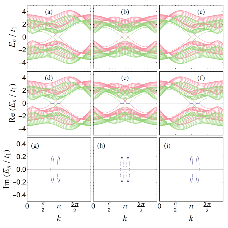
Without loss of generality, we limit our study to the sector. We focus on systems that have edge modes and band gaps near zero energy when (as shown in the top row of Figs. 1 and 2), so that the first-order perturbation theory may be applied to bulk states but not to edge modes near zero energy. We display the real (middle row) and imaginary (bottom row) eigenvalues of when in Fig. 1 where is fixed to 0 but is allowed to vary and in Fig. 2 where is fixed to but is allowed to vary.
To gain insight, we compute the “commutator” in Eq. (24), using Eqs. (39) and (40), to find
| (44) |
This result shows that only when (or ) and thus only when the system has time reversal symmetry, are bulk states stable in the presence of a paring term. This is evident in Fig. 1 where the bulk particle (red) and hole (green) energies that are degenerate when (top row) become complex when and takes values different from (left and right columns). Note that Eq. (44) is independent of the staggered potential . Thus, as long as it remains time-reversal-invariant, our system has a stable bulk even when it is no longer inversion-symmetric. Indeed, as Fig. 2 illustrates, the presence of does not affect bulk stability; all bulk spectra are real.
We now shed some light on why our system, like the one presented by Galilo et al. Galilo et al. 2015, is topological. As mentioned earlier, because our system conserves , partitions our system into two subsystems and our system inherits the topological properties of these two subsystems. Since the subsystems in our model are built upon the Haldane model, they inherit the Dirac points and point group symmetry, which are unaffected by the pairing interaction [the last line in Eq.(68)]. The point group symmetry guarantees that a gap closing and re-opening transition occurs only at Dirac points Bernevig and Hughes (see, for example, Furukawa and Ueda 2015). When the spectrum for an open system changes from one without edge modes inside the bulk gaps (not shown) to one with edge modes inside the bulk gaps (which is shown in Fig. 2), it signals that the corresponding periodic system makes a transition from a trivial gapped phase, via a gapless point at which the adiabatic condition breaks down, to a nontrivial gapped phase. This nontrivial gapped phase is a topological state with a nontrivial Chern number (i.e. it is a Chern insulator) since it is associated with a gap closing, which is a source of Berry curvature and hence nontrivial Chern number. In summary, our system is topological and is classified as two copies of Chern insulators. We leave as future work a detailed and quantitative study of the topological properties of our system, including how to identify its symmetry class within the framework of 38-fold way and how to determine its bulk topological variant (the Chern number) within the context of non-Hermitian physics Kawabata et al. 2019.
To study , where time reversal symmetry necessitates , we move to the basis Galilo et al. 2015, where is an eigenstate of ,
| (45) |
In this basis, we can take advantage and that pairing terms in Eq. (43) are proportional to the identity matrix , decomposing into a direct sum, , where
| (46) |
is a two-state Hamiltonian. We emphasize that this simplification holds regardless of the inversion symmetry. The eigenenergies in the sector are now easily found to be
| (47) |
As anticipated by Theorem 1, a Taylor series of does not contain the term linear in the small parameter, , and is real except when , where perturbation theory breaks down. Equation (47) also applies to edge modes. To a good approximation, we can estimate edge mode dispersions using Eq. (47) with given by
| (48) |
which are the edge mode dispersions of , the Hamiltonian of Haldane model (with ), for a lower half and upper half semi-infinite plane. Equation (48), which generalizes the one for in Galilo et al. 2015, indicates that constitutes another knob for selecting the momentum at which an edge mode is made to lase.
Note that we have checked for finite-size, e.g. is used to make Figs. 1 and 2 and is large enough that boundary states come in pairs localized to opposite ends. At the top edge (of the stripe lattice with open boundaries along ), the particle edge state moves to the right (the positive direction) while the hole edge state moves to the left. At the bottom edge, the particle edge state moves to the left while the hole edge state moves to the right.
Importantly, the staggered potential does not affect the bulk band stability in our model. We stress that the reason for this is that the staggered potential, in commutes with . If we included in a perturbation of the form which does not commute with the nearest-neighbor tunneling terms in , the “commutator” for the perturbed system with would become
| (49) |
and would thus not vanish even when the system is time-reversal-invariant. Even though and preserve both time and inversion symmetries, it is that affects bulk stability, and not , demonstrating that the “commutator” in Eq. (24) plays a fundamental role in the quest of topological amplifiers in BdG systems. Said another way, it is that selects the symmetries a system must possess so that its bulk states can be made stable against (weak) pairing interactions.
IV conclusion
In this work, we presented a theorem which quantifies how a weak pairing interaction lifts the degeneracy of particle and hole states with energy far from zero in a bosonic BdG system. We expressed the energy splitting, which is imaginary, in terms of the unconventional commutator in Eq. (24). We found that when , the property, , which is inherent of the BdG Hamiltonian guarantees the energy correction to be real at any higher order. We were thus led to treat the vanishing of this “commutator” as a practical criterion for testing and designing a topological amplifier in a BdG system. We also studied a generalization of the model from Galilo et al. Galilo et al. 2015, finding that as long as there is time reversal symmetry, the model can be made to act like a topological amplifier, independent of whether there is an inversion symmetry, i.e. independent of whether there exists an onsite staggered potential.
The theorem we developed is fairly general. Although we applied it only to a cold atom model in this work, we expect it to find applications in a broad array of systems across different disciplines Cooper et al. 2019; Ozawa et al. 2019; Zhang et al. 2018; Kondo et al. 2020; Gong et al. 2018.
Appendix A Higher than second-order energy corrections when and “commute”
In Sec. II, we focused on a particle and a hole state that are degenerate in the absence of the pairing interaction and found that when and “commute”, the pairing interaction, while does not contribute to the energy at first order, causes the energy to shift at second order from to and given by Eq. (36).
In this appendix, we pursue higher order corrections with the following perturbation equations,
| (50) | ||||
| (51) |
We begin with the third-order correction which depends not only on the zeroth- and first-order states, which we obtained in the main text, but also on the second-order state, which we now determine from Eq. (18). From Eq. (18),
| (52) |
which becomes, after applying Eq. (33),
| (53) |
In lieu of the restrictions by Eq. (32), the only possible contribution to the sum in [] in Eq. (53) comes from the hole (particle) state in which []. This means that all [] vanish except the one associated with the degenerate particle (hole) state () where []. However, it is precisely and , which are associated with the degenerate states, that are excluded from Eq. (20) for the second-order correction. We conclude that
| (54) |
The next step depends on whether equals , that is, whether the second order solution is degenerate or nondegenerate. In the degenerate case, the methods presented in Sec. II can be generalized to higher than second order. For this reason, we do not present them here. We instead present the nondegenerate case. Though we do not show it, it can be shown that the final results for the degenerate and nondegenerate cases are the same.
Let us briefly summarize the results through second order when . At second order and when , the pairing interaction splits the degenerate states, and , with energy into two states. The first state has , and
| (55) |
where is given by Eq. (36) and
| (56) |
which follows from Eq. (33) with . The second sate has and
| (57) |
where is given by Eq. (36) and
| (58) |
which follows from Eq. (33) with .
Under our assumption that degeneracy is lifted at second order, corrections higher than second order are computed with nondegenerate perturbation theory. Without loss of generality, we focus on the branch. We find easily from Eq. (50), with the help of Eq. (55), that
| (59) |
where
| (60) |
with the last equality following from Eq. (32) and Eq. (56). From Eq. (51), we then have the fourth-order correction to the energy,
| (61) |
which, when use of Eq. (60) is made, can be written as
| (62) |
Compared to Eq. (34), we find that the second line is simply , and thus
| (63) |
Since and are both real, so too is .
Generalizing to higher orders is straightforward. Upon doing so, one finds that all odd higher-order energy corrections vanish while all higher-order even ones can be expressed in terms of and and are therefore real. We note that this same conclusion is found if we had instead assumed that the second order corrections are degenerate.
We end this appendix by stressing that a bosonic BdG Hamiltonian has an intrinsic property that is Hermitian, which ensures . And when , it is that guarantees the energy correction to be real at any order in perturbation theory.
Appendix B Hamiltonian for a BdG extension of a spinful Haldane model
In the main text, we study a generalization of a model proposed by Galilo et al. Galilo et al. 2015. In this Appendix, we provide details of the Hamiltonian for this generalization. Motivated by the experimental realization of the Haldane model Haldane 1988 by the Esslinger group Jotzu et al. 2014 in ultracold atoms in honeycomb optical lattices, Galilo et al. Galilo et al. 2015 proposed a spin-1 extension of such a system where the spin-orbit coupling is proportional to the spin projection along , , where are the spin components of the spin-1 vector . The generalization we study has a Hamiltonian consisting of three parts. First, the hopping Hamiltonian
| (65) |
where is the field operator, is the annihilation operator of a boson with spin- component at site , is the nearest-neighbor hopping amplitude, and is the next-nearest-neighbor hopping amplitude introduced by Haldane Haldane 1988, where alternates between and periodically in the manner of Kane and Mele Kane and Mele 2005. Second, the onsite two-body interaction that preserves the spin rotation invariance Ho 1998; Ohmi and Machida 1998,
| (66) |
where and represent, respectively, the density and spin interaction strength. The onsite collision is the source of pairing interactions, which is an essential ingredient of a BdG system. Third, the onsite potential (with staggering)
| (67) |
which describes the quadratic Zeeman shifts for spinor condensates which can be generated by external magnetic fields Stamper-Kurn and Ueda 2013 or by microwave fields Gerbier et al. 2006 where is for sites on sublattice and for sites on sublattice .
As in Galilo et al. 2015, the onsite potential initially supports a polar condensate where all atoms are condensed to the spin mode and are assumed to be uniformly distributed in space. We then apply a quench process, which abruptly changes the onsite potential. Previously, spin-1 condensates were quenched to demonstrate intriguing nonequilibrium dynamics Leslie et al. 2009; Lamacraft 2007; Stamper-Kurn and Ueda 2013. We characterize this uniform polar condensate with a filling factor for condensed bosons and a chemical potential at which the energy per lattice site is minimized. We note that such a polar state is energetically favored as long as is set to a sufficiently large positive value.
Following the usual practice (see, for example, Kain and Ling 2014), we apply the Bogoliubov perturbation ansatz to the postquench Hamiltonian where the system parameters are fixed at their quenched values. When expanded up to second order in = , which are the field operators describing quantum fluctuations on top of the condensate, we find the postquench Hamiltonian to be block diagonal,
| (68) |
where
| (69) |
is the Hamiltonian in the pseudo spin- space , where and are the Pauli and identity matrices in spin space and
| (70) |
As can be seen, without pairing terms, in Eq. (69) represents the spinful (doubled) Haldane model. Thus, with pairing terms, it describes what we call a BdG extension of spinful Haldane model. Note that we have used a lowercase instead of capital to distinguish between spin- and spin- systems. In Eq. (68), (which we have not shown) is the Hamiltonian for the component which always has a stable spectrum (for weak ) and is not affected by the quench.

We focus exclusively on the spin- system in a honeycomb lattice. We assume a stripe geometry with open boundaries along and periodic (zigzag) boundaries along . We apply a partial Fourier transformation along ,
| (71) |
where () is the number of unit cells along (), is the momentum vector along , and is the -component of the position vector at site . Finally, with the help of the basis vectors defined in Fig. 3, we change the Hamiltonian (69) to
| (72) |
where is the Nambu spinor and is the bosonic BdG Hamiltonian given by Eq. (1) with the matrix defined directly below Eq. (4). Here, is the vector field and and in Eq. (1) are matrices given by Eq. (39) in the internal space which is now the tensor product between the -unit cell space, the spin space and the sublattice space defined in the main text. For convenience, we change to and to in the main text.
References
- Hasan and Kane (2010) M. Z. Hasan and C. L. Kane, Colloquium : Topological insulators, Rev. Mod. Phys. 82, 3045 (2010).
- Qi and Zhang (2011) X.-L. Qi and S.-C. Zhang, Topological insulators and superconductors, Rev. Mod. Phys. 83, 1057 (2011).
- Bardeen et al. (1957) J. Bardeen, L. N. Cooper, and J. R. Schrieffer, Theory of superconductivity, Phys. Rev. 108, 1175 (1957).
- Atala et al. (2013) M. Atala, M. Aidelsburger, J. T. Barreiro, D. Abanin, T. Kitagawa, E. Demler, and I. Bloch, Direct measurement of the zak phase in topological bloch bands, Nat. Phys. 9, 795 (2013).
- Aidelsburger et al. (2013) M. Aidelsburger, M. Atala, M. Lohse, J. T. Barreiro, B. Paredes, and I. Bloch, Realization of the hofstadter hamiltonian with ultracold atoms in optical lattices, Phys. Rev. Lett. 111, 185301 (2013).
- Miyake et al. (2013) H. Miyake, G. A. Siviloglou, C. J. Kennedy, W. C. Burton, and W. Ketterle, Realizing the harper hamiltonian with laser-assisted tunneling in optical lattices, Phys. Rev. Lett. 111, 185302 (2013).
- Jotzu et al. (2014) G. Jotzu, M. Messer, R. Desbuquois, M. Lebrat, T. Uehlinger, D. Greif, and T. Esslinger, Experimental realization of the topological haldane model with ultracold fermions, Nature 515, 237 (2014).
- Stuhl et al. (2015) B. K. Stuhl, H.-I. Lu, L. M. Aycock, D. Genkina, and I. B. Spielman, Visualizing edge states with an atomic bose gas in the quantum hall regime, Science 349, 1514 (2015).
- Haldane and Raghu (2008) F. D. M. Haldane and S. Raghu, Possible realization of directional optical waveguides in photonic crystals with broken time-reversal symmetry, Phys. Rev. Lett. 100, 013904 (2008).
- Wang et al. (2009) Z. Wang, Y. Chong, J. D. Joannopoulos, and M. Soljačić, Observation of unidirectional backscattering-immune topological electromagnetic states, Nature 461, 772 (2009).
- Hafezi et al. (2011) M. Hafezi, E. A. Demler, M. D. Lukin, and J. M. Taylor, Robust optical delay lines with topological protection, Nat. Phys. 7, 907 (2011).
- Fang et al. (2012) K. Fang, Z. Yu, and S. Fan, Realizing effective magnetic field for photons by controlling the phase of dynamic modulation, Nat. Photon 6, 792 (2012).
- Kane and Lubensky (2013) C. L. Kane and T. C. Lubensky, Topological boundary modes in isostatic lattices, Nat. Phys. 10, 39 (2013).
- Prodan and Prodan (2009) E. Prodan and C. Prodan, Topological phonon modes and their role in dynamic instability of microtubules, Phys. Rev. Lett. 103, 248101 (2009).
- Fleury et al. (2014) R. Fleury, D. L. Sounas, C. F. Sieck, M. R. Haberman, and A. Alù, Sound isolation and giant linear nonreciprocity in a compact acoustic circulator, Science 343, 516 (2014).
- Yang et al. (2015) Z. Yang, F. Gao, X. Shi, X. Lin, Z. Gao, Y. Chong, and B. Zhang, Topological acoustics, Phys. Rev. Lett. 114, 114301 (2015).
- Peano et al. (2015) V. Peano, C. Brendel, M. Schmidt, and F. Marquardt, Topological phases of sound and light, Phys. Rev. X 5, 031011 (2015).
- He et al. (2016) C. He, X. Ni, H. Ge, X.-C. Sun, Y.-B. Chen, M.-H. Lu, X.-P. Liu, and Y.-F. Chen, Acoustic topological insulator and robust one-way sound transport, Nat. Phys. 12, 1124 (2016).
- Shindou et al. (2013a) R. Shindou, J.-i. Ohe, R. Matsumoto, S. Murakami, and E. Saitoh, Chiral spin-wave edge modes in dipolar magnetic thin films, Phys. Rev. B 87, 174402 (2013a).
- Shindou et al. (2013b) R. Shindou, R. Matsumoto, S. Murakami, and J.-i. Ohe, Topological chiral magnonic edge mode in a magnonic crystal, Phys. Rev. B 87, 174427 (2013b).
- Cooper et al. (2019) N. R. Cooper, J. Dalibard, and I. B. Spielman, Topological bands for ultracold atoms, Rev. Mod. Phys. 91, 015005 (2019).
- Ozawa et al. (2019) T. Ozawa, H. M. Price, A. Amo, N. Goldman, M. Hafezi, L. Lu, M. C. Rechtsman, D. Schuster, J. Simon, O. Zilberberg, and I. Carusotto, Topological photonics, Rev. Mod. Phys. 91, 015006 (2019).
- Zhang et al. (2018) X. Zhang, M. Xiao, Y. Cheng, M.-H. Lu, and J. Christensen, Topological sound, Commun. Phys 1, 97 (2018).
- Kondo et al. (2020) H. Kondo, Y. Akagi, and H. Katsura, Non-hermiticity and topological invariants of magnon bogoliubov–de gennes systems, Prog. Theor. Exp. Phys. 2020, 12A104 (2020).
- Esaki et al. (2011) K. Esaki, M. Sato, K. Hasebe, and M. Kohmoto, Edge states and topological phases in non-hermitian systems, Phys. Rev. B 84, 205128 (2011).
- Liang and Huang (2013) S.-D. Liang and G.-Y. Huang, Topological invariance and global berry phase in non-hermitian systems, Phys. Rev. A 87, 012118 (2013).
- Lee (2016) T. E. Lee, Anomalous edge state in a non-hermitian lattice, Phys. Rev. Lett. 116, 133903 (2016).
- Leykam and Chong (2016) D. Leykam and Y. D. Chong, Edge solitons in nonlinear-photonic topological insulators, Phys. Rev. Lett. 117, 143901 (2016).
- Xiong (2018) Y. Xiong, Why does bulk boundary correspondence fail in some non-hermitian topological models, J. Phys. Commun 2, 035043 (2018).
- Shen et al. (2018) H. Shen, B. Zhen, and L. Fu, Topological band theory for non-hermitian hamiltonians, Phys. Rev. Lett. 120, 146402 (2018).
- Yao and Wang (2018) S. Yao and Z. Wang, Edge states and topological invariants of non-hermitian systems, Phys. Rev. Lett. 121, 086803 (2018).
- Gong et al. (2018) Z. Gong, Y. Ashida, K. Kawabata, K. Takasan, S. Higashikawa, and M. Ueda, Topological phases of non-hermitian systems, Phys. Rev. X 8, 031079 (2018).
- Kawabata et al. (2019) K. Kawabata, K. Shiozaki, M. Ueda, and M. Sato, Symmetry and topology in non-hermitian physics, Phys. Rev. X 9, 041015 (2019).
- Zhou and Lee (2019) H. Zhou and J. Y. Lee, Periodic table for topological bands with non-hermitian symmetries, Phys. Rev. B 99, 235112 (2019).
- Ghatak and Das (2019) A. Ghatak and T. Das, New topological invariants in non-hermitian systems, Journal of Physics: Condensed Matter 31, 263001 (2019).
- Ashida et al. (2020) Y. Ashida, Z. Gong, and M. Ueda, Non-hermitian physics, Advances in Physics 69, 249 (2020).
- Barnett (2013) R. Barnett, Edge-state instabilities of bosons in a topological band, Phys. Rev. A 88, 063631 (2013).
- Galilo et al. (2015) B. Galilo, D. K. K. Lee, and R. Barnett, Selective population of edge states in a 2d topological band system, Phys. Rev. Lett. 115, 245302 (2015).
- Engelhardt and Brandes (2015) G. Engelhardt and T. Brandes, Topological bogoliubov excitations in inversion-symmetric systems of interacting bosons, Phys. Rev. A 91, 053621 (2015).
- Engelhardt et al. (2016) G. Engelhardt, M. Benito, G. Platero, and T. Brandes, Topological instabilities in ac-driven bosonic systems, Phys. Rev. Lett. 117, 045302 (2016).
- Bardyn et al. (2016) C.-E. Bardyn, T. Karzig, G. Refael, and T. C. H. Liew, Chiral bogoliubov excitations in nonlinear bosonic systems, Phys. Rev. B 93, 020502 (2016).
- Peano et al. (2016) V. Peano, M. Houde, F. Marquardt, and A. A. Clerk, Topological quantum fluctuations and traveling wave amplifiers, Phys. Rev. X 6, 041026 (2016).
- Furukawa and Ueda (2015) S. Furukawa and M. Ueda, Excitation band topology and edge matter waves in bose-einstein condensates in optical lattices, New Journal of Physics 17, 115014 (2015).
- Schomerus (2013) H. Schomerus, Topologically protected midgap states in complex photonic lattices, Opt. Lett. 38, 1912 (2013).
- Poli et al. (2015) C. Poli, M. Bellec, U. Kuhl, F. Mortessagne, and H. Schomerus, Selective enhancement of topologically induced interface states in a dielectric resonator chain, Nat. Commun. 6, 6710 (2015).
- Su et al. (1979) W. P. Su, J. R. Schrieffer, and A. J. Heeger, Solitons in polyacetylene, Phys. Rev. Lett. 42, 1698 (1979).
- Sargent III et al. (1974) M. Sargent III, M. O. Scully, and W. E. Lamb Jr., Laser physics, CRC Press, New York (1974).
- Milburn and Walls (1981) G. Milburn and D. F. Walls, Production of squeezed states in a degenerate parametric amplifier, Opt. Commun. 39, 401 (1981).
- Slusher et al. (1985) R. E. Slusher, L. W. Hollberg, B. Yurke, J. C. Mertz, and J. F. Valley, Observation of squeezed states generated by four-wave mixing in an optical cavity, Phys. Rev. Lett. 55, 2409 (1985).
- Leslie et al. (2009) S. R. Leslie, J. Guzman, M. Vengalattore, J. D. Sau, M. L. Cohen, and D. M. Stamper-Kurn, Amplification of fluctuations in a spinor bose-einstein condensate, Phys. Rev. A 79, 043631 (2009).
- Campbell et al. (2006) G. K. Campbell, J. Mun, M. Boyd, E. W. Streed, W. Ketterle, and D. E. Pritchard, Parametric amplification of scattered atom pairs, Phys. Rev. Lett. 96, 020406 (2006).
- Klempt et al. (2010) C. Klempt, O. Topic, G. Gebreyesus, M. Scherer, T. Henninger, P. Hyllus, W. Ertmer, L. Santos, and J. J. Arlt, Parametric amplification of vacuum fluctuations in a spinor condensate, Phys. Rev. Lett. 104, 195303 (2010).
- Mandel and Wolf (1995) L. Mandel and E. Wolf, Optical coherence and quantum optics, Cambridge University Press, New York (1995).
- Wu and Niu (2001) B. Wu and Q. Niu, Landau and dynamical instabilities of the superflow of bose-einstein condensates in optical lattices, Phys. Rev. A 64, 061603 (2001).
- Kawaguchi and Ohmi (2004) Y. Kawaguchi and T. Ohmi, Splitting instability of a multiply charged vortex in a bose-einstein condensate, Phys. Rev. A 70, 043610 (2004).
- Nakamura et al. (2008) Y. Nakamura, M. Mine, M. Okumura, and Y. Yamanaka, Condition for emergence of complex eigenvalues in the bogoliubov–de gennes equations, Phys. Rev. A 77, 043601 (2008).
- Altland and Zirnbauer (1997) A. Altland and M. R. Zirnbauer, Nonstandard symmetry classes in mesoscopic normal-superconducting hybrid structures, Phys. Rev. B 55, 1142 (1997).
- Lieu (2018) S. Lieu, Topological symmetry classes for non-hermitian models and connections to the bosonic bogoliubov–de gennes equation, Phys. Rev. B 98, 115135 (2018).
- (59) D. Bernard and A. LeClair, A classification of non-hermitian random matrices, in Statistical Field Theories, edited by A. Cappelli and G. Mussardo (Spring Netherland, Dordrecht, 2002), p. 207.
- Schnyder et al. (2008) A. P. Schnyder, S. Ryu, A. Furusaki, and A. W. W. Ludwig, Classification of topological insulators and superconductors in three spatial dimensions, Phys. Rev. B 78, 195125 (2008).
- Kitaev (2009) A. Kitaev, AIP Conference Proceedings 1134, 22 (2009).
- Ryu et al. (2010) S. Ryu, A. P. Schnyder, A. Furusaki, and A. W. W. Ludwig, Topological insulators and superconductors: tenfold way and dimensional hierarchy, New Journal of Physics 12, 065010 (2010).
- Blaizot and Ripka (1986) J.-P. Blaizot and G. Ripka, Quanum theory of finite systems, The MIT Press, Cambridge, MA (1986).
- (64) Although derived from a BdG Hamiltonian that depends on crystal momentum , this dependency is not essential. .
- Haldane (1988) F. D. M. Haldane, Model for a quantum hall effect without landau levels: Condensed-matter realization of the ”parity anomaly”, Phys. Rev. Lett. 61, 2015 (1988).
- Kane and Mele (2005) C. L. Kane and E. J. Mele, topological order and the quantum spin hall effect, Phys. Rev. Lett. 95, 146802 (2005).
- Ho (1998) T.-L. Ho, Spinor bose condensates in optical traps, Phys. Rev. Lett. 81, 742 (1998).
- Ohmi and Machida (1998) T. Ohmi and K. Machida, Bose-einstein condensation with internal degrees of freedom in alkali atom gases, Journal of the Physical Society of Japan 67, 1822 (1998).
- (69) B. A. Bernevig and T. L. Hughes, Topological Insulators and Topological Superconductors (Princeton University Press, Princeton, 2013) .
- Stamper-Kurn and Ueda (2013) D. M. Stamper-Kurn and M. Ueda, Spinor bose gases: Symmetries, magnetism, and quantum dynamics, Rev. Mod. Phys. 85, 1191 (2013).
- Gerbier et al. (2006) F. Gerbier, A. Widera, S. Fölling, O. Mandel, and I. Bloch, Resonant control of spin dynamics in ultracold quantum gases by microwave dressing, Phys. Rev. A 73, 041602 (2006).
- Lamacraft (2007) A. Lamacraft, Quantum quenches in a spinor condensate, Phys. Rev. Lett. 98, 160404 (2007).
- Kain and Ling (2014) B. Kain and H. Y. Ling, Nonequilibrium states of a quenched bose gas, Phys. Rev. A 90, 063626 (2014).