Bumblebee gravity with a Kerr-Sen-like solution and its Shadow

Various kinds of astronomical observations strongly confirm the existence of the black-hole in the Universe. The recent message of the detection of gravitational waves (GWs)GVW by the $LIGO$ and $VIRGO$ observatories, and the captured image of the black-hole shadow of a super-massive $M87^{*}$ black-hole by the Event Horizon Telescope EVENT; EVENT1 provides substantial evidence in support of the existence of black-hole. The perception of the fundamental nature of spacetime would also likely to be enriched with the information accessible from these recent astronomical observations. So physics of black-hole acquire renewed interest.

General relativity and the standard model of particle physics are two very successful field theoretical models that assist us to describe our Universe. The formulation of both these theories is based on the well celebrated Lorentz symmetry. However, the regime of applicability and the nature of service towards describing the Universe by these two theories are profoundly different. The general relativity describes the gravitational interaction and it is a classical field theory in the curved spacetime and there is no direct way to include the quantum effect. On the contrary, the standard model describes the other fundamental interactions and it is the quantum field theory in the flat spacetime that neglects all gravitational effects, but to study the physical system in the vicinity of the Plank scale $(10^{-19}GeV)$, the effect due to gravity cannot be ignored, since the gravitational interaction is strong enough in that energy scale. Therefore, the study of physics in the vicinity of the Planck scale necessarily entails the unification of general relativity and standard model particle physics. Unfortunately, it is not yet developed with its full wings because there is no straightforward way to quantize gravity. Moreover, Lorentz invariance is not tenable in the regime where spacetime is discrete in nature. So in the vicinity of the Planck scale, it would not be unreasonable to discard Lorentz invariance. On the other hand, Lorentz symmetry breaking in nature is considered as an interesting and useful idea because it arises as a possibility in the context of string theory STRING1; STRING2; STRING3; STRING4, noncommutative field theories NONCOM or loop quantum gravity theory LOOP1; LOOP2. As a consequence, nowadays Lorentz violation is considered as relevant as well as a beneficial tool to probe the foundations of modern physics. This fact suggests that signals associated with LV is a promising way to investigate quantum gravity at the Planck scale. The LV in the neutrino sector NEUTRINO, the standard model extension (SME) ESM, and the LV effect on the formation of atmospheric shower SHOAT are some important studies involving LV in this regard.

The effective theory that would capture of the Plank scale effect at least in a coarse-grained manner should encompass LV effect through some LV sector. The Standard Model Extension (SME) is an effective field theory which is worth mentioning that describes the general relativity and the standard model at low energies, that includes additional terms containing information about the LV occurring at the Planck scale ESM; ESM1; ESM2; ESM3. The electromagnetic sector of the SME has been extensively studied in the literature EMS1; EMS2; EMS3; EMS4; EMS5; EMS6; EMS7; EMS8; EMS9; EMS10; EMS11; EMS12; EMS13; EMS14; EMS15; EMS16; EMS17. The electro-weak sector of it is described in the articles EE1; EE2. Furthermore, some effects of LV in the gravitational sector have been studied in GVL1; GVL2; GVL3; GVL4; GVL5, specifically the case of the gravitational waves was analyzed in the article GVW1; GVW2.

For any theory of gravity, looking for a black-hole solution is a significantly important extension, since black-holes provide into the quantum gravity realm. In this respect, rotating black-hole solutions are the most relevant subjects for astrophysics KERR; KERRNU; ASEN. It is known that the LV effect can be instigated in the gravitational sector inviting the valuable service of bumblebee field. In DING, an attempt has been made to find out an exact Kerr-like solution through solving Einstein-bumblebee equations. In earlier work, Casana et al. found an exact Schwarzschild-like solution in this bumblebee gravity model and investigated its some classical tests RC. Then Rong-Jia Yang et al. study the accretion onto this black-hole RONG and find the LV parameter $\ell$ will slow down the mass accretion rate. Sequential development entails that the Kerr-sen-like solution from Einstein-bumblebee would also be of worth investigation. It would be useful when the black-hole contains both charge and angular momentum. We, therefore make an attempt to seek a Kerr-sen-like solution from the Einstein-bumblebee equations of motion.

The paper is organized as follows. Sect. II contains a review of the Einstein-Bumblebee theory. In Sect. III, we find out an exact Kerr-Sen-like black-hole solution from Einstein-Bumblebee theory with the evaluation of Hawking temperature. Sect. IV is devoted to the motion of photon and the sketching of black-hole shadow. How this shadow deforms with $\ell$ is also investigated. In Sect. V, the emission rate of radiation has been studied and how it varies with $\ell$ is also observed closely. Sect. VI contains a summary and discussion of the work.

Einstein-Bumblebee theory (or simply bumblebee model)is an effective field theory where a vector field receives vacuum expectation value (VEV)through spontaneous symmetry breaking. The action of which is given by

$\displaystyle\mathcal{S}=\int d^{4}x\sqrt{-g}\left[\frac{1}{16\pi G_{N}}\left(\mathcal{R}+\varrho B^{\mu}B^{\nu}\mathcal{R}_{\mu\nu}\right)-\frac{1}{4}B^{\mu\nu}B_{\mu\nu}-V\left(B^{\mu}\right)\right].$

(1)

where $\varrho^{2}$ is a real coupling constant (with mass dimension -1) which controls the non-minimal gravity interaction to bumblebee field $B_{\mu}$ (with the mass dimension 1). The field strength tensor corresponding to the bumblebee field reads

$\displaystyle B_{\mu\nu}=\partial_{\mu}B_{\nu}-\partial_{\nu}B_{\mu}.$

(2)

Through a spontaneous breaking of symmetry a suitable potential renders vacuum expectation value to the field $B_{\mu}$. The conventional functional form of the potential $V\left(B^{\mu}\right)$ that induces symmetry breaking is

$\displaystyle V=V\left(B_{\mu}B^{\mu}\pm b^{2})\right.$

(3)

$\mathrm{in}$ which $b^{2}$ is a real positive constant. It donates a non-vanishing vacuum expectation value(VEV) for the field $B_{\mu}$. This potential is assumed to have a minimum through the condition

$\displaystyle B_{\mu}B^{\mu}\pm b^{2}=0.$

(4)

The Eqn. (4) ensures that a nonzero VEV, $<B^{\mu}>=b^{\mu}$ will be supplied to the field $B_{\mu}$ by the potential $V$. The vector $b^{\mu}$ is a function of the spacetime coordinates having constant magnitude $b_{\mu}b^{\mu}=\mp b^{2}$. Here $\pm$ signs indicate that $b^{\mu}$ may have a time-like as well as for space-like nature depending upon the choice of sign. The gravitational field equation in a vacuum that follows from the action (1) reads

$\displaystyle\mathcal{R}_{\mu\nu}-\frac{1}{2}g_{\mu\nu}\mathcal{R}=\kappa T_{\mu\nu}^{B}.$

(5)

where $\kappa=8\pi G_{N}$ is the gravitational coupling, and $T_{\mu\nu}^{B}$ is the bumblebee energy momentum tensor which is given by the following expression:

	$\displaystyle T_{\mu\nu}^{B}$	$\displaystyle=$	$\displaystyle B_{\mu\alpha}B_{\nu}^{\alpha}-\frac{1}{4}g_{\mu\nu}B^{\alpha\beta}B_{\alpha\beta}-g_{\mu\nu}V+2B_{\mu}B_{\nu}V^{\prime}$		(6)
		$\displaystyle+$	$\displaystyle\frac{\varrho}{\kappa}[\frac{1}{2}g_{\mu\nu}B^{\alpha}B^{\beta}R_{\alpha\beta}-B_{\mu}B^{\alpha}R_{\alpha\nu}-B_{\nu}B^{\alpha}R_{\alpha\mu}$
		$\displaystyle+$	$\displaystyle\frac{1}{2}\nabla_{\alpha}\nabla_{\mu}\left(B^{\alpha}B_{\nu}\right)+\frac{1}{2}\nabla_{\alpha}\nabla_{\nu}\left(B^{\alpha}B_{\mu}\right)-\frac{1}{2}\nabla^{2}\left(B^{\mu}B_{\nu}\right)-\frac{1}{2}g_{\mu\nu}\nabla_{\alpha}\nabla_{\beta}\left(B^{\alpha}B^{\beta}\right)].$

Here prime(’) denotes differentiation with respect to the argument:

$\displaystyle V^{\prime}=\left.\frac{\partial V(x)}{\partial x}\right|_{x=B^{\mu}B_{\mu}\pm b^{2}}.$

(7)

Using the trace of Eqn. (5) we obtain the trace-reversed version

$\displaystyle\mathcal{R}_{\mu\nu}=\kappa T_{\mu\nu}^{B}+2\kappa g_{\mu\nu}V-\kappa g_{\mu\nu}B^{\alpha}B_{\alpha}V^{\prime}+\frac{\varrho}{4}g_{\mu\nu}\nabla^{2}\left(B^{\alpha}B_{\alpha}\right)+\frac{\varrho}{2}g_{\mu\nu}\nabla_{\alpha}\nabla_{\beta}\left(B^{\alpha}B^{\beta}\right).$

(8)

One immediately sees that when the bumblebee field $B_{\mu}$ vanishes, we recover the ordinary Einstein equations.The equation of motion for the bumblebee field is

$\displaystyle\nabla^{\mu}B_{\mu\nu}=2V^{\prime}B_{\nu}-\frac{\varrho}{\kappa}B^{\mu}R_{\mu\nu}.$

(9)

When the bumblebee field remains frozen in its vacuum expectation value we are allowed to write

	$\displaystyle B_{\mu}$	$\displaystyle=$	$\displaystyle b_{\mu}$
	$\displaystyle b_{\mu\nu}$	$\displaystyle=$	$\displaystyle\partial_{\mu}b_{\nu}-\partial_{\nu}b_{\mu}.$		(10)

Under this condition form of the potential is irrelevant which is important is

$\displaystyle V=0,\qquad\qquad V^{\prime}=0.$

(11)

In this situation, Einstein equations acquires a generalized form:

	$\displaystyle\mathcal{R}_{\mu\nu}-\kappa b_{\mu\alpha}b_{\nu}^{\alpha}+\frac{\kappa}{4}g_{\mu\nu}b^{\alpha\beta}b_{\alpha\beta}+\varrho b_{\mu}b^{\alpha}\mathcal{R}_{\alpha\nu}+\varrho b_{\nu}b^{\alpha}\mathcal{R}_{\alpha\mu}$
	$\displaystyle-\frac{\varrho}{2}g_{\mu\nu}b^{\alpha}b^{\beta}\mathcal{R}_{\alpha\beta}-\frac{\varrho}{2}\left[\nabla_{\alpha}\nabla_{\mu}\left(b^{\alpha}b_{\nu}\right)+\nabla_{\alpha}\nabla_{\nu}\left(b^{\alpha}b_{\mu}\right)-\nabla^{2}\left(b_{\mu}b_{\nu}\right)\right]=0$
	$\displaystyle\Rightarrow\bar{R}_{\mu\nu}=0,$		(12)

with

	$\displaystyle\bar{R}_{\mu\nu}$	$\displaystyle=$	$\displaystyle\mathcal{R}_{\mu\nu}-\kappa b_{\mu\alpha}b_{\nu}^{\alpha}+\frac{\kappa}{4}g_{\mu\nu}b^{\alpha\beta}b_{\alpha\beta}+\varrho b_{\mu}b^{\alpha}\mathcal{R}_{\alpha\nu}+\varrho b_{\nu}b^{\alpha}\mathcal{R}_{\alpha\mu}-\frac{\varrho}{2}g_{\mu\nu}b^{\alpha}b^{\beta}\mathcal{R}_{\alpha\beta}+\bar{B}_{\mu\nu}$
	$\displaystyle\bar{B}_{\mu\nu}$	$\displaystyle=$	$\displaystyle-\frac{\varrho}{2}\left[\nabla_{\alpha}\nabla_{\mu}\left(b^{\alpha}b_{\nu}\right)+\nabla_{\alpha}\nabla_{\nu}\left(b^{\alpha}b_{\mu}\right)-\nabla^{2}\left(b_{\mu}b_{\nu}\right)\right].$		(13)

With this input we proceed to find out the exact Kerr-Sen-like solution from the Einstein-bumblebee model.

An attempt is made here to to find out the exact Kerr-Sen-like solution from the Einstein-bumblebee model. We will follow the similar guideline as Koltz to reproduce the Kerr solution KOLTZ; KOLTG did to offer the exact Kerr solution. In the article DING, a Kerr-like solution has been extracted out following the same development of Koltz to reproduce the Kerr solution KOLTZ; KOLTG. According to the development of Koltz, the generalized form of radiating stationary axially symmetric black-hole metric can be written down as KOLTZ; KOLTG; DING

$\displaystyle ds^{2}=-\gamma(\zeta,\theta)d\tau^{2}+a[p(\zeta)-q(\theta)]\left(d\zeta^{2}+d\theta^{2}+\frac{q}{a}d\phi^{2}\right)-2q(\theta)d\tau d\phi.$

(14)

where $a$ is a dimensional constant which is introduced to take care of dimensional agreement. The time $t$ and $\tau$ has the relation

$\displaystyle d\tau=dt-qd\phi.$

(15)

In terms of $t$ Eqn. (14) turns into

		$\displaystyle ds^{2}$	$\displaystyle=-\gamma(\zeta,\theta)dt^{2}+a[p(\zeta)-q(\theta)]\left(d\zeta^{2}+d\theta^{2}\right)$		(16)
		$\displaystyle+$	$\displaystyle\left\{[1-\gamma(\zeta,\theta)]q^{2}(\theta)+p(\zeta)q(\theta)\right\}d\phi^{2}-2q(\theta)[1-\gamma(\zeta,\theta)]dtd\phi.$

We now use this metric ansatz (16) to compute the gravitational field equations. If we consider that bumblebee field is space-like it can be casted in the form

$\displaystyle b_{\mu}=(0,b(\zeta,\theta),0,0).$

(17)

Our focus will be laid on the bumblebee field that will acquire a pure radial VEV. It is reasonable to consider the space-like nature of the bumblebee field, since in this situation, space-time curvature has greater radial variation compared to its temporal variation. Now we have

			$\displaystyle b_{\mu}b^{\mu}=b_{0}^{2},$		(18)
		$\displaystyle\Rightarrow$	$\displaystyle g^{\mu\nu}b_{\mu}b_{\nu}=b_{0}^{2},$
		$\displaystyle\Rightarrow$	$\displaystyle\frac{b^{2}}{a\left(p-q\right)}=b_{0}^{2},$
		$\displaystyle\Rightarrow$	$\displaystyle b=b_{0}\sqrt{a\left(p-q\right)}.$

where $b_{0}$ is a constant. Hence the explicit form of $b_{\mu}$ comes out to

$\displaystyle b_{\mu}=\left(0,b_{0}\sqrt{a(p-q)},0,0\right),$

(19)

in a straightforward manner. Therefore, the non-vanishing components of the bumblebee field are

	$\displaystyle b_{\zeta\theta}$	$\displaystyle=$	$\displaystyle-b_{\theta\zeta}$		(20)
		$\displaystyle=$	$\displaystyle\partial_{\zeta}b_{\theta}-\partial_{\theta}b_{\zeta}$
		$\displaystyle=$	$\displaystyle-\frac{\partial}{\partial\theta}b\left(\zeta,\theta\right)=-\frac{\partial}{\partial\theta}b_{0}\sqrt{a\left(p-q\right)}$
		$\displaystyle=$	$\displaystyle\frac{ab_{0}q^{\prime}}{2\sqrt{a(p-q)}}.$

where the prime is used to indicate a derivative with respect to its argument. In addition the quantity $b_{\mu}^{\alpha}b_{\nu\alpha}$ has the following non-vanishing components:

	$\displaystyle b_{\zeta}^{\alpha}b_{\zeta\alpha}$	$\displaystyle=$	$\displaystyle b_{\theta}^{\alpha}b_{\theta\alpha}$		(21)
		$\displaystyle=$	$\displaystyle g^{\alpha\beta}b_{\theta\beta}b_{\theta\alpha}=g^{\zeta\zeta}b_{\theta\zeta}b_{\theta\zeta}$
		$\displaystyle=$	$\displaystyle\frac{b_{0}^{2}q^{\prime 2}}{4(p-q)^{2}},$

and the quantity $b^{\alpha\beta}b_{\alpha\beta}$ has a non-vanishing contribution

	$\displaystyle b^{\alpha\beta}b_{\alpha\beta}$	$\displaystyle=$	$\displaystyle g^{\mu\alpha}g^{\nu\beta}b_{\mu\nu}b_{\alpha\beta}$		(22)
		$\displaystyle=$	$\displaystyle g^{\mu\zeta}g^{\nu\theta}b_{\mu\nu}b_{\zeta\theta}+g^{\mu\theta}g^{\nu\zeta}b_{\mu\nu}b_{\theta\zeta}$
		$\displaystyle=$	$\displaystyle\frac{b_{0}^{2}q^{\prime 2}}{2a(p-q)^{3}}.$

For the metric (16) the nonzero components of Ricci tensor are $\mathcal{R}_{tt},\mathcal{R}_{t\phi},\mathcal{R}_{\zeta\zeta},\mathcal{R}_{\zeta\theta},\mathcal{R}_{\theta\theta},\mathcal{R}_{\phi\phi}$. It is straightforward to see that $\bar{B}_{\zeta\theta}=0$. The gravitational field equations which are needed for our purpose are

	$\displaystyle\bar{R}_{\zeta\theta}$	$\displaystyle=$	$\displaystyle\mathcal{R}_{\zeta\theta}-\kappa b_{\zeta\alpha}b^{\alpha}_{\theta}+\varrho b_{\zeta}b^{\alpha}\mathcal{R}_{\alpha\theta}+\varrho b_{\theta}b^{\alpha}\mathcal{R}_{\alpha\mu}$
		$\displaystyle=$	$\displaystyle\mathcal{R}_{\zeta\theta}-\kappa b_{\zeta\alpha}b^{\alpha}_{\theta}+\varrho b^{2}_{0}\mathcal{R}_{\zeta\theta}$
		$\displaystyle=$	$\displaystyle(1+\ell)\mathcal{R}_{\zeta\theta}$
	$\displaystyle\bar{R}_{tt}$	$\displaystyle=$	$\displaystyle\mathcal{R}_{tt}+g_{tt}\left(\frac{\kappa}{4}b^{\alpha\beta}b_{\alpha\beta}-\frac{\varrho}{2}b^{\zeta}b^{\zeta}\mathcal{R}_{\zeta\zeta}\right)+\bar{B}_{tt}$
	$\displaystyle\bar{R}_{t\phi}$	$\displaystyle=$	$\displaystyle\mathcal{R}_{t\phi}+g_{t\phi}\left(\frac{\kappa}{4}b^{\alpha\beta}b_{\alpha\beta}-\frac{\varrho}{2}b^{\zeta}b^{\zeta}\mathcal{R}_{\zeta\zeta}\right)+\bar{B}_{t\phi}$		(23)

where $\ell=\varrho b_{0}^{2}$. The quantities $\mathcal{R}_{\zeta\theta},\bar{B}_{tt},\bar{B}_{t\phi}$ are as

		$\displaystyle\mathcal{R}_{\zeta\theta}$	$\displaystyle=-\frac{\bar{\Delta}_{12}}{2\bar{\Delta}}+\frac{\Delta_{2}\left[(p-q)\bar{\Delta}_{1}+2\bar{\Delta}p_{1}\right]}{4(p-q)\bar{\Delta}^{2}}$		(24)
		$\displaystyle\bar{B}_{tt}$	$\displaystyle=\ell\left[\frac{\gamma_{11}}{2a(p-q)}+\frac{\gamma}{4a(p-q)\bar{\Delta}}p_{1}\gamma_{1}-\frac{1}{4a\bar{\Delta}}\gamma_{1}^{2}\right]$
		$\displaystyle\bar{B}_{t\phi}$	$\displaystyle=\ell\left[-\frac{q\gamma_{11}}{2a(p-q)}+\frac{q(2-\gamma)}{4a(p-q)\Delta}p_{1}\gamma_{1}+\frac{q}{4a\bar{\Delta}}\gamma_{1}^{2}\right].$

where $\bar{\Delta}=q+\gamma(p-q)$. The differentiation with respect to the variable $\zeta$ and $\theta$ are denoted by the suffixes $1$ and $2$ respectively in the Eqn. (24). Note that $\bar{R}_{\zeta\theta}=0$ implies that $\mathcal{R}_{\zeta\theta}$ vanishes. This helps us to set $\bar{\Delta}_{2}=0$ which in turn yields

	$\displaystyle\gamma_{2}p+\left(1-\gamma\right)q_{2}-\gamma_{2}q=0,$
	$\displaystyle\Rightarrow\gamma_{2}=-\frac{(1-\gamma)q_{2}}{p-q}.$		(25)

A few steps of algebra gives the expression $\gamma$:

$\displaystyle\gamma=1-\frac{2h(\zeta)}{p(\zeta)-q(\theta)}.$

(26)

We are allowed to introduce new independent variable $\sigma$ exploiting the condition $\bar{\Delta}_{2}=0$:

$\displaystyle\sigma=\int\sqrt{\bar{\Delta}}d\zeta,$

(27)

where $\bar{\Delta}=p-2h$. Now taking the derivatives f $p$ with respect to $\zeta$ we have

	$\displaystyle p_{1}$	$\displaystyle=$	$\displaystyle\frac{dp}{d\zeta}=\frac{d\sigma}{d\zeta}\frac{dp}{d\sigma}=\sqrt{\bar{\Delta}}\frac{dp}{d\sigma},$		(28)
	$\displaystyle p_{11}$	$\displaystyle=$	$\displaystyle\frac{d^{2}p}{d\zeta^{2}}=\frac{d}{d\zeta}\left(\sqrt{\bar{\Delta}}\frac{dp}{d\sigma}\right),$
		$\displaystyle=$	$\displaystyle\sqrt{\bar{\Delta}}\frac{d^{2}p}{d\sigma^{2}}\frac{d\sigma}{d\zeta}+\frac{dp}{d\sigma}\frac{d}{d\zeta}\left(\sqrt{\bar{\Delta}}\right),$
		$\displaystyle=$	$\displaystyle\bar{\Delta}\frac{d^{2}p}{d\sigma^{2}}+\frac{1}{2}\left(\frac{dp}{d\sigma}\right)^{2}-\frac{dh}{d\sigma}\frac{dp}{d\sigma}.$

A careful look on the Eqns. (12) and (23), reveals that the following equation holds:

$\displaystyle g_{t\phi}\bar{R}_{tt}-g_{tt}\bar{R}_{t\phi}=0.$

(29)

After inserting the expressions of $g_{t\phi}$, $\bar{R}_{tt}$, $g_{tt}$ and $\bar{R}_{t\phi}$ in (29), we find

		$\displaystyle p$	$\displaystyle\left[4(1+\ell)\frac{\dot{h}\dot{p}}{h}q^{2}-2qq_{22}+q_{2}^{2}+2(1+\ell)\ddot{p}q^{2}\right]$		(30)
		$\displaystyle-$	$\displaystyle 4(1+\ell)\dot{p}^{2}q^{2}-2(p-q)^{2}q^{2}\ddot{h}\left(1+\frac{\ell}{h}\right)$
		$\displaystyle-$	$\displaystyle q\left[4(1+\ell)\frac{\dot{h}\dot{p}}{h}q^{2}-2qq_{22}+5q_{2}^{2}+2(1+\ell)\ddot{p}q^{2}\right]=0,$

where dot denotes derivative with respect to $\sigma$. Here $p$ and $h$ are functions of $\sigma$, and $q$ is a function of $\theta$. We, therefore, come up to

$\displaystyle\frac{\dot{h}\dot{p}}{h}=k,\dot{p}^{2}=cp+n,\ddot{h}=0,$

(31)

without any loss of generality. Note that $k$, $c$, $n$ are some constants. We find that $\ddot{p}=k=\frac{c}{2}$ and Eqn. (30) reduces to the following

	$\displaystyle 4(1+\ell)(k-c)q^{2}-2qq_{22}+q_{2}^{2}+(1+\ell)cq^{2}=0,$
	$\displaystyle 4k(1+\ell)q^{2}-2qq_{22}+5q_{2}^{2}+(1+\ell)cq^{2}+4(1+\ell)nq=0.$		(32)

They both the equations in (32) givie

$\displaystyle q_{2}^{2}=-(1+\ell)\left(cq^{2}+nq\right).$

(33)

So we come up to

$\displaystyle q=-\frac{n}{c}\sin^{2}[\sqrt{(1+\ell)c}\frac{\theta}{2}].$

(34)

By setting the constants $c=4/(1+\ell)$ and $n=-4a$ it becomes

$\displaystyle q=(1+\ell)a\sin^{2}\theta$

(35)

From the conditions (31), we find that

$\displaystyle p=\frac{\sigma^{2}}{1+\ell}+a(1+\ell),h=c^{\prime}\sigma,\gamma=1-\frac{2(1+\ell)c^{\prime}\sigma}{\sigma^{2}+a\left(1+\ell\right)^{2}\cos^{2}\theta},$

(36)

where $c^{\prime}$ is a constant. After choosing $\sigma=\sqrt{\frac{\ell+1}{a}\frac{r+b}{r}}r,c^{\prime}=M/\sqrt{(\ell+1)a\frac{r+b}{r}}$ and $\phi=\varphi/\sqrt{1+\ell}$ for Boyer-Lindquist coordinates, we arrive at

$\displaystyle p=\frac{r(r+b)}{a}+a(\ell+1),h=\frac{Mr}{a},\gamma=1-\frac{2Mr}{\rho^{2}},$

(37)

where $\rho^{2}=r(r+b)+(1+\ell)a^{2}\cos^{2}\theta$. Finally, substituting these quantities into the Eqns. (16) and (19), we obtain the bumblebee field $b_{\mu}=\left(0,b_{0}\rho,0,0\right)$ and the rotating metric in the bumblebee gravity is found out to

$\displaystyle ds^{2}=-\left(1-\frac{2Mr}{\rho^{2}}\right)dt^{2}-\frac{4Mra\sqrt{1+\ell}\sin^{2}\theta}{\rho^{2}}dtd\varphi+\frac{\rho^{2}}{\Delta}dr^{2}+\rho^{2}d\theta^{2}+\frac{A\sin^{2}\theta}{\rho^{2}}d\varphi^{2},$

(38)

where

$\displaystyle\Delta=\frac{r(r+b)-2Mr}{1+\ell}+a^{2},A=\left[r(r+b)+(1+\ell)a^{2}\right]^{2}-\Delta(1+\ell)^{2}a^{2}\sin^{2}\theta.$

(39)

If $\ell\rightarrow 0$ it recovers the usual Kerr-Sen metric and for $a\rightarrow 0$, and $b\rightarrow 0$, it becomes

$\displaystyle ds^{2}=-\left(1-\frac{2M}{r}\right)dt^{2}+\frac{1+\ell}{1-2M/r}dr^{2}+r^{2}d\theta^{2}+r^{2}\sin^{2}\theta d\varphi^{2},$

(40)

which is identical to the metric obtained in the article RC. The metric (38), represents a purely radial Lorentz-violating black-hole solution with rotating angular momentum $J=\frac{a}{M}$ and charge $Q=\sqrt{bM}$. It is singular at $\rho^{2}=0$ and at $\Delta=0$. Its event horizons and ergosphere are located at

$\displaystyle r_{\pm}=M-\frac{b}{2}\pm\frac{\sqrt{(b-2M)^{2}-4a^{2}(1+\ell)}}{2},r_{\pm}^{ergo}=M-\frac{b}{2}\pm\frac{\sqrt{(b-2M)^{2}-4a^{2}(1+\ell)\cos^{2}\theta}}{2},$

(41)

where $\pm$ signs correspond to the outer and inner horizon/ergosphere respectively. So there exists a black-hole if and only if

$\displaystyle|b-2M|\geq 2|a|\sqrt{1+\ell}.$

(42)

Let us now calculate the Hawking temperature corresponding to this black-hole which we obtained from its surface gravity RM as follows

$\displaystyle T=\frac{\kappa}{2\pi},\kappa=-\frac{1}{2}\lim_{r\rightarrow r_{+}}\sqrt{\frac{-1}{X}}\frac{dX}{dr},X\equiv g_{tt}-\frac{g_{t\varphi}^{2}}{g_{\varphi\varphi}}.$

(43)

Inserting corresponding metric components in Eqn. (38), we get

$\displaystyle T=\frac{\sqrt{\left(2M-b\right)^{2}-4a^{2}\left(1+l\right)}}{4\pi M\sqrt{1+l}\left(2M-b+\sqrt{\left(2M-b\right)^{2}-4a^{2}\left(1+l\right)}\right)}.$

(44)

A black-hole shadow is an optical appearance that occurs when there is a bright distant light source behind the black-hole. Although it is not established clearly, it would be reasonable to believe that the proper investigation on black-hole shadow will provides considerable insight about nature of black-hole. It looks like a two-dimensional dark zone for a distant observer. Synge in SYNGE studied the shadow of the Schwarzschild black-hole. He pointed out that the edge of the shadow is rounded. Bardeen in the article BARDEEN studied the shadow of the Kerr black-hole and he argued that this shadow is no longer circular. The articles KH; SDO1; SDO2; SDO3; SDO4; SDO5; SDO6; TT; DASTAN contain more recent research on this issue. We are intended to study the LV effect on the black-hole shadow. In this context we have considered the Kerr-Sen Black-hole with a bumblebee background and study how the shadow of this black-hole gets affected (deformed) by the Lorentz-violating parameter associated with the bumblebee field.

In order to study black-hole shadow we introduce two conserved parameters $\xi$ and $\eta$ which are defined by

$\displaystyle\xi=\frac{L_{z}}{E},\eta=\frac{\mathcal{Q}}{E^{2}},$

(45)

respectively, where $E,L_{z}$, and $\mathcal{Q}$ are the energy, the axial component of the angular momentum, and Carter constant, respectively. Then the null geodesics in the bumblebee rotating black-hole spacetime in terms of $\xi$ are given by

	$\displaystyle\rho^{2}\frac{dr}{d\lambda}=\pm\sqrt{R},\rho^{2}\frac{d\theta}{d\lambda}=\pm\sqrt{\Theta},$
	$\displaystyle(1+\ell)\Delta\rho^{2}\frac{dt}{d\lambda}=A-2\sqrt{1+\ell}\operatorname{Mra\xi},$
	$\displaystyle(1+\ell)\Delta\rho^{2}\frac{d\phi}{d\lambda}=2\sqrt{1+\ell}Mra+\frac{\xi}{\sin^{2}\theta}\left(\rho^{2}-2Mr\right),$		(46)

where $\lambda$ is the affine parameter, and

$\displaystyle R(r)=\left[\frac{r(r+b)+(1+\ell)a^{2}}{\sqrt{1+\ell}}-a\xi\right]^{2}-\Delta\left[\eta+(\xi-\sqrt{1+\ell}a)^{2}\right],\Theta(\theta)=\eta+(1+\ell)a^{2}\cos^{2}\theta-\xi^{2}\cot^{2}\theta.$

(47)

The radial equation of motion can be written down in the form

$\displaystyle\left(\rho^{2}\frac{dr}{d\lambda}\right)^{2}+V_{eff}=0,$

(48)

where the effective potential $V_{eff}$ reads

$\displaystyle V_{eff}=-[\frac{r(r+b)+(1+\ell)a^{2}}{\sqrt{1+\ell}}-a\xi]^{2}+\Delta\left[\eta+(\xi-\sqrt{1+\ell}a)^{2}\right].$

(49)

Note that $V_{eff}(0)=0$, and $\quad V_{eff}(r\rightarrow\infty)\rightarrow\infty$. The unstable spherical orbit on the equatorial plane is given by the following equations

$\displaystyle\theta=\frac{\pi}{2},R(r)=0,\frac{dR}{dr}=0,\frac{d^{2}R}{dr^{2}}<0,\eta=0.$

(50)

We plot the $V_{eff}$ against $r/M$ with $\xi=\xi_{c}+0.2$ where $\xi_{c}$ is the value of $\xi$ for equatorial spherical unstable direct orbit. Plots show that the photon starting from infinity will meet the turning point, and then turns back to infinity. When $\xi=\xi_{c},$ this turning point is an unstable spherical orbit which gives the boundary of the shadow SW. It also shows that the deviation from GR (Kerr-Sen): when $\mathrm{LV}$ constant $\ell>0$, the turning point shifts to the left however when $\ell<0$ it shifts to the right. These shifts are similar to those of the Einstein-aether black-hole TT, which is also the LV black-hole. The same type of shifting was reported in DING for Kerr-like black-hole. We have also plotted radius $r_{c}$ of unstable equatorial spherical direct orbit against $a/M$ for various scenarios. It shows that the $r_{c}$ decreases with $\ell>0$, however it increases when $\ell<0$, which are similar to those of the noncommutative black-hole SW. This is also similar to the observation of the article DING. The $r_{c}$ decreases with $b$ for a particular $\ell$ irrespective of its sign.

For more generic orbits $\theta\neq\pi/2$ and $\eta\neq 0,$ the solution of Eqn. (50)$r=r_{s},$ gives the $r-$ constant orbit, which is also called spherical orbit and the conserved parameters of the orbits are given by

	$\displaystyle\xi_{s}$	$\displaystyle=\frac{a^{2}\left(1+\mathrm{l}\right)\left(2M+2r_{\mathrm{s}}+b\right)+r_{\mathrm{s}}\left(2r_{\mathrm{s}}^{2}+3br_{\mathrm{s}}+b^{2}-2M\left(3r_{\mathrm{s}}+b\right)\right)}{a\sqrt{1+\mathrm{l}}\left(2M-2r_{\mathrm{s}}-b\right)}$		(51)
	$\displaystyle\eta_{s}$	$\displaystyle=-\frac{r_{\mathrm{s}}^{2}\left(-8a^{2}\left(1+\mathrm{l}\right)M\left(2r_{\mathrm{s}}+b\right)+\left(2r_{\mathrm{s}}^{2}+3br_{\mathrm{s}}+b^{2}-2M\left(3r_{\mathrm{s}}+b\right)\right)^{2}\right)}{a^{2}\left(1+\mathrm{l}\right)\left(2M-2r_{\mathrm{s}}-b\right)^{2}}.$

The two celestial coordinates, which are used to describe the shape of the shadow that an observers see in the sky, can be given by

	$\displaystyle\alpha(\xi,\eta;\theta)$	$\displaystyle=$	$\displaystyle\lim_{r\rightarrow\infty}\frac{-rp^{(\varphi)}}{p^{(t)}}=-\xi_{s}\csc\theta,$
	$\displaystyle\beta(\xi,\eta;\theta)$	$\displaystyle=$	$\displaystyle\lim_{r\rightarrow\infty}\frac{rp^{(\theta)}}{p^{(t)}}=\sqrt{\left(\eta_{s}+a^{2}\cos^{2}\theta-\xi_{s}^{2}\cot^{2}\theta\right)}$

where $\left(p^{(t)},p^{(r)},p^{(\theta)},p^{(\phi)}\right)$ are the tetrad components of the photon momentum with respect to locally non-rotating reference frames BARDEEN.

The shadow of the collapsed object is defined as follows. Suppose some light rays are emitted at infinity ($r=+\infty$) and propagate near the collapsed object. If these rays can reach the observer at infinity after scattering, then that direction would not appear as dark. On the other hand, when they will be incident into the event horizon of a black-hole, the observer will never see such light rays. Such a direction will look dark and that ultimately appears as a shadow. We define the apparent shape of a black-hole by the boundary of the shadow PJ. We have studied the shapes of the shadow for different variations of the parameters involved in the theory with a special emphasis on the variation of $\ell$, With the increase of the $\mathrm{LV}$ parameter $\ell$, its left endpoint moves to the right and then the right endpoint though moves towards right, the movement is very little compared to the movement of the left end so a deformed shape is viewed.

The Fig. $4$, shows that the left end of the shadow shifts towards the right for positive values of $\ell$ for a particular $b$ and the reverse is the case when $\ell$ is negative. However irrespective of the sign of $\ell$ the shifting of the left end of the shadow is towards the right for increasing $b$, See Fig. $5$. Using the parameters which are introduced by Hioki and Maeda KH, we now turn to analyze deviation from circular form $\left(\delta_{s}\right)$ and the size $\left(R_{s}\right)$ of the shadow image of the black-hole as follows.

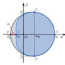
For calculating these parameters, we consider five points $B=\left(\alpha_{t},\beta_{t}\right)$, $D=\left(\alpha_{b},\beta_{b}\right)$, $C=\left(\alpha_{r},0\right)$, $A=\left(\alpha_{p},0\right)$, and $F=\left(\bar{\alpha}_{p},0\right)$, which are top, bottom, rightmost, leftmost of the shadow and leftmost of the reference circle respectively, so we have

	$\displaystyle R_{s}$	$\displaystyle=$	$\displaystyle\frac{\left(\alpha_{t}-\alpha_{r}\right)^{2}+\beta_{t}^{2}}{2\left(\alpha_{t}-\alpha_{r}\right)}\ ,$
	$\displaystyle\delta_{s}$	$\displaystyle=$	$\displaystyle\frac{\left(\bar{\alpha}_{p}-\alpha_{p}\right)}{R_{s}}.$		(52)

From the plots show that the increase in $b$ for a fixed value $l$ and $a$ , leads to a decrease in $R_{s}$, and increases in $\delta_{s}$. For fixed values of $b$, and $a$ both $R_{s}$ and $\delta_{s}$ increases but the nature of variation differs for different values of $a$. Thus the Lorentz Violating term has a significant impact on the size of the shadow and its deviation from the circular form. For all the plots, we have taken $M=1$ for convenience.

We proceed in this Sec. with study the possible visibility of the Kerr-Sen like black-hole through shadow. In the vicinity of limiting constant value, the absorption cross-section of the black-hole moderates lightly at high energy. We know that a rotating black-hole can absorb electromagnetic waves, so the absorbing cross-section BM for a spherically symmetric black-hole is.

$$\sigma_{lim}=\pi R_{s}^{2}.$$

(53)

Using the equation (53) we find out the energy emission rate following the article AA

$$\frac{d^{2}E}{d\omega dt}=\frac{2\pi R_{s}^{2}}{e^{\left(\frac{\omega}{T}\right)}-1}\omega^{3}$$

(54)

where $T$ is the Hawking temperature, $\omega$ the frequency of radiation and $E$ stands for energy.

We have sketched the energy emission rate versus $\omega$ for various cases. It is clear from the sketch that the emission rate decreases with an increase in $b$ for any set of fixed values of $a$ and $\ell$. It also decreases when $\ell$ increases for any set of fixed values of $a$ and $b$. However, there is a crucial difference in the situation when $\ell$ increases. It is true that emission rate decreases with the increase in $\ell$ like the case when $b$ increases but unlike the situation when $b$ increases the pick of the curve gets shifted when $\ell$ increases.

We have considered the Einstein-bumblebee gravity model where LV scenario gets involved through a bumblebee field vector field $B_{\mu}$. A spontaneous symmetry breaking allows the field to acquires a vacuum expectation value that generates LV into the system. A Kerr-Sen-like solution has been found out starting from the generalized form of a radiating stationery axially symmetric black-hole metric. For the parameter $b=0$ the matric turns into Kerr-like metric and for both $b=0$ and $a=0$ the metric lands onto Schwarzschild-like metric. The effective potential that results from the null geodesics in the bumblebee rotating black-hole spacetime is computed that in turn helps to get the tentative nature of the motion of photon is predicted for different choices of the parameters $a$, $b$ and $\ell$. The nature of shadow is studied and how does the shadow gets deformed that has also been studied for different variations of $a$, $b$, and $\ell$. We observe that shadow gets shifted towards the right for positive $\ell$ and shifted towards left for negative $\ell$ when $a$ and $b$ remains fixed. However, shifting is always towards the right when $bl$ increases whatever the set of values of $\ell$ and $a$ are taken. We have also studied the rate of emission of energy for this type of black-hole. The emission rate decreases when $b$ increases for any set of fixed values of $a$ and $\ell$. It also decreases when $\ell$ increases for an arbitrary set of fixed values of $a$ and $b$. A crucial difference however in the situation is noticed when $\ell$ increases. The emission rate although decrease with the increase of $\ell$ like the case when $b$ increases, the pick of the curve gets shifted towards lower $\omega$ in the situation when $\ell$ increases. The deformation of the shadow for Kerr-Sen-like black-hole in the Einstein-bumblebee gravity model with the variation of $\ell$ observed here is a theoretical prediction. It shows that it enhances the distortion of shadow, and it would be detected by the new generation gravitational antennas.

References

- (1) B. P. Abbott et al, Phys. Rev. Lett. 116, 061102 (2016).
- (2) Event Horizon Telescope Collaboration, Astrophys. J. 875, L1 (2019),
- (3) Event Horizon Telescope Collaboration, Astrophys. J, 875(1), L4, (2019)
- (4) V. A. Kostelecky and S. Samuel, Phys. Rev. D39 683 (1989);
- (5) V. A. Kostelecky and S. Samuel, Phys. Rev. Lett. 63, 224 (1989)
- (6) V. A. Kostelecky and S. SamuelPhys. Rev. D 40, 1886 (1989).
- (7) D. Colladay and V. A. Kostelecky, Phys. Rev. D 55, 6760 (1997).
- (8) S. M. Carroll, J. A. Harvey, V. A. Kostelecky, C. D. Lane, T. Okamoto, Phys. Rev. Lett. 87, 141601 (2001).
- (9) R. Gambini, Jorge Pullin, Phys. Rev. D 59, 124021 (1999)
- (10) John Ellis, N. E. Mavromatos, D. V.Nanopoulos, Gen. Rel. Grav. 32, 127 (2000).
- (11) W.-M. Dai, Z.-K. Guo, R.-G. Cai and Y.-Z. Zhang, Eur. Phys. J. C 77 386 (2017)
- (12) V. A. Kostelecky, Phys. Rev. D 69, 105009 (2004).
- (13) G. Rubtsov, P. Satunin, S. Sibiryakov, J. Cosmo. Astro. Phys. (JCAP) 05, 049 (2017)
- (14) D. Colladay, V.A. Kostelecky, Phys. Rev. D 55, 6760 (1997)
- (15) D. Colladay, V.A. Kostelecky, Phys. Rev. D 58, 116002 (1998)
- (16) V.A. Kostelecky, Phys. Rev. D 69, 105009 (2004)
- (17) K. Bakke and H. Belich, Eur. Phys. J. Plus 129: 147 (2014)
- (18) V. A. Kostelecky and C. D. Lane, Journal of Mathematical Physics 40, 6245 (1999).
- (19) T. J. Yoder and G. S. Adkins, Phys. Rev. D 86, 116005 (2012)
- (20) R. Lehnert, Phys. Rev. D 68, 085003 (2003).
- (21) O. G. Kharlanov, V. Ch. Zhukovsky, J. Math. Phys. 48, 092302 (2007).
- (22) V. A. Kostelecky and M. Mewes, Phys. Rev. Lett. 87, 251304 (2001)
- (23) V. A. Kostelecky and M. Mewes, Phys. Rev. D 66, 056005 (2002)
- (24) V. A. Kostelecky and M. Mewes, Phys. Rev. Lett. 97, 140401 (2006)
- (25) V. A. Kostelecky and M. Mewes, Phys. Rev. Lett. 87, 251304 (2001)
- (26) S. Carroll, G.B. Field and R. Jackiw, Phys. Rev. D 41, 1231 (1990)
- (27) C. Adam and F. R. Klinkhamer, Nucl. Phys. B 607, 247 (2001)
- (28) W. F. Chen and G. Kunstatter, Phys. Rev. D 62, 105029 (2000)
- (29) C. D. Carone, M. Sher, and M. Vanderhaeghen, Phys. Rev. D74, 077901 (2006)
- (30) F.R. Klinkhamer and M. Schreck, Nucl. Phys. B848, 90 (2011)
- (31) M. Schreck, Phys. Rev. D 86, 065038 (2012);
- (32) M. A. Hohensee, R. Lehnert, D. F. Phillips, and R. L. Walsworth, Phys. Rev. D 80, 036010 (2009).
- (33) B. Altschul and V. A. Kostelecky, Phys. Lett. B 628, 106
- (34) D. Colladay and P. McDonald, Phys. Rev. D 79, 125019 (2009)
- (35) V. E. Mouchrek-Santos and M. M. Ferreira, Jr., Phys. Rev. D 95, 071701(R) (2017)
- (36) R. Bluhm, V. Alan Kostelecky, Phys. Rev. D 71, 065008 (2005).
- (37) A. F. Santos et al, Mod. Phys. Lett. A 30, 1550011 (2015).
- (38) R. V. Maluf, Victor Santos, W. T. Cruz, and C. A. S. Almeida Phys. Rev. D 88, 025005 (2013).
- (39) Maluf, R.V. et al. Phys. Rev. D 90 (2014) no.2, 025007.
- (40) Q. G. Bailey and V. A. Kostelecky, Phys. Rev. D 74, 045001 (2006).
- (41) V. A. Kostelecky, A. C. Melissinos and M. Mewes, Phys. Lett. B 761, 1 (2016)
- (42) V. A. Kostelecky and M. Mewes, Phys. Lett. B 757, 510 (2016).
- (43) R. P. Kerr, Phys. Rev. Lett. 11, 237 (1963).
- (44) A. Sen Phys. Rev. Lett. 69 (1992) 1006
- (45) E. T. Newman, E. Couch, K. Chinnapared, A. Exton, A. Prakash, R. Torrence J. Math. Phys. 6 918 (1965)
- (46) C. Ding, C. Lui, R. Casana, A. Cavalcante Euro. phys. J. C80 178 2020.
- (47) R. Casana and A. Cavalcante, Phys. Rev. D 97, 104001 (2018).
- (48) Rong-Jia Yang, He Gao, Yao-Guang Zheng, Wu Qin, Commun. Theor. Phys. 71, 568 (2019)
- (49) A. H. Klotz, Gen. Gel. Grav. 14, 727 (1982)
- (50) Y. X. Gui, J. G. Zhang, Y. Zhang and F. P. Chen, Acta Phys. Sin. 33, 1129 (1984).
- (51) R. M. Wald, Phys. Rev. D 48, R3427 (1993).
- (52) J. L. Synge Monthly Notices of the Royal Astronomical Society, 131(3): 463 466, 1966.
- (53) J. M. Bardeen, W. H. Press and S. A. Teukolsky, Astro-phys. J. 178, 347 (1972).
- (54) K. Hioki and K. I. Maeda, Phys. Rev. D 80, 024042 (2009)
- (55) X. G. Lan. and J. Pu: Mod. Phys. Lett A33, 1850099 (2018)
- (56) Shao-Wen Wei, Yu-Xiao Liu: JCAP 11, 063 (2013)
- (57) A. Abdujabbarov, B. Toshmatov, Z. Stuchlik, B. Ahmedov: Int. Jour. Mod. Phys. D26, 1750051 (2017)
- (58) V. Perlick, O. Y. Tsupko: Phys. Rev. D 95, 104003 (2017)
- (59) F. Atamurotov, B. Ahmedov, A. Abdujabbarov Phys. Rev. D92, 084005 (2015)
- (60) G. Z. Babar, A. Z. Babar, F. Atamurotov:Euro. Phys. Jour. C80, 761 (2020)
- (61) T. Tao, Q. Wu, M. Jamil and K. Jusufi, Phys. Rev. D 100, 044055 (2019).
- (62) S. Dastan, R. Saffari, S. Soroushfar: Shadow of a Kerr-Sen dilaton-axion Black-Hole by
- (63) S. W. Wei, P. Cheng, Y. Zhong and X. N. Zhou, J. Cos. Astro. Phys. 08, 004 (2015).
- (64) P. J. Young, Phys. Rev. D 14, 3281 (1976).
- (65) B. Mashhoon, Phys. Rev. D 7, 2807 (1973)
- (66) A. Abdujabbarov, M. Amir, B. Ahmedov and S. G. Ghosh, Phys. Rev. D 93, no. 10, 104004 (2016)