Improving Scalability of Contrast Pattern Mining for Network Traffic Using Closed Patterns

Elaheh AlipourChavary, Sarah M. Erfani, Christopher Leckie email: ealipourchav@student.unimelb.edu.au, sarah.erfani@unimelb.edu.au, caleckie@unimelb.edu.au Affiliation: The University of Melbourne, Melbourne, Australia.

Abstract.

Contrast pattern mining (CPM) aims to discover patterns whose support increases significantly from a background dataset compared to a target dataset. CPM is particularly useful for characterising changes in evolving systems, e.g., in network traffic analysis to detect unusual activity. While most existing techniques focus on extracting either the whole set of contrast patterns (CPs) or minimal sets, the problem of efficiently finding a relevant subset of CPs, especially in high dimensional datasets, is an open challenge. In this paper, we focus on extracting the most specific set of CPs to discover significant changes between two datasets. Our approach to this problem uses closed patterns to substantially reduce redundant patterns. Our experimental results on several real and emulated network traffic datasets demonstrate that our proposed unsupervised algorithm is up to 100 times faster than an existing approach for CPM on network traffic data (Chavary et al. 2017). In addition, as an application of CPs, we demonstrate that CPM is a highly effective method for detection of meaningful changes in network traffic.

Keywords:

contrast patterns, closed patterns, network traffic analysis

1. Introduction

CPM (also is known as emerging pattern mining (Dong and Li 1999)) is an extension of frequent pattern mining that extracts patterns whose support increases significantly from a background dataset to a target dataset (e.g., from day 1 to day 2) (Dong and Li 1999). In other words, it searches for patterns that correspond to changes in the target dataset with respect to the baseline background dataset. CPM is useful in fields such as data summarization and network traffic analysis (Chavary et al. 2017) to identify changes in a system. However, CPM is computationally expensive since (1) the Apriori property does not hold for CPs, and (2) there are many candidate CPs in large datasets, especially for low support thresholds. Thus a major challenge is how to extract CPs in an efficient manner.

Various techniques have been proposed in the literature for CPM, such as (Fan and Ramamohanarao 2006; Bailey and Loekito 2010; Dong and Li 1999; Seyfi 2018). However, the focus of most of these approaches is either extracting the most general patterns or all possible CPs, and they do not address the problem of redundancy and the computational cost of CPM. Alternatively, to extract a high-quality set of CPs and improve performance (Soulet et al. 2004; Garriga et al. 2008; Li et al. 2007), we can search for the most specific contrast patterns. For example discriminative itemset mining (which has a close relationship with CPM) uses the most specific patterns to extract discriminative itemsets. They use additional constraints such as productivity constraints and confidence-interval constraints to generate patterns (Kameya 2019; Pham et al. 2019).

In this paper, we focus on how to efficiently extract the most specific CPs to discover significant changes between two datasets (e.g., changes in network traffic across two different days). Our approach to this problem uses a compact representation of data, called closed patterns (Pasquier et al. 1999), which are those patterns that have no proper supersets with the same support. By elimination of minimal patterns in our approach, we considerably reduce the overlap between generated patterns, and by reducing the redundant patterns, we substantially improve the scalability of CPM. We propose a new scalable algorithm, called EPClose, to extract CPs directly during closed pattern generation. We call this specific subset of contrast patterns as closed contrast patterns (CCPs). In comparison with work in (Chavary et al. 2017), where CPs are generated by a post-mining process, we derive CPs directly during closed pattern generation. In particular, our aim is to examine whether closed patterns provide an expressive and efficient representation for CPM in practice. We apply our EPClose algorithm to network traffic to investigate whether CCPs are useful for distinguishing attack traffic from normal traffic.

Our experimental results show that although we are extracting the same set of CPs as the work in (Chavary et al. 2017), our proposed algorithm achieves a significant speed-up. In addition, our results demonstrate that CCPs have strong discriminative power in detecting pure patterns, i.e., most changes are either attack or normal traffic, but not a mixture of both. In summary, our main contributions are as follows:

•

We propose a new scalable algorithm, called EPClose to extract the most specific contrast patterns (CCPs) directly from closed patterns.
•

We show that CCPs are an expressive and efficient representation of CPs for network traffic analysis.
•

We evaluate our algorithm and compare its performance with a baseline algorithm (Chavary et al. 2017) on three network traffic datasets. The results demonstrate much better efficiency of our algorithm in comparison with (Chavary et al. 2017).
•

We show the practicality of our algorithm in the application of network traffic summarization on different datasets. Although our CPM approach is unsupervised, our evaluation on several labeled datasets demonstrates the ability of CCPs to capture emerging attack patterns. The results show that derived CCPs are powerful tools for distinguishing the attack traffic from normal traffic.

2. Problem Statement

Let $I=\{i_{1},i_{2},\dotsc,i_{m}\}$ be the set of all distinct items in a dataset D, where D is a set of transactions and a transaction T is a non-empty set of items. A transaction may occur several times in D. An itemset or pattern X is any subset of $I$ . We use the terms itemset and pattern interchangeably throughout this work. An itemset X is contained in a transaction T if $X\subseteq{T}$ . We define $D(X)=\{T\in D|X\subseteq T\}$ .

The count of X in dataset D, denoted as $count_{D}(X)$ , is the number of transactions in dataset D containing pattern X. The support of itemset X is the fraction of transactions in dataset D that contain X and is given by $supp_{D}(X)=\frac{count_{D}(X)}{|D|}$ . An itemset X is frequent in a dataset D if $supp_{D}(X)$ is greater than or equal to a pre-defined threshold $\sigma$ . In the following definitions, let $supp_{i}(X)$ denotes $supp_{D_{i}}(X)$ .

Definition 2.1.

The growth rate of a pattern X for a target dataset $D_{t}$ compared to a background dataset $D_{b}$ is $gr(X,D_{t})=\frac{supp_{t}(X)}{supp_{b}(X)}$ , where $gr(X,D_{t})=0$ if $supp_{t}(X)=supp_{b}(X)=0$ , and $gr(X,D_{t})=\infty$ if $supp_{t}(X)>0$ and $supp_{b}(X)=0$ .

Definition 2.2.

A contrast pattern X is a pattern whose support is significantly different from one dataset to another. Given a growth rate threshold $\rho>1$ , pattern X is a contrast pattern for dataset $D_{t}$ if $gr(X,D_{t})\,\geq\,\rho$ .

For example, suppose we are given two datasets $D_{b}$ and $D_{t}$ shown in Table 1 with five transactions in each dataset. Each transaction is a subset of the itemset $I=\{a,b,c,d,e,f,g\}$ . Also, suppose for all examples of this paper $\sigma=0.4$ and $\rho=1.5$ . We are interested in CPs from the background dataset $D_{b}$ to the target dataset $D_{t}$ . Hence, we need to extract all patterns $X$ whose $gr(X,D_{t})\geq\rho$ . For example, the patterns $\{c,e\}(3:1)$ ¹¹ 1 Given $k\geq 1$ $\{a_{1},a_{2},...a_{k}\}(n:m)$ shows that the pattern $\{a_{1},a_{2},...a_{k}\}$ repeats $n$ times in $D_{t}$ and $m$ times in $D_{b}$ is a CP with $gr=3/1$ and $\{a,b,c,e\}(2:0)$ is another CP with $gr=\infty$ .

An example of FP-tree. — Table 1. Example datasets

$D_{b}$	$D_{t}$
abf	abd
bce	bce
bcfg	abce
bc	be
abd	abce

For extracting CPs, our approach is to use closed patterns, which are those patterns that have no proper supersets with the same support. For a formal definition, we utilize the closure operator $\mathcal{H}$ such that $\mathcal{H}(X,D)=\{\bigcap T|T\in D(X)\}$ . A pattern $X$ is closed if $X=\mathcal{H}(X,D)$ , i.e., a pattern is closed if it is equal to its closure.

Definition 2.3.

Given two datasets $D_{b}$ and $D_{t}$ , with size $n_{b}$ and $n_{t}$ respectively, the minimum support threshold of $\sigma$ , and the growth rate threshold of $\rho>1$ , a pattern X is a CCP from $D_{b}$ to $D_{t}$ if it satisfies the following conditions:

(1) $count_{D_{t}}(X)\geq\sigma n_{t}$ ;

(2) $\mathcal{H}(X,D)=X\;\;\;\;\;\;\;\;\;where\;D=D_{b}\cup D_{t}$ ;

(3) $gr(X,D_{t})\,\geq\,\rho$

The first condition guarantees to eliminate infrequent itemsets w.r.t. the target dataset. The second condition ensures that the pattern is closed and the last condition identifies only CPs.

Problem statement: Given two datasets of $D_{b}$ and $D_{t}$ , the minimum support threshold of $\sigma$ , and the growth rate threshold of $\rho>1$ , how can we extract CCPs efficiently from $D_{b}$ to $D_{t}$ .

For example in Table 1, the pattern $\{c,e\}(3:1)$ is a CP but it is not a CCP, since it does not satisfy condition 2 of Definition 2.3. The closure of this pattern is $\{b,c,e\}(3:1)$ . It implicitly conveys that the pattern $\{c,e\}$ will not appear in a transaction without $\{b\}$ . Therefore, non-closed patterns are considered as redundant. However, the pattern $\{b,c,e\}(3:1)$ is a CCP with $gr=3/1$ . Thus, our aim is to derive all CPs that are also closed.

3. Our Approach: EPClose

In this section, we investigate how to derive CCPs efficiently during closed pattern generation.

3.1. Contrast Pattern Mining

Having a pair of datasets $D_{b}$ and $D_{t}$ , a naive method for extracting CPs from the closed patterns is to first discover all closed patterns of each dataset separately; then, as a post-processing step, match the two sets of closed patterns to find similar patterns in the two datasets and compute their supports; and finally compute the growth rate of similar patterns according to their support to find the collection of CPs (Chavary et al. 2017). However, in large and high-dimensional datasets the matching step is computationally expensive.

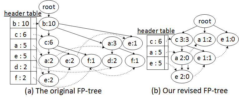
To overcome this problem, we propose an algorithm EPClose, which modifies a closed pattern mining algorithm called FP-close (Grahne and Zhu 2005), such that we can extract CPs directly during closed pattern generation. FP-close is a depth-first algorithm that uses FP-growth (Han et al. 2000) recursively to mine closed frequent itemsets (CFI). An itemset X is a CFI in a dataset D if it is closed and its support is greater than or equal to the minimum support threshold. It uses an efficient data structure called an FP-tree to compress the dataset in memory. However, our revised version of FP-tree has two differences with the original FP-tree. The first difference is that the original FP-tree keeps three fields in each node: item-name, count and node-link. We replace the count with the two counts of background and target datasets separately. The second difference is that the original FP-tree is constructed from all frequent items, while we borrow the concept of full support items (FSIs) from (Pei et al. 2000), and remove FSIs from the FP-tree construction. FSIs are those items that appear in each transaction of a dataset (implicitly they are frequent). However, unlike (Pei et al. 2000), we use it not only for conditional projected datasets(Han et al. 2000), but also for the original dataset used in base FP-tree construction. FSIs have the following property:

{property}

The set of FSIs generates a candidate closed frequent itemset (CFI). If the newly discovered CFI is not a subset of any previously discovered CFI with the same count, it is marked as a CFI.

Join dataset: The FP-close algorithm derives closed patterns from a single dataset, whereas our objective is to compare two datasets and find the differences between them. Thus, we assume that we merge the target dataset $D_{t}$ and the background dataset $D_{b}$ into a single join dataset $D=D_{b}\cup D_{t}$ . By considering the join dataset, all CCPs should not only be frequent in the join dataset, but also should be frequent in the target dataset (the first condition of Definition 2.3).

An example of the original FP-tree and our modified FP-tree is presented in Figure 1, which is constructed from Table 1. Each node corresponds to one item. For each node, we also keep the item counts, separately, for two datasets (Figure 1(b)). It is clear from the figure that the size of our FP-tree is smaller than the original one. The reason is that item $b$ is a FSI, and items $d$ and $f$ are infrequent in $D_{t}$ , so we removed them from our FP-tree. This early pruning can reduce the size of the FP-tree considerably. Please refer to (Han et al. 2000) for details of FP-tree construction.

3.1.1. EPClose Algorithm

Before applying the recursive procedure of EPClose(), the algorithm first scans the join dataset $D=D_{b}\cup D_{t}$ and counts the frequency of each item for $D_{b}$ and $D_{t}$ separately, and saves them in an F-list according to their frequency in descending order. Then, it finds all FSIs from the F-List and according to Property 3.1, marks the set of FSIs as a closed pattern and saves it in a CFI-tree, which is a tree for saving closed patterns. Infrequent items in $D_{t}$ are also removed from the F-list. These two early pruning steps considerably reduce the size of the FP-tree in the EPClose algorithm. The pseudo-code of EPClose is shown in Algorithm 1. The method takes an FP-tree, denoted as FPT, as an input. FPT has two attributes: $FPT.header=\{a_{1},a_{2},\dotsc,a_{k}\}$ and FPT.base. FPT.header is the header table of the FP-tree, and FPT.base is an itemset for which FPT is a conditional FP-tree. In X’s conditional FP-tree, denoted as $FPT_{X}$ , $base$ is equal to the pattern of $X$ .

Data: FPT: FP-tree, C: CFI-tree, FSI: list of full support items,

\sigma

: support threshold,

\rho

: gr threshold

Result: CCP-List: closed contrast patterns list

if FPT only has a single branch B then 2

generate all CFIs from B and FSIs, and call CCP-checking(); 3

else for all item $a_{i}\in FPT.header=\{a_{1},a_{2},\dots,a_{k}\}$ do 4

set

\beta=FPT.base\cup a_{i}

and

betaCount\!=\!min(count_{D}(FPT.base),count_{D}(a_{i}))

; 5

if closed-checking( $\beta\cup FSI$ ,C)==fail then 6

construct

a_{i}

’s conditional pattern base, and count the frequency of items and save in

frequencyMap=\{i_{1},i_{2},\dots,i_{m}\}

; 7

for each item $i_{j}\in frequencyMap$ do 9

if $count_{D}(i_{j})==betaCount$ then 10

insert

i_{j}

FSI_{\beta}

; 11

remove

i_{j}

from frequencyMap; 12

else if $count_{D_{t}}(i_{j})\leq\sigma|D_{t}|$ then 14

remove

i_{j}

from frequencyMap; 15

end if 16

end for 17

copy frequencyMap in F-list; 18

Z=\beta\cup FSI_{\beta}\cup FSI

; 19

if closed-checking(Z,C)==fail then 20

insert Z to C and call CCP-checking(); 21

end if 22

construct

\beta

’s conditional FP-tree

FPT_{\beta}

; 24

if $FPT_{\beta}\neq\emptyset$ then 25

FSI=FSI_{\beta}\cup FSI

; 26

call EPClose(

FPT_{\beta}

, C, FSI,

\sigma

\rho

); 27

end if 28

end if 29

end for 30

ALGORITHM 1 EPClose Algorithm

During the recursion, if FPT has a single branch B, the algorithm generates all CFIs from B and the FSIs according to FP-close, and then applies the CCP-Checking function. This function examines the conditions of Definition 2.3; if pattern $X$ satisfies all conditions, then it is marked as a CCP and saved in the CCP-List along with its corresponding $count_{D_{b}}(X)$ and $count_{D_{t}}(X)$ . If FPT is not a single branch, the algorithm is prepared for another recursive call by constructing $\beta$ ’s conditional FP-tree, denoted as $FPT_{\beta}$ . Unlike FP-close, the EPClose algorithm calls the closed-checking function before constructing $a_{i}$ ’s conditional pattern base, and if $\beta\cup FSI$ passes the closed checking, $a_{i}$ ’s conditional pattern base is constructed. In the closed-checking function, if a pattern does not have any superset with the same support in the CFI-tree C, it will be marked as a closed pattern (Grahne and Zhu 2005).

EPClose saves the dataset distribution information of existing items in the projected database as a hash map, denoted as frequencyMap, in the form of $frequencyMap~=~<key,value>$ according to line 1, where $key$ is an item $i_{j}$ and $value$ is an array of two counts of $i_{j}$ in $D_{b}$ and $D_{t}$ . After this, EPClose finds local FSIs, and moves them from the frequencyMap to a local $FSI_{\beta}$ . Then the algorithm removes all infrequent items from $D_{t}$ , according to line 1. By using these two methods of pruning local FSIs and discarding infrequent items in $D_{t}$ , the size of $FPT_{\beta}$ can be considerably reduced. Finally, before construction of $\beta$ ’s conditional FP-tree, the EPClose algorithm executes an extra closed-checking to determine if the new suffix pattern of $Z=\beta\cup FSI_{\beta}\cup FSI$ is a closed pattern or not. Then the algorithm constructs $\beta$ ’s conditional FP-tree and after merging the local $FSI_{\beta}$ and global FSI, calls the recursive method of EPClose for $FPT_{\beta}$ .

By applying algorithm EPCLose to Table 1, we derive 4 CCPs from all the patterns. They are $\{b,e\}(4:1),\{a,b\}(3:2),\{b,c,e\}(3:1),\{a,b,c,e\}(2:0)$ . The patterns $\{b\}(5:5)$ and $\{b,c\}(3:3)$ are closed patterns, but they are not CCPs, since they do not satisfy condition 3 of Definition 2.3.

4. Experimental Results

To evaluate the efficiency of the proposed EPClose algorithm, we compare it with the ExtCP algorithm (Chavary et al. 2017). For empirical evaluation, three benchmark network traffic datasets are used, namely Kyoto 2006+²² 2 http://www.takakura.com/Kyoto_data/, KDD-CUP 1999³³ 3 http://kdd.ics.uci.edu/databases/kddcup99/kddcup99.html and BGU⁴⁴ 4 https://archive.ics.uci.edu/ml/datasets/detection_of_IoT_
botnet_attacks_N_BaIoT. Kyoto is a real dataset, while the other two are emulated. Table 2 provides the parameters of each dataset. In the Kyoto dataset, we considered the traffic of 15 and 16 July 2007 as the background and target datasets, respectively. For BGU and KDD’99 we randomly select the target and background datasets. The continuous attributes of datasets were discretized by the equal-frequency unsupervised discretization method, and the number of bins in discretization has been given in Table 2. The growth rate threshold is set to 5 for Kyoto and KDD’99 and 1.5 for BGU. All experiments were run in Java on a 2.6GHz CPU with 16GB of memory running Windows 7.

Table 2. Dataset information

Dataset	$\|D_{b}\|$	$\|D_{t}\|$	Attributes	Bins	Items
Kyoto	119702	123835	14	4	108
KDD’99	15000	15000	10	5	38
BGU	4500	4500	23	2	46

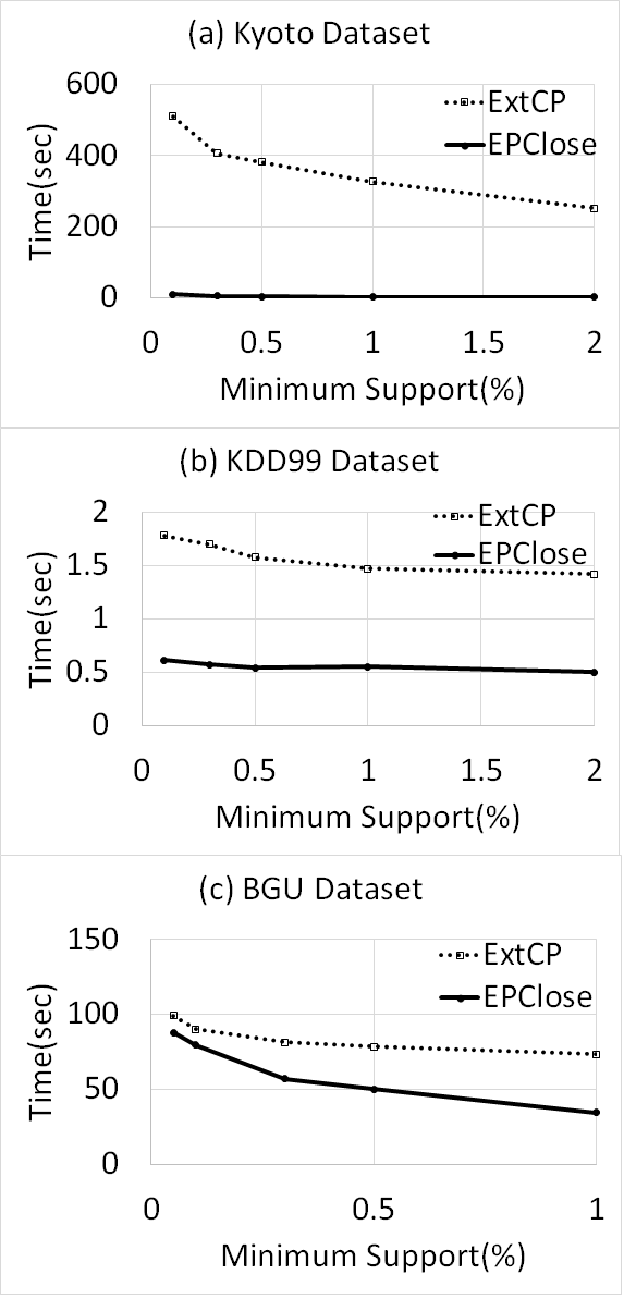
Figure 2. Run time for different datasets.Processing Time for different datasets.

Attack ratio for different datasets. — Figure 2. Run time for different datasets.Processing Time for different datasets.

Figure 3 illustrates the runtime of each algorithm in the three datasets. Although our generated patterns are the same as for ExtCP, our algorithm considerably outperforms it, and obtains speed-up rates of up to 100 over ExtCP. In Kyoto, with minimum support of 0.1 $\%$ , the processing time is only 10 seconds for our algorithm, while this time grows to 500 sec for ExtCP. The reason why this difference is less for the BGU dataset is that BGU was discretized into two bins, causing many duplicate transactions. As a result, the number of generated CCPs reduces. So the cost of matching in ExtCP is comparable to the cost of FP-tree construction.

In Figure 3, we evaluate the quality of extracted CCPs for network traffic analysis. Although our approach for CCP generation is unsupervised, we use the labels in the target dataset for evaluation. Figure 3 shows the attack ratio per CCP for three datasets. Attack ratio is the probability that a CCP belongs to the attack class in the target dataset (Chavary et al. 2017). The derived CCPs are for a minimum support of 0.1%. It is clear from the graphs that a substantial portion of CCPs are pure patterns. In Kyoto, 97 $\%$ of CCPs can uniquely distinguish between classes. This number is 78 $\%$ and 80 $\%$ for KDD’99 and BGU respectively. It is worth noting that the CCPs for Kyoto (which is a real-life dataset) were almost all pure.

5. Conclusion and Future Work

In this paper, we investigated the suitability of closed patterns for CPM. We proposed a new algorithm, called EPClose that uses a revised version of the FP-tree data structure to derive all CCPs directly from the closed patterns. Our experimental results show that EPClose is much faster than the existing ExtCP algorithm. We also show that CCPs have strong discriminative power in detecting pure network traffic patterns. As future work, we will compare the performance of our work with other approaches, and investigate how to efficiently mine CCPs online over data streams.

References

(1)
Bailey and Loekito (2010) James Bailey and Elsa Loekito. 2010. Efficient incremental mining of contrast patterns in changing data. IPL (2010), 88–92.
Chavary et al. (2017) Elaheh Alipour Chavary, Sarah M Erfani, and Christopher Leckie. 2017. Summarizing Significant Changes in Network Traffic Using Contrast Pattern Mining. In CIKM. 2015–2018.
Dong and Li (1999) Guozhu Dong and Jinyan Li. 1999. Efficient mining of emerging patterns: Discovering trends and differences. In SIGKDD. 43–52.
Fan and Ramamohanarao (2006) Hongjian Fan and Kotagiri Ramamohanarao. 2006. Fast discovery and the generalization of strong jumping emerging patterns for building compact and accurate classifiers. TKDE (2006), 721–737.
Garriga et al. (2008) Gemma C Garriga, Petra Kralj, and Nada Lavrač. 2008. Closed sets for labeled data. JMLR (2008), 559–580.
Grahne and Zhu (2005) Gösta Grahne and Jianfei Zhu. 2005. Fast algorithms for frequent itemset mining using fp-trees. TKDE (2005), 1347–1362.
Han et al. (2000) Jiawei Han, Jian Pei, and Yiwen Yin. 2000. Mining frequent patterns without candidate generation. In SIGMOD. 1–12.
Kameya (2019) Yoshitaka Kameya. 2019. Towards efficient discriminative pattern mining in hybrid domains. arXiv (2019).
Li et al. (2007) Jinyan Li, Guimei Liu, and Limsoon Wong. 2007. Mining statistically important equivalence classes and delta-discriminative emerging patterns. In SIGKDD. 430–439.
Pasquier et al. (1999) Nicolas Pasquier, Yves Bastide, Rafik Taouil, and Lotfi Lakhal. 1999. Efficient mining of association rules using closed itemset lattices. IS (1999), 25–46.
Pei et al. (2000) Jian Pei, Jiawei Han, Runying Mao, et al. 2000. CLOSET: An Efficient Algorithm for Mining Frequent Closed Itemsets. In SIGMOD. 21–30.
Pham et al. (2019) Hoang Son Pham, Gwendal Virlet, Dominique Lavenier, and Alexandre Termier. 2019. Statistically Significant Discriminative Patterns Searching. arXiv (2019).
Seyfi (2018) Majid Seyfi. 2018. Mining discriminative itemsets in data streams using different window models. Ph.D. Dissertation. Queensland University of Technology.
Soulet et al. (2004) Arnaud Soulet, Bruno Crémilleux, and François Rioult. 2004. Condensed representation of emerging patterns. In PAKDD. 127–132.