Joint Beamforming Design and Power
Splitting Optimization in IRS-Assisted SWIPT NOMA Networks

In this paper, we consider the downlink transmission in an IRS-assisted SWIPT NOMA network consisting of one BS, one IRS and $K$ users. The set of users is denoted by ${\cal K}=\left\{{1,2,...,K}\right\}$. It can be assumed that the BS is equipped with $N>1$ uniform linear array (ULA) antennas and each user is equipped with one antenna. The IRS is equipped with $M$ ULA reflecting elements¹¹ 1 The proposed optimization algorithm when the IRS is equipped with ULA can be well extended to the setup where the IRS is equipped with uniform planar array (UPA)., denoted by ${\cal M}=\left\{{1,2,...,M}\right\}$. A smart controller is equipped at the IRS to coordinate its switching between two working modes, namely the receiving mode for channel estimation and the reflection mode for signal transmission [46]. Since IRS elements are passively reflective, they are passive devices. We consider the use of time-division duplexing (TDD) protocol for uplink and downlink communication. Combined with the reciprocity of the channel, the downlink channel state information (CSI) can be obtained according to the uplink channel estimation. Thus, we assume the CSI of all channels is perfectly known at the BS²² 2 It is worth noting that although this paper is the design of the optimization algorithm with the assumption that perfect CSI is available at the BS, the framework and process of the proposed optimization algorithm can still be applied to robust optimization algorithm design in the case of imperfect CSI.. Meanwhile, we assume that all channels are quasi-static flat-fading.

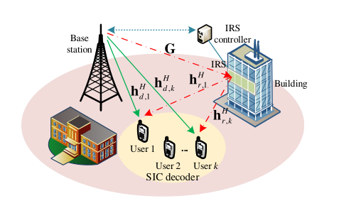
The channel gains from the BS to IRS, from the IRS to $k$-th user, and from the BS to $k$-user are respectively represented by ${\bf{G}}\in{\mathbb{C}^{M\times N}}$, ${\bf{h}}_{r,k}^{H}\in{\mathbb{C}^{1\times M}}$ and ${\bf{h}}_{d,k}^{H}\in{\mathbb{C}^{1\times N}}$, $\forall k\in{\cal K}$. Let ${\bf{\Theta}}={\rm{diag}}\left({{\beta_{1}}{e^{j{\theta_{1}}}},{\beta_{2}}{e^{j{\theta_{2}}}},...,{\beta_{M}}{e^{j{\theta_{M}}}}}\right)\in{\mathbb{C}^{M\times M}}$ denote the reflection coefficients matrix of the IRS, where ${\beta_{m}}\in\left[{0,1}\right]$ and ${\theta_{m}}\in\left[{0,2\pi}\right]$ denote the amplitude reflection coefficient and phase shift of the $m$-th reflecting element, respectively³³ 3 It is worth noting that there are IRS amplitude and phase shift models that are closer to the practical system. In order to characterize the basic performance limit of IRS, we assume that the phase shift varies continuously from 0 to 2$\pi$. In practice systems, we usually choose from a discrete value from 0 to 2$\pi$. Discrete phase shift optimization research will be discussed in the future work. In addition, the amplitude of the IRS can also vary continuously from 0 to 1. In practice, in order to maximize the power of the reflected signal, we usually set $\beta_{m}=1$.. Due to the severe path loss, signals reflected by the IRS twice or more are negligible and can be ignored. In the deployment of actual scenarios, we usually consider that the reflecting element of the IRS is designed to maximize the reflected signal, thus ${\beta_{m}}{\rm{=1,}}\forall m\in{\cal M}$. The wireless channel can be divided into three parts, namely, BS-IRS channel, IRS-user channel, BS-user channel. Although the channel between the BS and users may be blocked, the wireless channel still has a lot of scattering, thus we model the BS-user channel as Rayleigh fading and denote it as ${\bf{g}}_{d,k}^{H}\in{{\mathbb{C}}^{1\times N}}$. We assume that each element of ${\bf{g}}_{d,k}^{H}$ is independent and identically distributed (i.i.d.) CSCG random variable with zero mean and unit variance. Therefore, the channel gain of the BS-user can be expressed as

where $C_{0}$ represents the path loss when the reference distance ${D_{0}}=1\left({\rm{m}}\right)$, ${{d_{d,k}}}$ is the distance from the BS to the $k$-th user, and ${\alpha}_{1}$ represents the path loss exponent.

In addition, for the BS-IRS channel and IRS-user channel, there are LoS components, thus we model them as Rician fading. The BS-IRS channel can be denoted by

where $\kappa$ is the Rician factor, ${{\bf{G}}^{{\rm{LoS}}}}\in{\mathbb{C}^{M\times N}}$ and ${{\bf{G}}^{{\rm{NLoS}}}}\in{\mathbb{C}^{M\times N}}$ are the line-of-sight (LoS) component and non-line-of-sight (NLoS) component, respectively. Each element of ${{\bf{G}}^{{\rm{NLoS}}}}$ is i.i.d. CSCG random variable with zero mean and unit variance. Similarly, the IRS-user channel can be expressed as

where $\vartheta$ is the Rician factor, ${\bf{h}}_{r,k}^{{\rm{LoS}}}\in{\mathbb{C}^{1\times M}}$ and ${\bf{h}}_{r,k}^{{\rm{NLoS}}}\in{\mathbb{C}^{1\times M}}$ are the LoS component and NLoS component, respectively. Each element of ${\bf{h}}_{r,k}^{{\rm{NLoS}}}$ is i.i.d. CSCG random variable with zero mean and unit variance.

The LoS component is represented by the array response of ULA. The array response of $N$ elements ULA can be expressed as

where $\theta$ represents the angle of arrival (AoA) or angle of departure (AoD) of the signal. Therefore, the LoS component ${\bf{G}}^{{\rm{LoS}}}$ can be given by

where ${{\theta_{{\rm{AoA,1}}}}}$ is the AoA to the ULA at the IRS, and ${{\theta_{{\rm{AoD,1}}}}}$ is the AoD from the ULA at the BS. Similarly, the LoS component ${\bf{h}}_{r,k}^{{\rm{LoS}}}$ can be expressed as

where ${{\theta_{{\rm{AoD,2}}}}}$ is the AoD from the ULA at the IRS.

Therefore, the channel gain of BS-IRS and IRS-user can be expressed as

and

where ${{d_{d,r}}}$ and ${{d_{r,k}}}$ represent the distance from the BS to the IRS and the distance from the IRS to the $k$-th user, respectively. ${\alpha}_{2}$ and ${\alpha}_{3}$ respectively represent the path loss exponent from BS to IRS and IRS to the $k$-th user.

In this paper, we assume linear transmit precoding at BS, where each user is assigned with one dedicated information beam. Therefore, the complex baseband transmitted signal at BS can be expressed as

where ${s_{k}}$ denotes the transmission data symbol for the $k$-th user, and ${{\bf{w}}_{k}}\in{\mathbb{C}^{N\times 1}}$ represents the corresponding beamforming vector. We assume that ${s_{k}}$ is i.i.d. CSCG random variables with zero mean and unit variance, denoted by ${s_{k}}\sim{\cal C}{\cal N}\left({0,1}\right),\forall k\in{\cal K}$.

The received signal at the $k$-th user from both the BS-user link and BS-IRS-user link can be expressed as

where ${n_{k}}\sim{\cal C}{\cal N}\left({0,\sigma_{k}^{2}}\right)$ denotes the antenna noise at the $k$-th user.

In addition, we consider that each user applies PS scheme to coordinate the process of information decoding and energy harvested from the received signal [15]. The PS receiver architecture is shown in Fig. 2. The received signal at each user is split to the information decoder (ID) and the energy harvester (EH) by a power splitter. For the $k$-th user, it divides ${\rho_{k}}\left({0\leq{\rho_{k}}\leq 1}\right)$ portion of the signal power to the ID, remaining $1-{\rho_{k}}$ portion of the signal power to the EH. Therefore, the signal split to the ID for $k$-th user can be given by

where ${z_{k}}\sim{\cal C}{\cal N}\left({0,\delta_{k}^{2}}\right)$ is the additional noise introduced by the ID at the $k$-th user.

Since we consider NOMA transmission, the SIC decoding order is very important, which is determined by the channel conditions. Unlike the general NOMA communication system, the combination of IRS and NOMA makes the channel more complicated, because the channel gain may change due to the change of the IRS phase shift matrix. Let $s\left(k\right)$ denote the decoding order for the $k$-th user. Then, $s\left(k\right)=i$ denotes that the $k$-th user is the $i$-th signal to be decoded at the receiver. Accordingly, the signal to interference-plus-noise-ratio (SINR) of the $k$-th user can be expressed as

It is assumed that $s\left(k\right)\leq s\left({\bar{k}}\right)$, the SINR of the $\bar{k}$-th user decoding information signal of the $k$-th user can be given by

In order to ensure that the $\bar{k}$-th user can decode the information of the $k$-th user with the decoding order $s\left(k\right)\leq s\left({\bar{k}}\right)$, the SIC decoding condition ${\rm{SIN}}{{\rm{R}}_{k}}\leq{\rm{SIN}}{{\rm{R}}_{\bar{k}\to k}}$ should be satisfied [47]. For example, supposing the decoding order of the three users is $s\left(k\right)=i,i=1,2,3$. Therefore, the SIC decoding conditions at user 2 and user 3 should satisfy the following conditions: ${\rm{SIN}}{{\rm{R}}_{2\to 1}}\geq{\rm{SIN}}{{\rm{R}}_{1}}$, ${\rm{SIN}}{{\rm{R}}_{3\to 1}}\geq{\rm{SIN}}{{\rm{R}}_{1}}$ and ${\rm{SIN}}{{\rm{R}}_{3\to 2}}\geq{\rm{SIN}}{{\rm{R}}_{2}}$.

In addition, the signal split to the EH for the $k$-th user can be expressed as

Then, the harvested power by the EH for the $k$-th user can be given by

where ${\eta_{k}}\in\left({0,1}\right]$ denotes the power conversion efficiency at EH of the $k$-th user. In this paper, we consider the normalized time, then the harvested power is the harvested energy.

In this paper, we aim to minimize the BS transmit power by jointly designing SIC decoding order, BS transmit beamforming vector, received PS ratio and IRS phase shift matrix. Accordingly, the problem can be formulated as follows,

where constraint (16b) guarantees the QoS requirement of the $k$-th user with the SINR threshold ${\gamma_{k}}$. Meanwhile, constraint (16c) ensures SIC decoding conditions. In addition, constraint (16d) requires that the energy harvested of the $k$-th user needs to reach a threshold ${e_{k}}$. Considering that each user should have non-zero SINR threshold and energy harvested threshold, i.e., ${\gamma_{k}}>0$ and ${e_{k}}>0$, the received PS ratio of the $k$-th user should satisfy constraint (16e). Constraint (16f) is the condition that IRS phase shift should meet. $\Omega$ in constraint (16g) is the combination set of all possible SIC decoding orders.

It can be seen that the problem (P1) is a non-convex optimization problem due to the following reasons. Firstly, the BS transmit beamforming, received PS ratio and IRS phase shift matrix are highly coupled. In addition, the phase shift is expressed in exponential form. Finally, the SIC decoding orders are determined by the IRS phase shift, thus the SIC decoding order and the IRS phase shift are also related. Therefore, it is challenging to directly solve this problem.

In this subsection, the SIC decoding order determination algorithm based on the combined channel gains is proposed. Since this paper considers NOMA, the SIC decoding order is a factor that must be considered. In fact, the SIC decoding order is determined by the channel gain from the BS to each user. Due to the addition of IRS, the SIC decoding order is not only determined by the direct channel gain from the BS to the ground user, but by the combined channel gain from the BS to each user. The change of the IRS phase shift matrix will influence the combined channel gain. Since the same phase shift is different for all users, the combined channel gain of different users cannot be maximized at the same time. Therefore, we maximize sum of the combined channel gain from the BS to all users by optimizing the IRS phase shift. We can sort the combined channel gains of all users to determine the SIC decoding order. The problem of maximizing the sum of the combined channel gains of all users can be expressed as

where ${\bf{\Theta}}={\rm{diag}}\left({{e^{j{\theta_{1}}}},{e^{j{\theta_{2}}}},...,{e^{j{\theta_{M}}}}}\right)$. Let ${u_{m}}={e^{j{\theta_{m}}}},\forall m\in{\cal M}$, ${\bf{u}}={\left[{{u_{1}},{u_{2}},...,{u_{M}}}\right]^{H}}\in{\mathbb{C}^{M\times 1}}$. Then the constraint on ${\theta_{m}}$ is equivalent to $\left|{{u_{m}}}\right|=1,\forall m\in{\cal M}$. Let ${{\bf{a}}_{k}}={\rm{diag}}\left({{\bf{h}}_{r,k}^{H}}\right){\bf{G}}\in{\mathbb{C}^{M\times N}}$, then ${\left\|{{\bf{h}}_{r,k}^{H}{\bf{\Theta G}}+{\bf{h}}_{d,k}^{H}}\right\|^{2}}$ can be written as ${\left\|{{{\bf{u}}^{H}}{{\bf{a}}_{k}}+{\bf{h}}_{d,k}^{H}}\right\|^{2}}$. We introduce auxiliary variables as follows,

Therefore, ${\left\|{{{\bf{u}}^{H}}{{\bf{a}}_{k}}+{\bf{h}}_{d,k}^{H}}\right\|^{2}}$ can be further expressed as ${{\bf{\bar{u}}}^{H}}{{\bf{R}}_{k}}{\bf{\bar{u}}}+{\left\|{{\bf{h}}_{d,k}^{H}}\right\|^{\rm{2}}}$. Since ${{\bf{\bar{u}}}^{H}}{{\bf{R}}_{k}}{\bf{\bar{u}}}={\rm{Tr}}\left({{{\bf{R}}_{k}}{\bf{\bar{u}}}{{{\bf{\bar{u}}}}^{H}}}\right)$, we define ${\bf{\bar{U}}}={\bf{\bar{u}}}{{\bf{\bar{u}}}^{H}}$, where ${\bf{\bar{U}}}\succeq 0$ and ${\rm{Rank}}\left({\bf{\bar{U}}}\right)=1$. Since the rank-one constraint is non-convex, we use SDR to relax this constraint firstly, and the problem (P2) can be transformed into

The above problem (P2.1) is a standard semidefinite programming (SDP) problem, which can be solved by using CVX toolbox [48]. The problem (P2.1) is equivalent to the problem (P2) if and only if the optimal solution ${\bf{\bar{U}}}^{*}$ of the problem (P2.1) is a rank-one matrix. However, under normal circumstances, the problem (P2.1) generally does not produce a rank-one solution, i.e., ${\rm{Rank}}\left({\bf{\bar{U}}}\right)\neq 1$. The optimal solution of problem (P2.1) is only the upper bound of problem (P2), so it is necessary to reconstruct the high-rank solution obtained from problem (P2.1) into a rank-one solution. In this paper, we use Gaussian randomization to reduce the rank of high-rank solution. Since ${\rm{Rank}}\left({\bf{\bar{U}}}\right)\neq 1$, the eigenvalue decomposition of ${\bf{\bar{U}}}$ can be expressed as

where ${\bf{V}}=\left[{{e_{1}},{e_{2}},...,{e_{M+1}}}\right]$ is the identity matrix of the eigenvector, and ${\bf{\Sigma}}{\rm{=diag}}\left({{\lambda_{\rm{1}}},{\lambda_{2}},...,{\lambda_{M+1}}}\right)$ is the diagonal matrix of the eigenvalue. Next, we generate two independent zero-mean normal distribution random vectors ${\bf{\alpha}}\in{\mathbb{R}^{\left({M+1}\right)\times 1}}$, ${\bf{\beta}}\in{\mathbb{R}^{\left({M+1}\right)\times 1}}$ and covariance matrix $\frac{1}{2}{{\bf{I}}_{M+1}}$. Let $T$ be the maximum generation of candidate random variables. The Gaussian random vector of the $t$-th generation can be expressed as

where $\bf{\alpha}_{t}$ and $\bf{\beta}_{t}$ are the $t$-th generation random vectors. Based on the obtained Gaussian random vector ${{\bf{r}}_{t}}\sim{\cal C}{\cal N}\left({{\bf{0}},{{\bf{I}}_{M+1}}}\right)$, we can obtain the suboptimal solution of the problem (P2.1), which can be expressed as

Therefore, the candidate reflection matrix can be expressed as

where ${{\bf{\bar{u}}}_{t}}\left[m\right]$ represents the $m$-th reflecting element of ${{\bf{\bar{u}}}_{t}}$. According to the obtained candidate reflection matrix set $\left\{{\left.{{{\bf{\Theta}}_{t}}}\right|t=1,2,...,T}\right\}$, we can obtain the one that maximizes the combined channel gain of all users, i.e.,

It has been verified that SDR technique followed by such randomization scheme can guarantee at least a $\pi/4$-approximation of the optimal objective value of the problem (P2) [17].

Let ${\bf{h}}_{k}^{H}={\bf{h}}_{r,k}^{H}{\bf{\Theta G}}+{\bf{h}}_{d,k}^{H}\in{\mathbb{C}^{1\times N}}$. Based on the SIC decoding order obtained in the first stage, and given PS ratio IRS phase shift, the problem (P1) can be transformed into the problem (P3), which can be expressed as

Define ${{\bf{W}}_{k}}{\rm{=}}{{\bf{w}}_{k}}{\bf{w}}_{k}^{H}\in{\mathbb{C}^{N\times N}},\forall k$, and ${{\bf{W}}_{k}}$ satisfies ${\rm{Rank}}\left({{{\bf{W}}_{k}}}\right)={\rm{1}},\forall k$. We first apply SDR to relax the rank-one constraint, the problem (P3) can be transformed into the problem (P3.1), which can be expressed as

Since the constraint (26c) is non-convex, the problem (P3.1) is still a non-convex optimization problem. In this paper, we use SCA to convert the constraint (26c) into

where ${{\bf{W}}_{k}^{\left(r\right)}}$ is the value of ${\bf{W}}_{k}$ for the $r$-th iteration. See Appendix A for ${\hat{f}_{1}}\left({{{\bf{W}}_{k}}}\right)$ and ${\hat{f}_{2}}\left({{{\bf{W}}_{j}}}\right)$.

Please refer to Appendix A for the detailed proof. $\hfill\blacksquare$

Accordingly, the problem (P3.1) can be transformed into the problem (P3.2), which can be expressed as

The problem (P3.2) is a standard SDP problem, which can be solved by applying the CVX toolbox [48]. We assume that ${\bf{W}}_{k}^{*}$ is the optimal solution of the problem (P3.2). If ${\bf{W}}_{k}^{*}$ satisfies ${\rm{Rank}}\left({{\bf{W}}_{k}^{*}}\right)=1,\forall k$, the beamforming vector ${\bf{w}}_{k}^{*}$ of the problem (P3) can be obtained by eigenvalue decomposition. Next, we have the following proposition.

Proposition 1: The optimal solution ${\bf{W}}_{k}^{*}$ of the problem (P3.2) satisfies ${\rm{Rank}}\left({{\bf{W}}_{k}^{*}}\right)=1,\forall k$, i.e., the SDR for the problem (P3) is tight.

Please refer to Appendix B for the detailed proof.$\hfill\blacksquare$

In this sub-problem, according to the SIC decoding order obtained in the first stage, given BS beamforming vector and IRS phase shift, the problem (P1) can be transformed into a feasibility-check problem (P4), which can be given by

Due to the existence of the non-convex constraint (29c), the problem (P4) is a non-convex optimization problem. By applying SCA, the constraint (29c) is transformed into

where $\rho_{k}^{\left(r\right)}$ is the value of $\rho_{k}$ for the $r$-th iteration.

Please refer to the Appendix C for detailed proof. $\hfill\blacksquare$

Thus, the problem (P4) can be rewritten as

It can be seen that the problem (P4.1) is a standard convex optimization problem, which can be solved by applying the CVX toolbox [48].

When the SIC decoding order is determined, and beamforming vector and PS ratio are fixed, according to the variable substitution ${\bf{u}}{\rm{=}}{\left[{{e^{j{\theta_{1}}}},...,{e^{j{\theta_{M}}}}}\right]^{H}}\in{\mathbb{C}^{M\times 1}}$ in Section III.A, the constraint on ${\theta_{m}}$ can be transformed into $\left|{{u_{m}}}\right|=1,\forall m\in{\cal M}$. Let ${{\bf{p}}_{k,j}}={\rm{diag}}\left({{\bf{h}}_{r,j}^{H}}\right){\bf{G}}{{\bf{w}}_{k}}\in{\mathbb{C}^{M\times 1}}$, ${{\bf{q}}_{k,j}}={\bf{h}}_{d,j}^{H}{{\bf{w}}_{k}}\in\mathbb{C}$. Then ${\left|{\left({{\bf{h}}_{r,j}^{H}{\bf{\Theta G}}+{\bf{h}}_{d,j}^{H}}\right){{\bf{w}}_{k}}}\right|^{2}}={\left|{{{\bf{u}}^{H}}{{\bf{p}}_{k,j}}+{{\bf{q}}_{k,j}}}\right|^{2}}$. Next we introduce auxiliary variables as follows,

Then ${\left|{{{\bf{u}}^{H}}{{\bf{p}}_{k,j}}+{{\bf{q}}_{k,j}}}\right|^{2}}={{\bf{\bar{u}}}^{H}}{{\bf{S}}_{k,j}}{\bf{\bar{u}}}+{\left|{{{\bf{q}}_{k,j}}}\right|^{2}}$. Since ${{\bf{\bar{u}}}^{H}}{{\bf{S}}_{k,j}}{\bf{\bar{u}}}={\rm{Tr}}\left({{{\bf{S}}_{k,j}}{\bf{\bar{u}}}{{{\bf{\bar{u}}}}^{H}}}\right)$, we define ${\bf{\bar{U}}}{\rm{=}}{\bf{\bar{u}}}{{\bf{\bar{u}}}^{H}}$, where ${\bf{\bar{U}}}$ satisfies ${\bf{\bar{U}}}\succeq 0$ and ${\rm{Rank}}\left({\bf{\bar{U}}}\right)=1$. Since rank-one constraint is non-convex constraint, we firstly apply the SDR to relax it. Because the objective function of the problem (P1) does not contain the IRS phase shift variable, the problem (P1) is transformed into a feasibility-check problem (P5), which can be expressed as

We apply SCA to transform the non-convex constraint (33c) into

where ${{{{\bf{\bar{U}}}}^{\left(r\right)}}}$ is the value of ${{\bf{\bar{U}}}}$ for the $r$-th iteration. See Appendix D for ${{\hat{g}}_{1}}\left({{\bf{\bar{U}}}}\right)$ and ${{\hat{g}}_{2}}\left({{\bf{\bar{U}}}}\right)$.

Please refer to Appendix D for the detailed proof. $\hfill\blacksquare$

Thus, the problem (P5) can be transformed into the problem (P5.1), which can be expressed as

The problem (P5.1) is a standard SDP programming problem, which can be solved by CVX toolbox [48]. In general, problem (P5.1) does not produce a rank-one solution, i.e., ${\rm{Rank}}\left({\bf{U}}\right)\neq 1$. The optimal solution obtained by the problem (P5.1) is only the upper bound of the optimal solution. Therefore, it is necessary to reconstruct the high-rank solution obtained in problem (P5.1) into a rank-one solution, i.e., to reduce the rank of the high-rank solution by using the Gaussian randomization in the subsection III.A.

Based on the previous sub-sections, the two-stage overall optimization algorithm is summarized as Algorithm 1 (i.e. JDBPR algorithm). Specifically, in the first stage, the SIC decoding order is determined by solving the problem (P2), which mainly optimizes the IRS phase shift matrix to maximize the combined channel gain of all users, and then determines the decoding order according to the combined channel gain of each user. Based on the SIC decoding order obtained in the first stage, when PS ratio and IRS phase shift are fixed in the second stage, the BS beamforming vector is obtained by solving the problem (P3) by applying SDR and SCA, and SDR is proved tight. Next, the last two sub-problems of PS ratio and IRS phase shift can be obtained by solving problem (P4) and (P5) by using SDR, SCA and Gaussian randomization when BS transmit beamforming vector is given. The three sub-problems of the second stage are alternately optimized to achieve convergence⁴⁴ 4 For the two-stage overall optimization algorithm (i.e., JDBPR algorithm) proposed in this paper, the Gaussian randomization used in the first stage can obtain an approximate value of at least $\pi/4$ for the optimal objective value of this stage. Meanwhile, for the three sub-problems of the second stage, since each of the three sub-problems has a complex SIC decoding condition constraint, we apply SCA to solve these sub-problems. Therefore, the JDBPR algorithm can obtain a sub-optimal solution of the problem (P1).

References

- [1] Q. Wu and R. Zhang, “Towards smart and reconfigurable environment: Intelligent reflecting surface aided wireless network,” IEEE Commun. Mag., vol. 58, no. 1, pp. 106–112, 2020.
- [2] W. Ni, X. Liu, Y. Liu, H. Tian, and Y. Chen, “Resource allocation for multi-cell IRS-aided NOMA networks,” arXiv preprint arXiv:2006.11811, 2020.
- [3] L. Lu, G. Y. Li, A. L. Swindlehurst, A. Ashikhmin, and R. Zhang, “An overview of massive MIMO: Benefits and challenges,” IEEE J. Sel. Topics Signal Process., vol. 8, no. 5, pp. 742–758, 2014.
- [4] Q. Wu, W. Chen, M. Tao, J. Li, H. Tang, and J. Wu, “Resource allocation for joint transmitter and receiver energy efficiency maximization in downlink OFDMA systems,” IEEE Trans. Commun., vol. 63, no. 2, pp. 416–430, 2015.
- [5] Y. Liu, Z. Qin, M. Elkashlan, Z. Ding, A. Nallanathan, and L. Hanzo, “Non-orthogonal multiple access for 5G and beyond,” Proc. IEEE, vol. 105, no. 12, pp. 2347–2381, 2017.
- [6] L. Dai, B. Wang, Y. Yuan, S. Han, I. Chih-lin, and Z. Wang, “Non-orthogonal multiple access for 5g: solutions, challenges, opportunities, and future research trends,” IEEE Commun. Mag., vol. 53, no. 9, pp. 74–81, 2015.
- [7] Y. Zhou, V. W. S. Wong, and R. Schober, “Coverage and rate analysis of millimeter wave NOMA networks with beam misalignment,” IEEE Trans. Wireless Commun., vol. 17, no. 12, pp. 8211–8227, 2018.
- [8] F. Wei and W. Chen, “Low complexity iterative receiver design for sparse code multiple access,” IEEE Trans. Commun., vol. 65, no. 2, pp. 621–634, 2017.
- [9] Y. Feng, S. Yan, Z. Yang, N. Yang, and J. Yuan, “Beamforming design and power allocation for secure transmission with NOMA,” IEEE Trans. Wireless Commun., vol. 18, no. 5, pp. 2639–2651, 2019.
- [10] Y. Cai, Z. Qin, F. Cui, G. Y. Li, and J. A. McCann, “Modulation and multiple access for 5G networks,” IEEE Communications Surveys Tutorials, vol. 20, no. 1, pp. 629–646, 2018.
- [11] Z. Ding, Y. Liu, J. Choi, Q. Sun, M. Elkashlan, I. Chih-Lin, and H. V. Poor, “Application of non-orthogonal multiple access in LTE and 5G networks,” IEEE Commun. Mag., vol. 55, no. 2, pp. 185–191, 2017.
- [12] Z. Ding, P. Fan, and H. V. Poor, “Impact of user pairing on 5G nonorthogonal multiple-access downlink transmissions,” IEEE Trans. Veh. Technol., vol. 65, no. 8, pp. 6010–6023, 2016.
- [13] Y. Zeng, B. Clerckx, and R. Zhang, “Communications and signals design for wireless power transmission,” IEEE Trans. Commun., vol. 65, no. 5, pp. 2264–2290, 2017.
- [14] B. Clerckx, R. Zhang, R. Schober, D. W. K. Ng, D. I. Kim, and H. V. Poor, “Fundamentals of wireless information and power transfer: From RF energy harvester models to signal and system designs,” IEEE J. Sel. Areas Commun., vol. 37, no. 1, pp. 4–33, 2019.
- [15] Q. Shi, L. Liu, W. Xu, and R. Zhang, “Joint transmit beamforming and receive power splitting for MISO SWIPT systems,” IEEE Trans. Wireless Commun., vol. 13, no. 6, pp. 3269–3280, 2014.
- [16] X. Zhou, R. Zhang, and C. K. Ho, “Wireless information and power transfer: Architecture design and rate-energy tradeoff,” IEEE Trans. Commun., vol. 61, no. 11, pp. 4754–4767, 2013.
- [17] Q. Wu and R. Zhang, “Intelligent reflecting surface enhanced wireless network via joint active and passive beamforming,” IEEE Trans. Wireless Commun., vol. 18, no. 11, pp. 5394–5409, 2019.
- [18] Q. Wu and R. Zhang, “Beamforming optimization for wireless network aided by intelligent reflecting surface with discrete phase shifts,” IEEE Trans. Commun., vol. 68, no. 3, pp. 1838–1851, 2020.
- [19] W. Tang, M. Z. Chen, J. Y. Dai, Y. Zeng, X. Zhao, S. Jin, Q. Cheng, and T. J. Cui, “Wireless communications with programmable metasurface: New paradigms, opportunities, and challenges on transceiver design,” IEEE Wireless Commun., vol. 27, no. 2, pp. 180–187, 2020.
- [20] C. Huang, S. Hu, G. C. Alexandropoulos, A. Zappone, C. Yuen, R. Zhang, M. D. Renzo, and M. Debbah, “Holographic MIMO surfaces for 6G wireless networks: Opportunities, challenges, and trends,” IEEE Wireless Commun., vol. 27, no. 5, pp. 118–125, 2020.
- [21] X. Yuan, Y.-J. Zhang, Y. Shi, W. Yan, and H. Liu, “Reconfigurable-intelligent-surface empowered 6G wireless communications: Challenges and opportunities,” arXiv preprint arXiv:2001.00364, 2020.
- [22] C. Liaskos, S. Nie, A. Tsioliaridou, A. Pitsillides, S. Ioannidis, and I. Akyildiz, “A new wireless communication paradigm through software-controlled metasurfaces,” IEEE Commun. Mag., vol. 56, no. 9, pp. 162–169, 2018.
- [23] N. Rajatheva, I. Atzeni, E. Bjornson, A. Bourdoux, S. Buzzi, J.-B. Dore, S. Erkucuk, M. Fuentes, K. Guan, Y. Hu et al., “White paper on broadband connectivity in 6G,” arXiv preprint arXiv:2004.14247, 2020.
- [24] S. Gong, X. Lu, D. T. Hoang, D. Niyato, L. Shu, D. I. Kim, and Y.-C. Liang, “Towards smart radio environment for wireless communications via intelligent reflecting surfaces: A comprehensive survey,” arXiv preprint arXiv:1912.07794, 2019.
- [25] J. Zhao, “A survey of intelligent reflecting surfaces (IRSs): Towards 6G wireless communication networks with massive MIMO 2.0,” arXiv preprint arXiv:1907.04789, 2019.
- [26] W. Yan, X. Yuan, Z. Q. He, and X. Kuai, “Passive beamforming and information transfer design for reconfigurable intelligent surfaces aided multiuser MIMO systems,” IEEE J. Sel. Areas Commun., vol. 38, no. 8, pp. 1793–1808, 2020.
- [27] L. Dong and H. Wang, “Enhancing secure MIMO transmission via intelligent reflecting surface,” IEEE Trans. Wireless Commun., pp. 1–1, 2020.
- [28] S. Hong, C. Pan, H. Ren, K. Wang, and A. Nallanathan, “Artificial-noise-aided secure MIMO wireless communications via intelligent reflecting surface,” IEEE Trans. Commun., pp. 1–1, 2020.
- [29] K. Zhi, C. Pan, H. Ren, and K. Wang, “Statistical CSI-based design for reconfigurable intelligent surface-aided massive MIMO systems with direct links,” IEEE Wireless Commun. Lett., pp. 1–1, 2021.
- [30] T. Bai, C. Pan, Y. Deng, M. Elkashlan, A. Nallanathan, and L. Hanzo, “Latency minimization for intelligent reflecting surface aided mobile edge computing,” IEEE J. Sel. Areas Commun., vol. 38, no. 11, pp. 2666–2682, 2020.
- [31] T. Shafique, H. Tabassum, and E. Hossain, “Optimization of wireless relaying with flexible UAV-borne reflecting surfaces,” IEEE Trans. Commun., pp. 1–1, 2020.
- [32] S. Li, B. Duo, X. Yuan, Y. Liang, and M. Di Renzo, “Reconfigurable intelligent surface assisted UAV communication: Joint trajectory design and passive beamforming,” IEEE Wireless Commun. Lett., vol. 9, no. 5, pp. 716–720, 2020.
- [33] H. Shen, W. Xu, S. Gong, Z. He, and C. Zhao, “Secrecy rate maximization for intelligent reflecting surface assisted Multi-antenna communications,” IEEE Commun. Lett., vol. 23, no. 9, pp. 1488–1492, 2019.
- [34] L. Lv, Q. Wu, Z. Li, N. Al-Dhahir, and J. Chen, “Secure two-way communications via intelligent reflecting surfaces,” IEEE Commun. Lett., pp. 1–1, 2020.
- [35] C. Wu, S. Yan, X. Zhou, R. Chen, and J. Sun, “Intelligent reflecting surface (IRS)-aided covert communication with Warden’s statistical CSI,” IEEE Wireless Commun. Lett., pp. 1–1, 2021.
- [36] G. Zhou, C. Pan, H. Ren, K. Wang, and A. Nallanathan, “A framework of robust transmission design for IRS-aided MISO communications with imperfect cascaded channels,” IEEE Trans. Signal Process., vol. 68, pp. 5092–5106, 2020.
- [37] M. Fu, Y. Zhou, Y. Shi, and K. B. Letaief, “Reconfigurable intelligent surface empowered downlink non-orthogonal multiple access,” arXiv preprint arXiv:1910.07361, 2019.
- [38] B. Zheng, Q. Wu, and R. Zhang, “Intelligent reflecting surface-assisted multiple access with user pairing: NOMA or OMA?” IEEE Commun. Lett., vol. 24, no. 4, pp. 753–757, 2020.
- [39] J. Zuo, Y. Liu, Z. Qin, and N. Al-Dhahir, “Resource allocation in intelligent reflecting surface assisted NOMA systems,” IEEE Trans. Commun., pp. 1–1, 2020.
- [40] M. Zeng, X. Li, G. Li, W. Hao, and O. A. Dobre, “Sum rate maximization for IRS-assisted uplink NOMA,” IEEE Commun. Lett., pp. 1–1, 2020.
- [41] J. Zuo, Y. Liu, E. Basar, and O. A. Dobre, “Intelligent reflecting surface enhanced millimeter-wave NOMA systems,” IEEE Commun. Lett., pp. 1–1, 2020.
- [42] J. Zhu, Y. Huang, J. Wang, K. Navaie, and Z. Ding, “Power efficient IRS-assisted NOMA,” IEEE Trans. Commun., pp. 1–1, 2020.
- [43] Q. Wu and R. Zhang, “Weighted sum power maximization for intelligent reflecting surface aided SWIPT,” IEEE Wireless Commun. Lett., vol. 9, no. 5, pp. 586–590, 2020.
- [44] Q. Wu and R. Zhang, “Joint active and passive beamforming optimization for intelligent reflecting surface assisted SWIPT under QoS constraints,” IEEE J. Sel. Areas Commun., vol. 38, no. 8, pp. 1735–1748, 2020.
- [45] C. Pan, H. Ren, K. Wang, M. Elkashlan, A. Nallanathan, J. Wang, and L. Hanzo, “Intelligent reflecting surface aided MIMO broadcasting for simultaneous wireless information and power transfer,” IEEE J. Sel. Areas Commun., vol. 38, no. 8, pp. 1719–1734, 2020.
- [46] L. Subrt and P. Pechac, “Intelligent walls as autonomous parts of smart indoor environments,” IET Commun., vol. 6, no. 8, pp. 1004–1010, 2012.
- [47] J. Cui, Y. Liu, Z. Ding, P. Fan, and A. Nallanathan, “Optimal user scheduling and power allocation for millimeter wave NOMA systems,” IEEE Trans. Wireless Commun., vol. 17, no. 3, pp. 1502–1517, 2018.
- [48] M. Grant and S. Boyd, “CVX: Matlab software for disciplined convex programming, version 2.1,” 2014.
- [49] A. Ben-Tal and A. Nemirovski, Lectures on modern convex optimization: analysis, algorithms, and engineering applications. SIAM, 2001.
- [50] S. Boyd, S. P. Boyd, and L. Vandenberghe, Convex optimization. Cambridge university press, 2004.