Computing isolated coefficients of the -function
Abstract.
We consider the problem of efficiently computing isolated coefficients in the Fourier series of the elliptic modular function . We show that a hybrid numerical-modular method with complexity is efficient in practice. As an application, we locate the first few values of that are prime, the first occurring at .
1. Introduction
The coefficients appearing in the Fourier series of the elliptic modular function have many remarkable arithmetical properties. This integer sequence (A000521 in Sloane’s OEIS [7]) begins
and is perhaps most notorious for its connection with the monster group (a correspondence known as monstrous moonshine [4]).
The numerical growth rate of these coefficients is known: has around digits where . More precisely, explicit lower and upper bounds for are given by [3, Theorem 1.1]
Our concern in this work will be the exact calculation of for large . Baier and Köhler [2] survey several strategies, concluding that a formula by Zagier and Kaneko is the “most efficient method”. However, their analysis only considers recursive calculation which does not yield the best possible complexity. Using fast power series arithmetic, applicable to many of the formulas discussed by Baier and Köhler, it is possible to compute simultaneously in time (bit operations), or in time modulo a fixed number . These complexities are essentially optimal since they are quasilinear in the size of the output.
A more challenging problem is to compute an isolated value quickly. It is presently unknown whether an algorithm with quasioptimal time complexity exists, but it is possible to achieve time and space complexity using numerical evaluation of an infinite series for derived by Petersson [13] and Rademacher [14], improving on the time and space needed with the power series method. Unfortunately, Rademacher, Baier and Köhler and several authors have dismissed this method as impractical for computations. We analyze this method below and find that it is useful, but that current error bounds are too pessimistic to make it practical if we insist on rigorous results.
As a solution to this problem, we propose a rigorous hybrid algorithm that uses the Petersson-Rademacher series to obtain the high bits of together with a power series calculation or a suitable congruence to obtain the low bits. This method requires time and space, or space for of special form, and is highly efficient in practice.
2. The power series method
A natural way to compute is to expand as a truncated formal power series in and read off the last coefficient. This method obviously gives all the coefficients up to if we so prefer.
There are many ways to express in terms of simple functions suitable for power series computations. The following formula is economical and works in any characteristic: define the Eisenstein series where is the divisor function, and denote by the Dedekind eta function without leading factor . Then
| (1) |
Noting that can be generated cheaply as a sparse product, the cost of evaluating (1) is essentially 2 multiplications, 2 squarings and 1 inversion of power series, plus the construction of which can be done in similar time to a multiplication using the sieve of Eratosthenes (alternatively, can be constructed from Jacobi theta functions using further multiplications). For a small speedup, we note that the final multiplication can be replaced by an linear summation if we only want the last coefficient.
The computations can be done in time using FFT multiplication together with Newton inversion, since we have power series of length with coefficients bits in size. The memory requirement is bits if we work directly over . Computing modulo a -bit integer , the complexity for determining reduces to . The memory requirement for computing the single integer can thus be reduced to if we compute separately modulo small pairwise coprime integers with , , and then reconstruct using the Chinese remainder theorem.
3. The Petersson-Rademacher series
Given any , the Petersson-Rademacher series for is the convergent series (letting )
| (2) |
in which denotes a Kloosterman sum, denotes a modified Bessel function of the first kind, and the remainder term can be shown to satisfy
| (3) |
For a proof of the truncation bound as well as a generalization to the corresponding coefficients for the function , see Brisebarre and Philibert [3].
The Kloosterman sum is the exponential sum
where the index ranges over and is any solution of .
The Petersson-Rademacher series for is analogous to the Hardy-Ramanujan-Rademacher formula for the integer partition function , which allows computing in quasioptimal time [8, 9]. The idea is that adding terms of the series gives an approximation with , yielding the correct result when rounded to the nearest integer. Although there are terms and the result has bits, the overall complexity is rather than when the algorithm is implemented carefully since the bit sizes of the terms fall off as a hyperbola after the first term.
By a similar analysis of the Petersson-Rademacher series for , one can show the following:
Theorem 3.1.
The integer can be computed using bit operations and bits of space.
The reason why we do not get an algorithm is that computing the Kloosterman sum ostensibly requires adding terms. The computation of can be reduced to the computation of the shorter sums for each prime power in the factorization of , and closed formulas are known when [18], but for prime modulus no algorithm better than summation is currently known (the existence of such an algorithm would immediately lead to a better complexity bound for computing ). The corresponding exponential sums in the series for admit a complete factorization into simple trigonometric expressions and can therefore be computed rapidly.
3.1. Analysis of the error bound
Although the Petersson-Rademacher series regrettably does not yield an algorithm with current technology, the problem with the method is not the asymptotic complexity (which is quite serviceable), but the hidden constant factors.
To make calculations explicit, we may combine (3) with the following bounds for the Bessel function , accurate when and respectively (obtained from the asymptotic expansion and the Taylor series at ).
Lemma 3.2.
For , .
Lemma 3.3.
For , .
A direct calculation using Lemma 3.3 gives, for instance:
Theorem 3.4.
If where and , then .
This shows that terms are sufficient to determine (as needed in the proof of Theorem 3.1), noting that bounding the truncation error by gives some wiggle room for floating-point error in the approximation of the sum.
The constant makes the method virtually useless, as we would have to perform some operations to compute any . The constants and in this theorem are not optimal, but cannot be brought below using the bound (3) (without a corresponding pessimistic increase of ). Rademacher, working with a somewhat worse error bound than (3), similarly concluded:
“Unfortunately, the convergence of […] is rather slow, so that we should need quite a number of terms in order to get an error which is safely less than .”
How slow is the convergence really? We can run some experiments to get an idea. Figure 1 compares the actual rate of convergence of the Petersson-Rademacher series with the bound (3). It turns out that the bound is quite pessimistic, and if we cut off the summation heuristically, the computation becomes practical. However, simply stopping when the partial sum seems to be very close to an integer is dangerous. The erratic nature of the terms (clearly visible in the figure, and observed in similar contexts by other authors, e.g. [11]) means that the sum can stabilize within of an integer for rather small and remain there through many consecutive terms before suddenly making a large jump. We could probably find a good empirical fit for the true error, but we prefer a rigorous analysis.
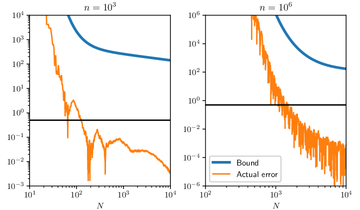
This brings us to the question of how (3) can be improved. The ingredients in the derivation of this bound are [3, Section 5.1]:
- •
The Weil bound .
- •
The bound for the number of divisors of .
- •
Bounding the sum of terms in (2) by a sum of absolute values of the terms.
The bound is not optimal. However, this bound is quite reasonable over the relevant non-asymptotic range of . If we could estimate by its average value , and show that the deviations from the average give a negligible contribution, we would get a constant around , which is much better but still rather impractical for computations.
It therefore seems that a useful error bound will require a much more involved analysis of cancellation in sums of Kloosterman sums. This is a well-studied problem [15], but it appears that all published results stronger than the Weil bound are asymptotic without explicit constants. We leave it as an open problem to prove sharp bounds for .
4. Hybrid algorithm
To get around the issues discussed in the previous section without sacrificing rigor, we make the following modification: instead of computing directly, we assume that is known modulo some integer . If we denote by the unique residue of with , we have . We can now compute using (2), stopping the summation when the bound for is just less than instead of . If we choose large enough, the truncation error is in the exponentially-large domain of the Bessel function (Lemma 3.2) where the available error bound works well.
For a general index , we can compute the residue of in using the power series (1). We can either compute a single power series over or choose a composite modulus, say , and compute the value for each in order to minimize memory usage. If is bounded, the memory usage will be , and the running time will be . This is not as good as the Petersson-Rademacher series would be if we had an optimal error bound, but it is better than computing using power series alone.
The optimal choice of will depend on the implementation-dependent relative speeds of the power series arithmetic and the numerical calculations for the Petersson-Rademacher series. In our experiments, we have obtained the best performance with slightly larger than for computing isolated values of . We get relatively uniform performance with anywhere between and while the running time increases sharply if is smaller than . If we want to compute a range of values of , it is more efficient to choose a larger , say word-size (or bigger, if sufficient memory is available), precomputing the residues once before using the Petersson-Rademacher series to determine the high bits for each coefficient of interest.
4.1. Special indices
When has special form, we can use known congruences for to determine a residue. For , we have
and there are also congruences modulo 11 and 13 [1, 12]. If is divisible by sufficiently many small primes, we can thus immediately construct a residue modulo an that is large enough (say ) to use the Petersson-Rademacher series. In that case, we do not need a power series evaluation, and the entire computation can be done using memory. Indeed, it is sufficient that is even, since this gives the comfortably large . If the obtained from congruences alone is too small, we can amend it with a power series computation modulo some larger prime.
5. Computations
We have implemented evaluation of using direct power series methods as well as the hybrid algorithm, using Flint [6] for power series and integer operations and Arb [10] for arbitrary-precision ball arithmetic. The following computations were performed on a laptop with 16 GB RAM and an Intel i5-4300U CPU.
| Digits in | PS () | PS2 () | NEW () | NEW () | ||
|---|---|---|---|---|---|---|
| 53 | 0.00011 | 0.00017 | 0.00033 | 0.00087 | ||
| 171 | 0.0068 | 0.015 | 0.0016 | 0.0041 | ||
| 543 | 0.33 | 0.96 | 0.0054 | 0.027 | ||
| 1722 | 15 | 48 | 0.025 | 0.22 | ||
| 5453 | 625 | 2169 | 0.13 | 2.5 | ||
| 17253 | (mem) | 0.83 | 32 | |||
| 54569 | 6.5 | 380 | ||||
| 172575 | (mem) | 60 | (mem) | |||
| 545743 | 636 |
5.1. Large values
As a benchmark (Table 1), we compute for various powers of ten as well as where is the first prime number after . Powers of ten are numbers of special form ( being divisible by ), meaning that the hybrid algorithm can use a congruence, skipping the power series evaluation. The subsequent prime number is of generic form (worst-case input) for the algorithm, forcing a power series evaluation to determine a residue.
For comparison purposes, we have implemented two versions of the power series algorithm to compute : the first using arithmetic in and the second using arithmetic modulo many small primes to conserve memory (which turns out to be roughly three times slower). The first power series implementation is roughly equivalent to the function j_invariant_qexp in SageMath [17].
We see that the hybrid algorithm is faster than the power series method already around . At , it is 250 times faster for the generic input (prime ) and 4800 times faster for the special-form input (power-of-ten ). The complexity of the hybrid algorithm is apparent in the running times.11 1 Arb does not presently use a quasi-optimal algorithm for the Bessel function at high precision, so if we were to continue the table beyond , the timings would likely get worse.
5.2. Prime values
The plethora of congruences satisfied by conspire to rule out being a prime number for small , but nothing suggests that this pattern must hold asymptotically. Indeed, while are all divisible by 2, 3 or 5, the smallest factor of is 353.
To search for prime values of , we used a single power series evaluation to compute several simultaneously modulo the primorial , which fits in a 64-bit word. We then selected the entries with and computed their full values using the hybrid algorithm with as precomputed input. Prime values of were then identified using a standard probabilistic primality test (trial factoring to rule out simple composites followed by the BPSW test).
To search up to , the initial power series calculation took three minutes. Filtering by left 28971 candidate to compute exactly (around 7 hours) and check for primality (around 45 hours).
| Digits in | ||
|---|---|---|
| 457871 | 3689 | |
| 685031 | 4513 | |
| 1029071 | 5532 | |
| 1101431 | 5723 | |
| 9407831 | 16734 | |
| 11769911 | 18718 | |
| 18437999 | 23429 |
Table 2 lists the first prime values of . At the time of writing, Jeremy Rouse reports having certified the primality of using ECPP. The remaining numbers are only confirmed as probable primes, but the BPSW test has no known counterexamples, and we anticipate that ECPP certificates can be generated with some months of computation.
Although primes seem to appear sparsely in the sequence (much more sparsely than for the partition function , for example), we speculate:
Conjecture 5.1.
There are infinitely many such that is prime.
With more memory and a large number of cores, the search could easily be extended further (at least to ). The method presented here could also be used to investigate other divisibility properties of the numbers .
6. Generalization
The methods discussed here are not specific to the -function. The Petersson-Rademacher series can be generalized to any modular function of weight 0 (see [3, Theorem 5.1]), and similar series can be constructed for the coefficients of a wide range of modular forms, or viewed combinatorially, for various partition-type sequences [16]. An interesting problem is to automate the efficient computation of such coefficients. Obtaining tight truncation bounds for Rademacher-type series seems difficult at the moment, but with the hybrid numerical-modular approach, more crude and generally applicable bounds can be used.
7. Source code
The author has made all source code and data behind this paper publicly available at https://github.com/fredrik-johansson/jfunction
References
- [1] Hans-Fredrik Aas. Congruences for the coefficients of the modular invariant . Mathematica Scandinavica, 14(2):185–192, 1964.
- [2] Harald Baier and Gunter Köhler. How to compute the coefficients of the elliptic modular function . Experimental Mathematics, 12(1):115–121, January 2003.
- [3] Nicolas Brisebarre and Georges Philibert. Effective lower and upper bounds for the Fourier coefficients of powers of the modular invariant . Journal of the Ramanujan Mathematical Society, 20(4):255–282, 2005.
- [4] John H. Conway and Simon P. Norton. Monstrous moonshine. Bulletin of the London Mathematical Society, 11(3):308–339, 1979.
- [5] David Feldman. Does the Fourier expansion of the -function have any prime coefficients? https://mathoverflow.net/q/377061, 2020.
- [6] William B. Hart. Fast library for number theory: An introduction. In Mathematical Software – ICMS 2010, pages 88–91. Springer Berlin Heidelberg, 2010.
- [7] OEIS Foundation Inc. The On-Line Encyclopedia of Integer Sequences. https://oeis.org/A000521, 2020.
- [8] Fredrik Johansson. Efficient implementation of the Hardy-Ramanujan-Rademacher formula. LMS Journal of Computation and Mathematics, 15:341–359, 2012.
- [9] Fredrik Johansson. Fast and rigorous computation of special functions to high precision. PhD thesis, RISC, Johannes Kepler University, Linz, 2014. http://fredrikj.net/thesis/.
- [10] Fredrik Johansson. Arb: Efficient arbitrary-precision midpoint-radius interval arithmetic. IEEE Transactions on Computers, 66(8):1281–1292, August 2017.
- [11] James Mc Laughlin and Scott Parsell. A Hardy-Ramanujan-Rademacher-type formula for -regular partitions. The Ramanujan Journal, 28(2):253–271, April 2012.
- [12] Morris Newman. Congruences for the coefficients of modular forms and for the coefficients of . Proceedings of the American Mathematical Society, 9(4):609, August 1958.
- [13] Hans Petersson. Über die Entwicklungskoeffizienten der automorphen Formen. Acta Mathematica, 58(1):169–215, 1932.
- [14] Hans Rademacher. The Fourier coefficients of the modular invariant . American Journal of Mathematics, 60(2):501, April 1938.
- [15] Peter Sarnak and Jacob Tsimerman. On Linnik and Selberg’s conjecture about sums of Kloosterman sums. In Algebra, Arithmetic, and Geometry, pages 619–635. Springer, 2009.
- [16] Andrew Sills. Towards an automation of the circle method. Gems in experimental mathematics, pages 321–338, 2010.
- [17] The Sage Developers. SageMath, the Sage Mathematics Software System (Version 9.0), 2020. https://www.sagemath.org.
- [18] Albert Leon Whiteman. A note on Kloosterman sums. Bulletin of the American Mathematical Society, 51(6):373–377, 1945.