Compact Objects in Entangled Relativity

First of all, we note as

$$D^{\alpha}_{\beta}=\frac{1}{\phi}(\nabla^{\alpha}\nabla_{\beta}-\delta^{\alpha}_{\beta}\square)\phi.$$

(9)

the dilaton energy-momentum tensor part in equation (3). The time-time component of the Einstein equations, leads to the following first order differential equation for $g_{rr}\equiv b$ metric component

$$\dfrac{\dot{b}}{b}=\dfrac{1-b}{r}+rb\left(\dfrac{\tilde{\kappa}\rho}{\sqrt{\phi}}-D^{0}_{0}\right),$$

(10)

where

$$D^{0}_{0}=\dfrac{1}{2b}\dfrac{\dot{\phi}}{\phi}\dfrac{\dot{a}}{a}+\dfrac{\tilde{\kappa}}{3\sqrt{\phi}}(\mathcal{L}_{m}-T).$$

(11)

One can formally integrate equation (10) for $b$, which leads to

$$b=\frac{1}{1-m\tilde{\kappa}/4\pi r},$$

(12)

where

$$m(r)\equiv\frac{4\pi}{\tilde{\kappa}}\int_{0}^{r}\mathrm{d}r\left(\frac{\rho}{\sqrt{\phi}}\tilde{\kappa}-\frac{1}{2b}\frac{\dot{\phi}}{\phi}\frac{\dot{a}}{a}-\frac{\tilde{\kappa}}{3\sqrt{\phi}}\left(\mathcal{L}_{m}-T\right)\right)r^{2}.$$

(13)

From (12), the ADM mass reads

$$\mathfrak{M}_{ADM}=\lim\limits_{r\rightarrow\infty}m(r),$$

(14)

and does not necessarily coincide with the star mass $m_{*}$ defined by

$$m_{*}=m(R_{*}),\hskip 5.69046pt\text{with }p(R_{*})=0.$$

(15)

Indeed, outside the star, matter energy density and pressure are negligible, so that they are set to zero and the relation between the ADM mass and the star mass reads

$$\mathfrak{M}_{ADM}=m_{*}-\frac{2\pi}{\tilde{\kappa}}\lim\limits_{r\rightarrow\infty}\int_{R_{*}}^{r}\mathrm{d}r\frac{r^{2}}{b}\frac{\dot{\phi}}{\phi}\frac{\dot{a}}{a}$$

(16)

On the other side, the r-r component of the Einstein equation yield a first order differential equation for $g_{tt}\equiv a$

$$\frac{\dot{a}}{a}=\frac{b}{r}\left(\frac{Pr^{2}\tilde{\kappa}}{\sqrt{\phi}}+1-\frac{1}{b}-\frac{2r}{b}\frac{\dot{\phi}}{\phi}\right)\left(1+\frac{r}{2}\frac{\dot{\phi}}{\phi}\right)^{-1}.$$

(17)

Following Wald Wald 1984, we compute the pressure using the conservation equation from the diffeomorphism invariance

$$\nabla_{\alpha}T_{\beta}^{\alpha}=\left(\delta_{\beta}^{\alpha}\mathcal{L}_{m}-T_{\beta}^{\alpha}\right)\partial_{\alpha}\log\sqrt{\phi}\equiv F_{\beta}$$

(18)

where the covariant derivative of a perfect fluid stress-energy tensor reads

	$\displaystyle\nabla_{\alpha}T_{\beta}^{\alpha}$	$\displaystyle=$	$\displaystyle\left(\delta_{\beta}^{\alpha}+u^{\alpha}u_{\beta}\right)\partial_{\alpha}P+(P+\rho)u^{\alpha}\nabla_{\alpha}u_{\beta}$		(19)
			$\displaystyle+u_{\beta}\left[u^{\alpha}\partial_{\alpha}\rho+(P+\rho)\nabla_{\alpha}u^{\alpha}\right].$

Projecting the last equation on $\partial_{r}$ and using $(\partial_{r})^{\mu}u_{\mu}=0$ brings up a derivative of the pressure with respect to the radius and we end up with

$$\dot{P}=-\frac{\dot{a}}{2a}(P+\rho)+\frac{\dot{\phi}}{2\phi}\left(\mathcal{L}_{m}-P\right).$$

(20)

The scalar-field equation reduces to

$$\ddot{\phi}=-\frac{\dot{\phi}}{2}\left[\frac{\dot{a}}{a}-\frac{\dot{b}}{b}+\frac{4}{r}\right]+\frac{\tilde{\kappa}\sqrt{\phi}}{3}b\left(T-\mathcal{L}_{m}\right).$$

(21)

At this point, the system can be fully inverted from $(a,b,\phi)$ to $(m,P,\phi)$. Indeed, $b$ has been expressed as a function of $m$ and differential equation for $a$ and $b$ are function of $(b,P,\phi)$. Then, we end up with the following system of first order differential equation

	$\displaystyle\dot{P}=-\dfrac{F_{1}}{2}(P+\rho)+\dfrac{\Psi}{2\phi}(\mathcal{L}_{m}-P)$		(22)
	$\displaystyle\dot{m}=4\pi r^{2}\left(\frac{\rho}{\sqrt{\phi}}-\frac{F_{3}}{\tilde{\kappa}}\right)$		(23)
	$\displaystyle\dot{\phi}=\Psi$		(24)
	$\displaystyle\dot{\Psi}=-\dfrac{\Psi}{2}\left[F_{1}-F_{2}+\dfrac{4}{r}\right]+\dfrac{\tilde{\kappa}\sqrt{\phi}}{3}b(T-\mathcal{L}_{m})$		(25)

with

	$\displaystyle F_{1}=\dfrac{b}{r}\left(\dfrac{Pr^{2}\tilde{\kappa}}{\sqrt{\phi}}+1-\dfrac{1}{b}-\dfrac{2r}{b}\dfrac{\Psi}{\phi}\right)\left(1+\dfrac{r}{2}\dfrac{\Psi}{\phi}\right)^{-1}$		(26)
	$\displaystyle F_{2}=\dfrac{1-b}{r}+rb\left(\dfrac{\tilde{\kappa}\rho}{\sqrt{\phi}}-F_{3}\right)$		(27)
	$\displaystyle F_{3}=\dfrac{1}{2b}\dfrac{\Psi}{\phi}F_{1}+\dfrac{\tilde{\kappa}}{3\sqrt{\phi}}(\mathcal{L}_{m}-T)$		(28)
	$\displaystyle b=\dfrac{1}{1-m\tilde{\kappa}/4\pi r}$		(29)

We assume a simple polytropic equation of state in this exploratory study, as the goal of this study is to see the broad behavior of compact object solutions in entangled relativity, compared to general relativity. Besides, the equations for matter fields are modified in entangled relativity due to the non-minimal coupling between geometry and matter—see Eq. (5). As a consequence, nuclear physics may be impacted at high density, which leads to many new open questions that are beyond the scope of this manuscript.

The equation of state that we shall consider reads

$$P=K\rho^{\gamma},$$

(30)

with $\gamma=5/3$ and $K=1.475\times 10^{-3}(fm^{3}/MeV)^{2/3}$ Schlögel et al. 2014.

We shall limit our investigations to solutions that have a sub-luminal speed of sound $v_{S}$ everywhere in the compact object. The condition implemented in our code reads

$$\frac{v_{S}}{c}\equiv\left(\frac{dP}{d\rho}\right)^{1/2}=\left(\gamma\frac{P}{\rho}\right)^{1/2}<1~\forall r\in~]0,R_{*}],$$

(31)

where $R_{*}$ is the radius of the compact object.

Now, one ought to know what is the value of the on-shell matter Lagrangian.¹¹ 1 By on-shell, here we mean the effective value that takes the Lagrangian when the matter field solutions are injected into its formal definition. Eventually, one may be able to derive it from first principles. However, the task is somewhat complex, given the additional complication that the matter field equations are modified with respect to general relativity, due to the non-minimal coupling between matter and geometry in entangled relativity—for instance, the modified Maxwell equation reads $\nabla_{\nu}\left(\sqrt{\phi}F^{\mu\nu}\right)=0$, where $F^{\mu\nu}$ is the usual electromagnetic tensor.

In what follows we will assume an effective perfect fluid description of matter fields, whose matter field density is conserved $\nabla_{\sigma}(\rho_{0}u^{\sigma})=0$—where $\rho_{0}$ is the rest-mass energy density—such that one can show that the matter Lagrangian reduces to $\mathcal{L}_{m}=-\rho$, where $\rho$ is the total energy density of the fluid Minazzoli and Harko 2012; Minazzoli 2013—see Appendix A. In that case, one can see in Eq. (4) that the scalar-field would only be sourced by pressure, such that this type of scalar-fields has been dubbed pressuron in Minazzoli and Hees 2014.

However, it has recently been argued that for generic solitons, the on-shell Lagrangian ought to reduce to the trace of the stress-energy tensor $\mathcal{L}_{m}=T$ Avelino and Azevedo 2018; *avelino:2018pd. If that argument held for compact objects such as neutron stars, one can see from Eq. (4) that the decoupling of the scalar-field would be total, such that one could expect to recover the results of general relativity. We checked that if we assume $\mathcal{L}_{m}=T$ instead of $\mathcal{L}_{m}=-\rho$, we indeed recover the TOV solutions of general relativity. ²² 2 Note that entangled relativity would nevertheless be different from general relativity for any matter field that do not satisfy $\mathcal{L}_{m}=T$, such as, for instance a pure magnetic field— which leads to $\mathcal{L}_{m}\propto B^{2}\neq T$ Thorsrud et al. 2012—or an homogeneous scalar field—which leads to $\mathcal{L}_{m}=P\neq T$ Turner 1983. In particular, one can expect the Higgs field to lead to a different behavior of the cosmic solution of entangled relativity close to the big bang, compared to general relativity.

Another interesting thing to keep in mind is that, since the on-shell Lagrangian $\mathcal{L}_{m}$ depends on the field solutions, one cannot a priori exclude the possibility that it could transition from, say, $\mathcal{L}_{m}=-\rho$ to $\mathcal{L}_{m}=T$, or $\mathcal{L}_{m}=T$ to $\mathcal{L}_{m}=P$, etc., after a phase transition of matter fields at some density inside the compact object. Studying this is beyond the scope of the present paper, as it would require to derive the behavior of matter fields from first principles; whereas we assume here an effective perfect fluid description. What is clear however, is that in the dust limit, one has $\mathcal{L}_{m}=-\rho=T$. Hence, $\mathcal{L}_{m}=P$ seems to be excluded, unless the aforementioned transition of phase can occur at high enough energy or pressure. But again, this is beyond the scope of the present manuscript.

We normalize the scalar field such that $\tilde{\kappa}/\sqrt{\phi_{L}}=8\pi G/c^{4}$, where $G$ is the measured value of the constant of Newton in the solar system, and $\phi_{L}$ the asymptotic value of the scalar field at a distance $r=L$ where the derivative of the gravitational potential becomes negligible, such that it matches the zeroth order of the post-Newtonian expansion of the theory in the weak-field regime of the solar system Minazzoli and Hees 2013. Note however that in practice, the effective value of $\phi_{L}$ can in principle take different values at different locations of the universe, which corresponds in effect to a constant of Newton that actually depends on the location. However, given the fact that the scalar field is not sourced by pressureless matter fields in the weak field regime Minazzoli and Hees 2013, one does not expect the two values to differ significantly in a dust³³ 3 Baryonic and cold dark matter. dominated environment such as our own galaxy.

Numerically, the choice $\tilde{\kappa}=\kappa$ has been made, so that the normalization of the scalar field reads $\phi_{\infty}\equiv\phi_{L}=1$. The goal is then to find the central value $\phi_{0}$ that leads to that normalization. In order to do so, one could run the simulation several times with different central values of the scalar field, until the one that corresponds to the desired normalization is reached. However, for the sake of computational speed, one could take the advantage of the following property: if $(\phi,\psi,m,P)(r)$ are solution of (22-25), then $(\alpha\phi,\psi,\alpha^{-1/4}m,\alpha P)(\alpha^{-1/4}r)$ are another solution $\forall\alpha$. If a simulation starts with a random initial value $\phi_{0}$ and lead to a star radius $\mathfrak{R}_{*}$, and an asymptotic scalar field value $\phi_{\infty}$, then, the radius with the appropriate units is $R_{*}=\phi_{\infty}^{1/4}\mathfrak{R}_{*}$, where the property has been used with $\alpha=\phi_{\infty}^{-1}$.

Because the dilaton field is sourced by pressure when $\mathcal{L}_{m}=-\rho$, and because the pressure increases with the density, one expects to have an increasing deviation from general relativity with the growth of the density. In the figures 1 and 2, one can see that this is broadly the case, although one should have a look at the metric in different cases in order to have a full picture of this. In particular, the denser the object, the more the metric deviates from the Schwarzschild metric outside the compact object—see Sec. IV.6. Also, one can see that, for central densities between 100 and 8200 $Mev/fm^{3}$, both the mass and the radius of the compact object are always higher in entangled relativity. The limit at 8200 $Mev/fm^{3}$ is set by the condition that the speed of sound in the compact object never exceeds the causality speed limit $c$.

One can see that, for a given central density, the mass $m_{*}$—defined in Eq. (15)—is always bigger in entangled relativity with respect to general relativity. The same is true for the ADM mass $\mathfrak{M}_{ADM}$—defined in Eq. (14)—, although the ADM mass is always smaller than the mass $m_{*}$, as one can see in Fig. 4. The difference between $m_{*}$ and $\mathfrak{M}_{ADM}$ simply comes from the infinite range contribution of the scalar-field to the mass—defined in Eq. (13).

At this stage, it would be tempting to argue that, as a consequence, entangled relativity may be a good candidate to explain the relatively high masses of neutron stars observed over the last decade Alsing et al. 2018, and which seem to lead to a tension between astrophysical observations and the union of general relativity and nuclear physics Biswas et al. 2020. However, this is way too premature given that one has to check first how the observables that are used to infer those masses from observations are actually affected in entangled relativity. For instance, one has to see how the Shapiro delay is modified in entangled relativity with respect to general relativity, and see how the inferred mass depends on the adjustment of the data in the new framework of entangled relativity. One has to note in particular that, unlike in general relativity, the mass of a compact object—defined in Eq. (13)—continues to change outside the compact object due to the contribution of the scalar-field. It continuously goes from $m_{*}$—defined in Eq. (15)—to $\mathfrak{M}_{ADM}$—defined in Eq. (14). This will affect observables that are sensitive to the metric outside the compact object—see Sec. IV.7.

Another interesting thing to point out is that, for a given central density, there is not a big difference in terms of radius between the predictions of general relativity and entangled relativity, as one can see in Fig. 2. On the other hand, for a given mass, the radius of high density (small radius) objects in entangled relativity are always smaller than in general relativity; whereas it is the opposite for low density (large radius) objects ⁴⁴ 4 resp. l.h.s. and r.h.s. of Fig. 3..

The scalar field grows monotonically from the center to infinity—where it reaches its normalized value $\phi_{\infty}=1$. In both the cases that lead to, e.g., $M=1.25M_{\odot}$—that is, the solutions with $400~MeV/fm^{3}$ and $4150~MeV/fm^{3}$ central densities—the scalar field derivative reaches a maximum toward roughly half the radius before monotonically decreasing to zero. Since matter physics depends on this derivative—see for instance Eq. (5)—it means that most of the effect of the scalar field happens inside the compact object. Nevertheless, the scalar field derivative is not null outside the compact object, such that one can expect entangled relativity to have a richier phenomenology with respect to general relativity—because of the scalar field’s behavior outside the compact object.

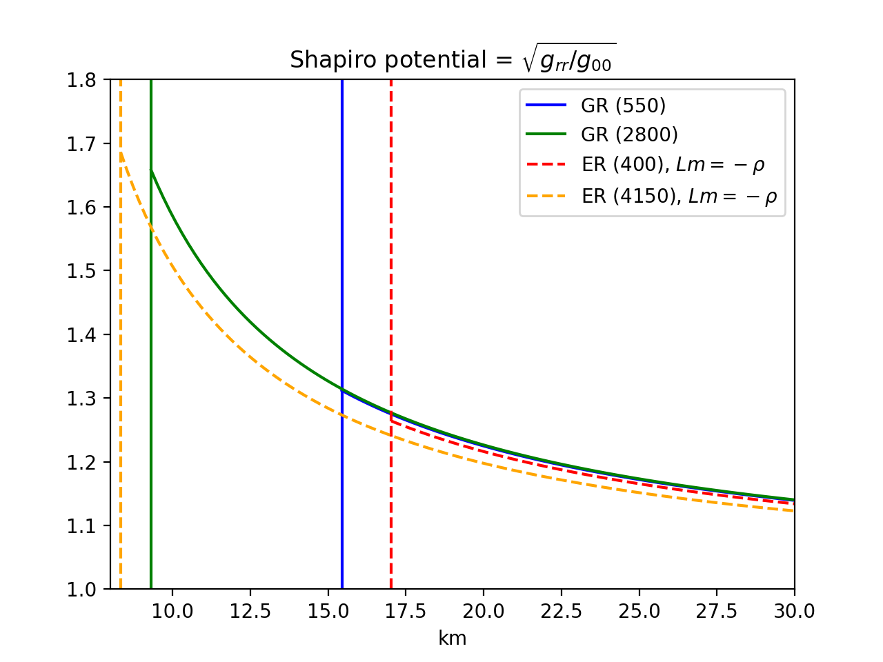
Most of the time, the mass of the compact object is degenerate with respect to the value of its central density, as one can see in Fig. 1. In general relativity, the specific value of the central density for two solutions with the same mass only plays a role with respect to the radius of the compact object, as Birkhoff’s theorem implies that the external metric ought to be the same for different solutions of an object of a given mass. However, Birkhoff’s theorem no longer holds in entangled relativity. Notably, unlike the case of general relativity, the scalar product between the time-time and space-space components of the metric outside a body is not a constant in entangled relativity. In Fig. 6, we show the product of the metric’s components $g_{00}g_{rr}$ of the two solutions of an object of mass $M=1.25M_{\odot}$ for each theory. In general relativity, the central density for this mass $M$ can either be around $550~MeV/fm^{3}$ or $2800~MeV/fm^{3}$, corresponding to a radius of 15.4 km or 9.3 km respectively; whereas in entangled relativity, it can either be around $400~MeV/fm^{3}$ or $4150~MeV/fm^{3}$, corresponding to a radius of 17.0 km or 8.3 km respectively.

As one can see, one has $g_{00}g_{rr}=$ cst outside the compact object in general relativity in each case, whereas it is no longer the case in entangled relativity. In particular, the denser the object, the more different is the metric’s components with respect to general relativity. It is the expected behavior, given that the scalar field is more sourced for denser objects.

Since the metric’s components deviate from the one of general relativity, one should expect the Shapiro delay to be modified accordingly. In particular, we shall expect that (what we shall call) the Shapiro potential—defined here as equal to $\sqrt{g_{rr}/g_{00}}$—should be modified with respect to general relativity. However, we see in Fig. 7 that the Shapiro potential remains qualitatively the same in entangled relativity.

The prediction of the mass and radius of neutron stars is not enough in order to test the theory for two reasons. First, those quantities depend significantly on the unknown equation of state of neutron stars. As a consequence, it may always be possible to tune the equation of state to recover the observed radius and mass. Second, the mass is not an observable, but is inferred from observables—such as the differential Shapiro time delay. Hence, one has to readjust the model parameters (such as the mass and the radius) from observations within the new framework before being able to say whether or not the theory explains the actual data well. For instance, regarding the Shapiro delay, because the metric outside the neutron star is not the Schwarzschild metric, the differential Shapiro delay does not follow the equation of general relativity that links the effect to the mass of the spherical compact object. Therefore, the mass of various neutron stars that have been inferred by measuring the differential Shapiro delay and assuming general relativity Demorest et al. 2010; Fonseca et al. 2016; Cromartie et al. 2020 are likely no longer the best fit for entangled relativity. Unfortunately, because the Birkhoff’s theorem is not valid in entangled relativity, the differential Shapiro delay is not uniquely defined with the mass of the source and the differential distance of the light-ray to the source. For instance, one can see in Fig. 6 that the outside metrics for two more or less dense compact objects with the same mass are not the same in entangled relativity—unlike what happens in general relativity. This may complicate the inversion from the observables to the model parameters in entangled relativity.

A potential way to test the theory would be to use X-ray pulse profiles from NASA’s Neutron star Interior Composition Explorer (NICER) Gendreau and Arzoumanian 2017, as it was recently proposed in order to probe strong-field effects in scalar-tensor theory Silva and Yunes 2019a; Silva and Yunes 2019b; Xu et al. 2020. In order to do so, one would have to extend the present work to the rotating case, as well as to consider more realistic equations of state. However, let us stress again that the matter field equations are modified in entangled relativity with respect to general relativity. This may induce yet another complication in such a study. Finally, let us note that unlike in the cases considered in Silva and Yunes 2019a; Silva and Yunes 2019b; Xu et al. 2020, the electromagnetic intensity is not conserved in entangled relativity due to the non-minimal coupling between the scalar degree of freedom and the electromagnetic field in the action Minazzoli and Hees 2014; *minazzoli:2014pl. This additional effect will have to be taken into account in order to correctly predict the variety of X-ray pulse profiles in entangled relativity.

Obviously, another way to test the theory would be through the observation of gravitational waves that have been emitted during the fusion of neutron stars Abbott et al. et al. 2017—although, again, the potential degeneracy with the unknown neutron star equation of state might limit the constraining power of such tests. This has yet to be explored.

References

- Ludwig et al. (2015) Hendrik Ludwig, Olivier Minazzoli, and Salvatore Capozziello, “Merging matter and geometry in the same Lagrangian,” Physics Letters B 751, 576–578 (2015), arXiv:1506.03278 [gr-qc] .
- Minazzoli (2018) Olivier Minazzoli, “Rethinking the link between matter and geometry,” Phys. Rev. D 98, 124020 (2018), arXiv:1811.05845 [gr-qc] .
- Minazzoli and Hees (2013) Olivier Minazzoli and Aurélien Hees, “Intrinsic Solar System decoupling of a scalar-tensor theory with a universal coupling between the scalar field and the matter Lagrangian,” Phys. Rev. D 88, 041504 (2013), arXiv:1308.2770 [gr-qc] .
- Minazzoli and Hees (2014) Olivier Minazzoli and Aurélien Hees, “Late-time cosmology of a scalar-tensor theory with a universal multiplicative coupling between the scalar field and the matter Lagrangian,” Phys. Rev. D 90, 023017 (2014), arXiv:1404.4266 [gr-qc] .
- Minazzoli (2014) Olivier Minazzoli, “On the cosmic convergence mechanism of the massless dilaton,” Physics Letters B 735, 119–121 (2014), arXiv:1312.4357 [gr-qc] .
- Minazzoli and Hees (2016) Olivier Minazzoli and Aurélien Hees, “Dilatons with intrinsic decouplings,” Phys. Rev. D 94, 064038 (2016), arXiv:1512.05232 [gr-qc] .
- (7) Olivier Minazzoli, “De Sitter space-times in Entangled Relativity,” in preparation .
- (8) Olivier Minazzoli and Edison Santos, “External Schwarzschild metric as a good approximation of spherical black hole solutions in Entangled Relativity,” in preparation .
- Wald (1984) R. M. Wald, General relativity (1984).
- (10) Code and script to compute all the figures, https://github.com/olivierrousselle/TOV-dilaton/tree/integration.
- Schlögel et al. (2014) Sandrine Schlögel, Massimiliano Rinaldi, François Staelens, and André Füzfa, “Particlelike solutions in modified gravity: The Higgs monopole,” Phys. Rev. D 90, 044056 (2014), arXiv:1405.5476 [gr-qc] .
- Minazzoli and Harko (2012) Olivier Minazzoli and Tiberiu Harko, “New derivation of the Lagrangian of a perfect fluid with a barotropic equation of state,” Phys. Rev. D 86, 087502 (2012), arXiv:1209.2754 [gr-qc] .
- Minazzoli (2013) Olivier Minazzoli, “Conservation laws in theories with universal gravity/matter coupling,” Phys. Rev. D 88, 027506 (2013), arXiv:1307.1590 [gr-qc] .
- Avelino and Azevedo (2018) P. P. Avelino and R. P. L. Azevedo, “Perfect fluid lagrangian and its cosmological implications in theories of gravity with nonminimally coupled matter fields,” Phys. Rev. D 97, 064018 (2018).
- Avelino and Sousa (2018) P. P. Avelino and L. Sousa, “Matter lagrangian of particles and fluids,” Phys. Rev. D 97, 064019 (2018).
- Thorsrud et al. (2012) Mikjel Thorsrud, David F. Mota, and Sigbjørn Hervik, “Cosmology of a scalar field coupled to matter and an isotropy-violating Maxwell field,” Journal of High Energy Physics 2012, 66 (2012), arXiv:1205.6261 [hep-th] .
- Turner (1983) Michael S. Turner, “Coherent scalar-field oscillations in an expanding universe,” Phys. Rev. D 28, 1243–1247 (1983).
- Alsing et al. (2018) Justin Alsing, Hector O. Silva, and Emanuele Berti, “Evidence for a maximum mass cut-off in the neutron star mass distribution and constraints on the equation of state,” MNRAS 478, 1377–1391 (2018), arXiv:1709.07889 [astro-ph.HE] .
- Biswas et al. (2020) Bhaskar Biswas, Prasanta Char, Rana Nandi, and Sukanta Bose, “Hint of a tension between Nuclear physics and Astrophysical observations,” arXiv e-prints , arXiv:2008.01582 (2020), arXiv:2008.01582 [astro-ph.HE] .
- Demorest et al. (2010) P. B. Demorest, T. Pennucci, S. M. Ransom, M. S. E. Roberts, and J. W. T. Hessels, “A two-solar-mass neutron star measured using Shapiro delay,” Nature 467, 1081–1083 (2010), arXiv:1010.5788 [astro-ph.HE] .
- Fonseca et al. (2016) Emmanuel Fonseca, Timothy T. Pennucci, Justin A. Ellis, Ingrid H. Stairs, David J. Nice, Scott M. Ransom, Paul B. Demorest, Zaven Arzoumanian, Kathryn Crowter, Timothy Dolch, Robert D. Ferdman, Marjorie E. Gonzalez, Glenn Jones, Megan L. Jones, Michael T. Lam, Lina Levin, Maura A. McLaughlin, Kevin Stovall, Joseph K. Swiggum, and Weiwei Zhu, “The NANOGrav Nine-year Data Set: Mass and Geometric Measurements of Binary Millisecond Pulsars,” ApJ 832, 167 (2016), arXiv:1603.00545 [astro-ph.HE] .
- Cromartie et al. (2020) H. T. Cromartie, E. Fonseca, S. M. Ransom, P. B. Demorest, Z. Arzoumanian, H. Blumer, P. R. Brook, M. E. DeCesar, T. Dolch, J. A. Ellis, R. D. Ferdman, E. C. Ferrara, N. Garver-Daniels, P. A. Gentile, M. L. Jones, M. T. Lam, D. R. Lorimer, R. S. Lynch, M. A. McLaughlin, C. Ng, D. J. Nice, T. T. Pennucci, R. Spiewak, I. H. Stairs, K. Stovall, J. K. Swiggum, and W. W. Zhu, “Relativistic Shapiro delay measurements of an extremely massive millisecond pulsar,” Nature Astronomy 4, 72–76 (2020), arXiv:1904.06759 [astro-ph.HE] .
- Gendreau and Arzoumanian (2017) Keith Gendreau and Zaven Arzoumanian, “Searching for a pulse,” Nature Astronomy 1, 895–895 (2017).
- Silva and Yunes (2019a) Hector O. Silva and Nicolás Yunes, “Neutron star pulse profiles in scalar-tensor theories of gravity,” Phys. Rev. D 99, 044034 (2019a), arXiv:1808.04391 [gr-qc] .
- Silva and Yunes (2019b) Hector O. Silva and Nicolás Yunes, “Neutron star pulse profile observations as extreme gravity probes,” Classical and Quantum Gravity 36, 17LT01 (2019b), arXiv:1902.10269 [gr-qc] .
- Xu et al. (2020) Rui Xu, Yong Gao, and Lijing Shao, “Strong-field effects in massive scalar-tensor gravity for slowly spinning neutron stars and application to x-ray pulsar pulse profiles,” Phys. Rev. D 102, 064057 (2020), arXiv:2007.10080 [gr-qc] .
- Abbott et al. et al. (2017) B. P. Abbott et al., LIGO Scientific Collaboration, and Virgo Collaboration, “GW170817: Observation of Gravitational Waves from a Binary Neutron Star Inspiral,” Phys. Rev. Lett. 119, 161101 (2017), arXiv:1710.05832 [gr-qc] .
Appendix A Perfect fluid Lagrangian and conservation of the rest-mass density
In this section, we slightly modify a demonstration that can already be found in Minazzoli 2013. Let us assume that the rest-mass density is not conserved, such that