Output Feedback Consensus for Networked Heterogeneous Nonlinear Negative-Imaginary Systems with Free Body Motion
Abstract
This paper provides a protocol to address the robust output feedback consensus problem for networked heterogeneous nonlinear negative-imaginary (NI) systems with free body dynamics. We extend the definition of nonlinear NI systems to allow for systems with free body motion. A new stability result is developed for the interconnection of a nonlinear NI system and a nonlinear output strictly negative-imaginary (OSNI) system. Also, a class of networked nonlinear OSNI controllers is proposed to achieve output feedback consensus for heterogeneous networked nonlinear NI systems. We show that in this control framework, the system outputs converge to the same limit trajectory. This consensus protocol is illustrated by a numerical example.
Index Terms:
nonlinear Negative-Imaginary systems, free body motion, heterogeneous systems, consensus, robust control.I INTRODUCTION
Negative-Imaginary (NI) systems theory was introduced by Lanzon and Petersen in [1] and [2] to address a robust control problem for flexible structures and has attracted much attention among control theory researchers (see [3, 4, 5, 6, 7, 8, 9]). Typical NI systems are systems with colocated force actuators and position sensors. Positive-Real (PR) systems theory [10] cannot be applied to the control of such systems in general. An NI system was initially defined in [1] to be a stable system with a frequency response satisfying for all . Examples of such systems arise in lightly damped structures [11, 12, 13] and nano-positioning systems [14, 15, 16, 17]. The stability of an NI system with transfer function matrix can be guaranteed by applying a strictly Negative-Imaginary (SNI) controller with transfer function matrix such that the DC gain condition is satisfied [1].
The definition of NI systems in [1, 2] was extended in [9] to include systems with poles in the closed left half of the complex plane except at the origin. The definition has been extended again in [18] to include systems with poles at the origin. Systems with free body motion such as single integrators and double integrators were included in this new definition and a new robust stability result for NI systems in [18]. The original definition of NI systems has also been recently extended to include nonlinear systems [19] and some stability results were established for nonlinear NI systems in [19] and [20]. However, systems with free body motion are excluded in the nonlinear NI definition in [19].
Cooperative control for multi-agent systems has been a highly active research area over the past two decades [21]. This control paradigm enables multiple systems to perform team missions and has been applied on autonomous vehicles including mobile robots, unmanned air vehicles (UAVs), autonomous underwater vehicles (AUVs) and other applications [22]. Consensus, that is convergence to an agreement through information sharing among agents, is one of the most important problems in the area of cooperative control [23]. Consensus algorithms were first studied for first-order dynamics (see [24, 25, 26], etc) and then extended to second-order systems (see [27, 28, 29, 30], etc).
As NI properties arise naturally in autonomous vehicles and a wide variety of other applications [31], consensus problems were investigated in [8] for heterogeneous NI systems. Using NI systems theory, the consensus algorithms in [8] only require outputs of the agents, and consensus is guaranteed if a simple DC gain condition is satisfied. The theoretical result presented in [8] has already been applied to real-world cooperative control problems (see [32, 33, 34, 35, 36]). However, this result is restricted to linear systems. Motivated by nonlinear NI systems theory, the result of [8] has been recently extended in [37], which provides a protocol that achieves output feedback consensus for networked heterogeneous nonlinear NI systems. However, [37] uses the definition of nonlinear NI systems from [19], which excludes systems with free body motion such as integrators.
In this work, we use an alternative definition for a class of nonlinear NI systems to include systems with free body motion. We obtain a stability result for the interconnection of a nonlinear NI system and a nonlinear output strictly negative-imaginary (OSNI) system (see also [38] and [39] for linear OSNI systems), where nonlinear OSNI systems are also redefined to allow direct feedthrough from the input to the output. Then we consider the output feedback consensus problem for multiple nonlinear NI systems with different state-space models. We aim to find a control protocol such that the difference between the outputs of any two agents connected in a network converges to zero. We model the communication between multiple nonlinear NI systems using an undirected connected graph, where the nonlinear NI plants and the nonlinear OSNI controllers correspond to the nodes and the edges of the graph, respectively. Each controller takes the difference between the outputs of the two plants connected to it as input and feeds back its output to the plants. This forms an augmented system whose stability is investigated in order to achieve output consensus for the nonlinear NI plants. We prove the networked nonlinear NI plants act as an augmented nonlinear NI system and the networked nonlinear OSNI controllers act as an augmented nonlinear OSNI system. Therefore, the entire networked control system can be regarded as the interconnection of a nonlinear NI system and a nonlinear OSNI system. Similarly to the stability result mentioned above, an extended stability result is established for the networked control system that guarantees output consensus. This shows that for networked heterogeneous nonlinear NI systems satisfying certain assumptions, output feedback consensus can be achieved by using suitable nonlinear OSNI controllers in the proposed control framework. The control framework is robust with respect to bounded perturbations in the system models for both the nonlinear NI plants and the nonlinear OSNI controllers.
This paper contributes an output feedback consensus protocol for networked heterogeneous nonlinear NI systems with free body motion. This work differs from the related previous results in the following aspects: [19] defines nonlinear NI systems but does not allow for systems with free body motion while this work does; [20] only considers consensus for agents with the same model while this work allows agents to have different state-space models; [20] and [37] only deal with consensus problems for nonlinear NI systems without free body motion while this restriction is lifted in this work. This work can also be regarded as an extension of the papers [18] and [8] to nonlinear systems.
Notation: The notation in this paper is standard. and denote the fields of real and complex numbers, respectively. and denote the spaces of real and complex matrices of dimension , respectively. and denote the transpose and complex conjugate transpose of a matrix , respectively. denotes the maximum eigenvalue of a matrix with only real eigenvalues. denotes the Kronecker product of matrices and . denotes a constant value for a given vector or scalar signal. denotes the Euclidean norm of a vector. is the identity matrix. For a nonlinear dynamical system with input and output , describes its input-output relationship. represents a diagonal matrix with the values on its diagonal.
Graph Theory Preliminaries: , where and , describes an undirected graph with nodes and edges. The corresponding symmetric adjacency matrix is defined so that , and , if and otherwise. A sequence of unrepeated edges in that joins a sequence of nodes in defines a path. An undirected graph is connected if there is a path between every pair of nodes. Given an undirected graph , a corresponding directed graph can be obtained by defining a direction for each edge of . The incidence matrix of a directed graph is defined so that the elements in are given by
In this paper, the initial and terminal vertices of an edge in a directed graph can both send information to each other via the corresponding controller. For an undirected graph , the choice of a corresponding directed graph is not unique. However, the Laplacian matrix of has the following relationship with the incidence matrix of any directed graph corresponding to : .
II AN INITIAL STABILITY RESULT
In this section, new definitions of nonlinear NI and nonlinear OSNI systems are provided and a new stability result is established for the interconnection of a single nonlinear NI system and a single nonlinear OSNI system. The new stability result is applicable to nonlinear NI systems with free body motion, which are excluded in the previous stability result given in [20].
Consider the following general nonlinear system:
| (1) | ||||
| (2) |
where is the state, is the input, and is the output, is a Lipschitz continuous function, is a class function and is a symmetric matrix; i.e., .
Definition 1
In contrast to Definition 3 in [19], which excludes linear NI systems with poles at the origin, Definition 1 now includes all linear NI systems satisfying the definition given in [18] by allowing the storage function of the system to be positive semidefinite instead of positive definite.
Definition 2
The system (1), (2) is said to be a nonlinear output strictly negative-imaginary (OSNI) system if there exists a positive semidefinite storage function of class and a scalar such that
| (5) |
for all , where is as defined in (4). In this case, we also say that system (1), (2) is nonlinear OSNI with degree of output strictness .
In this paper, nonlinear OSNI systems defined as in Definition 2 are applied as controllers to achieve the robust output feedback consensus for networked heterogeneous nonlinear NI systems defined as in Definition 1. First, we provide a stability result for a single feedback interconnection of nonlinear NI systems.
Consider a multiple-input multiple-output (MIMO) nonlinear NI system with the following state-space model:
| (6) | ||||
| (7) |
where is the state, is the input, and is the output, is a Lipschitz continuous function and is a class function.
For the system with the state-space model (6), (7), we suppose the following assumption is satisfied.
Assumption I: When the system is in steady state; i.e., , and , we have .
For nonlinear NI systems, Assumption I corresponds to the property of linear NI systems stated in Lemma 2 in [1].
Consider a MIMO nonlinear OSNI system with the following state-space model:
| (8) | ||||
| (9) |
where is the state, is the input, and is the output, is a Lipschitz continuous function, is a class function and is a symmetric matrix; i.e., .
For the system with the state-space model (8), (9), we suppose that the following assumption is satisfied.
Assumption II: When the system is in steady state; i.e., , and , we have with .
It might be observed that as nonlinear OSNI systems belong to a subclass of nonlinear NI systems, Assumption II seems to have a conflicting relationship with Assumption I. In fact, Assumption II can be satisfied because of the term in the output equation (9) and it corresponds to the inequality (61) for linear NI systems in [18].
In addition, both of the systems and are assumed to satisfy the following assumptions. For the system with input , state and output described by the state-space model (6), (7) and the system with input , state and the auxiliary output described by the state-space model (8), (9), we suppose for and , the following conditions are satisfied.
Assumption III: Over any time interval where , remains constant if and only if remains constant; i.e., . Moreover, .
Assumption IV: Over any time interval where , remains constant only if remains constant; i.e., . Moreover, .
In the case of linear systems, Assumption III corresponds to observability and Assumption IV corresponds to the matrix in the realisation of the linear system having full column rank.

Theorem 1
Consider the closed-loop positive feedback interconnection of the system with state-space model (6), (7) and with state-space model (8), (9), as shown in Fig. 1. Suppose that Assumptions I-IV are satisfied, and the storage function, defined as
| (10) |
is positive definite, where and are positive semidefinite storage functions that satisfy (3) for the system and (5) for the system , respectively. Then, the closed-loop interconnection of the systems and is asymptotically stable.
Proof:
According to the nonlinear NI property (3) for the system , the nonlinear OSNI property (5) for the system and the system setting and in Fig. 1, we have
| (11) |
and
| (12) |
where the above equalities also use (7) and (9). We obtain the time derivative of the storage function in (10) using (11) and (12):
| (13) |
From this it follows that is only possible when . Hence, can remain zero only if remains zero; i.e., . According to Assumptions III and IV, . Hence, the system is in steady-state. According to the system setting in Fig. 1, . Hence, using Assumptions III and IV, . Thus, the system is also in steady-state. Then, according to Assumption II, we have
If , then . According to Assumptions III and IV, and the system setting in Fig. 1, . Hence, in this case, the system is in equilibrium. Otherwise, if , we have
| (14) |
Also, according to Assumption I, we have
| (15) |
According to the system setting in Fig. 1, we have and . Hence, (15) can be rewritten as
which contradicts (14). Thus, we can conclude that cannot remain zero unless . Thus, according to LaSalle’s invariance principle, will keep decreasing until . Hence, the equilibrium at of the closed-loop interconnection is asymptotically stable. ∎
III OUTPUT FEEDBACK CONSENSUS
Consider heterogeneous nonlinear plants described as
| (16) | ||||
| (17) |
where is the state, is the input, and is the output, are Lipschitz continuous functions and are class functions. These systems operate independently in parallel and each of them has its own input and output , (), which is shown in Fig. 2. The subscript “” indicates that this system will play the role of a plant in what follows. We combine the inputs and outputs respectively as the vectors and , respectively.

Let us consider the networked plants connected according to the graph network topology as shown in Fig. 3, where is the incidence matrix of a directed graph that represents the communication links between the heterogeneous nonlinear NI plants.

For the system shown in Fig. 3, we have the following lemma:
Lemma 1
If the plants are nonlinear NI systems for all , then the networked plant is also a nonlinear NI system.
Proof:
According to Definition 1, each nonlinear NI system () must have a corresponding positive semidefinite storage function such that , where is the state of the system . We define the storage function for the system as , which is positive semidefinite. Then
| (18) |
Let and denote the input and output of the system , respectively. According to the system setting in Fig. 3, we have
Therefore, we have
| (19) |
According to (18) and (19), we obtain the nonlinear NI inequality for the system :
| (20) |
Therefore, is a nonlinear NI system. ∎
Now we give a definition of output feedback consensus for a network of systems as shown in Fig. 2.
Definition 3
A distributed output feedback control law achieves output feedback consensus for a network of systems if as , .
Consider a series of heterogeneous nonlinear OSNI controllers applied at the edges in the network. The OSNI controllers have the following state-space models:
| (21) | ||||
| (22) |
where is the state, is the input, and is the output, are Lipschitz continuous functions, are class functions and are symmetric matrices. These systems operate independently in parallel and each of them has its own input and output , , which is shown in Fig. 4. The subscript “” indicates that this system will play the role of a controller in what follows. We combine the inputs and outputs respectively as the vectors and , where
| (23) |
and
| (24) |
Lemma 2
If the controllers are nonlinear OSNI systems for all , then the networked controller is also a nonlinear OSNI system.
Proof:
For every nonlinear OSNI system , we have a positive semidefinite storage function and a constant such that
| (25) |
where and is the level of output strictness of the system . For the system , we define its storage function as the sum of the storage functions of all the networked controllers; i.e.,, which is positive semidefinite. The time derivative of is:
| (26) |
where . Hence, the system satisfies the definition of a nonlinear OSNI system and quantifies a level of output strictness of the system. This completes the proof. ∎
Now consider the closed-loop positive feedback interconnection of the networked plants shown in Fig. 3 and the networked controllers shown in Fig. 4, which is depicted in Fig. 5. In this paper, robust output consensus of heterogeneous nonlinear NI plants is achieved by constructing a control system with the block diagram shown in Fig. 5 and choosing suitable controllers that satisfy certain conditions. Detailed description of the control framework in Fig. 5 can be found in [37], which uses a similar control framework.

As is shown in Fig. 5, the control input for the networked plant is
| (27) |
where is the incidence matrix of the directed graph that represents the communication links between the heterogeneous nonlinear NI plants. Equivalently, the distributed control protocol for the plant is defined by the equations
| (28) | ||||
| (29) | ||||
| (30) |
where and are the -th and -th elements in the -th row of the incidence matrix , respectively. Here, represents the difference between the outputs of the two plants connected by the edge .
Before we present the main result, let us make another assumption. For the system with input and output , we suppose the following assumption is satisfied.
Assumption V: Given a constant input to the system , if its output is also constant; i.e., , then and satisfy .
In fact, Assumption I implies Assumption V in the case that all the plants are in steady state. This is because when all the plants satisfy Assumption I and are in steady state, we have and according to the system setting in Fig. 5 we have similarly to (19). Hence . However, Assumption V is assumed for the networked plants in the following theorem instead of assuming Assumption I for each individual plant because Assumption V also allows for the situation in which the input and output of the system are constant, but the individual plants are not all in steady state. This situation is possible because the matrix takes the difference between the outputs of the plants. Under constant inputs, if the plants oscillate with a constant difference between their outputs, then this situation is allowed under Assumption V.
Theorem 2
Consider an undirected connected graph that models the communication links for a network of heterogeneous nonlinear NI systems as shown in Fig. 2, and any directed graph corresponding to with the incidence matrix . Also, consider the heterogeneous nonlinear OSNI control laws for all of the edges. Suppose Assumptions III and IV are satisfied for the plants , Assumptions II, III and IV are satisfied for the controllers (with for the controller in Assumption II) and Assumption V is satisfied by the system . Also, suppose the storage function, defined as
is positive definite, where and are positive semidefinite storage functions that satisfy (20) for the system and (26) for the system , respectively. Here, is the output of the system . and are terms in the output of the system and are defined in (23) and (24). Then robust output feedback consensus can be achieved via the protocol (27), or equivalently (28)-(30) in a distributed manner for each plant , as shown in Fig. 5.
Proof:
According to (20), (26) and the system setting and shown in Fig. 5, we have
| (31) |
and
| (32) |
According to (31), (32) and the symmetry of in (24), the time derivative of the storage function satisfies the following inequality:
| (33) |
Hence, the closed-loop system is at least Lyapunov stable. Moreover, can hold only if . In other words, can remain zero only if remains zero for all . According to Assumptions III and IV, . Hence, is in steady-state for all . We have and . According to the system setting in Fig. 5 that and , we also have and . According to Assumption V, we have
| (34) |
According to Assumption II, we have
where . In the case that , we have
| (35) |
which contradicts (34) because . In the case that , all connected plants have the difference between their system outputs being zero. Hence, output consensus has already been achieved. Otherwise, cannot remain zero. According to LaSalle’s invariance principle, will keep decreasing until either or . Thus, output consensus is achieved in both cases. This completes the proof. ∎
IV ILLUSTRATIVE EXAMPLE

Consider four nonlinear NI plants at the vertices of the graph in Fig. 6. We choose directions of the edges as , , and . Then the incidence matrix of the directed graph corresponding to is
The plants are nonlinear single integrators which have the following state-space models:
where , , and are constant coefficients. The storage functions for these four plants are all . The states , , and of these four plants have initial values , , and , respectively. We aim to synchronise the outputs of these four plants to the same limit trajectory by using nonlinear OSNI controllers at the edges of the graph in Fig.6.
where and are constant coefficients. , , , ; , , and , respectively.
The storage functions of Controllers , , and are , , and , respectively.
The networked plant system in this example is given by the equations:
The storage function of the closed-loop system provided by Theorem 2 takes the form
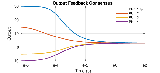
which is positive definite. Assumptions II-V in Sections II and III are satisfied. Output feedback consensus is achieved, as shown in Fig. 7. Because of the cubic nonlinearity in the plants and the controllers, their outputs have different rates of convergence in the domains where the states are far and close to the limit values. Therefore, a log scale is used for the time axis in the plot shown in Fig. 7.
V CONCLUSION
This paper provides a control framework to achieve robust output feedback consensus for networked heterogeneous nonlinear NI systems including systems with free body motion, using nonlinear OSNI controllers. New definitions for nonlinear NI systems and nonlinear OSNI systems are given and a stability result is established for the simple feedback interconnection of a nonlinear NI plant and a nonlinear OSNI controller. A networked control framework is then considered by modelling the communication topology between systems as a connected graph, where the plants are nodes and the controllers are edges. The network of nonlinear NI plants and the network of OSNI controllers are proved to be a nonlinear NI system and a nonlinear OSNI system, respectively. Under reasonable assumptions, output feedback consensus is established for the networked heterogeneous nonlinear NI systems, and the result is robust against variations in the system models of both the plants and controllers provided that the relevant nonlinear NI and nonlinear OSNI properties are preserved. Finally, an example is given to demonstrate the proposed result on a consensus problem to which earlier results are not applicable.
References
- [1] A. Lanzon and I. R. Petersen, “Stability robustness of a feedback interconnection of systems with negative imaginary frequency response,” IEEE Transactions on Automatic Control, vol. 53, no. 4, pp. 1042–1046, 2008.
- [2] I. R. Petersen and A. Lanzon, “Feedback control of negative-imaginary systems,” IEEE Control Systems Magazine, vol. 30, no. 5, pp. 54–72, 2010.
- [3] B. Bhikkaji, S. R. Moheimani, and I. R. Petersen, “A negative imaginary approach to modeling and control of a collocated structure,” IEEE/ASME Transactions on Mechatronics, vol. 17, no. 4, pp. 717–727, 2011.
- [4] J. Xiong, I. R. Petersen, and A. Lanzon, “On lossless negative imaginary systems,” in 2009 7th Asian Control Conference. IEEE, 2009, pp. 824–829.
- [5] Z. Song, A. Lanzon, S. Patra, and I. R. Petersen, “A negative-imaginary lemma without minimality assumptions and robust state-feedback synthesis for uncertain negative-imaginary systems,” Systems & Control Letters, vol. 61, no. 12, pp. 1269–1276, 2012.
- [6] J. Xiong, I. R. Petersen, and A. Lanzon, “Finite frequency negative imaginary systems,” IEEE Transactions on Automatic Control, vol. 57, no. 11, pp. 2917–2922, 2012.
- [7] Z. Song, A. Lanzon, S. Patra, and I. R. Petersen, “Robust performance analysis for uncertain negative-imaginary systems,” International Journal of Robust and Nonlinear Control, vol. 22, no. 3, pp. 262–281, 2012.
- [8] J. Wang, A. Lanzon, and I. R. Petersen, “Robust cooperative control of multiple heterogeneous negative-imaginary systems,” Automatica, vol. 61, pp. 64–72, 2015.
- [9] J. Xiong, I. R. Petersen, and A. Lanzon, “A negative imaginary lemma and the stability of interconnections of linear negative imaginary systems,” IEEE Transactions on Automatic Control, vol. 55, no. 10, pp. 2342–2347, 2010.
- [10] B. Brogliato, R. Lozano, B. Maschke, and O. Egeland, “Dissipative systems analysis and control,” Theory and Applications, vol. 2, 2007.
- [11] B. Bhikkaji and S. Moheimani, “Fast scanning using piezoelectric tube nanopositioners: A negative imaginary approach,” in 2009 IEEE/ASME International Conference on Advanced Intelligent Mechatronics. IEEE, 2009, pp. 274–279.
- [12] J. Fanson and T. K. Caughey, “Positive position feedback control for large space structures,” AIAA journal, vol. 28, no. 4, pp. 717–724, 1990.
- [13] C. Cai and G. Hagen, “Stability analysis for a string of coupled stable subsystems with negative imaginary frequency response,” IEEE Transactions on Automatic Control, vol. 55, no. 8, pp. 1958–1963, 2010.
- [14] J. van Hulzen, G. Schitter, P. Van den Hof, and J. Van Eijk, “Modal actuation for high bandwidth nano-positioning,” in Proceedings of the 2010 American Control Conference. IEEE, 2010, pp. 6525–6530.
- [15] S. Devasia, E. Eleftheriou, and S. R. Moheimani, “A survey of control issues in nanopositioning,” IEEE Transactions on Control Systems Technology, vol. 15, no. 5, pp. 802–823, 2007.
- [16] A. Sebastian and S. M. Salapaka, “Design methodologies for robust nano-positioning,” IEEE Transactions on Control Systems Technology, vol. 13, no. 6, pp. 868–876, 2005.
- [17] J. Dong, S. M. Salapaka, and P. M. Ferreira, “Robust MIMO control of a parallel kinematics nano-positioner for high resolution high bandwidth tracking and repetitive tasks,” in 2007 46th IEEE Conference on Decision and Control. IEEE, 2007, pp. 4495–4500.
- [18] M. A. Mabrok, A. G. Kallapur, I. R. Petersen, and A. Lanzon, “Generalizing negative imaginary systems theory to include free body dynamics: Control of highly resonant structures with free body motion,” IEEE Transactions on Automatic Control, vol. 59, no. 10, pp. 2692–2707, 2014.
- [19] A. G. Ghallab, M. A. Mabrok, and I. R. Petersen, “Extending negative imaginary systems theory to nonlinear systems,” in 2018 IEEE Conference on Decision and Control (CDC). IEEE, 2018, pp. 2348–2353.
- [20] K. Shi, I. Vladimirov, and I. Petersen, “Robust output feedback consensus for networked identical nonlinear negative-imaginary systems,” To appear in the 24th International Symposium on Mathematical Theory of Networks and Systems, arXiv:2005.11492, 2020.
- [21] R. M. Murray, “Recent research in cooperative control of multivehicle systems,” 2007.
- [22] W. Ren, R. W. Beard, and E. M. Atkins, “A survey of consensus problems in multi-agent coordination,” in Proceedings of the 2005, American Control Conference, 2005. IEEE, 2005, pp. 1859–1864.
- [23] W. Ren, “Consensus strategies for cooperative control of vehicle formations,” IET Control Theory & Applications, vol. 1, no. 2, pp. 505–512, 2007.
- [24] A. Jadbabaie, J. Lin, and A. S. Morse, “Coordination of groups of mobile autonomous agents using nearest neighbor rules,” IEEE Transactions on automatic control, vol. 48, no. 6, pp. 988–1001, 2003.
- [25] R. Olfati-Saber and R. M. Murray, “Consensus problems in networks of agents with switching topology and time-delays,” IEEE Transactions on automatic control, vol. 49, no. 9, pp. 1520–1533, 2004.
- [26] L. Moreau, “Stability of multiagent systems with time-dependent communication links,” IEEE Transactions on automatic control, vol. 50, no. 2, pp. 169–182, 2005.
- [27] H. G. Tanner, A. Jadbabaie, and G. J. Pappas, “Stable flocking of mobile agents, part i: Fixed topology,” in 42nd IEEE International Conference on Decision and Control (IEEE Cat. No. 03CH37475), vol. 2. IEEE, 2003, pp. 2010–2015.
- [28] R. O. Saber and R. M. Murray, “Flocking with obstacle avoidance: Cooperation with limited communication in mobile networks,” in 42nd IEEE International Conference on Decision and Control (IEEE Cat. No. 03CH37475), vol. 2. IEEE, 2003, pp. 2022–2028.
- [29] W. Yu, W. Ren, W. X. Zheng, G. Chen, and J. Lü, “Distributed control gains design for consensus in multi-agent systems with second-order nonlinear dynamics,” Automatica, vol. 49, no. 7, pp. 2107–2115, 2013.
- [30] H. Su, G. Chen, X. Wang, and Z. Lin, “Adaptive second-order consensus of networked mobile agents with nonlinear dynamics,” Automatica, vol. 47, no. 2, pp. 368–375, 2011.
- [31] I. R. Petersen, “Negative imaginary systems theory and applications,” Annual Reviews in Control, vol. 42, pp. 309–318, 2016.
- [32] V. P. Tran, M. Garratt, and I. R. Petersen, “Formation control of multi-uavs using negative-imaginary systems theory,” in 2017 11th Asian Control Conference (ASCC). IEEE, 2017, pp. 2031–2036.
- [33] Y. Qi, J. Wang, Q. Jia, and J. Shan, “Cooperative assembling using multiple robotic manipulators,” in 2016 35th Chinese Control Conference (CCC). IEEE, 2016, pp. 7973–7978.
- [34] J. Hu, P. Bhowmick, and A. Lanzon, “Distributed adaptive time-varying group formation tracking for multiagent systems with multiple leaders on directed graphs,” IEEE Transactions on Control of Network Systems, vol. 7, no. 1, pp. 140–150, 2019.
- [35] J. Peng, J. Wang, and J. Shan, “Robust cooperative tracking of multiple p-order power integrators,” in 2016 Chinese Control and Decision Conference (CCDC). IEEE, 2016, pp. 951–956.
- [36] O. Skeik, J. Hu, F. Arvin, and A. Lanzon, “Cooperative control of integrator negative imaginary systems with application to rendezvous multiple mobile robots,” in 2019 12th International Workshop on Robot Motion and Control (RoMoCo). IEEE, 2019, pp. 15–20.
- [37] K. Shi, I. G. Vladimirov, and I. R. Petersen, “Robust output feedback consensus for networked heterogeneous nonlinear negative-imaginary systems,” in 2020 Australian and New Zealand Control Conference (ANZCC), 2020, pp. 214–219.
- [38] P. Bhowmick and S. Patra, “On LTI output strictly negative-imaginary systems,” Systems & Control Letters, vol. 100, pp. 32–42, 2017.
- [39] P. Bhowmick and A. Lanzon, “Output strictly negative imaginary systems and its connections to dissipativity theory,” in 2019 IEEE 58th Conference on Decision and Control (CDC). IEEE, 2019, pp. 6754–6759.