Sideband transitions in a two-mode Josephson circuit driven beyond the rotating wave approximation
Abstract
Driving quantum systems periodically in time plays an essential role in the coherent control of quantum states. The rotating wave approximation (RWA) is a good approximation technique for weak and nearly-resonance driven fields. However, these experiments sometimes require large detuning and strong driving fields, for which the RWA may not hold. In this work, we experimentally, numerically, and analytically explore strongly driven two-mode Josephson circuits in the regime of strong driving and large detuning. Specifically, we investigate beam-splitter and two-mode squeezing interaction between the two modes induced by driving a two-photon sideband transition. Using numerical simulations, we observe that the RWA is unable to correctly capture the amplitude of the sideband transition rates. We verify this finding using an analytical model that is based on perturbative corrections. We find that the breakdown of the RWA in the regime studied does not lead to qualitatively different dynamics, but gives the same results as the RWA theory at higher drive strengths, enhancing the coupling rates compared to what one would predict. This is an interesting consequence compared to the carrier transition case, where the breakdown of the RWA results in qualitatively different time evolution of the quantum state. Our work provides an insight into the behavior of time-periodically driven systems beyond the RWA. We also provide a robust theoretical framework for including these findings in the calculation and calibration of quantum protocols in circuit quantum electrodynamics.
I Introduction
Time-periodic driving is a prominent technique for the coherent control of quantum dynamical processes. However, exactly solving the quantum dynamics of the system with time-varying Hamiltonian is particularly difficult Bloch-PR-1940; Giscard-PRR-2020. As long as the drive is weak enough and nearly resonant with the quantum state transition of a target observable, then the rotating wave approximation (RWA) may provide a good estimate of the dynamics RWA; note. It is, however, necessary to understand the physics of quantum systems beyond the RWA from both from a fundamental and a practical perspective. In the realm of faithful quantum information processing (QIP), the need for fast gates to suppress quantum errors requires drive strengths that could exceed those that are valid for the RWA. Motivated by this problem, theoretical effort has been directed to understand quantum driven systems beyond the RWA Bloch-PR-1940; Giscard-PRR-2020, along with many experimental works that have used strong driving across many different physical systems. Andrews-JPB-1975; Fuchs-Science-2009; Tuorila-PRL-2015; Deng-PRL-2015; Laucht-PRB-2016; Pietik-PRB-2016; Sie-Science-2017; Koski-PRL-2018. Although the previous studies have explored driven systems beyond the RWA, they focus on a single driven mode and do not address the coupling of different degrees of freedom (e.g., the use of driving fields to induce sideband transitions between modes).
Sideband transitions ubiquitously appear in a variety of physical systems Leek-PRB-2009; Leek-PRL-2010; Leghtas-Science; Mundhada-PRAppl-2019; Teufel-Nature-2011; Schliesser-NPhys-2008; Monroe-PRL-1995; Hennrichh-PRL-2000; Fedorov-PRA. Driving systems with appropriately chosen frequencies can yield engineered interactions among different degrees of freedoms. To engineer a specific interaction, it is important to accurately estimate the transition rates. In many cases the driving parameters for sideband transitions typically satisfy the requirements of the RWA, such as trapped ions, cavity-optomechanics, and Raman transitions Teufel-Nature-2011; Schliesser-NPhys-2008; Monroe-PRL-1995; Hennrichh-PRL-2000. However, this is not always the case for the circuit quantum elecrodynamics (cQED) platform, one of the most promising QIP platforms in recent years, where a strong and far off resonant driving beyond the RWA is sometimes required BANN-PRA. Nonetheless, current approaches to quantitative analysis still rely on the application of the RWA. When the sideband driving frequencies are far off-resonant from the transition frequencies of the system, in which the conditions for the application of the RWA should not hold, we may not currently be possible to make reliable predictions of the transition rates.
In this paper, we study the sideband transition rates in a two-mode Josephson circuit that is induced by strong external time-periodical driving. The circuit comprises a transmon Koch-PRA-2007 that is dispersively coupled to a resonator mode. Specifically, we study beam splitter (BS) and two-mode squeezing (TMS) interactions between each mode, which are the simplest forms of sideband transitions in these two-mode systems. For our device, the required driving parameters are close to (TMS coupling), or far beyond (BS coupling) the RWA regime. We confirm a simple relationship between the transition rates and frequency shifts, which explains the data in both regimes.
We perform numerical simulations to support our findings. We also derive an analytical perturbation expansion that goes beyond the RWA, which is validated by our numerical results. Our findings indicate that although the RWA is clearly violated, and significantly underestimates the mode frequency shifts and the sideband transition rates for a known driving strength, the breakdown of the RWA does not result in qualitatively different behaviour but instead its effects in our measurements can be reproduced by the RWA theory using a larger drive field. Although the confirmation of a breakdown of the RWA is only possible to observe experimentally in an accurate independent calibration of the drive field, our results show the importance of including counter-rotating terms for accurate calculations of the sideband transition rates.
II Theoretical description
We derive an analytical expression taking a similar approach in Reagor-thesis; Leghtas-Science but breaking the RWA. The total Hamiltonian on the lab frame is given by,
| (1) |
Here, and are the resonant frequencies of each mode. and are the mode destruction operators of the transmon and the resonator modes, respectively. is a Duffing nonlinearity of the transmon mode. is a transverse coupling between the transmon mode and the resonator mode. In addition to , there is the driving Hamiltonian , where and are the driving amplitude and frequency, respectively. The total Hamiltonian is then given by .
It is often useful to rewrite this Hamiltonian in the normal mode basis (the normal mode annihilation operators are and ):
| (2) |
With typical circuit QED parameters, is approximately the same as . is the inherited Duffing nonlinearity to the resonator mode by the coupling . In the dispersive coupling regime (), in can be approximated by Leghtas-Science; Gely-PRA-2018. Then, the driving Hamiltonian can be approximated to be .
The total Hamiltonian in the normal mode basis is then given by . This can be perturbatively diagonalized by taking Schrieffer–Wolff (S–W) transformation SW with an appropriate generator . When , we can choose . Here, and . In this work, we treat beam splitter () and two-mode squeezing () interactions induced by two-photon driving. These appear with frequency matching conditions .
After taking Schrieffer–Wolff transformation, collecting only the original and relevant derived terms yields,
| (3) | ||||
where when , and when . Here, is the interaction rate for both the BS and TMS interactions. , and can be expressed by,
| (4) |
In the low excitation limit, the total Hamiltonian can be reduced to,
| (5) | |||
and () correspond to the transition frequencies and anharmonicities that we observe in the experiments. We can obtain by numerically diagonalizing Eq. 2 Lescanne-PRAppl-2019. The difference between and is due to the off diagonal elements in Eq. 3.
The discrepancy between and suggests that the off diagonal elements also affect the derived quantities after taking the (S–W) transform. We hereby invoke an assumption that the effects of the off diagonal terms can be captured by replacing with . This assumption leads to a conclusion that and in Eq. 4 should be renormalized to and ,
| (6) |
We provide the supporting information for this finding in Appendix D. When applying the RWA, they are given by,
| (7) |
It is also interesting to investigate the case where only the counter-rotating terms in affect the system. In this case, the frequency shifts and sideband transition rates are given by,
| (8) |
The detailed derivation is provided in Appendix A. If is known, then replacing and with and will provide a more accurate estimate. It is worth pointing out here that many of the previous studies do not seriously distinguish between and . However, the discrepancies between and are sometimes significant, depending on the system’s parameters. Renormalization of and is therefore of great importance for the accurate prediction of the frequency shifts and sideband transition rates.
Eq. 6 and Eq. 7 suggests that the RWA significantly underestimates and when but the ratios among them are identical, regardless of whether or not we use the RWA. It is also interesting to note that there is a correlation between the co- and counter-rotating terms in Eq. 6, which makes a significant contribution to the frequency shifts and sideband transition rates.
III Experiment
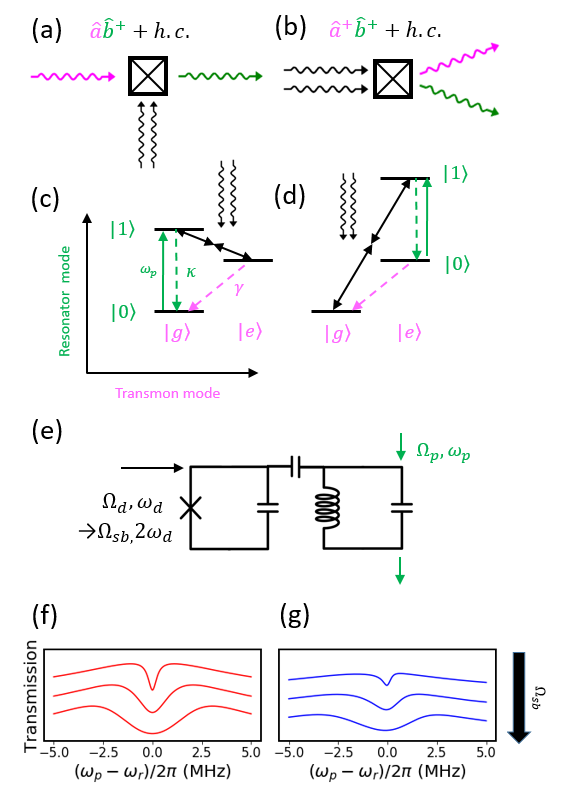
Both the BS and the TMS interaction are schematically described in Fig. 1a and Fig. 1b. Two black-wavy arrows indicate the two-photon drive. Fig. 1c and Fig. 1d denote energy diagram descriptions. In all of the descriptions, the resonator and the transmon mode are colored green and magenta, respectively. In addition to the two-photon drive, we have a weak probe field (green) through the resonator mode to estimate through the resonator’s response. The decay rates of both modes are and , respectively. The energy levels of the resonator mode are denoted by , , ,… and those of the transmon mode are denoted by , ,…
Fig. 1e depicts a simplified circuit diagram of the system. We drive the transmon mode through a direct driveline and we probe the resonator mode through another feedline coupled to the resonator. Fig. 1f and Fig. 1g show how the probe transmission through the resonator varies with increasing for both BS (f) and TMS (g) interaction. The curves are obtained by solving a numerical model based on Eq. 5 with dissipation operators. The decay rates of the resonator and transmon modes in the calculation are MHz and kHz. These parameters are similar to those in the experiment. is set by 2, 4, and 6 MHz in both BS and TMS interaction. The detailed information on the experimental setup and device is provided in Appendix C.1.
In the experiment, we deliberately design a large to facilitate the detection of the interactions through the resonator’s transmission, even with small . Our system satisfies the condition for electromagnetically induced transparency (EIT) eit as long as is smaller than . In this regime, and the other parameters independently shape the transparency window in the middle of the transmission spectrum of the resonator. Thereby, we extract by fitting the resonator’s transmission. The resonator’s linewidth is overwhelmingly larger than the linewidth of the qubit and therefore the system is in the EIT condition as long as is less than around 10 MHz.
The observed are 6.8112 and 4.0755 GHz, respectively. The observed is MHz and can be deduced by . Since the resonator has a broad linewidth, we cannot simply extract from the photon number by splitting the resonator or the transmon spectrum. We obtained 497 kHz from another calibration method in Appendix C.2. From these observations, we can calculate the system’s parameters in Eq. 1 and Eq. 2. The obtained values are GHz and MHz.
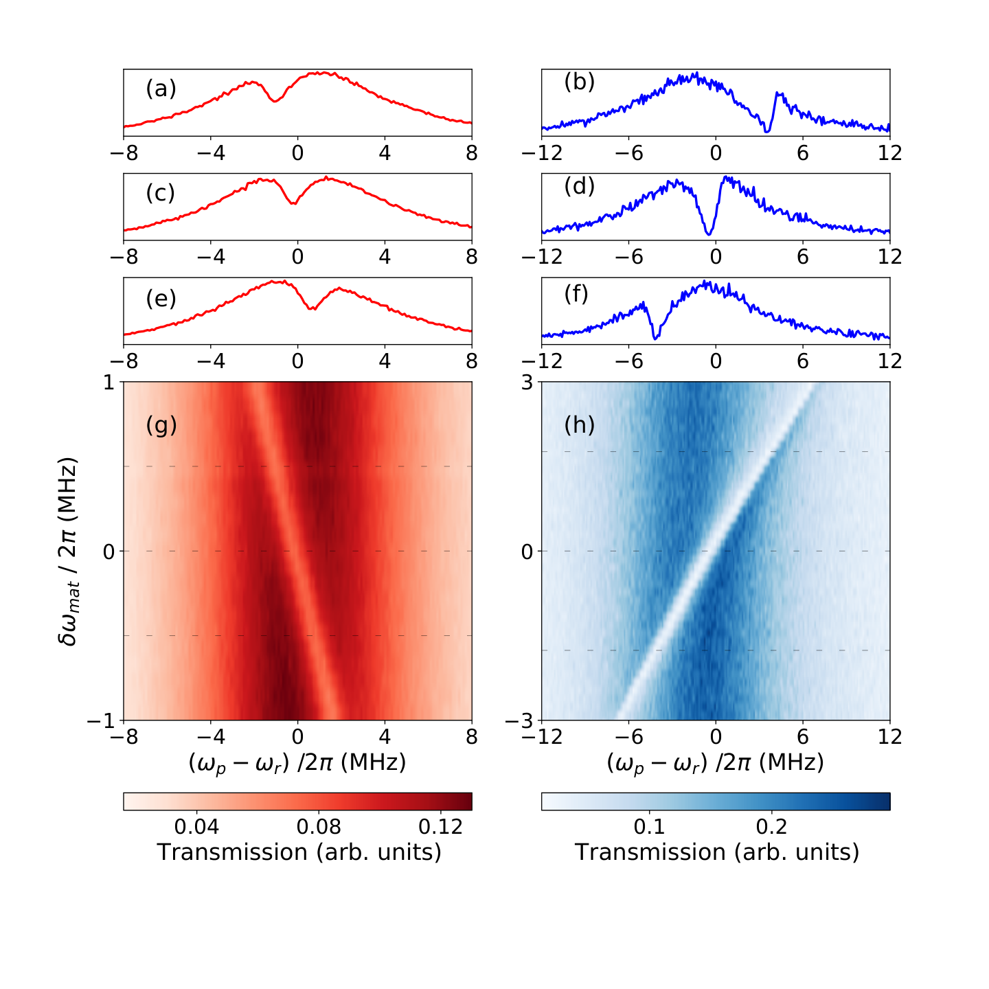
In Fig. 2, we present the procedure used for determining the frequency matching conditions. We define that satisfies for both the BS and TMS interactions. In reality, the resonances undergo shifts, and in our system we have . Thus, we have modified matching conditions, . We swept the driving frequency and find the condition . We obtain the matching conditions when the transparency window is located at the center in the transmission spectrum. More quantitatively, can be obtained by extracting when fitting the transmission data with numerical model given in Appendix A.3. Roughly, 1.36 and 5.44 GHz are expected for both the BS and the TMS interaction, respectively. For the BS interaction, is extremely far off-resonant ( 0.6). This regime of the driving parameter has not been explored. Meanwhile, for TMS interaction, is relatively closer to the RWA regime ( 0.11).
In Fig. 3 a–b, we plot a portion of the transmission spectrum observed in the experiment. We scan the sideband driving power preserving the condition . The solid curves are the fits based on the numerical model that we used in Fig. 1f–g. In the fitting process, the free parameters are , and , while the other parameters are fixed. As we increase the driving amplitudes, we can readily see that the transparency windows behave as expected from Fig. 1f–g. In Fig. 3c, we plot with respect to the corresponding , both of which are extracted from the fitting. The statistical errors in extracting from the fitting are around only 1%, and thus not presented in the figures. We can find a linear correlation between and . The slope of the solid line is obtained from Eq. 6, with no free parameters. It is of note that both BS and TMS data lie on the same theoretical plot, although the driving parameters for each lives in distinct regimes.
To directly identify the breakdown of the RWA, we need to calibrate from an independent method not relying on the transmon frequency shifts. If we know the microwave power at the device (), and the coupling rate between the transmon and drive line (), then is simply given by . However, the uncertainty in the driveline attenuation sets a challenge. An error of only 1 dB in the attenuation induces a 10 error in , which is critical to our study. In future research, this challenge can be circumvented by using an additional ‘sensor’ qubit, as recently demonstrated in Zhou-PRAppl-2020.
IV Numerical simulation
We performed a comprehensive numerical analysis with the experimental conditions. We simulated the system’s time domain dynamics by solving the without including any dissipation. is the density matrix of the system. As in the experiment, we swept the driving frequency for a given and find the frequency where a full oscillation takes place in transitions (BS) or (TMS). is then given by the frequency of the oscillation. More detailed descriptions on the method of the numerical simulation are given in Appendix B.
In Fig. 4, we present the numerical calculation results (circles, triangles and squares) and corresponding analytical calculation results (solid, dashed, and dotted lines). The circles and solid lines refer to the results with the . In the plots, triangles and squares refer to the simulation results dropping the counter-rotating and co-rotating driving terms in . The analytical calculation is based on the Eq. 6. The dashed and dotted lines are obtained by Eq. 7 and Eq. 8, respectively.
In Fig. 4a–b, we compare the sideband transition rates obtained by the numerical simulations (circles, triangles, and squares) with the analytically calculated values (solid, dashed, and dotted lines). In Fig. 4 c–d, we present the frequency shifts of the transmon mode under the matching conditions for given the driving amplitudes in x-axes. The driving frequencies for each data points are set to satisfy the matching conditions for the given driving amplitudes. Although the RWA significantly distorts the and , the breakdown of the RWA is not visible in the versus relation, as seen in Fig. 4 e-f. The simulation data with the RWA perfectly lie on the data without the RWA. Therefore, a careful treatment is required when estimating through or . Relying on the RWA results in significant overestimation of .
V Conclusion
In summary, we performed the quantitative investigation of two-photon assisted four-wave interactions in a superconducting circuit. Over the entire range of the driving amplitudes in this work, our theoretical, numerical and experimental values agree with each other, which suggests that the faithful quantitative estimation of sideband transition rates is possible. This work expands our understanding in the strongly driven quantum systems. The findings through this work are not restricted to the system that we investigate here.
Kerr or Duffing type nonlinearity ubiquitously appears in many physics disciplines other than circuit QED, such as nonlinear optics, cavity optomechanics, and atomic physics Yurke-JOASB-1987; Bose-PRA-1997; Ludwig-PRL-2012; Gupta-PRL-2007. Therefore, we believe our findings can influence a variety of types of research. This work also uses multi-photon assisted transition, which is widely adopted when a desired transition is dipole forbidden Eckhardt-PRL-1962; Hansch-PRL-1975; Eles-JCP-2004; Blais-PPA-2006; Wallraf-PRL-2007; Deppe-NPhys-2008; Leek-PRB-2009; Leek-PRL-2010; Kumar-Ncomm-2016; Premaratne-Ncomm-2017; Vepsalainen-SciAdv-2019; He-NPhys-2019; Meiling-JPCC-2019; Gasparinetti-PRL-2017; Gasparinetti-PRA-2020. From the perspective that the studies of multi-photon transition beyond the RWA are mainly limited to theoretical cases Quattropani-PRA-1982; Saiko-JETP-2006; Meath-JCP-2018, our work would attract attention.
Acknowledgements.
We thank David Theron and Jochem Baselmans for providing us with NbTiN film. Byoung-moo Ann acknowledges support from the European Union’s Horizon 2020 research and innovation program under the Marie Sklodowska-Curie grant agreement No. 722923 (OMT). This project also has received funding from the European Union’s Horizon 2020 research and innovation programme under grant agreement No. 828826 - Quromorphic. The data that support the findings of this study are available in data.Appendix A Theoretical descriptions
A.1 List of symbols
Tab. 1 lists and defines the symbols that are used in the main text and supplemental material.
| Symbol | Meaning |
|---|---|
| Mode frequencies in uncoupled mode basis (Eq. (1) in the main text). | |
| Mode frequencies in normal mode basis (Eq. (2) in the main text). | |
| Experimentally observed mode frequencies (Eq. (5) in the main text). | |
| Driving frequency. | |
| Driving amplitude. | |
| Probe frequency. | |
| Probe amplitude. | |
| Duffing nonlinearities of each modes. | |
| Anharmonicities of each modes. | |
| Cross-anharmonicity (). | |
| Transmon mode annihilation operator in uncoupled mode basis. | |
| Resonator mode annihilation operator in uncoupled mode basis. | |
| Transmon mode annihilation operator in normal mode basis. | |
| Resonator mode annihilation operator in normal mode basis. | |
| Frequency shifts of both modes under driving. | |
| Frequency shifts of both modes under driving. | |
| Sideband transition matching frequency without considering frequency shifts of modes. | |
| Sideband transition matching considering frequency shifts of modes. | |
| - . | |
| Sideband transition rate. | |
| Decay rate of the transmon mode. | |
| Decay rate of the resonator mode. |
A.2 Schrieffer–Wolff transformation
We perturbatively diagonalize the total Hamiltonian by applying the unitary transformation SW to the total Hamiltonian , where and are defined in the main text. The transformed Hamiltonian is given by,
| (9) |
Here, and . simply displaces the field operator () by -(-). Finally, can be expressed by,
| (10) |
For given , collecting the non-rotating terms at the transmon and resonator rotating frame in Eq. 10 yields Tab. 2. We only list the terms that represent the interactions between different modes or the frequency shifts of each mode.
| Operator (+ h.c) | Magnitude ( |
| ||
|
|
None | |||
|
|
None | |||
A.3 Modeling transmission spectrum
The resonator transmission spectrum is proportional to . Here, is a steady state density matrix of the transmon and resonator system, and indicates trace over the transmon states. can be calculated based on the below Eq. 11,
| (11) |
is the Hamiltonian of the prove field. is defined by . is the decay rate of the resonator mode, and is that of the transmon mode. We neglect the pure dephasing rate of the transmon mode. Since we employ a single Josephson junction design, it is expected that the coherence time of the transmon mode is only limited to the decay time. For a steady state, we have , then we can calculate from Eq. 11.
Transmission spectrum is a function of a set of variables (, , , , , , , , , and ). Here, is the independent variable in the fitting process. We fix , , , , and by the values we obtain from the independent measurement without driving field. These quantities are hardly shifted under the driving. is given by the experiment. The free fitting parameters are , , , and . These quantities are extracted from the fitting process.
Appendix B Numerical simulations

.
In this section, we describe the detail procedures of the time-domain numerical simulations. The dynamics of the system are governed by the equation, , where and follow the same definition in the main text. Here, is density matrix of the transmon and resonator. We do not take the dissipation into consideration in the time-domain dynamic simulations. Fig. 5a shows the simulated dynamics (blue line) when the driving frequency satisfies the matching condition for two-mode squeezing (TMS) interaction. The system parameters used in the simulation are the same with the experimental conditions. The sideband drive (, green line) is given as a pulse with 10-ns of Gaussian rising and falling. The arrow indicates the length of the pulse. Fig. 5b shows the area enclosed by the dashed square in Fig. 5a. One can identify the qubit and resonator states significantly vary during the rising and falling duration of the sideband pulse. In Fig. 5c, we sweep the length of the sideband pulse and plot the states of the system at the end of the pulse. We obtain a clear sinusoidal curve. Fig. 5d shows the area enclosed by the dashed square in Fig. 5c.
We sweep the driving frequency for each simulation data point and find the optimal frequency that yields the resonant sideband transitions. This procedure is described in Fig. 6. We chose the when the oscillation has a maximum contrast. We present the simulation data with different driving Hamiltonian in Fig. 7. The solid lines refer to the results with a full driving Hamiltonian containing both co- and counter-rotating terms. The dotted lines (dashed lines) are obtained by the simulations with only co-rotating (counter-rotating) terms in the driving Hamiltonian. See the caption for the detail conditions in the simulations.
Appendix C Experimental methods
C.1 Experimental setup
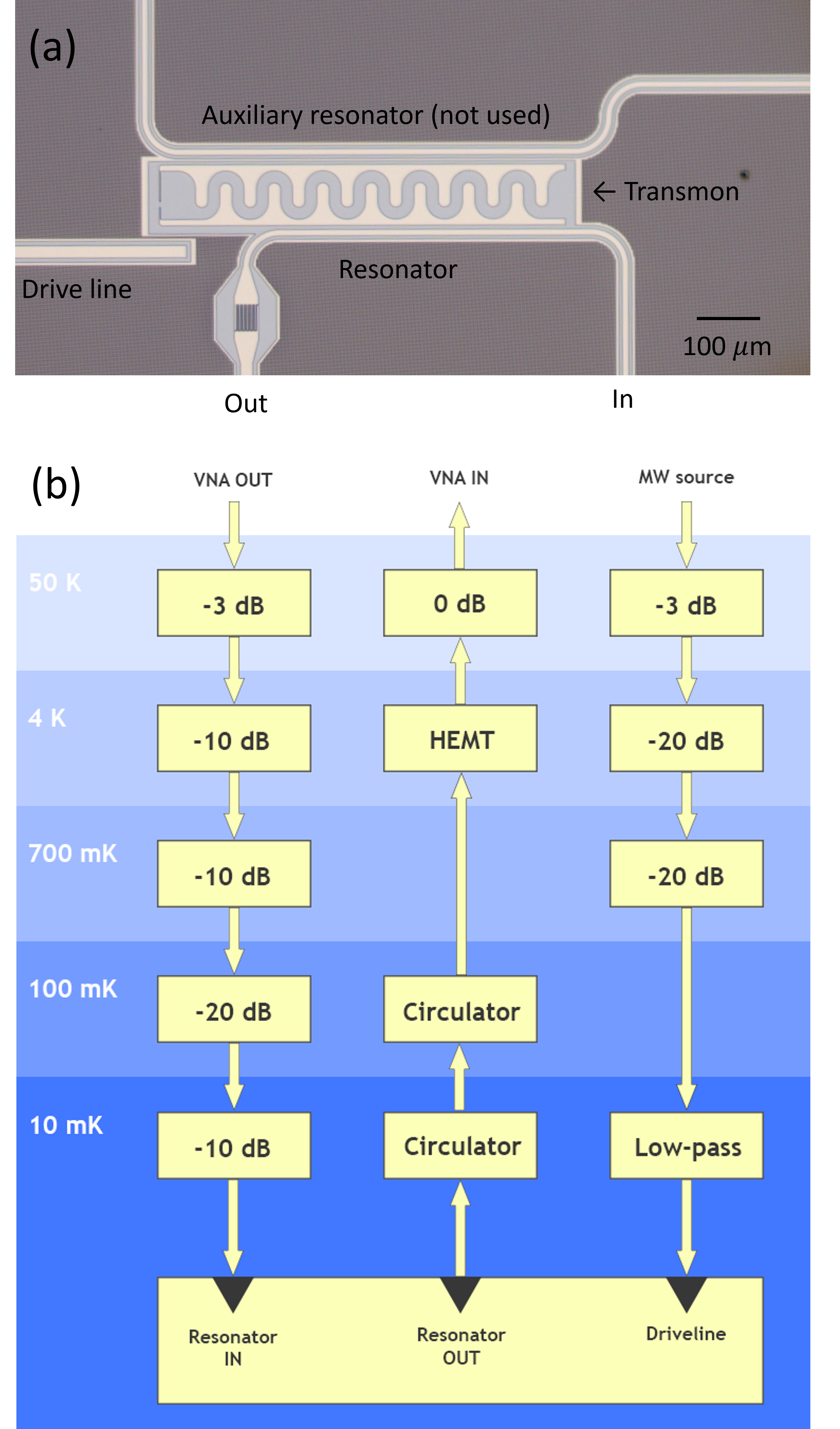
An optical microscope image of the device is given in Fig. 8a. The device is comprised of a transmon and two co-planar waveguide resonators. The design of the device is the same as the one used in our previous work bann-2020. Only one of the resonators was used in this experiment. In addition, there is a drive line directly coupled to the transmon. The base layer of the circuit is fabricated from 100 nm niobium titanium nitride (NbTiN) film on a Silicon substrate. The detailed procedure to prepare the NbTiN film is described in SRON. The transmon is comprised of a Al-AlOx-Al Josephson junction and a finger capacitor. The transmon is not flux tuneable and therefore the frequency is insensitive to the external magnetic field noise.
A cryogenic wiring diagram and measurement electronics are given in Fig. 8b. The device is mounted at the mixing chamber plate of a Bluefors LD-400 dilution fridge. The temperature of the plate is around 10 mK during the measurements. The device is enclosed within a cylindrical cooper shield to block the infrared radiation. To block the external magnetic fields, the copper can is enclosed by a Aluminum shield and two Mu-metal shields. The shields are not represented in the figure. We used a vector network analyzer (Keysight N5222A) to measure the resonator transmissions. An additional microwave source (Keysight N5183B) was used for sideband drivings. We used a non-dissipative low pass filter (Minicircuit VFL-3800+) in the drive line (third column).
C.2 Device parameter extraction

.
In this section, we provide the procedure to calibrate the cross-anharmonicity () between the transmon and resonator modes in the experiment. We use the fact that the EIT transmission spectrum of the resonator depends on the in the nonlinear response regime. In Fig. 9, we simulate the resonator’s transmission spectrum with a beam splitter interaction ( 1.2 MHz). The model that we used in the simulation is based on Eq. (3) in the main text including dissipation operators. In addition, we set by -300 kHz. In the simulation, the linewidths of the resonator and transmon modes are the same with those in the experiment. We simulate in both linear response (Fig. 9a) and nonlinear response (Fig. 9b) regimes. In the linear response regime, we cannot distinguish the from the transmission. Meanwhile, the effect of the is prominent in the nonlinear response regime.
Fig. 10a shows the measured resonator transmission spectrum while sweeping the probe power. is the resonator probe power measured at the output port of the vector network analyzer (VNA). Note that the contrast of the transparency window near the center decreases with increasing probe power. We first fit the resonator’s transmission data in the linear response regime (solid line), setting , , , and as free parameters. Then, we fit the data in the nonlinear response regime (dashed line) while fixing all the parameters obtained from the first fitting and only and are free fitting parameters. When fitting the data in the linear response regime, we set and = 10 kHz. The choice of can be justified since we already know hardly affects the transmission in the linear response regime. The fitting results in both regimes are given in Fig. 10b and Fig. 10c. We obtain = 497 kHz and = 4.35 MHz from the data in the nonlinear regime.
We can also obtain from the fact that the resonator’s transition frequency depends on the transmon’s quantum states Blais-PPA-2006. Fig. 11 shows how the resonator’s transmission spectrum changes as we populate the transmon’s first excited state. We drive the transmon mode with its resonant frequency and increase the power until we cannot see any further shift in the resonator’s frequency. With this drive power, we can approximate the transmon’s state 50:50 mixed state between the ground and first excited states. We observe a frequency shift of 520 kHz, which can be interpreted as .
extracted from Fig. 11 is slightly larger than the value obtained from Fig. 10. The discrepancy of the expected sideband transition rates based on both is about 2 percent. In the main text, we use = kHz obtained from Fig. 10. This approach is advantageous because we can extract the resonator probe power and simultaneously, and consequently it guarantees more consistency.
C.3 Transmon decay rate analysis
In the fitting process to extract the sideband transition rates, the free fitting parameters other than are and . We also present the extracted values for and in data. In this section, we especially focus on the . Fig. 12 shows the fitted (dots) with respect to corresponding . These values are consistent with the from the low power two-tone spectroscopy (dashed line) in general. For BS interaction case, some data points far deviate from the dashed line. We attribute this to the undesired higher order sideband interactions. The matching frequency for BS interaction is close to the matching frequency for single-photon assisted sideband interaction between and . Since the resonator mode has a much larger decay rate, this undesired interaction can increase the effective decay rate of the transmon mode. The rightmost two data of TMS interaction case also far deviate from the solid line. We cannot find the systematic reason for the discrepancy. We could attribute this to the fluctuation of the transmon’s decay rate with respect to time.
Appendix D Additional analytical and numerical analysis
In this section, we confirm that Eq. 6 more accurately predicts the and than Eq. 4. In Fig. 13, we compare the analytical calculation based on Eq. 4 and numerical simulation results in Fig. 4. We can clearly see the discrepancy between the analytical and numerical results becomes larger than that in Fig. 4.
In Fig 14, we perform the additional simulation with various system parameters and compare the numerically simulated sideband transition rates (-Sim) to the theoretical calculations (-Th). We compare two different theoretical approaches based on Eq. 4 and Eq. 6, respectively. Aside from one case (Fig 14-d), -Th based on Eq. 6 are closer to -Sim. Even in Fig 14-d, -Th based on Eq. 6 is more accurate with low driving amplitudes.
References
- (1) F. Bloch and A. Siegert, Magnetic Resonance for Nonrotating Fields, Phys. Rev. 57, 522 (1940).
- (2) P. Giscard et al. Dynamics of Quantum Systems Driven by Time-varying Hamiltonians: Solution for the Bloch-Siegert Hamiltonian and Applications to NMR, Phys. Rev. Research. 2, 023081 (2020).
- (3) I. I. Rabi et al. Use of Rotating Coordinates in Magnetic Resonance Problems, Rev. Mod. Phys. 26, 167 (1954).
- (4) Rotating wave approximation (RWA) is also available for time-independent Hamiltonian in the lab frame. In this case, dropping energy non-conservative terms constitutes the RWA. Nonetheless, we confine the scope of this work to when the breakdown of the RWA results from the time-periodical driving terms.
- (5) D. A. Andrews et al. Observation of Bloch-Siegert Shifts in the 2-2 Microwave Resonance in Atomic Hydrogen, J. Phys. B 8, 1415 (1975).
- (6) G. D. Fuchs et al. Gigahertz Dynamics of a Strongly Driven Single Quantum Spin, Science 326, 5959 (2009).
- (7) J. Tuorila et al. Stark Effect and Generalized Bloch-Siegert Shift in a Strongly Driven Two-Level System, Phys. Rev. Lett. 105, 257003 (2010).
- (8) C. Deng et al. Observation of Floquet States in a Strongly Driven Artificial Atom, Phys. Rev. Lett. 115, 133601 (2015).
- (9) A. Laucht et al. Breaking the Rotating Wave Approximation for a Strongly Driven Dressed Single-electron Spin, Phys. Rev. B 94, 161302(R) (2016).
- (10) I. Pietikäinen et al. Observation of the Bloch–Siegert Shift in a Driven Quantum-to-classical Transition, Phys. Rev. B 96, 020501(R) (2016).
- (11) E. J. Sie et al. Large, Valley-exclusive Bloch-Siegert Shift in Monolayer WS2, Science 355, 6329 (2017).
- (12) J. V. Koski et al. Floquet Spectroscopy of a Strongly Driven Quantum Dot Charge Qubit with a Microwave Resonator, Phys. Rev. Lett. 121, 043603 (2018).
- (13) J. Koch et al. Charge-insensitive Qubit Design Derived from the Cooper Pair Box, Phys. Rev. A 76, 042319 (2007).
- (14) L. Verney et al. Structural Instability of Driven Josephson Circuits Prevented by an Inductive Shunt, Phys. Rev. Appl. 11, 024003 (2019).
- (15) P. J. Leek et al. Using Sideband Transitions for Two-qubit Operations in Superconducting Circuits, Phys. Rev. B 79, 180511(R) (2009).
- (16) P. J. Leek et al. Cavity Quantum Electrodynamics with Separate Photon Storage and Qubit Readout Modes, Phys. Rev. Lett. 104, 100504 (2010).
- (17) M. J. Reagor, Superconducting Cavities for Circuit Quantum Electrodynamics, Yale University, PhD Thesis (2015).
- (18) Z. Leghtas et al. Confining the State of Light to a Quantum Manifold by Engineered Two-photon Loss, Science 347, 853 (2015).
- (19) S. O. Mundhada et al. Experimental Implementation of a Raman-assisted Six-quanta Process , Phys. Rev. Appl. 12, 054051 (2019).
- (20) J. D. Teufel et al. Sideband Cooling of Micromechanical Motion to the Quantum Ground State , Nature 475, 359 (2011).
- (21) A. Schliesser et al. Resolved-sideband Cooling of a Micromechanical Oscillator , Nat. Phys 4, 415 (2008).
- (22) C. Monroe et al. Resolved-Sideband Raman Cooling of a Bound Atom to the 3D Zero-Point Energy , Phys. Rev. Lett. 75, 4011 (1995).
- (23) R. Lescanne et al. Escape of a Driven Quantum Josephson Circuit into Unconfined States , Phys. Rev. Appl. 11, 014030 (2019).
- (24) M. Hennrichh et al. Vacuum-Stimulated Raman Scattering Based on Adiabatic Passage in a High-Finesse Optical Cavity , Phys. Rev. Lett. 85, 4872 (2000).
- (25) G. P. Fedorov et al. Light dressing of a diatomic superconducting artificial molecule , Phys. Rev. A 102, 013707 (2020).
- (26) B. Ann et al. Tunable and Weakly Invasive Probing of a Superconducting Resonator Based on Electromagnetically Induced Transparency , Phys. Rev. A 102, 053721 (2020).
- (27) M. Gely et al. Nature of the Lamb Shift in Weakly Anharmonic Atoms , Phys. Rev. A 98, 053808 (2018).
- (28) K. M. Birnbaum et al., Photon Blockade in an Aptical Cavity with One Trapped Atom , Nature 436, 87 (2005).
- (29) J. R. Schrieffer and P. A. Wolff, Relation Between the Anderson and Kondo Hamiltonians, Phys. Rev. 149, 491 (1966)
- (30) B. Yurke, Squeezed-state Generation Using a Josephson Parametric Amplifier, J. Opt. Soc. Am. B 4, 1551 (1987).
- (31) S. Bose et al. Preparation of Nonclassical States in Cavites with a Moving Mirrow, Phys. Rev. A 56, 4175 (1997).
- (32) M. Lugwig et al. Enhanced Quantum Nonlinearities in a Two-mode Optomechanical System, Phys. Rev. Lett. 109, 063601 (2012).
- (33) S. Gupta et al. Cavity Nonlinear Optics at Low Photon Number from Collective Atomic Motion, Phys. Rev. Lett. 99, 231601 (2007).
- (34) G. Eckhardt et al. Stimulated Raman Scattering From Organic Liquids, Phys. Rev. Lett. 9, 455 (1962).
- (35) T. Hänsch et al. Doppler-Free Two-Photon Spectroscopy of Hydrogen 1S-2S, Phys. Rev. Lett. 34, 307 (1975).
- (36) P. T. Eles et al. Two-photon Two-color Nuclear Magnetic Resonance, J. Chem. Phys. 121, 10167 (2004).
- (37) A. Blais et al. Quantum-information Processing with Circuit Quantum Electrodynamics , Phys. Rev. A 75, 032329 (2007).
- (38) A. Wallraf et al. Sideband Transitions and Two-Tone Spectroscopy of a Superconducting Qubit Strongly Coupled to an On-Chip Cavity, Phys. Rev. Lett. 99, 050501 (2007).
- (39) F. Deppe et al. Two-photon Probe of the Jaynes–Cummings Model and Controlled Symmetry Breaking in Circuit QED, Nat. Phys 4, 686 (2008).
- (40) S. Gasparinetti et al. Correlations and Entanglement of Microwave Photons Emitted in a Cascade Decay, Phys. Rev. Lett. 119, 140504 (2017).
- (41) S. Gasparinetti et al. Two-photon Resonance Fluorescence of a Ladder-type Atomic System, Phys. Rev. A 100, 033802 (2020).
- (42) K. S. Kumar et al. Stimulated Raman Adiabatic Passage in a Three-level Superconducting Circuit, Nat. Comm 7, 10628 (2016).
- (43) S. Premaratne et al. Microwave Photon Fock State Generation by Stimulated Raman Adiabatic Passage, Nat. Comm 8, 14148 (2017).
- (44) A. Vepsäläinen et al. Superadiabatic Population Transfer in a Three-level Superconducting Circuit, Sci. Adv 5, 5999 (2019).
- (45) T. T. Meiling et al. Two-Photon Excitation Fluorescence Spectroscopy of Quantum Dots: Photophysical Properties and Application in Bioassays, J. Phys. Chem. C 112, 9641 (2019)
- (46) Y. -M. He et al. Coherently Driving a Single Quantum Two-level System with Dichromatic Laser Pulses, Nat. Phys 15, 941 (2019).
- (47) A. Quattropani et al. Two-photon Transitions to Excited States in Atomic Hydrogen, Phys. Rev. A 6, 3079 (1982).
- (48) A. P. Saiko et al. Effective Field and the Bloch-Siegert Shift at Bichromatic Excitation of Multiphoton EPR, JETP Letters 84, 130 (2006).
- (49) W. J. Meath, Bloch-Siegert Effects in Two-photon Excitations: Fixed Laser-molecule Configurations Versus Orientational Averaging, J. Chem. Phys. 149, 204114 (2018).
- (50) Y. Zhou et al. Tunable Microwave Single-Photon Source Based on Transmon Qubit with High Efficiency, Phys. Rev. Appl. 13, 034007 (2020).
- (51) B. Ann and G. A. Steele Tunable and Weakly Invasive Probing of a Superconducting Resonator Based on Electromagnetically Induced Transparency , Phys. Rev. A 102, 102, 053721 (2020).
- (52) D. J. Thoen, B. G. C. Bos, E. A. F. Haalebos, T. M. Klapwijk, J. J. A. Baselmans, and A. Endo , Superconducting NbTiN Thin Films with Highly Uniform Properties Over a Ø 100 mm Wafer, IEEE Transactions on Applied Superconductivity, 27, 1500505 (2017).
- (53) B. Ann (2020). Sideband Transitions in a Two-mode Josephson Circuit Driven Beyond the Rotating Wave Approximation. https://doi.org/10.5281/zenodo.4568937.