1Introduction

Robust and Private Learning of Halfspaces

Badih Ghazi Ravi Kumar Pasin Manurangsi Thao Nguyen

Google Research Mountain View, CA {badihghazi, ravi.k53}@gmail.com, {pasin, thaotn}@google.com

Abstract

In this work, we study the trade-off between differential privacy and adversarial robustness under $L_{2}$ -perturbations in the context of learning halfspaces. We prove nearly tight bounds on the sample complexity of robust private learning of halfspaces for a large regime of parameters. A highlight of our results is that robust and private learning is harder than robust or private learning alone. We complement our theoretical analysis with experimental results on the MNIST and USPS datasets, for a learning algorithm that is both differentially private and adversarially robust.

1 Introduction

In this work, we study the interplay between two topics at the core of AI ethics and safety: privacy and robustness.

As modern machine learning models are trained on potentially sensitive data, there has been a tremendous interest in privacy-preserving training methods. Differential privacy (DP) (Dwork et al. 2006b; Dwork et al. 2006a) has emerged as the gold standard for rigorously tracking the privacy leakage of algorithms in general (see, e.g., Dwork and Roth 2014; Vadhan 2017, and the references therein), and machine learning models in particular (Abadi et al. 2016, e.g.,), resulting in several practical deployments in recent years (Erlingsson et al. 2014; Shankland 2014; Greenberg 2016; Apple Differential Privacy Team 2017; Ding et al. 2017; Abowd 2018, e.g.,).

Another vulnerability of machine learning models that has also been widely studied recently is with respect to adversarial manipulations of their inputs at test time, with the intention of causing classification errors (Dalvi et al. 2004; Biggio et al. 2013; Szegedy et al. 2014; Goodfellow et al. 2015; Papernot et al. 2016, e.g.,). Numerous methods have been proposed with the goal of training models that are robust to such adversarial attacks (Madry et al. 2018; Gowal et al. 2018; Gowal et al. 2019; Schott et al. 2019, e.g.,), which in turn has led to new attacks being devised in order to fool these models (Athalye et al. 2018; Carlini and Wagner 2018; Sharma and Chen 2017). See (Kolter and Madry 2018) for a recent tutorial on this topic.

Some recent work has suggested incorporating mechanisms from DP into neural network training to enhance adversarial robustness (Lecuyer et al. 2019; Phan et al. 2020; Phan et al. 2019). Given this existing interplay between DP and robustness, we seek to answer the following natural question:

Is achieving privacy and adversarial robustness
harder than achieving either criterion alone?

Recent empirical work has provided mixed response to the question (Song et al. 2019b; Song et al. 2019a; Hayes 2020), reporting the success rate of membership inference attacks as a heuristic measure of privacy. Instead, using theoretical analysis and the strict guarantees offered by DP, we formally investigate this question in the classic setting of halfspace learning, and arrive at a near-complete picture.

Background.

In order to present our results, we start by recalling some notions from robust learning in the PAC model. Let $\mathcal{C}\subseteq\{0,1\}^{\mathcal{X}}$ be a (Boolean) hypothesis class on an instance space $\mathcal{X}\subseteq\mathbb{R}^{d}$ . A perturbation is defined by a function $\mathbb{P}:\mathcal{X}\to 2^{\mathcal{X}}$ , where $\mathbb{P}(x)\subseteq\mathcal{X}$ denotes the set of allowable perturbed instances starting from an instance $x$ . The robust risk of a hypothesis $h$ with respect to a distribution $\mathcal{D}$ on $\mathcal{X}\times\{\pm 1\}$ and perturbation $\mathbb{P}$ is defined as $\mathcal{R}_{\mathbb{P}}(h,\mathcal{D})=\Pr_{(\mathbf{x},y)\sim\mathcal{D}}[\exists z\in\mathbb{P}(\mathbf{x}),h(\mathbf{z})\neq y].$ A distribution $\mathcal{D}$ is said to be realizable (with respect to $\mathcal{C}$ and $\mathbb{P}$ ) iff there exists $h^{*}\in\mathcal{C}$ such that $\mathcal{R}_{\mathbb{P}}(h^{*},\mathcal{D})=0$ . In the adversarially robust PAC learning problem, the learner is given i.i.d. samples from a realizable distribution $\mathcal{D}$ on $\mathcal{X}\times\{\pm 1\}$ , and the goal is to output a hypothesis $h:\mathcal{X}\to\{\pm 1\}$ such that with probability $1-\xi$ it holds that $\mathcal{R}_{\mathbb{P}}(h,\mathcal{D})\leq\alpha$ . We refer to $\xi$ as the failure probability and $\alpha$ as the accuracy parameter. A learner is said to be proper if the output hypothesis $h$ belongs to $\mathcal{C}$ ; otherwise, it is said to be improper.

We focus our study on the concept class of halfspaces, i.e., $\mathcal{C}_{\text{halfspaces}}:=\{h_{\mathbf{w}}\mid\mathbf{w}\in\mathbb{R}^{d}\}$ where $h_{\mathbf{w}}(\mathbf{x})=\sgn(\left<\mathbf{w},\mathbf{x}\right>)$ , in this model with respect to $L_{2}$ perturbations, i.e., $\mathbb{P}_{\gamma}(\mathbf{x}):=\{\mathbf{z}\in\mathcal{X}:\|\mathbf{z}-\mathbf{x}\|_{2}\leq\gamma\}$ for margin parameter $\gamma>0$ . We assume throughout that the domain of our functions is bounded in the $d$ -dimensional Euclidean unit ball $\mathbb{B}^{d}:=\{\mathbf{x}\in\mathbb{R}^{d}\mid\|\mathbf{x}\|_{2}\leq 1\}$ . We also write $\mathcal{R}_{\gamma}$ as a shorthand for $\mathcal{R}_{\mathbb{P}_{\gamma}}$ . An algorithm is said to be a $(\gamma,\gamma^{\prime})$ -robust learner if, for any realizable distribution $\mathcal{D}$ with respect to $\mathcal{C}_{\text{halfspaces}}$ and $\mathbb{P}_{\gamma}$ , using a certain number of samples, it outputs a hypothesis $h$ such that w.p. $1-\xi$ , we have $\mathcal{R}_{\gamma^{\prime}}(h,\mathcal{D})\leq\alpha$ , where $\alpha,\xi>0$ are sufficiently smaller than some positive constant. We are especially interested in the case¹¹ 1 It is necessary to have $\gamma^{\prime}<\gamma$ ; when $\gamma=\gamma^{\prime}$ , proper $(\gamma,\gamma^{\prime})$ -robust learning is as hard as general proper learning of halfspace (Diakonikolas et al. 2020, see, e.g.,), which is impossible with any finite number of samples under DP (Bun et al. 2015). where $\gamma^{\prime}$ is close to $\gamma$ ; for simplicity, we use $\gamma^{\prime}=0.9\gamma$ as a representative setting throughout. In robust learning, the main quantities of interest are the sample complexity, i.e., the minimum number of samples needed to learn, and the running time of the learning algorithm.

We use the standard terminology of DP. Recall that two datasets $\mathbf{X}$ and $\mathbf{X}^{\prime}$ are neighbors if $\mathbf{X}^{\prime}$ results from adding or removing a single data point from $\mathbf{X}$ .

Definition 1 (Differential Privacy (DP) (Dwork et al. 2006b; Dwork et al. 2006a)).

Let $\epsilon,\delta\in\mathbb{R}_{\geq 0}$ . A randomized algorithm $\mathbb{A}$ taking as input a dataset is said to be $(\epsilon,\delta)$ -differentially private (denoted by $(\epsilon,\delta)$ -DP) if for any two neighboring datasets $\mathbf{X}$ and $\mathbf{X}^{\prime}$ , and for any subset $S$ of outputs of $\mathbb{A}$ , it is the case that $\Pr[\mathbb{A}(\mathbf{X})\in S]\leq e^{\epsilon}\cdot\Pr[\mathbb{A}(\mathbf{X}^{\prime})\in S]+\delta$ . If $\delta=0$ , $\mathbb{A}$ is said to be $\epsilon$ -differentially private (denoted by $\epsilon$ -DP).

As usual, $\epsilon$ should be thought of as a small constant, whereas $\delta$ should be negligible in the dataset size. We refer to the case where $\delta=0$ as pure-DP, and the case where $\delta>0$ as approximate-DP.

Our Results.

		Robust		Non-robust
	Bounds	Proper	Improper	Proper	Improper
Non-private	Tight	$\Theta(1/\gamma^{2})$
Pure-DP	Upper	$O(d)$ (Theorem 5)		$\tilde{O}(1/\gamma^{2})$
Pure-DP	Lower	$\Omega(d)$ (Theorem 2)		$\Omega(1/\gamma^{2})$	$\Omega(1/\gamma^{2})$ (Theorem 4)
Approximate-DP	Upper	$\tilde{O}(\sqrt{d}/\gamma)$ ^†		$\tilde{O}(1/\gamma^{2})$
Approximate-DP	Lower	$\Omega(\sqrt{d}/\gamma)$ (Theorem 3)	$\Omega(1/\gamma^{2})$ (Theorem 4)	$\Omega(1/\gamma^{2})$ (Theorem 4)

Table 1: Trade-offs between privacy and robustness. The robust column corresponds to

(\gamma,0.9\gamma)

-robust learners, whereas the non-robust column corresponds to

(\gamma,0)

-robust learners. For simplicity of presentation, we assume

\alpha,\epsilon,\xi\in(0,1)

are sufficiently small constants,

d\geq 1/\gamma^{2}

, and for approximate-DP lower bounds, that

\delta=o(1/n)

. While approximate-DP upper bounds (marked with^†) can already be derived from previous work, we give a faster algorithm (Theorem 6). For DP, known results are from (Nguyen et al. 2020); for the non-private case, the results follow, e.g., from (Bartlett and Mendelson 2002; Koltchinskii and Panchenko 2002).

We assume that $\epsilon\leq O(1)$ unless otherwise stated, and that $\gamma,\alpha,\xi>0$ are sufficiently smaller than some positive constant. We will not state these assumptions explicitly here for simplicity; interested readers may refer to (the first lines of) the proofs for the exact upper bounds that are imposed.

We first prove that robust learning with pure-DP requires $\Omega(d)$ samples.

Theorem 2.

Any $\epsilon$ -DP $(\gamma,0.9\gamma)$ -robust (possibly improper) learner has sample complexity $\Omega(d/\epsilon)$ .

In the private but non-robust setting (i.e., for an $\epsilon$ -DP $(\gamma,0)$ -robust learner²² 2 This means that the output hypothesis only needs to have a small classification error, but may have a large robust risk.), Nguyen et al. 2020 showed that $O(1/\gamma^{2})$ samples suffice. Together with earlier known results showing that $(\gamma,0.9\gamma)$ -robust learning (without privacy) only requires $O(1/\gamma^{2})$ samples (Bartlett and Mendelson 2002; Koltchinskii and Panchenko 2002, e.g.,), our result gives a separation between robust private learning and private learning alone or robust learning alone, whenever $d\gg 1/\gamma^{2}$ .

For the case of approximate-DP, we establish a lower bound of $\Omega(\min\{\sqrt{d}/\gamma,d\})$ , which holds only against proper learners. As for Theorem 2 in the context of pure-DP, this result implies a similar separation in the approximate-DP proper learning setting.

Theorem 3.

Let $\epsilon<1$ . Any $(\epsilon,o(1/n))$ -DP $(\gamma,0.9\gamma)$ -robust proper learner has sample complexity $n=\Omega(\min\{\sqrt{d}/\gamma,d\})$ .

Our proof technique can also be used to improve the lower bound for DP $(\gamma,0)$ -robust learning. Specifically, Nguyen et al. 2020 show an $\Omega(1/\gamma^{2})$ lower bound for proper $(\gamma,0)$ -robust learners with pure-DP. We extend it to hold even for improper $(\gamma,0)$ -robust learners with approximate-DP:

Theorem 4.

For any $\epsilon>0$ , there exists $\delta>0$ such that any $(\epsilon,\delta)$ -DP $(\gamma,0)$ -robust (possibly improper) learner has sample complexity $\Omega\left(\frac{1}{\epsilon\gamma^{2}}\right)$ . Moreover, this holds even when $d=O(1/\gamma^{2})$ .

Finally, we provide algorithms with nearly matching upper bounds. For pure-DP, we prove the following, which matches the lower bound in Theorem 2 to within a constant factor when $d\geq 1/\gamma^{2}$ .

Theorem 5.

There is an $\epsilon$ -DP $(\gamma,0.9\gamma)$ -robust learner with sample complexity³³ 3 Here $O_{\alpha}(\cdot)$ hides a factor of $\poly(1/\alpha)$ , and $\tilde{O}(\cdot)$ hides a factor of $\poly\log(1/(\alpha\gamma\delta))$ . $O_{\alpha}\left(\frac{1}{\epsilon}\max\{d,\frac{1}{\gamma^{2}}\}\right)$ .

For approximate-DP, it is already possible⁴⁴ 4 This can be achieved by running the DP ERM algorithm of (Bassily et al. 2014) with the hinge loss; see (Nguyen et al. 2020) for the analysis. to achieve a sample complexity³³footnotemark: 3 of $n=\tilde{O}_{\alpha}(\sqrt{d}/\gamma)$ (Nguyen et al. 2020; Bassily et al. 2014) but the running time is $\Omega(n^{2}d)$ .⁵⁵ 5 Specifically, Nguyen et al. 2020 uses the DP empirical risk minimization algorithm of (Bassily et al. 2014) with the hinge loss; however, the latter requires $\Omega(n^{2})$ iterations and each iteration requires $\Omega(d)$ time. We give a faster algorithm with running time $O_{\alpha}(nd/\gamma)$ .

Theorem 6.

There is an $(\epsilon,\delta)$ -DP $(\gamma,0.9\gamma)$ -robust learner with sample complexity $n=\tilde{O}_{\alpha}\left(\frac{1}{\epsilon}\cdot\max\left\{\frac{\sqrt{d}}{\gamma},\frac{1}{\gamma^{2}}\right\}\right)$ and running time $\tilde{O}_{\alpha}\left(nd/\gamma\right)$ .

Our theoretical results and those from prior works are summarized in Table 1. Notice that the non-private robust setting and the non-robust private setting each requires only $O(1/\gamma^{2})$ samples, whereas our results show that the private and robust setting requires either $\Omega(d)$ samples (for pure-DP) or $\Omega(\sqrt{d}/\gamma)$ samples (for approximate-DP). This separation positively answers the question central to our study.

We complement our theoretical results by empirically evaluating our algorithm (from Theorem 6) on the MNIST (LeCun et al. 2010) and USPS (Hull 1994) datasets. Our results show that it is possible to achieve both robustness and privacy guarantees while maintaining reasonable performance. We further provide evidence that models trained via our algorithm are more resilient to adversarial noise compared to neural networks trained via DP-SGD (Abadi et al. 2016).

Organization.

In the two following sections, we describe in detail the ideas behind each of our proofs. We then present our experimental results in Section 4. Finally, we discuss additional related work and several open questions in Sections 5 and 6 respectively. Due to space constraints, all missing proofs and additional experiments are deferred to the Supplementary Material.

2 Sample Complexity Lower Bounds

In this section, we explain the high-level ideas behind each of our sample complexity lower bounds. Our pure-DP lower bound is based on a packing framework and our approximate-DP lower bounds are based on fingerprinting codes.

2.1 Pure-DP Lower Bound (Theorem 2)

We use the packing framework, a DP lower bound proof technique that originated in (Hardt and Talwar 2010). Roughly speaking, to apply this framework, we have to construct many input distributions for which the sets of valid outputs for each distribution are disjoint (hence the name “packing”). In our context, this means that we would like to construct distributions $\mathcal{D}^{(1)},\dots,\mathcal{D}^{(K)}$ such that the sets $G^{(i)}$ of hypotheses with small robust risk on $\mathcal{D}^{(i)}$ are disjoint. Once we have done this, the packing framework immediately gives us a lower bound of $\Omega(\log K/\epsilon)$ on the sample complexity; below we describe a construction for $K=2^{\Omega(d)}$ distributions, which yields the desired $\Omega(d/\epsilon)$ lower bound in Theorem 2.

Our construction proceeds by picking unit vectors $\mathbf{w}^{(1)},\dots,\mathbf{w}^{(K)}$ that are nearly orthogonal, i.e., $\left|\left<\mathbf{w}^{(i)},\mathbf{w}^{(j)}\right>\right|<0.01$ for all $i\neq j$ . It is not hard to see (and well-known) that such vectors exist for $K=2^{\Omega(d)}$ . We then let $\mathcal{D}^{(i)}$ be the uniform distribution on $(1.01\gamma\cdot\mathbf{w}^{(i)},+1),(-1.01\gamma\cdot\mathbf{w}^{(i)},-1)$ .

Now, let $G^{(i)}$ denote the set of hypotheses $h$ for which $\mathcal{R}_{0.9\gamma}(h,\mathcal{D}^{(i)})<0.5$ . Since our distribution $\mathcal{D}^{(i)}$ is uniform on two elements, we must have that $\mathcal{R}_{0.9\gamma}(h,\mathcal{D}^{(i)})=0$ for all $h\in G^{(i)}$ . To see that $G^{(i)}$ and $G^{(j)}$ are disjoint for any $i\neq j$ , notice that, since $\left|\left<\mathbf{w}^{(i)},\mathbf{w}^{(j)}\right>\right|<0.01$ , the point $1.01\gamma\cdot\mathbf{w}^{(i)}$ is within distance $1.8\gamma$ from the point $-1.01\gamma\cdot\mathbf{w}^{(j)}$ . This means that any hypothesis $h$ cannot correctly classify both $(1.01\gamma\cdot\mathbf{w}^{(i)},1)$ and $(-1.01\gamma\cdot\mathbf{w}^{(i)},-1)$ with margin at least $0.9\gamma$ , which implies that $G^{(i)}\cap G^{(j)}=\emptyset$ . This completes our proof sketch.

We end by remarking that the previous work of Nguyen et al. 2020 also uses a packing argument; the main differences between our construction and theirs are in the choice of the distributions $\mathcal{D}^{(i)}$ and the proof of disjointness of the $G^{(i)}$ ’s. Our construction of $\mathcal{D}^{(i)}$ is in fact simpler, since our proof of disjointness can rely on the robustness guarantee. These differences are inherent, since our lower bound holds even against improper learners, i.e., when the output hypothesis may not be a halfspace, whereas the lower bound of Nguyen et al. 2020 only holds against the particular case of proper learners.

2.2 Approximate-DP Lower Bound (Theorem 3)

We reduce from a lower bound from the line of works (Bun et al. 2018; Dwork et al. 2015; Steinke and Ullman 2016; Steinke and Ullman 2017) inspired by fingerprinting codes. Specifically, these works consider the so-called attribute mean problem, where we are given a set of vectors drawn from some (hidden) distribution $\mathcal{D}$ on $\{\pm 1\}^{d}$ and the goal is to compute the mean. It is known that getting an estimate to within 0.1 of the true mean in each coordinate requires $\Omega(\sqrt{d})$ samples. In fact, Steinke and Ullman 2017 show that even outputting a vector with a ‘‘non-trivial’’ dot product⁶⁶ 6 Specifically, this holds when the output vector has $\ell_{2}$ -norm at most $\sqrt{d}$ and the dot product is at least $\zeta d$ for any constant $\zeta>0$ . with the mean already requires $\Omega(\sqrt{d})$ samples. This almost implies our desired lower bound: the only remaining step is to turn $\mathcal{D}$ to a distribution that is realizable with margin $\gamma^{*}$ . We do this by conditioning $\mathcal{D}$ on only points $\mathbf{x}$ with a sufficiently large dot product with the true mean, and then adding both $(\mathbf{x},+1)$ and $(-\mathbf{x},-1)$ to our distribution. This reduction gives an $\Omega(\sqrt{d})$ lower bound on the sample complexity of $(\gamma^{*},0.9\gamma^{*})$ -robust proper learners, for some absolute constant margin parameter $\gamma^{*}>0$ .

To get an improved bound for a smaller margin $\gamma$ , we “embed” $\Omega(1/\gamma^{2})$ hard instances above in each of $O(\gamma^{2}d)$ dimensions. More specifically, let $T=\gamma^{*}/\gamma$ ; for each $i\in[T^{2}]$ we create a distribution $\mathcal{D}^{(i)}$ that is the hard distribution from the previous paragraph in $d^{\prime}:=d/T$ dimensions embedded onto coordinates $d^{\prime}(i-1)+1,\dots,d^{\prime}i$ . We then let the distribution $\mathcal{D}^{\prime}$ be the (uniform) mixture of $\mathcal{D}^{(1)},\dots,\mathcal{D}^{(T^{2})}$ . Since each $\mathcal{D}^{(i)}$ is realizable with margin $\gamma^{*}$ via some halfspace $\mathbf{w}^{(i)}$ , we may take $\mathbf{w}^{*}:=\frac{1}{T}\sum_{i\in[T^{2}]}\frac{\mathbf{w}^{(i)}}{\|\mathbf{w}^{(i)}\|}$ to realize the distribution $\mathcal{D}^{\prime}$ with margin $\frac{1}{T}\cdot\gamma^{*}=\gamma$ as desired.

Now, to find any $\mathbf{w}$ with small $\mathcal{R}_{0.9\gamma}(h_{\mathbf{w}},\mathcal{D}^{\prime})$ , we roughly have to solve (most of) the $T^{2}$ instances $\mathcal{D}^{(i)}$ ’s. Recall that solving each of these instances requires $\Omega(\sqrt{d^{\prime}})$ samples. Thus, the combined instance requires $\Omega(T^{2}\cdot\sqrt{d^{\prime}})=\Omega(1/\gamma^{2}\cdot\sqrt{\gamma^{2}d})=\Omega(\sqrt{d}/\gamma)$ samples.

2.3 Non-Robust DP Learning Lower Bound (Theorem 4)

This lower bound once again uses the “embedding” technique described above. Here we start with a hard one-dimensional instance, which is simply the uniform distribution on $(x,-1),(x,+1)$ where $x$ is either $+1$ or $-1$ . When $\delta>0$ is sufficiently small (depending on $\epsilon$ ), it is simple to show that any $(\epsilon,\delta)$ -DP $(1,0)$ -learner for this instance requires $\Omega(1/\epsilon)$ samples. Similar to the previous proof overview, we embed $1/\gamma^{2}$ such instances into $1/\gamma^{2}$ dimensions. Since the one-dimensional instance requires $\Omega(1/\epsilon)$ samples, the combined instance requires $\Omega(1/(\epsilon\gamma^{2}))$ samples, thereby yielding Theorem 4.

3 Sample-Efficient Algorithms

In this section, we present our algorithms for robust and private learning. Our pure-DP algorithm is based on an improved analysis of the exponential mechanism. Our approximate-DP algorithm is based on a private, batched version of the perceptron algorithm.

In the following discussions, we assume that $\mathbf{w}^{*}$ is an (unknown) optimal halfspace with respect to the input distribution $\mathcal{D}$ and $L_{2}$ -perturbations with margin parameter $\gamma$ , i.e., that $\mathbf{w}^{*}$ satisfies $\mathcal{R}_{\gamma}(h_{\mathbf{w}^{*}},\mathcal{D})=0$ . We may assume without loss of generality that $\|\mathbf{w}^{*}\|=1$ .

3.1 Pure-DP Algorithm (Theorem 5)

Theorem 5 is shown via the exponential mechanism (EM) (McSherry and Talwar 2007). Our guarantee is an improvement over the “straightforward” analysis of EM on a $(0.1\gamma)$ -net of the unit sphere in $\mathbb{R}^{d}$ , which gives an upper bound of $O_{\alpha}(d\log(1/\gamma)/\epsilon)$ (Nguyen et al. 2020). On the other hand, when $d\geq 1/\gamma^{2}$ , our sample complexity is $O_{\alpha}(d/\epsilon)$ . The intuition behind our improvement is that, if we take a random unit vector $\mathbf{w}$ such that $\left<\mathbf{w},\mathbf{w}^{*}\right>\geq 0.99$ , then it already gives a small robust risk (in expectation) when $d\gg 1/\gamma^{2}$ because the component of $\mathbf{w}$ orthogonal to $\mathbf{w}^{*}$ is a random $(d-1)$ -dimensional vector of norm less than one, meaning that in expectation it only affects the margin by $O(1/\sqrt{d})\ll 0.1\gamma$ . Now, a random unit vector satisfies $\left<\mathbf{w},\mathbf{w}^{*}\right>\geq 0.99$ with probability $2^{-O(d)}$ , which (roughly speaking) means that EM should only require $O_{\alpha}(d/\epsilon)$ samples.

3.2 Approximate-DP Algorithm (Theorem 6)

To prove Theorem 6, we use the DP Batch Perceptron algorithm presented in Algorithm 1. DP Batch Perceptron is the batch and privatized version of the so-called margin perceptron algorithm (Duda and Hart 1973; Collobert and Bengio 2004). That is, in each iteration, we randomly sample a batch of samples and for each sample $(\mathbf{x},y)$ in the batch that is not correctly classified with margin $\gamma^{\prime}$ , we add $y\cdot\mathbf{x}$ to the current weight of the halfspace. Furthermore, we add some Gaussian noise to the weight vector to make this algorithm private. We also have a “stopping condition” that terminates whenever the number of samples mislabeled at margin $\gamma^{\prime}$ is sufficiently small. (We add Laplace noise to the number of such samples to make it private.) To get a $(\gamma,0.9\gamma)$ -robust learner, it suffices for us to set, e.g., $\gamma^{\prime}=0.95\gamma$ ; we use this value of $\gamma^{\prime}$ in the subsequent discussions.

DP-Batch-Perceptron

{}_{\gamma^{\prime},p,T,b,\sigma}(\{(\mathbf{x}_{j},y_{j})\}_{j\in[n]})

\mathbf{w}_{0}\leftarrow\mathbf{0}

2: for

i=1,\dots,T

S_{i}\leftarrow

a set of samples where each

(\mathbf{x}_{j},y_{j})

is independently included w.p.

p

M_{i}\leftarrow\emptyset

5: for

(\mathbf{x},y)\in S_{i}

6: if

\sgn\left(\left<\frac{\mathbf{w}_{i-1}}{\|\mathbf{w}_{i-1}\|},\mathbf{x}\right>-y\cdot\gamma^{\prime}\right)\neq y

M_{i}\leftarrow M_{i}\cup\{(\mathbf{x},y)\}

8: Sample

\nu_{i}\sim\Lap(b)

9: if

|M_{i}|+\nu_{i}<0.3\alpha pn

10: return

\mathbf{w}_{i-1}/\|\mathbf{w}_{i-1}\|

11:

\mathbf{u}_{i}\leftarrow\sum_{(\mathbf{x},y)\in M_{i}}y\cdot\mathbf{x}

12: Sample

\mathbf{g}_{i}\sim\mathcal{N}(0,\sigma^{2}\cdot I_{d\times d})

13:

\mathbf{w}_{i}\leftarrow\mathbf{w}_{i-1}+\mathbf{u}_{i}+\mathbf{g}_{i}

return FAIL

Algorithm 1 DP Batch Perceptron

Before we dive into the details of the proof, we remark that our runtime reduction, compared to the generic algorithm from (Bassily et al. 2014), comes from the fact that, in the accuracy analysis, we only need the number of iterations $T$ to be $O_{\alpha}(1/\gamma^{2})$ , similar to the perceptron algorithm (Novikoff 1963). On the other hand, the generic theorem of Bassily et al. 2014 requires $n^{2}=\tilde{O}_{\alpha}(d^{2}/\gamma^{2})$ iterations.

The accuracy analysis of DP Batch Perceptron follows the blueprint of that of perceptron (Novikoff 1963). Specifically, we keep track of the following two quantities: $\left<\mathbf{w}_{i},\mathbf{w}^{*}\right>$ , the dot product between the current halfspace $\mathbf{w}_{i}$ and the “true” halfspace $\mathbf{w}^{*}$ , and $\|\mathbf{w}_{i}\|$ , the (Euclidean) norm of $\mathbf{w}_{i}$ . We would like to show that, after the first few iterations, $\left<\mathbf{w}_{i},\mathbf{w}^{*}\right>$ increases at a faster rate than $\|\mathbf{w}_{i}\|$ . Since $\left<\mathbf{w}_{i},\mathbf{w}^{*}\right>$ is bounded above by $\|\mathbf{w}_{i}\|$ , we may use this to bound the number $T$ of iterations required for the algorithm to converge.

For simplicity, we assume that in each iteration $|M_{i}|$ is equal to $m>0$ . Let us first consider the case where no noise is added (i.e., $\sigma=0$ ). From the definition of $\mathbf{w}^{*}$ , it is simple⁷⁷ 7 Specifically, since $\mathcal{R}_{\gamma}(h_{\mathbf{w}^{*}},\mathcal{D})=0$ , we have $y\left<\mathbf{w}^{*},\mathbf{z}\right>\geq 0$ for all $\mathbf{z}$ such that $\|\mathbf{x}-\mathbf{z}\|\leq\gamma$ . Plugging in $\mathbf{z}=\mathbf{x}-\gamma y\mathbf{w}^{*}$ yields the claimed inequality. to check that $\left<\mathbf{w}^{*},y\cdot\mathbf{x}\right>\geq\gamma$ for all samples $(\mathbf{x},y)$ . This means that $\left<\mathbf{w}^{*},\mathbf{u}_{i}\right>\geq\gamma m$ , resulting in

\displaystyle\left<\mathbf{w}^{*},\mathbf{w}_{i}\right>\geq\left<\mathbf{w}^{*},\mathbf{w}_{i-1}\right>+\gamma m.

(1)

On the other hand, the check condition before we add each example $(\mathbf{x},y)$ to $M_{i}$ (Line 6) ensures that $\left<\mathbf{w}_{i},y\cdot\mathbf{x}\right>\leq\gamma^{\prime}\cdot\|\mathbf{w}_{i}\|$ for all $(\mathbf{x},y)\in M_{i}$ . From this one can derive the following bound:

\displaystyle\|\mathbf{w}_{i}\|\leq\|\mathbf{w}_{i-1}\|+\gamma^{\prime}m+\frac{0.5m^{2}}{\|\mathbf{w}_{i-1}\|},

which, when $\|\mathbf{w}_{i-1}\|\geq 50m/\gamma$ , implies that

\displaystyle\|\mathbf{w}_{i}\|\leq\|\mathbf{w}_{i-1}\|+0.96\gamma m.

(2)

Combining (1) and (2), we arrive at

\displaystyle 50m/\gamma+0.96\gamma mi\geq\|\mathbf{w}_{i}\|\geq\left<\mathbf{w}^{*},\mathbf{w}_{i}\right>\geq\gamma mi.

This implies that the algorithm must stop after $T=O\left(1/\gamma^{2}\right)$ iterations. (When $m=1$ , this noiseless analysis is essentially the same as the original convergence analysis of perceptron (Novikoff 1963).)

The previous paragraphs outlined the analysis for the noiseless case where $\sigma=0$ . Next, we will describe how the noise $\sigma$ affects the analysis and our choices of parameters. Roughly speaking, we would like the inequalities (1) and (2) to “approximately” hold even after adding noise. In particular, this means that we would like the right-hand side of these inequalities to be affected by at most $o(\gamma m)$ by the noise addition, with high probability. This condition will determine our selection of parameters.

For (1), the inclusion of the noise term $\mathbf{g}_{i}$ adds to the right-hand side by $\left<\mathbf{w}^{*},\mathbf{g}_{i}\right>$ . The expectation of this term is $\|\mathbf{w}^{*}\|\cdot\sigma\leq\sigma$ , which means that it suffices to ensure that $m\geq\tilde{\omega}\left(\sigma/\gamma\right)$ . For (2), it turns out that the dominant additional term is $\frac{\|\mathbf{g}_{i}\|^{2}}{\|\mathbf{w}_{i-1}\|}$ which, under the assumption that $\|\mathbf{w}_{i-1}\|\geq 50m/\gamma$ , is at most $O(\gamma\|\mathbf{g}_{i}\|^{2}/m)$ ; this term is $O(\gamma d\sigma^{2}/m)$ in expectation. Since we would like this term to be $o(\gamma m)$ , it suffices to have $m=\tilde{\omega}(\sigma\cdot\sqrt{d})$ . By combining these two requirements, we may pick $m=\sigma\cdot\tilde{\omega}(\sqrt{d}+1/\gamma)$ . We remark that the number of iterations still remains $T=O(1/\gamma^{2})$ , as in the noiseless case above.

While we have so far assumed for simplicity that $|M_{i}|=m$ in all iterations, in the actual analysis we only require that $|M_{i}|\geq m$ . Furthermore, it is simple to show that, as long as the current hypothesis has robust risk significantly more than $\alpha$ , we will have $|M_{i}|\geq\Omega_{\alpha}(pn)$ with high probability. Combining with the previous paragraph, this gives us the following condition (assuming that $\alpha$ is constant):

\displaystyle pn\geq\sigma\cdot\tilde{\omega}(\sqrt{d}+1/\gamma).

This leads us to pick the following set of parameters:

n=\tilde{O}\left(\frac{1}{\gamma}\left(\sqrt{d}+\frac{1}{\gamma}\right)\right),\quad p=\tilde{O}(\gamma),\quad\sigma=\tilde{O}(1).

The privacy analysis of our algorithm is similar to that of DP-SGD (Bassily et al. 2014). Specifically, by the choice of $\sigma=\tilde{O}(1)$ and subsampling rate $p=\tilde{O}(\gamma)$ , each iteration of the algorithm is $\left(O(\gamma\epsilon),O(\gamma^{2}\delta)\right)$ -DP (Dwork et al. 2010; Balle et al. 2018, e.g.,). Since the number of iterations is $T=O(1/\gamma^{2})$ , advanced composition theorem (Dwork et al. 2010) implies that the entire algorithm is $(O(\sqrt{T}\cdot\gamma\epsilon),O(T\cdot\gamma^{2}\delta))$ = $(\epsilon,\delta)$ -DP as desired.

We end by noting that, despite the popularity of perceptron-based algorithms, we are not aware of any work that analyzes the above noised and batched variant. The most closely related analysis we are aware of is that of Blum et al. 2005, whose algorithm uses the entire dataset in each iteration. While it is possible to adapt their analysis to the batch setting, it unfortunately does not give an optimal sample complexity. Specifically, their analysis requires the batch size to be $\Omega(\sqrt{d}/\gamma)$ , resulting in sample complexity of $\Omega(\sqrt{d}/\gamma^{2})$ . On the other hand, our more careful analysis works even with batch size $\tilde{O}(\sqrt{d}+1/\gamma)$ , which results in the desired $\tilde{O_{\alpha,\epsilon}(\sqrt{d}/\gamma)}$ sample complexity when $d\geq 1/\gamma^{2}$ .

4 Experiments

Refer to caption — (a) Accuracy as $\epsilon$ varies

We run our DP Batch Perceptron algorithm on the MNIST (LeCun et al. 2010) and USPS (Hull 1994) datasets, both of which involve 10-class digit classification. We train a separate halfspace classifier $\mathbf{w}^{(y)}$ for each class $y\in\{1,\dots,10\}$ for one epoch. To predict on an image $\mathbf{x}$ , we output a class $y^{*}$ that maximizes $\left<\mathbf{w}^{(y^{*})},\mathbf{x}\right>$ . We tune batch size as a hyperparameter with values 1, 10, 50, 100, 500, 1000, and $\gamma^{\prime}$ with values 1, 0.1, 0.01, 0.001, 0.0001. Each set of experiments is repeated for 20 random trials. To reduce the number of hyperparameters, we slightly modify our algorithm so that we do not stop early (i.e., removing Lines 9 and 10) but instead return the weight vector $w_{T}$ at the end of the $T$ th iteration (where $T$ is set in the algorithm).

The standard deviation $\sigma$ of the Gaussian noise added is determined by a fixed $(\epsilon,\delta)$ -DP budget, computed using Renyi DP (Abadi et al. 2016; Mironov 2017). The calculations for this follow the implementation in the official TensorFlow Privacy repository (https://github.com/tensorflow/privacy). For experiments with varying $\epsilon$ (first column of Figure 1), we fix $\delta$ to $10^{-5}$ for MNIST and $10^{-4}$ for USPS. We observe that despite the robustness and privacy constraints, DP Batch Perceptron still achieves competitive accuracy on both datasets. We also report performance with varying $\delta$ values of $10^{-2},10^{-3},10^{-4},10^{-5}$ (second column of Figure 1), while keeping $\epsilon$ fixed at 1.0.

Adversarial Robustness Evaluation.

We compare the robustness of our models against those of neural networks trained with DP-SGD. For the latter, we follow the architecture found in the official TensorFlow Privacy tutorial, which consists of two convolutional layers, each followed by a MaxPool operation, and a dense layer that outputs predicted logits. The network is then trained with batch size $250$ , learning rate $0.15$ , $L_{2}$ clipping-norm $1.0$ , and for $60$ epochs. This configuration yields competitive performance on the MNIST dataset.

To evaluate the robustness of the models, we calculate the robust risk on the test dataset for varying values of the perturbation norm (i.e., margin) $\gamma$ . Following common practice in the field, we plot the robust accuracy on the test data, which is defined as one minus the robust risk (i.e., $1-\mathcal{R}_{\gamma}(h,\mathcal{D})$ where $\mathcal{D}$ is the test dataset distribution), instead of the robust risk itself. Similarly, our plots use the unnormalized margin, meaning that the images are not re-scaled to have $L_{2}$ norm equal to $1$ before prediction. Note that each of their pixel values is still scaled (i.e., divided by 255 if necessary) to have values in the range [0, 1].

In the case of DP Batch Perceptron, it is known (Hein and Andriushchenko 2017, see, e.g.,) that an example $(\mathbf{x},y)$ cannot be perturbed (using $\mathbb{P}_{\gamma}$ ) to an incorrect label if $\gamma<\min_{y^{\prime}\neq y}\frac{\left<\mathbf{w}^{(y)},\mathbf{x}\right>-\left<\mathbf{w}^{(y^{\prime})},\mathbf{x}\right>}{\|\mathbf{w}^{(y)}-\mathbf{w}^{(y^{\prime})}\|}$ . This formula allows us to exactly calculate the robust risk of our linear classifiers. We stress that this is a provable robustness guarantee, i.e., it holds against all adversarial attacks with perturbation norm (at most) $\gamma$ .

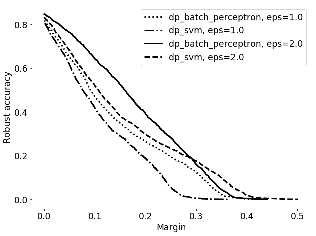
We demonstrate the effect of the change in the required privacy level on the robust risk of our linear classifiers in the right most column of Figure 1. The x-axis of the plots represents the parameter $\gamma$ and the y-axis represents the $\gamma$ -robust accuracy on the test dataset.

In contrast to linear models, there is no efficiently-computable formula to calculate robust risk for general neural networks. In this case, we use a variant of a popular adversarial robustness attack (outlined below) to estimate the robust risk of DP-SGD-trained neural networks. Unlike the linear classifier case, this method only gives a lower bound on the robust risk, meaning that more sophisticated attacks might result in even more incorrect classifications.

We now briefly summarize the attack we use against DP-SGD-trained neural networks; (a version of) this method was already presented in (Szegedy et al. 2014). Let $M$ denote a trained model; recall that the last layer of our model consists of 10 outputs corresponding to each class and to predict an image we take $y^{*}$ with the maximum output. Given a sample $(\mathbf{x},y)$ , we would like to determine whether there exists a perturbation $\Delta\in\mathbb{R}^{d}$ with $\|\Delta\|\leq\gamma$ such that $M$ predict $\mathbf{x}+\Delta$ to be some other class $y^{\prime}\neq y$ . Instead of solving this (intractable) problem directly, the attack considers a modified objective of

\displaystyle\min_{\|\Delta\|\leq\gamma}\ell(M(\mathbf{x}+\Delta),y^{\prime})

where $\ell$ is some loss function. This optimization problem is then solved using Projected Gradient Descent (PGD). We use the cross entropy loss in our attack.

Comparisons of the robust accuracy of models trained via DP Batch Perceptron and those trained via DP-SGD are shown in Figure 2 for $\delta=10^{-5}$ and $\epsilon=0.5,1,2$ . In the case of $\epsilon=0.5$ , while both classifiers have similar test accuracies (without any perturbation, $\gamma=0$ ), as $\gamma$ increases, the robust accuracy rapidly degrades for the DP-SGD-trained neural network compared to that of the DP Batch Perceptron model. This overall trend persists for $\epsilon=1,2$ ; in both cases, the neural networks start off with noticeably larger test accuracy when $\gamma=0$ but are eventually surpassed by halfspace classifiers as $\gamma$ increases.

5 Other Related Work

Learning Halfspaces with Margin.

$L_{2}$ robustness is a classical setting closely related to the notion of margin (Rosenblatt 1958; Novikoff 1963, e.g.,). (See the supplementary material for formal definitions.) Known margin-based learning methods include the classic perceptron algorithm (Rosenblatt 1958; Novikoff 1963) and its many generalizations and variants (Duda and Hart 1973; Collobert and Bengio 2004; Freund and Schapire 1999; Gentile and Littlestone 1999; Li and Long 2002; Gentile 2001, e.g.,), as well as Support Vector Machines (SVMs) (Boser et al. 1992; Cortes and Vapnik 1995). A number of works also explore a closely related agnostic setting, where the distribution $\mathcal{D}$ is not guaranteed to be realizable with a margin (Ben-David and Simon 2000; Shalev-Shwartz et al. 2010; Long and Servedio 2011; Birnbaum and Shalev-Shwartz 2012; Diakonikolas et al. 2019; Diakonikolas et al. 2020, e.g.,).

Generalization aspects of margin-based learning of halfspaces is also a widely studied topic (Bartlett 1998; Zhang 2002; Bartlett and Mendelson 2002; Koltchinskii and Panchenko 2002; McAllester 2003; Kakade et al. 2008, e.g.,), and it is known that the sample complexity of robust learning of halfspaces is $O(1/(\alpha\gamma)^{2})$ (Bartlett and Mendelson 2002; Koltchinskii and Panchenko 2002).

To the best of our knowledge, the first work that combines the study of learning halfspaces with margin and DP is (Nguyen et al. 2020); their results are represented in Table 1. Recently, Ghazi et al. 2020 gave alternative proofs for some results of Nguyen et al. 2020 via reductions to clustering problems, but these do not provide any improved sample complexity or running time.

Adversarially Robust Learning.

There has been a rapidly growing literature on adversarial robustness. Some of these works have presented evidence that training robust classifiers might be harder than non-robust ones (Awasthi et al. 2019; Bubeck et al. 2018; Bubeck et al. 2019; Degwekar et al. 2019, e.g.,). Other works aim to demonstrate the accuracy cost of robustness (Tsipras et al. 2019; Raghunathan et al. 2019, e.g., ). Another line of work seeks to determine the right quantity that governs adversarial generalization (Schmidt et al. 2018; Montasser et al. 2019; Khim and Loh 2018; Yin et al. 2019; Awasthi et al. 2020, e.g.,).

Differentially Private Learning.

Private learning has been a popular topic since the early days of differential privacy (Kasiviswanathan et al. 2008, e.g.,)). Apart from the work of Nguyen et al. 2020 on privately learning halfspaces with a margin, a line of work closely related to our setting is the study of the sample complexity of learning threshold functions (Beimel et al. 2016; Feldman and Xiao 2014; Bun et al. 2015; Alon et al. 2019; Kaplan et al. 2020a) and halfspaces (Beimel et al. 2019; Kaplan et al. 2020b; Kaplan et al. 2020c). These works study the setting where the unit ball $\mathbb{B}^{d}$ is discretized so that the domain $\mathcal{X}$ is $X^{d}\cap\mathbb{B}^{d}$ (i.e., each coordinate is an element of $X$ ). Interestingly, it has been shown that when $X$ is infinite, halfspaces become unlearnable, i.e., the sample complexity becomes unbounded (Alon et al. 2019). On the other hand, an $(\epsilon,o(1/n))$ -DP learner with sample complexity $\tilde{O}\left(\frac{d^{2.5}}{\alpha\epsilon}\right)\cdot 2^{O(\log^{*}|X|)}$ exists (Kaplan et al. 2020b).

While the above setting is not directly comparable to ours, it is possible to reduce between the margin setting and the discretized setting, albeit with some loss. For example, we may use the grid discretization with $|X|=0.01\gamma/\sqrt{d}$ , to obtain a $(\gamma,0)$ -learner with sample complexity $\tilde{O}\left(\frac{d^{2.5}}{\alpha\epsilon}\right)\cdot 2^{O(\log^{*}(1/\gamma))}$ . This is better than the (straightforward) bound of $O(d\cdot\log(1/\gamma))$ obtained by applying the exponential mechanism (McSherry and Talwar 2007) when $\gamma$ is very small (e.g., $\gamma\leq 2^{-d^{1.6}}$ ). It remains an interesting open problem to close such a gap for very small values of $\gamma$ .

Several works (Rubinstein et al. 2012; Chaudhuri et al. 2011, e.g.,) have studied differentially private SVMs. However, to the best of our knowledge, there is no straightforward way to translate their theoretical results to those shown in our paper as the objectives in the two settings are different.

6 Conclusions and Future Directions

In this work, we prove new trade-offs, measured in terms of sample complexity, between privacy and robustness—two crucial properties within the domain of AI ethics and safety—for the classic task of halfspace learning. Our theoretical results demonstrate that DP and adversarially robust learning requires a larger number of samples than either DP or adversarially robust learning alone. We then propose a learning algorithm that meets both criteria, and test it on two multi-class classification datasets. We also provide empirical evidence that despite having a slight advantage in terms of test accuracy on the main task, standard neural networks trained with DP-SGD are not as robust as those trained with our algorithm.

We conclude with a few future research directions. First, it would be interesting to close the gap for the sample complexity of improper approximate-DP $(\gamma,0.9\gamma)$ -robust learners; for $d\gg 1/\gamma^{2}$ , the upper bound is $O(\sqrt{d}/\gamma)$ (Theorem 6) but the lower bound is only $\Omega(1/\gamma^{2})$ (Theorem 4). This is the only case where there is still a super-polylogarithmic gap for $d\gg 1/\gamma^{2}$ .

Another technical open question is to improve the lower bounds in Theorem 3 to $\Omega(\min\{\sqrt{d}/\gamma,d\})/\epsilon$ . Currently, we are missing the $\epsilon$ term because we invoke a lower bound from Steinke and Ullman 2017 (Theorem 11), which was specifically proved only for $\epsilon=1$ .

Furthermore, it would be natural to extend our study to $L_{p}$ perturbations for $p\neq 2$ . An especially noteworthy case is when $p=\infty$ , which is a well-studied setting in the adversarial robustness literature.

Finally, it would be very interesting to provide a theoretical understanding of private and robust learning beyond halfspaces, to accommodate complex algorithms (e.g., deep neural networks) that are better suited for more challenging tasks.

References

Abadi et al. (2016) Martin Abadi, Andy Chu, Ian Goodfellow, H Brendan McMahan, Ilya Mironov, Kunal Talwar, and Li Zhang. Deep learning with differential privacy. In CCS, pages 308–318, 2016.
Abowd (2018) John M Abowd. The US Census Bureau adopts differential privacy. In KDD, pages 2867–2867, 2018.
Alon et al. (1990) Noga Alon, Oded Goldreich, Johan Håstad, and René Peralta. Simple constructions of almost $k$ -wise independent random variables. In FOCS, pages 544–553, 1990.
Alon et al. (2019) Noga Alon, Roi Livni, Maryanthe Malliaris, and Shay Moran. Private PAC learning implies finite Littlestone dimension. In STOC, pages 852–860, 2019.
Apple Differential Privacy Team (2017) Apple Differential Privacy Team. Learning with privacy at scale. Apple Machine Learning Journal, 2017.
Athalye et al. (2018) Anish Athalye, Nicholas Carlini, and David Wagner. Obfuscated gradients give a false sense of security: Circumventing defenses to adversarial examples. In ICML, pages 274–283, 2018.
Awasthi et al. (2019) Pranjal Awasthi, Abhratanu Dutta, and Aravindan Vijayaraghavan. On robustness to adversarial examples and polynomial optimization. In NeurIPS, pages 13760–13770, 2019.
Awasthi et al. (2020) Pranjal Awasthi, Natalie Frank, and Mehryar Mohri. Adversarial learning guarantees for linear hypotheses and neural networks. In ICML, pages 431–441, 2020.
Balle et al. (2018) Borja Balle, Gilles Barthe, and Marco Gaboardi. Privacy amplification by subsampling: Tight analyses via couplings and divergences. In NeurIPS, pages 6280–6290, 2018.
Bartlett (1998) Peter L. Bartlett. The sample complexity of pattern classification with neural networks: The size of the weights is more important than the size of the network. IEEE Trans. Inf. Theory, 44(2):525–536, 1998.
Bartlett and Mendelson (2002) Peter L Bartlett and Shahar Mendelson. Rademacher and Gaussian complexities: Risk bounds and structural results. JMLR, 3:463–482, 2002.
Bassily et al. (2014) Raef Bassily, Adam D. Smith, and Abhradeep Thakurta. Private empirical risk minimization: Efficient algorithms and tight error bounds. In FOCS, pages 464–473, 2014.
Bassily et al. (2019) Raef Bassily, Vitaly Feldman, Kunal Talwar, and Abhradeep Guha Thakurta. Private stochastic convex optimization with optimal rates. In NeurIPS, pages 11282–11291, 2019.
Beimel et al. (2016) Amos Beimel, Kobbi Nissim, and Uri Stemmer. Private learning and sanitization: Pure vs. approximate differential privacy. Theory Comput., 12(1):1–61, 2016.
Beimel et al. (2019) Amos Beimel, Shay Moran, Kobbi Nissim, and Uri Stemmer. Private center points and learning of halfspaces. In COLT, pages 269–282, 2019.
Ben-David and Simon (2000) Shai Ben-David and Hans Ulrich Simon. Efficient learning of linear perceptrons. In NIPS, pages 189–195, 2000.
Biggio et al. (2013) Battista Biggio, Igino Corona, Davide Maiorca, Blaine Nelson, Nedim Šrndić, Pavel Laskov, Giorgio Giacinto, and Fabio Roli. Evasion attacks against machine learning at test time. In ECML/PKDD, pages 387–402, 2013.
Birnbaum and Shalev-Shwartz (2012) Aharon Birnbaum and Shai Shalev-Shwartz. Learning halfspaces with the zero-one loss: Time-accuracy tradeoffs. In NIPS, pages 935–943, 2012.
Blum et al. (2005) Avrim Blum, Cynthia Dwork, Frank McSherry, and Kobbi Nissim. Practical privacy: the SuLQ framework. In PODS, pages 128–138, 2005.
Boser et al. (1992) Bernhard E. Boser, Isabelle Guyon, and Vladimir Vapnik. A training algorithm for optimal margin classifiers. In COLT, pages 144–152, 1992.
Bubeck et al. (2018) Sébastien Bubeck, Yin Tat Lee, Eric Price, and Ilya Razenshteyn. Adversarial examples from computational constraints. In ICML, pages 831–840, 2018.
Bubeck et al. (2019) Sébastien Bubeck, Yin Tat Lee, Eric Price, and Ilya Razenshteyn. Adversarial examples from computational constraints. In ICML, pages 831–840, 2019.
Bun et al. (2015) Mark Bun, Kobbi Nissim, Uri Stemmer, and Salil Vadhan. Differentially private release and learning of threshold functions. In FOCS, pages 634–649, 2015.
Bun et al. (2018) Mark Bun, Jonathan Ullman, and Salil P. Vadhan. Fingerprinting codes and the price of approximate differential privacy. SIAM J. Comput., 47(5):1888–1938, 2018.
Carlini and Wagner (2018) Nicholas Carlini and David Wagner. Audio adversarial examples: Targeted attacks on speech-to-text. In IEEE SPW, pages 1–7, 2018.
Chaudhuri et al. (2011) Kamalika Chaudhuri, Claire Monteleoni, and Anand D Sarwate. Differentially private empirical risk minimization. JMLR, 12(3):1069–1109, 2011.
Collobert and Bengio (2004) Ronan Collobert and Samy Bengio. Links between perceptrons, MLPs and SVMs. In ICML, 2004.
Cortes and Vapnik (1995) Corinna Cortes and Vladimir Vapnik. Support-vector networks. Mach. Learn., 20(3):273–297, 1995.
Dalvi et al. (2004) Nilesh Dalvi, Pedro Domingos, Sumit Sanghai, and Deepak Verma. Adversarial classification. In KDD, pages 99–108, 2004.
Degwekar et al. (2019) Akshay Degwekar, Preetum Nakkiran, and Vinod Vaikuntanathan. Computational limitations in robust classification and win-win results. In COLT, pages 994–1028, 2019.
Diakonikolas et al. (2019) Ilias Diakonikolas, Daniel Kane, and Pasin Manurangsi. Nearly tight bounds for robust proper learning of halfspaces with a margin. In NeurIPS, pages 10473–10484, 2019.
Diakonikolas et al. (2020) Ilias Diakonikolas, Daniel M. Kane, and Pasin Manurangsi. The complexity of adversarially robust proper learning of halfspaces with agnostic noise. In NeurIPS, 2020.
Ding et al. (2017) Bolin Ding, Janardhan Kulkarni, and Sergey Yekhanin. Collecting telemetry data privately. In NIPS, pages 3571–3580, 2017.
Duda and Hart (1973) Richard O. Duda and Peter E. Hart. Pattern Classification and Scene Analysis. Wiley, 1973.
Dwork and Roth (2014) Cynthia Dwork and Aaron Roth. The algorithmic foundations of differential privacy. Foundations and Trends in Theoretical Computer Science, 9(3-4):211–407, 2014.
Dwork et al. (2006a) Cynthia Dwork, Krishnaram Kenthapadi, Frank McSherry, Ilya Mironov, and Moni Naor. Our data, ourselves: Privacy via distributed noise generation. In EUROCRYPT, pages 486–503, 2006a.
Dwork et al. (2006b) Cynthia Dwork, Frank McSherry, Kobbi Nissim, and Adam D. Smith. Calibrating noise to sensitivity in private data analysis. In TCC, pages 265–284, 2006b.
Dwork et al. (2010) Cynthia Dwork, Guy N. Rothblum, and Salil P. Vadhan. Boosting and differential privacy. In FOCS, pages 51–60, 2010.
Dwork et al. (2015) Cynthia Dwork, Adam D. Smith, Thomas Steinke, Jonathan Ullman, and Salil P. Vadhan. Robust traceability from trace amounts. In FOCS, pages 650–669, 2015.
Erlingsson et al. (2014) Úlfar Erlingsson, Vasyl Pihur, and Aleksandra Korolova. RAPPOR: Randomized aggregatable privacy-preserving ordinal response. In CCS, pages 1054–1067, 2014.
Feldman and Xiao (2014) Vitaly Feldman and David Xiao. Sample complexity bounds on differentially private learning via communication complexity. In COLT, pages 1000–1019, 2014.
Feldman et al. (2020) Vitaly Feldman, Tomer Koren, and Kunal Talwar. Private stochastic convex optimization: optimal rates in linear time. In STOC, pages 439–449, 2020.
Freund and Schapire (1999) Yoav Freund and Robert E. Schapire. Large margin classification using the perceptron algorithm. Mach. Learn., 37(3):277–296, 1999.
Gentile (2001) Claudio Gentile. A new approximate maximal margin classification algorithm. JMLR, 2:213–242, 2001.
Gentile and Littlestone (1999) Claudio Gentile and Nick Littlestone. The robustness of the p-norm algorithms. In COLT, pages 1–11, 1999.
Ghazi et al. (2020) Badih Ghazi, Ravi Kumar, and Pasin Manurangsi. Differentially private clustering: Tight approximation ratios. In NeurIPS, 2020.
Goodfellow et al. (2015) Ian J Goodfellow, Jonathon Shlens, and Christian Szegedy. Explaining and harnessing adversarial examples. In ICLR, 2015.
Gowal et al. (2018) Sven Gowal, Krishnamurthy Dvijotham, Robert Stanforth, Rudy Bunel, Chongli Qin, Jonathan Uesato, Relja Arandjelovic, Timothy Mann, and Pushmeet Kohli. On the effectiveness of interval bound propagation for training verifiably robust models. arXiv Preprint:1810.12715, 2018.
Gowal et al. (2019) Sven Gowal, Jonathan Uesato, Chongli Qin, Po-Sen Huang, Timothy Mann, and Pushmeet Kohli. An alternative surrogate loss for PGD-based adversarial testing. arXiv Preprint: 1910.09338, 2019.
Greenberg (2016) Andy Greenberg. Apple’s “differential privacy” is about collecting your data – but not your data. Wired, June, 13, 2016.
Hardt and Talwar (2010) Moritz Hardt and Kunal Talwar. On the geometry of differential privacy. In STOC, pages 705–714, 2010.
Hayes (2020) Jamie Hayes. Provable trade-offs between private & robust machine learning. arXiv Preprint: 2006.04622, 2020.
Hein and Andriushchenko (2017) Matthias Hein and Maksym Andriushchenko. Formal guarantees on the robustness of a classifier against adversarial manipulation. In NeurIPS, pages 2266–2276, 2017.
Hull (1994) Jonathan J. Hull. A database for handwritten text recognition research. IEEE PAMI, 16(5):550–554, 1994.
Kakade et al. (2008) Sham M. Kakade, Karthik Sridharan, and Ambuj Tewari. On the complexity of linear prediction: Risk bounds, margin bounds, and regularization. In NIPS, pages 793–800, 2008.
Kaplan et al. (2020a) Haim Kaplan, Katrina Ligett, Yishay Mansour, Moni Naor, and Uri Stemmer. Privately learning thresholds: Closing the exponential gap. In COLT, pages 2263–2285, 2020a.
Kaplan et al. (2020b) Haim Kaplan, Yishay Mansour, Uri Stemmer, and Eliad Tsfadia. Private learning of halfspaces: Simplifying the construction and reducing the sample complexity. In NeurIPS, 2020b.
Kaplan et al. (2020c) Haim Kaplan, Micha Sharir, and Uri Stemmer. How to Find a Point in the Convex Hull Privately. In SoCG, pages 52:1–52:15, 2020c.
Kasiviswanathan et al. (2008) Shiva Prasad Kasiviswanathan, Homin K. Lee, Kobbi Nissim, Sofya Raskhodnikova, and Adam D. Smith. What can we learn privately? In FOCS, pages 531–540, 2008.
Khim and Loh (2018) Justin Khim and Po-Ling Loh. Adversarial risk bounds via function transformation. arXiv Preprint: 1810.09519, 2018.
Koltchinskii and Panchenko (2002) Vladimir Koltchinskii and Dmitry Panchenko. Empirical margin distributions and bounding the generalization error of combined classifiers. The Annals of Statistics, 30(1):1–50, 2002.
Kolter and Madry (2018) Zico Kolter and Aleksander Madry. Adversarial robustness: Theory and practice. Tutorial at NeurIPS, 2018.
Laurent and Massart (2000) Beatrice Laurent and Pascal Massart. Adaptive estimation of a quadratic functional by model selection. Annals of Statistics, pages 1302–1338, 2000.
Lecun et al. (1998) Yann Lecun, Léon Bottou, Yoshua Bengio, and Patrick Haffner. Gradient-based learning applied to document recognition. In Proceedings of the IEEE, pages 2278–2324, 1998.
LeCun et al. (2010) Yann LeCun, Corinna Cortes, and CJ Burges. MNIST handwritten digit database, 2010. http://yann.lecun.com/exdb/mnist.
Lecuyer et al. (2019) Mathias Lecuyer, Vaggelis Atlidakis, Roxana Geambasu, Daniel Hsu, and Suman Jana. Certified robustness to adversarial examples with differential privacy. In IEEE S&P, pages 656–672, 2019.
Li and Long (2002) Yi Li and Philip M. Long. The relaxed online maximum margin algorithm. Mach. Learn., 46(1-3):361–387, 2002.
Long and Servedio (2011) Philip M. Long and Rocco A. Servedio. Learning large-margin halfspaces with more malicious noise. In NIPS, pages 91–99, 2011.
Madry et al. (2018) Aleksander Madry, Aleksandar Makelov, Ludwig Schmidt, Dimitris Tsipras, and Adrian Vladu. Towards deep learning models resistant to adversarial attacks. In ICLR, 2018.
McAllester (2003) David A. McAllester. Simplified PAC-Bayesian margin bounds. In COLT, pages 203–215, 2003.
McSherry and Talwar (2007) Frank McSherry and Kunal Talwar. Mechanism design via differential privacy. In FOCS, pages 94–103, 2007.
Mironov (2017) Ilya Mironov. Rényi differential privacy. In CSF, pages 263–275, 2017.
Montasser et al. (2019) Omar Montasser, Steve Hanneke, and Nathan Srebro. VC classes are adversarially robustly learnable, but only improperly. In COLT, pages 2512–2530, 2019.
Nguyen et al. (2020) Huy Le Nguyen, Jonathan Ullman, and Lydia Zakynthinou. Efficient private algorithms for learning large-margin halfspaces. In ALT, pages 704–724, 2020.
Novikoff (1963) Albert B Novikoff. On convergence proofs for perceptrons. Technical report, Stanford Research Institute, Menlo Park, CA, 1963.
Papernot et al. (2016) Nicolas Papernot, Patrick McDaniel, and Ian Goodfellow. Transferability in machine learning: from phenomena to black-box attacks using adversarial samples. arXiv Preprint: 1605.07277, 2016.
Phan et al. (2019) NhatHai Phan, Minh Vu, Yang Liu, Ruoming Jin, Dejing Dou, Xintao Wu, and My T Thai. Heterogeneous Gaussian mechanism: Preserving differential privacy in deep learning with provable robustness. In IJCAI, pages 4753–4759, 2019.
Phan et al. (2020) NhatHai Phan, My T Thai, Han Hu, Ruoming Jin, Tong Sun, and Dejing Dou. Scalable differential privacy with certified robustness in adversarial learning. In ICML, pages 7683–7694, 2020.
Raghunathan et al. (2019) Aditi Raghunathan, Sang Michael Xie, Fanny Yang, John C Duchi, and Percy Liang. Adversarial training can hurt generalization. arXiv Preprint: 1906.06032, 2019.
Rahimi and Recht (2007) Ali Rahimi and Benjamin Recht. Random features for large-scale kernel machines. In NIPS, pages 1177–1184, 2007.
Rosenblatt (1958) Frank Rosenblatt. The perceptron: a probabilistic model for information storage and organization in the brain. Psychological Review, 65(6):386, 1958.
Rubinstein et al. (2012) Benjamin IP Rubinstein, Peter L Bartlett, Ling Huang, and Nina Taft. Learning in a large function space: Privacy-preserving mechanisms for SVM learning. J. Priv. Confidentiality, 4(1), 2012.
Schmidt et al. (2018) Ludwig Schmidt, Shibani Santurkar, Dimitris Tsipras, Kunal Talwar, and Aleksander Madry. Adversarially robust generalization requires more data. In NeurIPS, pages 5014–5026, 2018.
Schölkopf et al. (1997) Bernhard Schölkopf, Kah Kay Sung, Christopher J. C. Burges, Federico Girosi, Partha Niyogi, Tomaso A. Poggio, and Vladimir Vapnik. Comparing support vector machines with Gaussian kernels to radial basis function classifiers. IEEE Trans. Signal Process., 45(11):2758–2765, 1997.
Schott et al. (2019) Lukas Schott, Jonas Rauber, Matthias Bethge, and Wieland Brendel. Towards the first adversarially robust neural network model on MNIST. In ICLR, 2019.
Shalev-Shwartz et al. (2010) Shai Shalev-Shwartz, Ohad Shamir, and Karthik Sridharan. Learning kernel-based halfspaces with the zero-one loss. In COLT, pages 441–450, 2010.
Shankland (2014) Stephen Shankland. How Google tricks itself to protect Chrome user privacy. CNET, October, 2014.
Sharma and Chen (2017) Yash Sharma and Pin-Yu Chen. Attacking the Madry defense model with $l_{1}$ -based adversarial examples. arXiv Preprint: 1710.10733, 2017.
Song et al. (2019a) Liwei Song, Reza Shokri, and Prateek Mittal. Membership inference attacks against adversarially robust deep learning models. In IEEE SPW, pages 50–56, 2019a.
Song et al. (2019b) Liwei Song, Reza Shokri, and Prateek Mittal. Privacy risks of securing machine learning models against adversarial examples. In CCS, pages 241–257, 2019b.
Steinke and Ullman (2016) Thomas Steinke and Jonathan Ullman. Between pure and approximate differential privacy. J. Priv. Confidentiality, 7(2), 2016.
Steinke and Ullman (2017) Thomas Steinke and Jonathan Ullman. Tight lower bounds for differentially private selection. In FOCS, pages 552–563, 2017.
Szegedy et al. (2014) Christian Szegedy, Wojciech Zaremba, Ilya Sutskever, Joan Bruna, Dumitru Erhan, Ian Goodfellow, and Rob Fergus. Intriguing properties of neural networks. In ICLR, 2014.
Tsipras et al. (2019) Dimitris Tsipras, Shibani Santurkar, Logan Engstrom, Alexander Turner, and Aleksander Madry. Robustness may be at odds with accuracy. In ICLR, 2019.
Vadhan (2017) Salil Vadhan. The complexity of differential privacy. In Tutorials on the Foundations of Cryptography, pages 347–450. Springer, 2017.
Yin et al. (2019) Dong Yin, Ramchandran Kannan, and Peter Bartlett. Rademacher complexity for adversarially robust generalization. In ICML, pages 7085–7094, 2019.
Zhang (2002) Tong Zhang. Covering number bounds of certain regularized linear function classes. JMLR, 2:527–550, 2002.

Supplementary Material

Appendix A Preliminaries

For $m\in\mathbb{N}$ , we use $[m]$ to denote $\{1,\dots,m\}$ . For a distribution $\mathcal{D}$ , we write $r\sim\mathcal{D}$ to denote a random variable $r$ distributed as $\mathcal{D}$ . For a randomized algorithm $\mathbb{A}$ , we write $\mathbb{A}(\mathbf{X})$ to denote the distribution of the output of $\mathbb{A}$ on input $\mathbf{X}$ . For a distribution $\mathcal{D}$ , we write $\mathbb{A}(\mathcal{D})$ to denote the distribution of the output of $\mathbb{A}$ when the input is drawn from $\mathcal{D}$ . Sometimes we will allow the number of samples drawn by an algorithm to be a random variable. In this case, the algorithm must specify the number of samples before seeing any samples. Furthermore, when $\mathcal{D}$ is the distribution of each sample, we may write $\mathbb{A}_{\mathcal{D}}$ to denote the distribution of the output when each of $\mathbb{A}$ ’s samples is drawn from $\mathcal{D}$ . We use $\mathcal{D}_{1}\otimes\cdots\otimes\mathcal{D}_{m}$ to denote the product distribution of the distributions $\mathcal{D}_{1},\dots,\mathcal{D}_{m}$ . Furthermore, we use $\mathcal{D}^{\otimes m}$ to denote the $m$ -fold product of the distribution $\mathcal{D}$ with itself.

For convenience, we interchangeably refer to a halfspace by $h_{\mathbf{w}}$ or just the weight vector $\mathbf{w}$ itself.

A.1 Margin of Halfspaces

Robust learning of halfspaces is intimately related to the notion of margin. For a margin parameter $\gamma>0$ , we say that an example $(\mathbf{x},y)\in\mathbb{R}^{d}\times\{\pm 1\}$ is correctly classified by $\mathbf{w}$ with margin $\gamma$ iff $\sgn(\left<\mathbf{w},\mathbf{x}\right>-y\cdot\gamma)=y$ . The $\gamma$ -margin error is defined as $\err_{\gamma}^{\mathcal{D}}(\mathbf{w})=\Pr_{(\mathbf{x},y)\sim\mathcal{D}}[\sgn(\left<\mathbf{w},\mathbf{x}\right>-y\cdot\gamma)\neq y]$ . The connection between robust learning of halfspaces and learning with margin is given through the following (folklore) lemma; its proof can be found, e.g., in (Diakonikolas et al. 2020).

Lemma 7.

For any non-zero $\mathbf{w}\in\mathbb{R}^{d}$ , $\gamma\geq 0$ and $\mathcal{D}$ , $\mathcal{R}_{\gamma}(\mathbf{w},\mathcal{D})=\err^{\mathcal{D}}_{\gamma}\left(\frac{\mathbf{w}}{\|\mathbf{w}\|_{2}}\right)$ .

Due to the above lemma, we may refer to the $\gamma$ -margin error for halfspaces instead of their robust risk throughout the paper.

A.2 Boosting the Success Probability

Throughout this work, it is often more convenient to prove lower bounds (resp. upper bounds) only for some large (resp. small) failure probability $\xi\in(0,1)$ . We note that this is without loss of generality, since standard techniques can be used to boost the success probability while incurring small loss in the sample complexity. We sketch the argument below.

Observation 8.

For any $\xi,\xi^{\prime}\in(0,1)$ , the following statement holds: If there is a $(\gamma,\gamma^{\prime})$ -robust learner with failure probability $\xi$ , accuracy $\alpha$ and sample complexity $m$ , then there exists a $(\gamma,\gamma^{\prime})$ -robust learner with failure probability $\xi^{\prime}$ , accuracy $1.1\alpha$ and sample complexity $O_{\xi,\xi^{\prime}}(m+1/\alpha^{2})$ .

Proof Sketch.

Let $\mathbb{A}$ be the $(\gamma,\gamma^{\prime})$ -robust learner with failure probability $\xi$ , accuracy $\alpha$ and sample complexity $m$ . We define an algorithm $\mathbb{B}$ as follows:

•

Let $T:=\lceil\frac{\log(0.5\xi^{\prime})}{\log(1-\xi)}\rceil$ and $M:=\lceil\frac{10^{6}\cdot\log T}{\alpha}\rceil$ .
•

For $i\in[T]$ , run $\mathbb{A}$ on $m$ samples to get a halfspace $\mathbf{w}_{i}$ .
•

Sample $M$ fresh new samples. Then, output $\mathbf{w}_{i}$ that minimizes the $\gamma$ -margin error of $\mathbf{w}_{i}$ on the uniform distribution over these $M$ samples.

Clearly, the algorithm $\mathbb{B}$ uses $m\cdot T+M=O_{\xi,\xi^{\prime}}(m+1/\alpha^{2})$ samples as desired. For the accuracy, with probability $1-(1-\xi)^{T}\geq 1-0.5\xi^{\prime}$ at least one of the $\mathbf{w}_{i}$ ’s satisfies $\err^{\mathcal{D}}_{\gamma^{\prime}}(\mathbf{w}_{i})\leq\alpha$ . Conditioned on this, the Chernoff bound ensures that w.p. $1-0.5\xi$ we output a $\mathbf{w}_{i}$ s.t. $\err^{\mathcal{D}}_{\gamma^{\prime}}(\mathbf{w}_{i})\leq 1.1\alpha$ . We can then conclude the proof via the union bound. ∎

Appendix B Lower Bound for Robust Learning of Halfspaces: Pure-DP Case

In this section, we prove our lower bound for $\epsilon$ -DP robust learning of halfspaces (Theorem 2), which is restated below.

See 2

We will use the following (well-known) fact; for completeness, we sketch its proof at the end of this section.

Lemma 9.

There exist $\mathbf{w}^{(1)},\dots,\mathbf{w}^{(K)}\in\mathbb{R}^{d}$ where $K=2^{\Omega(d)}$ such that $\|\mathbf{w}^{(i)}\|_{2}=1$ for all $i\in[K]$ and $|\left<\mathbf{w}^{(i)},\mathbf{w}^{(j)}\right>|<0.01$ for all $i\neq j$ .

Proof of Theorem 2.

We will prove the statement for any $\gamma\leq 0.99,\alpha\leq 0.49$ and $\xi\leq 0.9$ .

Let $\mathbf{w}^{(1)},\dots,\mathbf{w}^{(K)}$ be the vectors guaranteed by Lemma 9. For each $i\in[K]$ , we define $\mathcal{D}^{(i)}$ to be the uniform distribution on two elements: $(1.01\gamma\cdot\mathbf{w}^{(i)},+1)$ and $(-1.01\gamma\cdot\mathbf{w}^{(i)},-1)$ . Notice that $\mathcal{R}_{\gamma}(\mathbf{w}^{(i)},\mathcal{D}^{(i)})=0$ .

Now, let $G^{(i)}=\{h:\mathbb{B}^{d}\to\{\pm 1\}\mid\mathcal{R}_{0.9\gamma}(h,\mathcal{D}^{(i)})\leq\alpha\}$ denote the set of hypotheses which incurs error no more than $\alpha$ on $\mathcal{D}^{(i)}$ . The main claim is the following:

Claim 10.

For every $i\neq j$ , $G^{(i)}\cap G^{(j)}=\emptyset$ .

Proof.

Suppose for the sake of contradiction that there exists $h\in G^{(i)}\cap G^{(j)}$ for some $i\neq j$ .

Since $\alpha\leq 0.49$ and $\mathcal{D}^{(i)}$ is a uniform distribution over only two samples, $\mathcal{R}_{0.9\gamma}(h,\mathcal{D}^{(i)})\leq\alpha$ implies that $\mathcal{R}_{0.9\gamma}(h,\mathcal{D}^{(i)})=0$ . This implies that

\displaystyle h(z)=1

\displaystyle\forall z\in\mathbb{P}_{0.9\gamma}(1.01\gamma\cdot\mathbf{w}^{(i)}).

By an analogous argument, we have

\displaystyle h(z)=-1

\displaystyle\forall z\in\mathbb{P}_{0.9\gamma}(-1.01\gamma\cdot\mathbf{w}^{(j)}).

This is a contradiction since $\mathbb{P}_{0.9\gamma}(-1.01\gamma\cdot\mathbf{w}^{(j)})\cap\mathbb{P}_{0.9\gamma}(1.01\gamma\cdot\mathbf{w}^{(i)})\neq\emptyset$ ; specifically, $|\left<\mathbf{w}^{(i)},\mathbf{w}^{(j)}\right>|<0.01$ implies that this intersection contains $0.505\gamma\cdot\mathbf{w}^{(i)}-0.505\gamma\cdot\mathbf{w}^{(j)}$ . ∎

To finish the proof, consider any $\epsilon$ -DP $(\gamma,0.9\gamma)$ -robust learner $\mathbb{A}$ with $\alpha\leq 0.49$ . Suppose that it takes $n$ samples. Notice that, when we feed it $n$ random samples from $\mathcal{D}^{(i)}$ , the accuracy guarantee ensures that

\displaystyle\Pr_{(\mathbf{x}_{1},y_{1}),\dots,(\mathbf{x}_{n},y_{n})\sim\mathcal{D}^{(i)}}[\mathbb{A}((\mathbf{x}_{1},y_{1}),\dots,(\mathbf{x}_{n},y_{n}))\in G^{(i)}]\geq 1-\xi.

As a result, since $\mathbb{A}$ is $\epsilon$ -DP, we have

\displaystyle\Pr[\mathbb{A}(\emptyset)\in G^{(i)}]\geq(1-\xi)\cdot e^{-\epsilon\cdot n}\geq 0.1\cdot e^{-\epsilon\cdot n}.

(3)

From Claim 10, $G^{(1)},\dots,G^{(K)}$ are disjoint, which implies

\displaystyle 1\geq\sum_{i\in[K]}\Pr[\mathbb{A}(\emptyset)\in G^{(i)}]\overset{\eqref{eq:packing-single-bound}}{\geq}K\cdot 0.1\cdot e^{-\epsilon\cdot n}.

Thus, we have $n\geq\Omega\left(\frac{\log K}{\epsilon}\right)=\Omega(d/\epsilon)$ as desired. ∎

Finally, we briefly sketch the proof of Lemma 9.

Proof of Lemma 9.

It is well-known that there exist linear error correcting codes over $\mathbb{F}_{2}$ with constant rate and distance 0.4995. (See e.g. (Alon et al. 1990, Section 7) for an explanation.) Equivalently, this means that there exists a linear space $V\subseteq\mathbb{F}_{2}^{d}$ of dimension $\Omega(d)$ such that $\|\mathbf{v}\|_{0}\in[0.4995d,0.5005d]$ for all non-zero $\mathbf{v}\in V$ where $\|\cdot\|_{0}$ denote the Hamming norm (i.e. number of non-zero coordinates).

Let $\mathbf{v}^{(1)},\dots,\mathbf{v}^{(K)}$ denote the elements of $V$ notice that $K=2^{\dim(V)}=2^{\Omega(d)}$ . Define $\mathbf{w}^{(1)},\dots,\mathbf{w}^{(K)}\in\mathbb{R}^{d}$ where

\displaystyle\mathbf{w}^{(i)}_{\ell}=\begin{cases}-1/\sqrt{d}&\text{ if }\mathbf{v}^{(i)}_{\ell}=0\\ +1/\sqrt{d}&\text{ if }\mathbf{v}^{(i)}_{\ell}=1.\end{cases}

For $i\neq j$ , we have

\displaystyle\left|\left<\mathbf{w}^{(i)},\mathbf{w}^{(j)}\right>\right|=|1-2\cdot\|\mathbf{v}^{(i)}-\mathbf{v}^{(j)}\|_{0}/d|\leq 0.01d,

where the latter follows from linearity of $V$ . This concludes our proof. ∎

Appendix C Lower Bound for Robust Learning of Halfspaces: Approximate-DP Case

For our lower bound for approximate-DP proper learners (Theorem 3), we will reduce from a lower bound of Steinke and Ullman 2017. To state their results, we will need some additional notation. Let $\mathcal{U}_{[0,1]}$ denote the uniform distribution on $[0,1]$ , and let $\mathcal{B}_{q}$ denote the distribution that is $+1/\sqrt{d}$ with probability $q$ and is $-1/\sqrt{d}$ otherwise. For $\mathbf{q}\in[0,1]^{d}$ , we use $\mathcal{B}_{\mathbf{q}}$ to denote $\mathcal{B}_{q_{1}}\otimes\cdots\otimes\mathcal{B}_{q_{d}}$ . Steinke and Ullman 2017 prove the following theorem⁸⁸ 8 We remark that (1) the result of Steinke and Ullman 2017 is stated for the Beta distributions which contain the uniform distribution (i.e., $\mathcal{U}([0,1])=\Beta(1,1)$ ) (2) we scale down the output $\mathcal{M}(\mathbf{X})$ by a factor of $1/\sqrt{k}$ (which has the same effect on the error), (3) we replace the Bernoulli distribution with $\mathcal{B}_{q}$ which is valid since there is a one-to-one mapping between the two, (4) the theorem of Steinke and Ullman 2017 has another parameter $k$ which we simply set to $d$ and (5) the original theorem in Steinke and Ullman 2017 implicitly imposes a bound on $\|\mathcal{M}(\mathbf{X})\|_{\infty}$ but the actual condition needed is on $\|\mathcal{M}(\mathbf{X})\|_{1}$ which is already implied by our condition that $\|\mathcal{M}(\mathbf{X})\|_{2}\leq 1$ .⁹⁹ 9 We also remark that a similar theorem can already be derived via the work of Dwork et al. 2015; however, we choose to state this version since it is more compatible with our reduction and is readily available already in (Steinke and Ullman 2017).:

Theorem 11 ((Steinke and Ullman 2017, Theorem 3)).

Let $\zeta>0$ and $n,d\in\mathbb{N}$ be such that $n<\zeta\sqrt{d}$ . Let $\mathcal{M}$ be any $(1,\zeta/n)$ -DP algorithm whose output belongs to the $d$ -dimensional unit Euclidean ball. Let $\mathbf{X}=(\mathbf{x}_{1},\dots,\mathbf{x}_{n})$ be such that $\mathbf{x}_{i}$ is i.i.d. drawn from $\mathcal{B}_{\mathbf{q}}$ . Then,

\displaystyle\mathbb{E}_{\mathbf{q}\sim\mathcal{U}_{[0,1]}^{\otimes d},\mathbf{w}\sim\mathcal{M}(\mathcal{B}_{\mathbf{q}}^{\otimes n})}\left[\sum_{j\in[d]}\mathbf{w}_{j}\cdot\left(q_{j}-0.5\right)\right]<\zeta\sqrt{d}.

(4)

In the next subsection, we first show a lower bound of $\Omega(\sqrt{d})$ for any sufficiently small constant $\gamma$ (Lemma 13). Then, in Subsection C.2, we use this to prove a lower bound of $\Omega(\min\{\sqrt{d}/\gamma,d\})$ .

C.1 Lower Bound for $\gamma=\Omega(1)$

We cannot use the distribution $\mathcal{B}_{\mathbf{q}}$ directly since it is not realizable with a large margin. To overcome this, we define $\mathcal{P}_{\mathbf{q}}$ as the distribution of $\mathbf{x}\sim\mathcal{B}_{\mathbf{q}}$ conditioned on $\left<\mathbf{q}^{\prime},\mathbf{x}\right>\geq 0.01$ where we write $\mathbf{q}^{\prime}$ as a shorthand for $\frac{1}{\sqrt{d}}\left(2\mathbf{q}-\mathbf{1}\right)$ . We will require the following bound:

Lemma 12.

$\mathbb{E}_{\mathbf{q}\sim\mathcal{U}_{[0,1]}^{\otimes d}}\left[d_{TV}(\mathcal{B}_{\mathbf{q}},\mathcal{P}_{\mathbf{q}})\right]\leq o(1/d)$ .

Proof.

The Chernoff bound implies that $\Pr_{\mathbf{q}\sim\mathcal{U}_{[0,1]}^{\otimes d}}[\|\mathbf{q}^{\prime}\|\geq 0.1]\geq o(1/d)$ . For a fixed $\mathbf{q}$ such that $\|\mathbf{q}^{\prime}\|\geq 0.1$ , the Chernoff bound again yields that $\Pr_{\mathbf{x}\sim\mathcal{B}_{\mathbf{q}}}[\left<\mathbf{q}^{\prime},\mathbf{x}\right>\geq 0.01]\leq o(1/d)$ , which implies that $d_{TV}(\mathcal{B}_{\mathbf{q}},\mathcal{P}_{\mathbf{q}})\leq o(1/d)$ . Combining these, we have $\mathbb{E}_{\mathbf{q}\sim\mathcal{U}_{[0,1]}^{\otimes d}}\left[d_{TV}(\mathcal{B}_{\mathbf{q}},\mathcal{P}_{\mathbf{q}})\right]\leq o(1/d)$ as desired. ∎

Let $\tilde{\mathcal{P}}_{\mathbf{q}}$ denote the distribution of $(\mathbf{x},+1)$ where $\mathbf{x}\sim\mathcal{P}_{\mathbf{q}}$ . Similarly, let $\tilde{\mathcal{B}}_{\mathbf{q}}$ denote the distribution of $(\mathbf{x},+1)$ where $\mathbf{x}\sim\mathcal{B}_{\mathbf{q}}$ . We can now prove our $\Omega(\sqrt{d})$ lower bound for any sufficiently small constant $\gamma>0$ , which follows almost immediately from the following lemma.

Lemma 13.

For any constant $\gamma,\beta\in(0,1)$ such that $\gamma>2\beta$ , the following holds. Let $\mathbb{A}$ be any $(1,o(1/n))$ -DP algorithm with sample complexity $n$ and whose output belongs to the $d$ -dimensional unit Euclidean ball. If

\displaystyle\mathbb{E}_{\mathbf{q}\sim\mathcal{U}_{[0,1]}^{\otimes d},\mathbf{w}\sim\mathbb{A}(\tilde{\mathcal{P}}_{\mathbf{q}}^{\otimes n})}[\err_{\gamma}^{\tilde{\mathcal{P}}_{\mathbf{q}}}(\mathbf{w})]\leq\beta,

then we must have $n\geq\Omega(\sqrt{d})$ .

Proof.

Suppose for the sake of contradiction that there exists a $(1,o(1/n))$ -DP algorithm $\mathbb{A}$ with sample complexity $n=o(\sqrt{d})$ whose output is a $d$ -dimensional vector of Euclidean norm at most one that satisfies $\mathbb{E}_{\mathbf{q}\sim\mathcal{U}_{[0,1]}^{\otimes d},\mathbf{w}\sim\mathbb{A}(\mathcal{P}_{\mathbf{q}}^{\otimes n})}[\err_{\gamma}^{\mathcal{P}_{\mathbf{q}}}(\mathbf{w})]\leq\beta$ .

On input $\mathbf{x}_{1},\dots,\mathbf{x}_{n}\in\{\pm 1/\sqrt{d}\}^{d}$ , $\mathcal{M}$ simply works as follows: Run $\mathbb{A}$ on $(\mathbf{x}_{1},+1),\dots,(\mathbf{x}_{n},+1)$ to obtain a halfspace $\mathbf{w}$ and output $\mathbf{w}$ . Now, we have that

		$\displaystyle\mathbb{E}_{\mathbf{q}\sim\mathcal{U}_{[0,1]}^{\otimes d},\mathbf{w}\sim\mathcal{M}(\mathcal{B}_{\mathbf{q}}^{\otimes n})}\left[\sum_{j\in[d]}\mathbf{w}_{j}\cdot\left(q_{j}-0.5\right)\right]$
		$\displaystyle=\mathbb{E}_{\mathbf{q}\sim\mathcal{U}_{[0,1]}^{\otimes d},\mathbf{w}\sim\mathbb{A}(\tilde{\mathcal{B}}_{\mathbf{q}}^{\otimes n})}\left[\sum_{j\in[d]}\mathbf{w}_{j}\cdot\left(q_{j}-0.5\right)\right]$
		$\displaystyle\geq\mathbb{E}_{\mathbf{q}\sim\mathcal{U}_{[0,1]}^{\otimes d},\mathbf{w}\sim\mathbb{A}(\tilde{\mathcal{P}}_{\mathbf{q}}^{\otimes n})}\left[\sum_{j\in[d]}\mathbf{w}_{j}\cdot\left(q_{j}-0.5\right)\right]-\mathbb{E}_{\mathbf{q}\sim\mathcal{U}_{[0,1]}^{\otimes d}}\left[d_{TV}(\tilde{\mathcal{P}}_{\mathbf{q}}^{\otimes n},\tilde{\mathcal{B}}_{\mathbf{q}}^{\otimes n})\cdot(0.5\sqrt{d})\right]$
		$\displaystyle\geq\mathbb{E}_{\mathbf{q}\sim\mathcal{U}_{[0,1]}^{\otimes d},\mathbf{w}\sim\mathbb{A}(\tilde{\mathcal{P}}_{\mathbf{q}}^{\otimes n})}\left[\sum_{j\in[d]}\mathbf{w}_{j}\cdot\left(q_{j}-0.5\right)\right]-(0.5n\sqrt{d})\cdot\mathbb{E}_{\mathbf{q}\sim\mathcal{U}_{[0,1]}^{\otimes d}}\left[d_{TV}(\mathcal{P}_{\mathbf{q}},\mathcal{B}_{\mathbf{q}})\right]$
		$\displaystyle\overset{\text{Lemma}~\ref{lem:tv-margin}}{\geq}\mathbb{E}_{\mathbf{q}\sim\mathcal{U}_{[0,1]}^{\otimes d},\mathbf{w}\sim\mathbb{A}(\tilde{\mathcal{P}}_{\mathbf{q}}^{\otimes n})}\left[\sum_{j\in[d]}\mathbf{w}_{j}\cdot\left(q_{j}-0.5\right)\right]-o(n/\sqrt{d})$
		$\displaystyle=\mathbb{E}_{\mathbf{q}\sim\mathcal{U}_{[0,1]}^{\otimes d},\mathbf{w}\sim\mathbb{A}(\tilde{\mathcal{P}}_{\mathbf{q}}^{\otimes n})}\left[\sum_{j\in[d]}\mathbf{w}_{j}\cdot\left(q_{j}-0.5\right)\right]-o(1),$		(5)

where in the first inequality we use the fact that $\|\mathbf{w}\|_{2}\leq 1$ , which implies that $\|\mathbf{w}\|_{1}\leq\sqrt{d}$ .

Notice that we may rearrange the term inside the expectation in (5) as follows:

	$\displaystyle\sum_{j\in[d]}\mathbf{w}_{j}\cdot(q_{j}-0.5)$	$\displaystyle=\frac{\sqrt{d}}{2}\sum_{j\in[d]}\mathbf{w}_{j}\cdot\frac{2q_{j}-1}{\sqrt{d}}$
		$\displaystyle=\frac{\sqrt{d}}{2}\left<\mathbf{w},\mathbf{q}^{\prime}\right>$
		$\displaystyle=\frac{\sqrt{d}}{2}\left<\mathbf{w},\mathbb{E}_{\mathbf{x}\sim\mathcal{B}_{\mathbf{q}}}[\mathbf{x}]\right>$
		$\displaystyle=\frac{\sqrt{d}}{2}\cdot\mathbb{E}_{\mathbf{x}\sim\mathcal{B}_{\mathbf{q}}}[\left<\mathbf{w},\mathbf{x}\right>]$
		$\displaystyle\overset{\text{Lemma}~\ref{lem:tv-margin}}{\geq}\frac{\sqrt{d}}{2}\cdot\mathbb{E}_{\mathbf{x}\sim\mathcal{P}_{\mathbf{q}}}[\left<\mathbf{w},\mathbf{x}\right>]-o(1)$
		$\displaystyle\geq\frac{\sqrt{d}}{2}\left(\gamma\cdot\Pr_{\mathbf{x}\sim\mathcal{P}_{\mathbf{q}}}[\left<\mathbf{w},\mathbf{x}\right>\geq\gamma]-1\cdot\Pr[\left<\mathbf{w},\mathbf{x}\right><\gamma]\right)-o(1)$
		$\displaystyle=\frac{\sqrt{d}}{2}\left(\gamma\cdot(1-\err^{\tilde{\mathcal{P}}_{\mathbf{q}}}_{\gamma}(\mathbf{w}))-\err^{\tilde{\mathcal{P}}_{\mathbf{q}}}_{\gamma}(\mathbf{w})\right)-o(1)$
		$\displaystyle\geq\frac{\sqrt{d}}{2}\left(\gamma-2\err^{\tilde{\mathcal{P}}_{\mathbf{q}}}_{\gamma}(\mathbf{w}))\right)-o(1)$

Plugging this back into (5), we have that

		$\displaystyle\mathbb{E}_{\mathbf{q}\sim\mathcal{U}_{[0,1]}^{\otimes d},\mathbf{w}\sim\mathcal{M}(\mathcal{B}_{\mathbf{q}}^{\otimes n})}\left[\sum_{j\in[d]}\mathbf{w}_{j}\cdot\left(q_{j}-0.5\right)\right]$
		$\displaystyle\geq\frac{\sqrt{d}}{2}\cdot\left(\gamma-2\cdot\mathbb{E}_{\mathbf{q}\sim\mathcal{U}_{[0,1]}^{\otimes d},\mathbf{w}\sim\mathbb{A}(\tilde{\mathcal{P}}_{\mathbf{q}}^{\otimes n})}\left[\err^{\tilde{\mathcal{P}}_{\mathbf{q}}}_{\gamma}(\mathbf{w}))\right]\right)-o(1)$
		$\displaystyle\geq\frac{\sqrt{d}}{2}\left(\gamma-2\beta\right)-o(1)$
		$\displaystyle=\Omega(\sqrt{d}),$

which contradicts Theorem 11. This concludes our proof. ∎

C.2 Lower Bound for Smaller $\gamma$

We will now reduce from the case $\gamma=\Omega(1)$ to get a larger lower bound for smaller $\gamma$ . To do this, it will be convenient to have an “expected version” of Lemma 13, which is stated and proved below.

Lemma 14.

For any constants $\gamma_{0},\beta_{0}\in(0,1)$ such that $\gamma_{0}>4\sqrt{2\beta_{0}}$ , the following holds. Let $\mathbb{B}$ be any $(1,o(1/n))$ -DP algorithm that has access to an oracle $\mathcal{O}$ that can sample from $\tilde{\mathcal{P}}_{\mathbf{q}}$ where $\mathbf{q}$ is unknown to $\mathbb{B}$ . All of the following cannot hold simultaneously:

1.

The expected number of samples $\mathbb{B}$ draws from $\mathcal{O}$ is $o(\sqrt{d})$ .
2.

$\mathbb{E}_{\mathbf{q}\sim\mathcal{U}_{[0,1]}^{\otimes d},\mathbf{w}\sim\mathbb{B}_{\tilde{\mathcal{P}}_{\mathbf{q}}}}[\|\mathbf{w}\|^{2}]\leq 1$ .
3.

$\mathbb{E}_{\mathbf{q}\sim\mathcal{U}_{[0,1]}^{\otimes d},\mathbf{w}\sim\mathbb{B}_{\tilde{\mathcal{P}}_{\mathbf{q}}}}[\err^{\tilde{\mathcal{P}}_{\mathbf{q}}}_{\gamma_{0}}(\mathbf{w})]\leq\beta_{0}$ .

Proof.

Suppose for the sake of contradiction that there exists a $(1,o(1/n))$ algorithm $\mathbb{B}$ that draws $o(\sqrt{d})$ samples from $\mathcal{O}$ in expectation, and satisfies $\mathbb{E}_{\mathbf{q}\sim\mathcal{U}_{[0,1]}^{\otimes d},\mathbf{w}\sim\mathbb{B}_{\tilde{\mathcal{P}}_{\mathbf{q}}}}[\|\mathbf{w}\|^{2}]\leq 1$ and $\mathbb{E}_{\mathbf{q}\sim\mathcal{U}_{[0,1]}^{\otimes d},\mathbf{w}\sim\mathbb{B}_{\tilde{\mathcal{P}}_{\mathbf{q}}}}[\err^{\tilde{\mathcal{P}}_{\mathbf{q}}}_{\gamma_{0}}(\mathbf{w})]\leq\beta_{0}$ . We use $\mathbb{B}$ to construct an algorithm $\mathbb{A}$ that will contradict Lemma 13 as follows:

•

Run $\mathbb{B}$ .
•

If $\mathbb{B}$ attempts to take more than $2n/\beta_{0}$ sample, simply output $\mathbf{0}$ .
•

Otherwise, let $\mathbf{w}$ be the output of $\mathbb{B}$ , and output $\mathbf{w}^{\prime}=\frac{\mathbf{w}}{\|\mathbf{w}\|}$ .

Notice that $\mathbb{A}$ is $(1,o(1/n))$ -DP and the number of samples used is $2n/\beta_{0}=o(\sqrt{d})$ .

Let $\beta=2\beta_{0}$ and $\gamma=\gamma_{0}\sqrt{\beta_{0}/2}$ . We will next argue that $\mathbb{E}_{\mathbf{q}\sim\mathcal{U}_{[0,1]}^{\otimes d},\mathbf{w}^{\prime}\sim\mathbb{A}(\tilde{\mathcal{P}}_{\mathbf{q}}^{\otimes n})}[\err_{\gamma}^{\tilde{\mathcal{P}}_{\mathbf{q}}}(\mathbf{w}^{\prime})]\leq\beta$ . First, since the expected number of samples of $\mathbb{B}$ is $n$ , by Markov’s inequality, the probability that $\mathbb{B}$ takes more than $2n/\beta_{0}$ samples is at most $\beta_{0}/2$ . As a result, we have that

\displaystyle\mathbb{E}_{\mathbf{q}\sim\mathcal{U}_{[0,1]}^{\otimes d},\mathbf{w}^{\prime}\sim\mathbb{A}(\tilde{\mathcal{P}}_{\mathbf{q}}^{\otimes n})}[\err_{\gamma}^{\tilde{\mathcal{P}}_{\mathbf{q}}}(\mathbf{w}^{\prime})]\leq\mathbb{E}_{\mathbf{q}\sim\mathcal{U}_{[0,1]}^{\otimes d},\mathbf{w}\sim\mathcal{B}_{\tilde{\mathcal{P}}_{\mathbf{q}}^{\otimes n}}}[\err_{\gamma}^{\tilde{\mathcal{P}}_{\mathbf{q}}}(\mathbf{w}/\|\mathbf{w}\|)]+\beta_{0}/2.

Recall also that $\mathbb{E}_{\mathbf{q}\sim\mathcal{U}_{[0,1]}^{\otimes d},\mathbb{B}}[\|\mathbf{w}\|^{2}]\leq 1$ ; Markov’s inequality once again implies that $\Pr_{\mathbf{q}\sim\mathcal{U}_{[0,1]}^{\otimes d},\mathbb{B}}[\|\mathbf{w}\|^{2}>2/\beta_{0}]\leq\beta_{0}/2$ . Plugging this into the above inequality, we get that

	$\displaystyle\mathbb{E}_{\mathbf{q}\sim\mathcal{U}_{[0,1]}^{\otimes d},\mathbf{w}^{\prime}\sim\mathbb{A}(\tilde{\mathcal{P}}_{\mathbf{q}}^{\otimes n})}[\err_{\gamma}^{\tilde{\mathcal{P}}_{\mathbf{q}}}(\mathbf{w}^{\prime})]$	$\displaystyle\leq\mathbb{E}_{\mathbf{q}\sim\mathcal{U}_{[0,1]}^{\otimes d},\mathbf{w}\sim\mathcal{B}_{\tilde{\mathcal{P}}_{\mathbf{q}}^{\otimes n}}}[\err_{\gamma}^{\tilde{\mathcal{P}}_{\mathbf{q}}}(\mathbf{w}/\\|\mathbf{w}\\|)\cdot\mathds{1}[\\|\mathbf{w}\\|\leq\sqrt{2/\beta_{0}}]]+\beta_{0}.$
		$\displaystyle\leq\mathbb{E}_{\mathbf{q}\sim\mathcal{U}_{[0,1]}^{\otimes d},\mathbf{w}\sim\mathcal{B}_{\tilde{\mathcal{P}}_{\mathbf{q}}^{\otimes n}}}[\err_{\gamma}^{\tilde{\mathcal{P}}_{\mathbf{q}}}(\mathbf{w}/\sqrt{2/\beta_{0}})]+\beta_{0}$
		$\displaystyle=\mathbb{E}_{\mathbf{q}\sim\mathcal{U}_{[0,1]}^{\otimes d},\mathbf{w}\sim\mathcal{B}_{\tilde{\mathcal{P}}_{\mathbf{q}}^{\otimes n}}}[\err_{\gamma_{0}}^{\tilde{\mathcal{P}}_{\mathbf{q}}}(\mathbf{w})]+\beta_{0}$
	$\displaystyle(\text{From our third assumption on }\mathbb{B})$	$\displaystyle\leq 2\beta_{0}=\beta,$

which is a contradiction to Lemma 13 since $\gamma>2\beta$ . ∎

We can now prove our $\Omega(\min\{\sqrt{d}/\gamma,d\})$ lower bound (Theorem 3). Roughly speaking, when $d\geq 1/\gamma^{2}$ , we “embed” $\Theta(1/\gamma^{2})$ hard distributions from Lemma 14 into $\Theta(\gamma^{2}d)$ dimensions, which results in the $\Omega(\sqrt{\gamma^{2}d}\cdot 1/\gamma^{2})=\Omega\left(\sqrt{d}/\gamma\right)$ lower bound as desired.

See 3

Proof.

We will prove this lower bound for $\gamma\leq 0.01,\alpha,\xi\leq 10^{-6}$ .

First, notice that, when $\gamma\leq 1/\sqrt{d}$ , a $(\gamma,0.9\gamma)$ -robust proper learner is also an $(1/\sqrt{d},0)$ -robust proper learner. Hence, by Theorem 4, we have $n=\Omega(d)$ as desired. Thus, we can subsequenly only focus on the case $\gamma\geq 1/\sqrt{d}$ , for which we will show that $n=\Omega(\sqrt{d}/\gamma)$ .

Suppose for the sake of contradiction that there is a $(1,o(1/n))$ -DP $(\gamma,0.9\gamma)$ -robust proper learner $\mathbb{A}$ with $\alpha,\xi\leq 10^{-6}$ that has sample complexity $n=o(\sqrt{d}/\gamma)$ . Let $T=\lfloor 0.01/\gamma\rfloor$ , and $d^{\prime}=\lfloor d/T^{2}\rfloor$ . We will construct an algorithm $\mathbb{B}$ that contradicts with Lemma 14 in $d^{\prime}$ dimensions.

We will henceforth assume w.l.o.g. that $d=d^{\prime}\cdot T^{2}$ . This is without loss of generality since the proof below extends to the case $d>d^{\prime}\cdot T^{2}$ by padding $d-d^{\prime}\cdot T^{2}$ zeros to each of the samples.

In the following, we view the $d$ -dimensional space $\mathbb{R}^{d}$ as the tensor $\mathbb{R}^{T^{2}}\otimes\mathbb{R}^{d^{\prime}}$ . Furthermore, we write $\mathbf{e}_{i}$ as a shorthand for the $i$ -th vector in the standard basis of $\mathbb{R}^{d^{\prime}}$ .

The algorithm $\mathbb{B}$ with an oracle $\mathcal{O}$ to sample from $\tilde{\mathcal{P}}_{\mathbf{q}}$ where $\mathbf{q}$ is unknown to $\mathbb{B}$ works as follows:

•

Randomly draw $\mathbf{q}_{1},\dots,\mathbf{q}_{T^{2}}$ i.i.d. from $\mathcal{U}_{[0,1]}^{\otimes d}$ , and randomly sample $i^{*}\in[T^{2}]$ .
•
Draw $n$ samples $(\mathbf{x}_{1},y_{1}),\dots,(\mathbf{x}_{n},y_{n})$ independently as follows:
- –
  
  Draw $i\sim[T^{2}]$ .
- –
  
  If $i\neq i^{*}$ , then draw $(\mathbf{x},y)\sim\tilde{\mathcal{P}}_{\mathbf{q}_{i}}$ and let the sample be $(\mathbf{x}\otimes\mathbf{e}_{i},y)$ .
- –
  
  If $i=i^{*}$ , the draw $(\mathbf{x},y)\sim\tilde{\mathcal{P}}_{\mathbf{q}}$ using $\mathcal{O}$ and let the sample be $(\mathbf{x}\otimes\mathbf{e}_{i},y)$ .
•

Run $\mathbb{A}$ on $(\mathbf{x}_{1},y_{1}),\dots,(\mathbf{x}_{n},y_{n})$ . Suppose that the output halfspace is $\mathbf{w}$ .
•

Write $\mathbf{w}$ as $\sum_{i\in[T^{2}]}\mathbf{w}^{i}\otimes\mathbf{e}_{i}$ for $\mathbf{w}_{1},\dots,\mathbf{w}_{T^{2}}\in\mathbb{R}^{d^{\prime}}$ . Then, output $T\cdot\mathbf{w}^{i^{*}}$ .

Clearly, $\mathbb{B}$ is $(1,o(1/n))$ -DP and it takes $n/T=o(\sqrt{d^{\prime}})$ samples in expectation from $\mathcal{P}_{\mathbf{q}}$ .

For the ease of presentation, we will write $\mathcal{Q}$ as a shorthand for the mixture of distribution where we draw $i\sim[T]$ , and return $(\mathbf{x}\otimes\mathbf{e}_{i},y)$ where $(\mathbf{x},y)\sim\tilde{\mathcal{P}}_{\mathbf{q}_{i}}$ . Moreover, we write $\tilde{\mathcal{Q}}$ as a similar distribution but when $\mathbf{q}_{i^{*}}$ is replaced by $\mathbf{q}$ . Under this notation, we have that

	$\displaystyle\mathbb{E}_{\mathbf{q}\sim\mathcal{U}_{[0,1]}^{\otimes d},\mathbf{w}\sim\mathbb{B}_{\tilde{\mathcal{P}}_{\mathbf{q}}}}[\\|\mathbf{w}\\|^{2}]$	$\displaystyle=\mathbb{E}_{\mathbf{q}_{1},\dots,\mathbf{q}_{T^{2}},\mathbf{q}\sim\mathcal{U}_{[0,1]}^{\otimes d},i^{}\sim[T],\mathbf{w}\sim\mathbb{A}(\tilde{\mathcal{Q}}^{n})}\left[\\|T\cdot\mathbf{w}^{i^{}}\\|^{2}\right]$
		$\displaystyle=\mathbb{E}_{\mathbf{q}_{1},\dots,\mathbf{q}_{T^{2}}\sim\mathcal{U}_{[0,1]}^{\otimes d},i^{}\sim[T],\mathbf{w}\sim\mathbb{A}(\mathcal{Q}^{n})}\left[\\|T\cdot\mathbf{w}^{i^{}}\\|^{2}\right]$
		$\displaystyle=\mathbb{E}_{\mathbf{q}_{1},\dots,\mathbf{q}_{T^{2}}\sim\mathcal{U}_{[0,1]}^{\otimes d},\mathbf{w}\sim\mathbb{A}(\mathcal{Q}^{n})}\left[\frac{1}{T^{2}}\cdot\sum_{i^{}\in[T^{2}]}\\|T\cdot\mathbf{w}^{i^{}}\\|^{2}\right]$
		$\displaystyle=\mathbb{E}_{\mathbf{q}_{1},\dots,\mathbf{q}_{T^{2}}\sim\mathcal{U}_{[0,1]}^{\otimes d},\mathbf{w}\sim\mathbb{A}(\mathcal{Q}^{n})}\left[\\|\mathbf{w}\\|^{2}\right]$
		$\displaystyle\leq 1.$

Finally, we will argue the accuracy of $\mathbb{B}$ where $\gamma_{0}=0.01,\beta_{0}=2\cdot 10^{-6}$ . Once again we rewrite it as

	$\displaystyle\mathbb{E}_{\mathbf{q}\sim\mathcal{U}_{[0,1]}^{\otimes d},\mathbf{w}\sim\mathbb{B}_{\tilde{\mathcal{P}}_{\mathbf{q}}}}[\err^{\tilde{\mathcal{P}}_{\mathbf{q}}}_{\gamma_{0}}(\mathbf{w})]$	$\displaystyle=\mathbb{E}_{\mathbf{q}_{1},\dots,\mathbf{q}_{T^{2}},\mathbf{q},i^{},\mathbf{w}\sim\mathbb{A}(\tilde{\mathcal{Q}}^{n})}\left[\err^{\tilde{\mathcal{P}}_{\mathbf{q}}}_{\gamma_{0}}(T\cdot\mathbf{w}^{i^{}})\right]$
		$\displaystyle=\mathbb{E}_{\mathbf{q}_{1},\dots,\mathbf{q}_{T^{2}},i^{},\mathbf{w}\sim\mathbb{A}(\mathcal{Q}^{n})}\left[\err^{\tilde{\mathcal{P}}_{\mathbf{q}}}_{\gamma_{0}/T}(\mathbf{w}^{i^{}})\right]$
	$\displaystyle(\text{Since }\gamma_{0}/T\leq 0.1\gamma)$	$\displaystyle\leq\mathbb{E}_{\mathbf{q}_{1},\dots,\mathbf{q}_{T^{2}},i^{},\mathbf{w}\sim\mathbb{A}(\mathcal{Q}^{n})}\left[\err^{\mathcal{P}_{\mathbf{q}}}_{0.1\gamma}(\mathbf{w}^{i^{}})\right]$
		$\displaystyle=\mathbb{E}_{\mathbf{q}_{1},\dots,\mathbf{q}_{T^{2}},\mathbf{w}\sim\mathbb{A}(\mathcal{Q}^{n})}\left[\frac{1}{T^{2}}\sum_{i^{}\in[T^{2}]}\err^{\tilde{\mathcal{P}}_{\mathbf{q}}}_{0.1\gamma}(\mathbf{w}^{i^{}})\right]$
		$\displaystyle=\mathbb{E}_{\mathbf{q}_{1},\dots,\mathbf{q}_{T^{2}},\mathbf{w}\sim\mathbb{A}(\mathcal{Q}^{n})}\left[\err^{\mathcal{Q}}_{0.1\gamma}(\mathbf{w})\right].$

Now, notice that the halfspace $\mathbf{w}^{*}=\frac{1}{T}\sum_{i\in[T^{2}]}\mathbf{q}^{\prime}_{i}\otimes\mathbf{e}_{i}$ (whose Euclidean norm is at most one) correctly classifies each point in $\supp(\mathcal{Q})$ with margin $\frac{0.01}{T}\geq\gamma$ . As a result, the accuracy guarantee of $\mathbb{A}$ ensures that $\mathbb{E}_{\mathbf{w}\sim\mathbb{A}(\mathcal{Q}^{n})}[\err^{\mathcal{Q}}_{0.1\gamma}(\mathbf{w})]\leq\alpha(1-\xi)+\xi\leq\beta_{0}$ . Plugging into the above, we have

\displaystyle\mathbb{E}_{\mathbf{q}\sim\mathcal{U}_{[0,1]}^{\otimes d},\mathbf{w}\sim\mathbb{B}_{\tilde{\mathcal{P}}_{\mathbf{q}}}}[\err^{\tilde{\mathcal{P}}_{\mathbf{q}}}_{\gamma_{0}}(\mathbf{w})]\leq\beta_{0},

which contradicts with Lemma 14. ∎

Appendix D Lower Bound for Non-Robust Learning of Halfspaces

In this section, we provide a lower bound of $\Omega\left(\frac{1}{\epsilon\gamma^{2}}\right)$ on the sample complexity of non-robust learners (Theorem 4). While quantitatively similar, our lower bound significantly strengthens that of Nguyen et al. 2020 in two aspects: (1) our lower bounds hold against even improper learners whereas the lower bound in (Nguyen et al. 2020) is only valid against proper learners and (2) our lower bound holds even against $(\epsilon,\delta)$ -DP algorithms whereas that of Nguyen et al. 2020 is only valid when $\delta=0$ .

See 4

To prove the above, we will require the following simple lemma, which states that the task of outputting an input bit requires $\Omega(1/\epsilon)$ equal samples in order to gain any non-trivial advantage over random guessing. The proof follows a straightforward packing argument.

Lemma 15.

For $s\in\{\pm 1\}$ , let $O_{s}$ denote the distribution which is $s$ with probability 1. For any $\epsilon>0$ , there exists $\delta=\Omega(1/\epsilon)$ such that the following holds: There is no $(\epsilon,\delta)$ -DP algorithm that can take at most $10^{-5}/\epsilon$ samples in expectation from $O_{s}$ for a random $s\in\{\pm 1\}$ and output $s$ correctly with probability 0.51.

Proof.

We may assume that $\epsilon<1$ as it is clear that the algorithm needs at least one sample to output $s$ correctly with probability 0.51. Furthermore, let $\delta=\frac{0.001}{1-e^{-\epsilon}}$ .

Suppose for the sake of contradiction that there is an algorithm $\mathbb{A}$ that takes in at most $10^{-5}/\epsilon$ samples in expectation and output $s$ correctly with probability 0.51. By Markov inequality, with probability 0.999, $\mathbb{A}$ takes at most $n:=\lfloor 0.01/\epsilon\rfloor$ samples. Let $\mathbb{B}$ be the modification of $\mathbb{A}$ where $\mathbb{B}$ draws $n$ samples and runs $\mathbb{A}$ on them but fails whenever $\mathbb{A}$ attempts to draw more than $n$ samples. We have that $\mathbb{B}$ outputs $s$ correctly with probability $0.509$ . In other words, we have

\displaystyle\Pr[\mathbb{B}(s^{n})=s]\geq 0.509,

(6)

where $s^{n}$ denote $n$ inputs all equal to $s$ .

Since $\mathbb{A}$ is $(\epsilon,\delta)$ -DP, $\mathbb{B}$ is also $(\epsilon,\delta)$ -DP. Suppose without loss of generality that $\Pr[\mathbb{B}(\emptyset)\neq 1]\geq\Pr[\mathbb{B}(\emptyset)\neq-1]$ . This implies that $\Pr[\mathbb{B}(\emptyset)\neq 1]\geq 0.5$ . From $(\epsilon,\delta)$ -DP of $\mathbb{B}$ , we have

	$\displaystyle\Pr[\mathbb{B}(1^{n})\neq 1]$	$\displaystyle\geq e^{-\epsilon}\Pr[\mathbb{B}(1^{n-1})\neq 1]-\delta$
		$\displaystyle\qquad\vdots$
		$\displaystyle\geq e^{-n\epsilon}\Pr[\mathbb{B}(\emptyset)\neq 1]-\delta(1+e^{-\epsilon}+\cdots+e^{-n\epsilon})$
		$\displaystyle\geq e^{-0.01}\cdot 0.5-0.001$
		$\displaystyle>0.491$

which contradicts (6). This concludes our proof. ∎

We can now prove Theorem 4. Roughly speaking, we “embed” the hard problem in Lemma 15 into each of the $d=1/\gamma^{2}$ dimensions, which results in the $d\cdot\Omega(1/\epsilon)=\Omega\left(\frac{1}{\epsilon\gamma^{2}}\right)$ lower bound.

Proof of Theorem 4.

We prove this statement for any $\gamma<1,\alpha\leq 0.4$ and $\xi\leq 0.0001$ .

Let $\delta$ be the same as in Lemma 15, and let $d=\lfloor 1/\gamma^{2}\rfloor$ . Suppose for the sake of contradiction that there exists an $(\epsilon,\delta)$ -DP $(\gamma,0)$ -robust learner $\mathbb{A}$ that takes in at most $n:=\lfloor 10^{-5}d/\epsilon\rfloor$ samples and outputs a hypothesis with error at most $\alpha\leq 0.4$ with probability $1-\xi\geq 0.9999$ . We will use $\mathbb{A}$ to construct an algorithm $\mathbb{B}$ that can solve the problem in Lemma 15.

For every $i\in[d]$ and $s\in\{\pm 1\}$ , we use $\mathcal{D}_{i,s}$ to denote the uniform distribution on $(\mathbf{e}_{i},s)$ and $(-\mathbf{e}_{i},-s)$ . Furthermore, for $\mathbf{s}\in\{\pm 1\}^{d}$ , we use $\mathcal{D}_{\mathbf{s}}$ to denote the mixture $\frac{1}{d}\sum_{i\in[d]}\mathcal{D}_{i,s_{i}}$ . Our algorithm $\mathcal{B}$ works as follows:

•

Randomly sample $\mathbf{s}\in\{\pm 1\}^{d}$ and randomly sample $i^{*}\in[d]$ .
•
Draw $n$ samples $(\mathbf{x}_{1},y_{1}),\dots,(\mathbf{x}_{n},y_{n})$ independently as follows:
- –
  
  Randomly pick $i\in[d]$ .
- –
  
  If $i\neq i^{*}$ , then return a sample drawn from $\mathcal{D}_{i,s_{i}}$ .
- –
  
  Otherwise, if $i=i^{*}$ , sample $a\sim O_{s}$ . Then return the sample $(\mathbf{e}_{i},a)$ with probability 0.5; otherwise, return the sample $(-\mathbf{e}_{i},-a)$ .
•

Run $\mathbb{A}$ on $(\mathbf{x}_{1},y_{1}),\dots,(\mathbf{x}_{n},y_{n})$ to get a hypothesis $h$ .
•

With probability 0.5, return $h(\mathbf{e}_{i^{*}})$ . Otherwise, return $-h(-\mathbf{e}_{i^{*}})$ .

It is obvious to see that $\mathbb{B}$ is $(\epsilon,\delta)$ -DP and that the expected number of samples $\mathbb{B}$ draws from $O_{s}$ is $n/d\leq 10^{-5}/\epsilon$ . Hence, we only need to show that $\mathbb{B}$ outputs a correct answer with probability 0.51 to get a contradiction with Lemma 15.

Since $s$ is uniformly draw from $\{\pm 1\}$ , the probability that $\mathbb{B}$ outputs the incorrect answer is equal to

		$\displaystyle\mathbb{E}_{\mathbf{s}\sim\{\pm 1\}^{d},i\in[d],h\sim\mathbb{A}(\mathcal{D}_{\mathbf{s}}^{\otimes n})}\left[\frac{1}{2}\mathds{1}\left[h(\mathbf{e}_{i})\neq s_{i}\right]+\frac{1}{2}\mathds{1}\left[h(-\mathbf{e}_{i})\neq-s_{i}\right]\right]$
		$\displaystyle=\mathbb{E}_{\mathbf{s}\sim\{\pm 1\}^{d},h\sim\mathbb{A}(\mathcal{D}_{\mathbf{s}}^{\otimes n})}\left[\frac{1}{d}\sum_{i\in[d]}\left(\frac{1}{2}\mathds{1}\left[h(\mathbf{e}_{i})\neq s_{i}\right]+\frac{1}{2}\mathds{1}\left[h(-\mathbf{e}_{i})\neq-s_{i}\right]\right)\right]$
		$\displaystyle=\mathbb{E}_{\mathbf{s}\sim\{\pm 1\}^{d},h\sim\mathbb{A}(\mathcal{D}_{\mathbf{s}}^{\otimes n})}\left[\err^{\mathcal{D}_{\mathbf{s}}}_{0}(h)\right].$

Now, notice that any $(\mathbf{x},y)\in\supp(\mathcal{D}_{\mathbf{s}})$ is correctly classified by the halfspace $\mathbf{z}:=\frac{1}{\sqrt{d}}\sum_{i\in[d]}\mathbf{e}_{i}$ with margin $1/\sqrt{d}\geq\gamma$ . As a result, the accuracy guarantee of $\mathbb{A}$ ensures that $\mathbb{E}_{h\sim\mathbb{A}(\mathcal{D}_{\mathbf{s}}^{\otimes n})}[\err^{\mathcal{D}_{\mathbf{s}}}_{0}(h))]\leq 1\cdot 0.0001+0.4\cdot 0.9999<0.41$ . Thus, we can conclude that $\mathbb{B}$ outputs the correct answer with probability at least $1-0.41>0.59$ . This contradicts Lemma 15. ∎

Appendix E Pure DP Robust Learner

In this section, we give a pure-DP algorithm for robust learning of halfspaces:

See 5

To prove this result, we will also need the following generalization bound due to Bartlett and Mendelson 2002:

Lemma 16 (Generalization Bound for Large Margin Halfspaces (Bartlett and Mendelson 2002)).

Suppose $\hat{\gamma},\hat{\xi}\in[0,1]$ and let $\mathcal{D}$ be any distribution on $\mathbb{B}^{d}\times\{\pm 1\}$ . If we let $\mathbf{X}$ be drawn from $\mathcal{D}^{\otimes n}$ , then the following holds with probability $1-\hat{\xi}$ :

\displaystyle\forall\mathbf{w}\in\mathbb{B}^{d},

\displaystyle\err^{\mathcal{D}}_{0.95\hat{\gamma}}(\mathbf{w})\leq\err^{\mathbf{X}}_{\hat{\gamma}}(\mathbf{w})+400\sqrt{\frac{\ln(4/\hat{\xi})}{n\hat{\gamma}^{2}}}.

Proof of Theorem 5.

We will prove this for $\xi=0.9$ . Let $\Lambda=10^{6}\cdot\sqrt{\log(1/\alpha)}\cdot\max\{\sqrt{d},1/\gamma\}$ , and $n=\frac{10^{4}\Lambda^{2}}{\epsilon\alpha}+\frac{10^{10}}{\alpha^{2}\gamma^{2}}=O\left(\frac{\log(1/\alpha)}{\alpha\epsilon}\cdot\max\{d,1/\gamma^{2}\}+\frac{1}{\alpha^{2}\gamma^{2}}\right)$ .

Our algorithm samples $(\mathbf{x}_{1},y_{1}),\dots,(\mathbf{x}_{n},y_{n})$ from $\mathcal{D}$ , and then employs the exponential mechanism of McSherry and Talwar 2007. Specifically, let $\mu$ be the density of the uniform measure over the unit sphere in $\mathbb{R}^{d}$ . Then, on the input dataset $\mathbf{X}=((\mathbf{x}_{1},y_{1}),\dots,(\mathbf{x}_{n},y_{n}))$ , we define the scoring function $q$ by

\displaystyle q(\mathbf{X},\mathbf{w})=-n\cdot\err^{\mathbf{X}}_{0.95\gamma}(\mathbf{w}).

Then, we output $\hat{\mathbf{w}}$ drawn from the distribution with density $\mu^{\prime}(\mathbf{w})\propto\mu(\mathbf{w})\cdot\exp\left(\frac{\epsilon}{2}\cdot q(\mathbf{X},\mathbf{w})\right)$ .

We will next argue the accuracy guarantee of the algorithm. Similar to (McSherry and Talwar 2007), let $S_{t}:=\{\mathbf{w}\mid q(\mathbf{X},\mathbf{w})\geq-t\}$ . We start by showing that, with probability 0.99, we have $\hat{\mathbf{w}}\in S_{0.5\alpha n}$ . To prove this, we will use the following result from (McSherry and Talwar 2007):

Lemma 17.

For any $t\geq 0$ , $\Pr[\hat{\mathbf{w}}\notin S_{2t}]\leq\exp(-\epsilon t/2)/\mu(S_{t})$ .

In light of Lemma 17, it suffices for us to provide a lower bound for $\mu(S_{0.25\alpha n})$ . Recall from the realizable assumption that, there exists a unit-norm $\mathbf{w}^{*}$ such that $\err^{\mathbf{X}}_{\gamma}(\mathbf{w}^{*})=0$ . Since $\mu(S_{0.25\alpha n})$ is rotational-invariant, we may assume for notational convenience that $\mathbf{w}^{*}=\mathbf{e}_{d}$ , the $d$ -th vector in the standard basis. In this notation, a sample $\mathbf{w}\sim\mu$ may be obtained by:

•

Sample $w_{d}\sim\mathcal{N}(0,1)$ ,
•

Sample $\mathbf{w}_{\perp}\sim\mathcal{N}(0,I_{(d-1)\times(d-1)})$ ,
•

Let $\mathbf{w}=\frac{1}{T}\left(\mathbf{w}_{\perp}\circ w_{d}\right)$ where $T=\sqrt{\|\mathbf{w}_{\perp}\|^{2}+w_{d}^{2}}$ .

Fix $i\in[n]$ . We will now bound the probability $\Pr[y_{i}\left<\mathbf{w},\mathbf{x}_{i}\right>\leq 0.95\gamma\mid w_{d}\geq\Lambda]$ . Let us write $y_{i}\mathbf{x}_{i}$ as $\mathbf{x}_{\perp}\circ x_{d}$ . $\left<\mathbf{w}_{\perp},\mathbf{x}_{\perp}\right>$ is distributed as $\mathcal{N}(0,\|\mathbf{x}_{\perp}\|)$ . Since $\|\mathbf{x}_{\perp}\|\leq 1$ , we may apply standard tail bound of Gaussian which gives

\displaystyle\Pr[\left<\mathbf{w}_{\perp},\mathbf{x}_{\perp}\right><-0.01\Lambda/\gamma]\leq\Pr[\left<\mathbf{w}_{\perp},\mathbf{x}_{\perp}\right><10^{4}\sqrt{\log(1/\alpha)}]\leq 0.1\alpha.

(7)

Observe also that $\|\mathbf{w}_{\perp}\|^{2}$ is simply distributed as $\chi^{2}_{d-1}$ . Hence, via standard tail bound (e.g., (Laurent and Massart 2000)), we have

\displaystyle\Pr[\|\mathbf{w}_{\perp}\|>0.01\Lambda]\leq\Pr[\|\mathbf{w}_{\perp}\|>10^{4}\sqrt{d\log(1/\alpha)}]\leq 0.1\alpha.

(8)

Furthermore, notice that when $w_{d}\geq\Lambda,\left<\mathbf{w}_{\perp},\mathbf{x}_{\perp}\right>\geq-0.01\Lambda/\gamma$ and $\|\mathbf{w}_{\perp}\|\leq 0.01\Lambda$ , we have $y_{i}\left<\mathbf{w},\mathbf{x}_{i}\right>>0.95\gamma$ . As a result, a union bound and the independence of $w_{d}$ and $\mathbf{w}_{\perp}$ implies that

	$\displaystyle\Pr[y_{i}\left<\mathbf{w},\mathbf{x}_{i}\right>\leq 0.95\gamma\mid w_{d}\geq\Lambda]$	$\displaystyle\leq\Pr[\left<\mathbf{w}_{\perp},\mathbf{x}_{\perp}\right><-0.01\Lambda/\gamma]+\Pr[\\|\mathbf{w}_{\perp}\\|>0.01\Lambda]$
		$\displaystyle\leq 0.2\alpha.$		(9)

From (9) and from the linearity of the expectation, we have that

\displaystyle\mathbb{E}[|\{i\in[n]\mid y_{i}\left<\mathbf{w},\mathbf{x}_{i}\right>\leq 0.95\gamma\}|\mid w_{d}\geq\Lambda]\leq 0.2\alpha n.

By Markov’s inequality, we may conclude that

\displaystyle\Pr[\mathbf{w}\in S_{0.25\alpha n}\mid w_{d}\geq\Lambda]\geq 0.1.

Finally, recall that $w_{d}$ is distributed as $\mathcal{N}(0,1)$ , which implies that $\Pr[w_{d}\geq\Lambda]\geq 2^{-10\Lambda^{2}}$ . This gives

\displaystyle\mu(S_{0.25\alpha n})=\Pr[\mathbf{w}\in S_{0.25\alpha n}\mid w_{d}\geq\Lambda]\Pr[w_{d}\geq\Lambda]\geq 0.1\cdot 2^{-10\Lambda^{2}}\geq 2^{-20\Lambda^{2}}.

(10)

Hence, applying Lemma 17, we get that

	$\displaystyle\Pr[\hat{\mathbf{w}}\notin S_{0.5\alpha n}]$	$\displaystyle\leq\frac{\exp(-\epsilon t/2)}{\mu(S_{t})}$
		$\displaystyle\overset{\eqref{eq:mu-bound}}{\leq}\frac{\exp(-0.125\epsilon\alpha n)}{2^{-20\Lambda^{2}}}$
	$\displaystyle(\text{From our choice of }n)$	$\displaystyle\leq 0.99.$

In other words, with probability 0.99, we have $\err^{\mathbf{X}}_{0.95\gamma}(\hat{\mathbf{w}})\leq 0.5\alpha$ . Finally, via the generalization bound (Lemma 16 with $\hat{\gamma}=0.95\gamma$ ), we also have $\err_{0.9\gamma}^{\mathcal{D}}(\hat{\mathbf{w}})\leq\alpha$ with probability 0.9 as desired. ∎

Appendix F Approximate-DP Robust Learner

In this section, we describe our approximate-DP learner and prove its guarantee, restated below:

See 6

As alluded to earlier, this algorithm is a noised and batch version of the margin perceptron algorithm (Duda and Hart 1973; Collobert and Bengio 2004). The algorithm is presented in Algorithm 1.

The rest of this section is organized as follows. In the next subsection, we provide the utility analysis of the algorithm. Then, in Subsection F.2, we analyze its privacy guarantee. Finally, we set the parameters and prove Theorem 6 in Section F.3.

F.1 Utility Analysis

Suppose that there exists $\mathbf{w}^{*}\in\mathbb{B}^{d}$ with $\err_{\gamma}(\mathbf{w}^{*})=0$ . Furthermore, let $\gamma^{\prime}=0.95\gamma$ , $\gamma_{\text{gap}}:=\gamma-\gamma^{\prime}$ and $B:=pn$ . Throughout the analysis, we will assume that the following “good” events occur:

•

$E_{\text{batch-size}}$ : For all $i\in[T]$ , $|S_{i}|\leq 1.5B$ .
•

$E_{\text{noise-norm}}$ : For all $i\in[T]$ , $\|\mathbf{g}_{i}\|\leq B\sqrt{\alpha}$ .
•

$E_{\text{parallel}}$ : For all $i\in[T]$ , $\left<\mathbf{w}_{i-1}+\mathbf{u}_{i},\mathbf{g}_{i}\right>\leq 0.01\alpha\gamma_{\text{gap}}B\cdot\|\mathbf{w}_{i-1}+\mathbf{u}_{i}\|$ .
•

$E_{\text{opt-noise}}$ : For all $i\in[T]$ , $\left<\mathbf{w}^{*},\mathbf{g}_{i}\right>\geq-0.01\alpha\gamma_{\text{gap}}B$ .
•

$E_{\text{mistake-noise}}$ : For all $i\in[T]$ , $\nu_{i}\in[-0.1\alpha B,0.1\alpha B]$ .
•

$E_{\text{sampled-mistake}}$ : For all $i\in[T]$ such that¹⁰¹⁰ 10 Similar to before, we use $\mathbf{X}$ to denote $(\mathbf{x}_{1},y_{1}),\dots,(\mathbf{x}_{n},y_{n})$ . $\err^{\mathbf{X}}_{\gamma^{\prime}}\left(\frac{\mathbf{w}_{i-1}}{\|\mathbf{w}_{i-1}\|}\right)>0.5\alpha$ , we have $|M_{i}|\geq 0.4\alpha B$ .

Later on, we will select the parameters $p,n,T,b,\sigma$ so that these events happen with high probability.

Lemma 18.

Let $T=\lceil\frac{1500}{\alpha\gamma_{\text{gap}}^{2}}\rceil$ . If the events $E_{\text{batch-size}},E_{\text{noise-norm}},E_{\text{parallel}},E_{\text{opt-noise}},E_{\text{mistake-noise}}$ and $E_{\text{sampled-mistake}}$ all occur, then the algorithm outputs $\mathbf{w}$ such that $\err^{\mathbf{X}}_{\gamma^{\prime}}(\mathbf{w})\leq 0.5\alpha$ .

Proof.

We will show that we always execute Line 10. Once this is the case, $E_{\text{mistake-noise}}$ and $E_{\text{sampled-mistake}}$ imply that the output $\mathbf{w}_{i}/\|\mathbf{w}_{i}\|$ satisfies $\err^{\mathbf{X}}_{\gamma^{\prime}}(\mathbf{w}_{i}/\|\mathbf{w}_{i}\|)\leq 0.5\alpha$ as desired.

To prove that we execute Line 10, let us assume for the sake of contradiction that this is not the case, i.e., that the algorithm continues until reaching the end of the $T$ -th iteration.

From our assumption that $E_{\text{mistake-noise}}$ occurs and from the fact that Line 10 was not executed, we have $|M_{i}|\geq 0.2\alpha B$ for all $i\in[T]$ . Let $m_{i}:=\sum_{j\in[i]}|M_{i}|$ denote the number of $\gamma^{\prime}$ -margin mistakes seen up until the end of the $i$ -th iteration; from the previous bound on $M_{i}$ , we have

\displaystyle m_{i}\geq 0.2\alpha Bi.

(11)

Now, notice that

$\displaystyle\left<\mathbf{w}^{*},\mathbf{w}_{T}\right>$	$\displaystyle=\left<\mathbf{w}^{*},\left(\sum_{i\in[T]}\sum_{(\mathbf{x},y)\in M_{i}}y\cdot\mathbf{x}\right)+\sum_{i\in[T]}\mathbf{g}_{i}\right>$
	$\displaystyle=\left(\sum_{i\in[T]}\sum_{(\mathbf{x},y)\in M_{i}}y\cdot\left<\mathbf{w}^{},\mathbf{x}\right>\right)+\sum_{i\in[T]}\left<\mathbf{w}^{},\mathbf{g}_{i}\right>$
$\displaystyle(\text{From }\err^{\mathbf{X}}_{\gamma^{\prime}}(\mathbf{w}^{*})=0\text{ and }E_{\text{opt-noise}})$	$\displaystyle\geq\left(\sum_{i\in[T]}\sum_{(\mathbf{x},y)\in M_{i}}\gamma\right)+\sum_{i\in[T]}-0.01\alpha\gamma_{\text{gap}}B$
	$\displaystyle=m_{T}\gamma-0.01\alpha\gamma_{\text{gap}}BT$
	$\displaystyle\overset{\eqref{eq:mistake-lb}}{\geq}m_{T}(\gamma-0.05\gamma_{\text{gap}}).$	(12)

Furthermore, for every $i\in[T]$ , we have that

$\displaystyle\\|\mathbf{w}_{i}\\|^{2}$	$\displaystyle=\\|\mathbf{w}_{i-1}+\mathbf{u}_{i}+\mathbf{g}_{i}\\|^{2}$
	$\displaystyle=\\|\mathbf{w}_{i-1}+\mathbf{u}_{i}\\|^{2}+2\left<\mathbf{w}_{i-1}+\mathbf{u}_{i},\mathbf{g}_{i}\right>+\\|\mathbf{g}_{i}\\|^{2}$
$\displaystyle(\text{From }E_{\text{parallel}})$	$\displaystyle\leq\\|\mathbf{w}_{i-1}+\mathbf{u}_{i}\\|^{2}+0.02\alpha\gamma_{\text{gap}}B\cdot\\|\mathbf{w}_{i-1}+\mathbf{u}_{i}\\|+\\|\mathbf{g}_{i}\\|^{2}$
$\displaystyle(\text{From }E_{\text{noise-norm}})$	$\displaystyle\leq\\|\mathbf{w}_{i-1}+\mathbf{u}_{i}\\|^{2}+0.02\alpha\gamma_{\text{gap}}B\cdot\\|\mathbf{w}_{i-1}+\mathbf{u}_{i}\\|+\alpha B^{2}$
	$\displaystyle\leq\\|\mathbf{w}_{i-1}\\|^{2}+2\left<\mathbf{w}_{i-1},\mathbf{u}_{i}\right>+\\|\mathbf{u}_{i}\\|^{2}+0.02\alpha\gamma_{\text{gap}}B\cdot\left(\\|\mathbf{w}_{i-1}\\|+\\|\mathbf{u}_{i}\\|\right)+\alpha B^{2}$	(13)

We can bound $\left<\mathbf{w}_{i-1},\mathbf{u}_{i}\right>$ as follows:

\displaystyle\left<\mathbf{w}_{i-1},\mathbf{u}_{i}\right>=\sum_{(\mathbf{x},y)\in M_{i}}y\cdot\left<\mathbf{w}_{i-1},\mathbf{x}\right>\leq|M_{i}|\cdot\gamma^{\prime}\|\mathbf{w}_{i-1}\|,

where the inequality follows from the condition on Line 6.

Furthermore, we also have that

\displaystyle\|\mathbf{u}_{i}\|=\left\|\sum_{(\mathbf{x},y)\in M_{i}}y\cdot\mathbf{x}\right\|\leq\sum_{(\mathbf{x},y)\in M_{i}}\|\mathbf{x}\|\leq|M_{i}|.

Plugging the above two inequalities into (13), we get

	$\displaystyle\\|\mathbf{w}_{i}\\|^{2}$	$\displaystyle\leq\\|\mathbf{w}_{i-1}\\|^{2}+\left(2\|M_{i}\|\gamma^{\prime}+0.02\alpha\gamma_{\text{gap}}B\right)\cdot\\|\mathbf{w}_{i-1}\\|+(\|M_{i}\|^{2}+0.02\alpha\gamma_{\text{gap}}B\|M_{i}\|+\alpha B^{2})$
		$\displaystyle\leq\\|\mathbf{w}_{i-1}\\|^{2}+\left(2\|M_{i}\|\gamma^{\prime}+0.02\alpha\gamma_{\text{gap}}B\right)\cdot\\|\mathbf{w}_{i-1}\\|+(\|M_{i}\|^{2}+0.02B\cdot\|M_{i}\|+\alpha B^{2})$
		$\displaystyle\leq\\|\mathbf{w}_{i-1}\\|^{2}+\left(2\|M_{i}\|\gamma^{\prime}+0.02\alpha\gamma_{\text{gap}}B\right)\cdot\\|\mathbf{w}_{i-1}\\|+2B\|M_{i}\|+\alpha B^{2},$

where in the last inequality we use the fact that $|M_{i}|\leq 1.5B$ which follows from $E_{\text{batch-size}}$ .

The above inequality implies that

\displaystyle\|\mathbf{w}_{i}\|\leq\|\mathbf{w}_{i-1}\|+\left(|M_{i}|\gamma^{\prime}+0.01\alpha\gamma_{\text{gap}}B\right)+\frac{B|M_{i}|+0.5\alpha B^{2}}{\|\mathbf{w}_{i-1}\|}.

Notice that when $\|\mathbf{w}_{i-1}\|\geq\frac{100B}{\gamma_{\text{gap}}}$ , we have that

	$\displaystyle\\|\mathbf{w}_{i}\\|$	$\displaystyle\leq\\|\mathbf{w}_{i-1}\\|+\left(\|M_{i}\|\gamma^{\prime}+0.01\alpha\gamma_{\text{gap}}B\right)+0.01\|M_{i}\|\gamma_{\text{gap}}+0.01\alpha\gamma_{\text{gap}}B$
		$\displaystyle=\\|\mathbf{w}_{i-1}\\|+0.02\alpha\gamma_{\text{gap}}B+\left(\gamma^{\prime}+0.01\gamma_{\text{gap}}\right)\cdot\|M_{i}\|.$

As a result, we get¹¹¹¹ 11 Note that the first term $\frac{200B}{\gamma_{\text{gap}}}$ comes from an observation that if $i_{0}$ is the smallest index for which $\|\mathbf{w}_{i_{0}}\|\geq\frac{100B}{\gamma_{\text{gap}}}$ , then (13) implies that $\|\mathbf{w}_{i_{0}}\|_{0}\leq\frac{200B}{\gamma_{\text{gap}}}$ .

$\displaystyle\\|\mathbf{w}_{T}\\|$	$\displaystyle\leq\frac{200B}{\gamma_{\text{gap}}}+0.02\alpha\gamma_{\text{gap}}BT+\left(\gamma^{\prime}+0.01\gamma_{\text{gap}}\right)\cdot\left(\sum_{i\in[T]}\|M_{i}\|\right)$
	$\displaystyle=\frac{200B}{\gamma_{\text{gap}}}+0.02\alpha\gamma_{\text{gap}}BT+\left(\gamma^{\prime}+0.01\gamma_{\text{gap}}\right)\cdot m_{T}$
	$\displaystyle\overset{\eqref{eq:mistake-lb}}{\leq}\frac{200B}{\gamma_{\text{gap}}}+\left(\gamma^{\prime}+0.11\gamma_{\text{gap}}\right)\cdot m_{T}.$	(14)

From (12) and (14), we have

\displaystyle m_{T}(\gamma-0.05\gamma_{\text{gap}})\leq\frac{200B}{\gamma_{\text{gap}}}+m_{T}\left(\gamma^{\prime}+0.11\gamma_{\text{gap}}\right),

which implies that

	$\displaystyle m_{T}$	$\displaystyle\leq\frac{200B}{\gamma_{\text{gap}}\left(\gamma-\gamma^{\prime}-0.16\gamma_{\text{gap}}\right)}$
		$\displaystyle<\frac{200B}{0.8\gamma_{\text{gap}}^{2}}$
		$\displaystyle=250B/\gamma_{\text{gap}}^{2},$

which contradicts (11) and our choice of $T=\lceil\frac{1500}{\alpha\gamma_{\text{gap}}^{2}}\rceil$ . ∎

F.2 Privacy Analysis

Lemma 19.

For any $\epsilon,\delta\in(0,1)$ and any $T\in\mathbb{N}$ , let $p=\frac{1}{\sqrt{T}},\sigma=\frac{100\ln(T/\delta)}{\epsilon}$ and $b=\frac{100\sqrt{\ln(T/\delta)}}{\epsilon}$ . Then, Algorithm 1 is $(\epsilon,\delta)$ -DP.

To prove this, we require the following the results on amplification by subsampling¹²¹² 12 Amplification by subsampling results are often stated with the new $\epsilon$ being $\ln(1+p(e^{\epsilon}-1))$ which is no more than $2p\epsilon$ (from Bernoulli’s inequality and from $1+x\leq e^{x}$ for all $x\in\mathbb{R}$ ). and advanced composition.

Lemma 20 (Amplification by Subsampling (Balle et al. 2018)).

Let $\mathbb{A}$ be any $(\epsilon_{0},\delta_{0})$ -DP algorithm such that $\epsilon_{0},\delta_{0}\in(0,1)$ . Let $\mathbb{B}$ be an algorithm that independently selects each input sample w.p. $p$ and runs $\mathbb{A}$ on this subsampled input dataset. Then, $\mathbb{B}$ is $(2p\epsilon_{0},p\delta_{0})$ -DP.

Lemma 21 (Advanced Composition (Dwork et al. 2010)).

Suppose that $\mathbb{B}$ is an algorithm resulting from running an $(\epsilon_{0},\delta_{0})$ -DP algorithm $T$ times (possibly adaptively), where $\epsilon_{0},\delta_{0}\in(0,1)$ . Then, $\mathbb{B}$ is $(\epsilon^{\prime},(T+1)\delta_{0})$ -DP where

\displaystyle\epsilon^{\prime}=\sqrt{2T\ln(1/\delta_{0})}\cdot\epsilon_{0}+2T\epsilon_{0}^{2}.

Proof of Lemma 19.

Let $\epsilon_{0}=\frac{\epsilon}{20\sqrt{\ln(T/\delta)}}$ and $\delta_{0}=\frac{\delta}{2\sqrt{T}}$ . The Gaussian mechanism with noise standard deviation $\sigma$ is $(0.5\epsilon_{0},\delta_{0})$ -DP (Dwork and Roth 2014, Appendix A) whereas the Laplace mechanism with parameter $b$ is $0.5\epsilon_{0}$ -DP (Dwork et al. 2006b)¹³¹³ 13 In both cases, the $\ell_{2}$ sensitivity and the $\ell_{1}$ sensitivity respectively are bounded by one. For the former, this is because each sample effects $\mathbf{w}$ only by $y\cdot\mathbf{x}$ and $\|y\cdot\mathbf{x}\|_{2}=\|\mathbf{x}\|\leq 1$ .. As a result, without subsampling, each iteration is $(\epsilon_{0},\delta_{0})$ -DP. With the subsampling, Lemma 20 implies that each iteration is $(2p\epsilon_{0},p\delta_{0})$ -DP. Finally, we may apply Lemma 21 ensures that the final algorithm is $(\epsilon^{\prime},\delta^{\prime})$ -DP for

\displaystyle\epsilon^{\prime}=\sqrt{2T\ln(1/(p\delta))}\cdot(2p\epsilon_{0})+2T(2p\epsilon_{0})^{2}\leq\epsilon,

and

\displaystyle\delta^{\prime}=(T+1)p\delta_{0}\leq 2\sqrt{T}\delta_{0}=\delta,

which concludes our proof. ∎

F.3 Putting Things Together

Proof of Theorem 6.

Let $T=\lceil\frac{1500}{\alpha\gamma_{\text{gap}}^{2}}\rceil$ be as in Lemma 18, and let $p=\frac{1}{\sqrt{T}},\sigma=\frac{100\ln(T/\delta)}{\epsilon}$ and $b=\frac{100\sqrt{\ln(T/\delta)}}{\epsilon}$ be as in Lemma 19. Finally, let $n=\lceil\frac{100\sqrt{d}\sigma\log T}{p\sqrt{\alpha}}+\frac{1000\sigma\sqrt{\log T}}{p\alpha\gamma}+\frac{100\log T}{\alpha}+\frac{10^{10}}{\alpha^{2}\gamma^{2}}\rceil$ . Notice that $n=O_{\alpha}\left(\frac{1}{\epsilon\gamma}\left(\sqrt{d}+\frac{1}{\gamma}\right)\cdot(\log T)^{2}\right)$ as claimed.

From Lemma 19, our algorithm with the above parameters is $(\epsilon,\delta)$ -DP. Furthermore, the expected running time of the algorithm is $pnT=O(n\sqrt{T})=O\left(\frac{n}{\gamma\sqrt{\alpha}}\right)$ . Moreover, it can be verified via standard concentration inequalities that all of the events required in Lemma 18 happens w.p. 0.99, which means that we output a halfspace $\mathbf{w}$ with $\err_{\gamma^{\prime}}^{\mathbf{X}}(\mathbf{w})\leq 0.5\alpha$ . Finally, the generalization bound (Lemma 16 with $\hat{\gamma}=\gamma^{\prime}$ ) implies that $\err_{0.9\gamma}^{\mathcal{D}}(\mathbf{w})\leq\alpha$ as desired. ∎

Appendix G Additional Experiments

G.1 Adversarial Robustness Evaluation on USPS Dataset

We compare the robust accuracy of DP Batch Perceptron classifiers and DP-SGD-trained neural networks in Figure 3 for $\delta=10^{-4}$ and $\epsilon=0.5,1,2$ . The architecture and parameters follow the same setup described in Section 4. In the case of $\epsilon=0.5$ , while both classifiers have similar test accuracies (without any perturbation, $\gamma=0$ ), as $\gamma$ increases, the robust accuracy rapidly degrades for the DP-SGD-trained neural network compared to that of the DP Batch Perceptron model. This overall trend persists for $\epsilon=1$ ; the CNN starts off with larger test accuracy when $\gamma=0$ but is eventually surpassed by the halfspace classifier as $\gamma$ increases. On the other hand, when $\epsilon=2$ , the CNN maintains slightly higher robust accuracy for most perturbation norms in consideration.

G.2 Experiments with Gaussian Kernel

It is well-known that accuracy of linear classifiers for digit classifications can be significantly improved via kernel methods (see, e.g., (Lecun et al. 1998; Schölkopf et al. 1997)). Here we would like to privately train linear classifiers with Gaussian kernels. Recall that the Gaussian kernel is that of the form

\displaystyle k(\mathbf{x},\mathbf{x}^{\prime})=\exp\left(-\frac{\|\mathbf{x}-\mathbf{x}^{\prime}\|^{2}}{2\hat{\sigma}^{2}}\right),

where $\hat{\sigma}$ is the so-called width parameter.

Unlike the standard (non-kernel) setting, it is unclear in the Gaussian kernel setting how the noise should be added to obtain DP; the kernel space themselves is not of finite dimension, and the classifier is typically only implicitly represented. To handle this, we follow the approach of Rahimi and Recht 2007 (also used in DP-SVM (Rubinstein et al. 2012)). Specifically, Rahimi and Recht 2007 shows that the following approximate embedding $\hat{\phi}:\mathbb{R}^{d}\to\mathbb{B}^{2\hat{d}}$ has a property that $\left<\hat{\phi}(\mathbf{x}),\hat{\phi}(\mathbf{x}^{\prime})\right>$ is close to $k(\mathbf{x},\mathbf{x}^{\prime})$ :

\displaystyle\hat{\phi}(\mathbf{x}):=\frac{1}{\sqrt{\hat{d}}}\left(\cos(\left<\rho_{1},\mathbf{x}\right>,\dots,\cos(\left<\rho_{\hat{d}},\mathbf{x}\right>,\sin(\left<\rho_{1},\mathbf{x}\right>),\dots,\sin(\left<\rho_{\hat{d}},\mathbf{x}\right>)\right),

where $\rho_{1},\dots,\rho_{\hat{d}}$ are i.i.d. sampled from $\mathcal{N}(\mathbf{0},\frac{1}{\hat{\sigma}^{2}}\cdot I_{d\times d})$ . Below we write $\sigma^{*}$ to denote $1/\hat{\sigma}$ .

To summarize, this approach allows us to train with (approximate) Gaussian kernel as follows (where $\sigma^{*},\hat{d}$ are hyperparameters):

1.

Randomly sample $\rho_{1},\dots,\rho_{\hat{d}}$ i.i.d. from $\mathcal{N}(\mathbf{0},(\sigma^{*})^{2}\cdot I_{d\times d})$ .
2.

For each class $y$ , use DP-Batch-Perceptron on $(\hat{\phi}(\mathbf{x}_{1}),y_{1}),\dots,(\hat{\phi}(\mathbf{x}_{n}),y_{n})$ to train a halfspace $\mathbf{w}^{(y)}\in\mathbb{R}^{2\hat{d}}$ for the $y$ -vs-rest classifier.
3.

When we would like to predict $\mathbf{x}\in\mathbb{R}^{d}$ , compute $\argmax_{y\in\{1,\dots,10\}}\left<\mathbf{w}^{(y)},\hat{\phi}(\mathbf{x})\right>$ .

Notice here that the DP guarantee (in the second step) is exactly the same as the DP-Batch-Perceptron guarantee for the non-kernel setting. Similar to Figure 1, we report the (non-robust) test accuracy of DP Batch Perceptron algorithm with Gaussian kernel included in Figure 4, across different $\epsilon$ values (first column) and different $\delta$ values (middle column). We find that kernel learning helps to boost performance overall, the gain in accuracy is particularly significant in the case of MNIST dataset (top row).

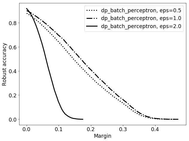
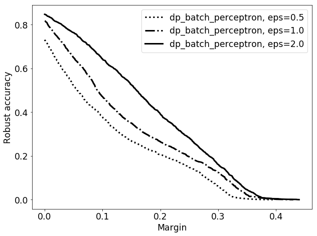
As for noise addition, the robustness guarantee for such kernel classifiers is also more complicated than the non-kernel linear classifiers. In Section G.2.1 below, we provide a provable robustness guarantee of the kernel classifiers. Using this provable guarantee, the empirical robustness accuracy is shown in the last column of Figure 4 and its comparison to DP-SGD-trained CNNs is shown in Figure 5. Even though the kernel classifiers start off with similar accuracy (at $\gamma=0$ ), it quickly drops and becomes worse than CNNs. We remark here that, in addition to the nature of the kernel, this may also be exacerbated by the fact that the provable robust guarantee for the kernel classifiers is not tight (unlike the non-kernel case).

G.2.1 Robustness Guarantee for Multi-Class Perceptron with Kernel

To compute the robust error for the kernel classifiers, we will use the following result, which is a slightly simplified version of Theorem 2.1 from (Hein and Andriushchenko 2017).

Lemma 22.

Let $M$ be a classifier which, for each class $y\in\{1,\dots,k\}$ , computes some function $f^{y}:\mathbb{R}^{d}\to\mathbb{R}$ and predicts the class $y^{*}$ that minimizes $f^{y^{*}}$ . Then, for every example $(\mathbf{x},y)$ and any $\Delta\in\mathbb{R}^{d}$ such that

\displaystyle\|\Delta\|\leq\min_{y^{\prime}\neq y}\frac{f^{y}(\mathbf{x})-f^{y^{\prime}}(\mathbf{x})}{\sup_{\mathbf{x}^{\prime}\in\mathbb{R}^{d}}\|\nabla f^{y}(\mathbf{x}^{\prime})-\nabla f^{y^{\prime}}(\mathbf{x}^{\prime})\|},

the classifier $M$ predicts $y$ on $\mathbf{x}+\Delta$ .

Note that this lemma is tight for the non-kernel case, leading to the margin formula $\gamma<\min_{y^{\prime}\neq y}\frac{\left<\mathbf{w}^{(y)},\mathbf{x}\right>-\left<\mathbf{w}^{(y^{\prime})},\mathbf{x}\right>}{\|\mathbf{w}^{(y)}-\mathbf{w}^{(y^{\prime})}\|}$ that we used earlier.

Our kernel classifier is of the form in Lemma 22 with $f^{y}(\mathbf{x}^{\prime}):=\left<\mathbf{w}^{(y)},\phi_{\rho_{1},\dots,\rho_{\hat{d}}}(\mathbf{x}^{\prime})\right>$ . To apply the lemma, we first compute $\nabla f$ :

\displaystyle\nabla f^{y}(\mathbf{x}^{\prime})=\frac{1}{\sqrt{\hat{d}}}\cdot\sum_{i=1}^{\hat{d}}\left(-w^{(y)}_{i}\cdot\sin(\left<\rho_{i},\mathbf{x}^{\prime}\right>)+w^{(y)}_{\hat{d}+i}\cdot\cos(\left<\rho_{i},\mathbf{x}^{\prime}\right>)\right)\cdot\rho_{i}.

As a result, for two classes $y,y^{\prime}$ , we have

\displaystyle\nabla f^{y}(\mathbf{x}^{\prime})-\nabla f^{y^{\prime}}(\mathbf{x}^{\prime})=\frac{1}{\sqrt{\hat{d}}}\cdot\sum_{i=1}^{\hat{d}}\left((w^{(y^{\prime})}_{i}-w^{(y)}_{i})\cdot\sin(\left<\rho_{i},\mathbf{x}^{\prime}\right>)+(w^{(y)}_{\hat{d}+i}-w^{(y^{\prime})}_{\hat{d}+i})\cdot\cos(\left<\rho_{i},\mathbf{x}^{\prime}\right>)\right)\cdot\rho_{i}.

In the following, we will give an upper bound on $\|\nabla f^{y}-\nabla f^{y^{\prime}}\|$ . Let $\Pi\in\mathbb{R}^{d\times\hat{d}}$ resulting from concatenating $\rho_{1},\dots,\rho_{\hat{d}}$ , and let $\mathbf{p}\in\mathbb{R}^{\hat{d}}$ denote the vector for which $p_{i}=\frac{1}{\sqrt{\hat{d}}}(w^{y^{\prime}}_{i}-w^{y}_{i})\cdot\sin(\left<\rho_{i},\mathbf{x}^{\prime}\right>)+(w^{y}_{\hat{d}+i}-w^{y^{\prime}}_{\hat{d}+i})\cdot\cos(\left<\rho_{i},\mathbf{x}^{\prime}\right>)$ . First, notice that

\displaystyle\nabla f^{y}-\nabla f^{y^{\prime}}=\Pi\mathbf{p}.

Now, we may bound $\|\mathbf{p}\|$ by

	$\displaystyle\\|\mathbf{p}\\|$	$\displaystyle=\frac{1}{\sqrt{\hat{d}}}\cdot\sqrt{\sum_{i=1}^{\hat{d}}\left((w^{(y^{\prime})}_{i}-w^{(y)}_{i})\cdot\sin(\left<\rho_{i},\mathbf{x}^{\prime}\right>)+(w^{(y)}_{\hat{d}+i}-w^{(y^{\prime})}_{\hat{d}+i})\cdot\cos(\left<\rho_{i},\mathbf{x}^{\prime}\right>)\right)^{2}}$
	$\displaystyle(\text{Cauchy\textendash Schwarz inequality})$	$\displaystyle\leq\frac{1}{\sqrt{\hat{d}}}\cdot\sqrt{\sum_{i=1}^{\hat{d}}\left((w^{(y^{\prime})}_{i}-w^{(y)}_{i})^{2}+(w^{(y)}_{\hat{d}+i}-w^{(y^{\prime})}_{\hat{d}+i})^{2}\right)\left(\sin(\left<\rho_{i},\mathbf{x}^{\prime}\right>)^{2}+\cos(\left<\rho_{i},\mathbf{x}^{\prime}\right>)^{2}\right)}$
		$\displaystyle=\frac{1}{\sqrt{\hat{d}}}\cdot\sqrt{\sum_{i=1}^{\hat{d}}\left((w^{(y^{\prime})}_{i}-w^{(y)}_{i})^{2}+(w^{(y)}_{\hat{d}+i}-w^{(y^{\prime})}_{\hat{d}+i})^{2}\right)}$
		$\displaystyle=\frac{1}{\sqrt{\hat{d}}}\cdot\\|\mathbf{w}^{(y)}-\mathbf{w}^{(y^{\prime})}\\|$

As a result, we have

\displaystyle\|\nabla f^{y}(\mathbf{x}^{\prime})-\nabla f^{y^{\prime}}(\mathbf{x}^{\prime})\|=\|\Pi\mathbf{p}\|\leq\sigma_{\max}(\Pi)\cdot\frac{1}{\sqrt{\hat{d}}}\cdot\|\mathbf{w}^{(y)}-\mathbf{w}^{(y^{\prime})}\|,

where $\sigma_{\max}(\Pi)$ denote the largest singular value of $\Pi$ (i.e. the operator norm of $\Pi$ with respect to $L_{2}$ norm).

Plugging this back into Lemma 22, we can conclude that each example $(\mathbf{x},y)$ remaining correctly classifies up to perturbation norm of

\displaystyle\frac{\sqrt{\hat{d}}}{\sigma_{\max}(\Pi)}\cdot\min_{y^{\prime}\neq y}\frac{f^{y}(\mathbf{x})-f^{y^{\prime}}(\mathbf{x})}{\|\mathbf{w}^{(y)}-\mathbf{w}^{(y^{\prime})}\|}.

G.3 Comparison with Support Vector Machines (SVM)

Previous work has introduced different approaches to preserving DP for SVM (Rubinstein et al. 2012), or convex optimization algorithms in general (Feldman et al. 2020; Bassily et al. 2019). Our implementation of DP SVM uses DP SGD (Abadi et al. 2016) with the standard hinge loss and $L_{2}$ weight regularization. The regularization strength is chosen from 1, 0.1, 0.01, 0.001, 0.0001, 0.00001, the learning rate from 1, 0.1, 0.01, 0.001, 0.0001. After summing gradients from each batch of data, we add appropriately calibrated Gaussian noise (again, based on Renyi DP) to the weights update.

Figures 6 and 7 compare performance of DP Batch Perceptron and DP SVM with and without kernel respectively. For experiments with varying $\epsilon$ (first column in both figures), we observe that DP Batch Perceptron outperforms DP SVM in most instances and achieves competitive accuracy on both datasets. For different $\delta$ values (second column) while keeping $\epsilon$ fixed at 1.0, the trend still holds to a large extent and both algorithms yield very similar test accuracy. The last column compares the robust accuracy of models trained via DP Batch Perceptron and DP SVM at $\epsilon=1,2$ . In the case where no kernel is involved, the former yields better results on MNIST dataset but performs worse on USPS dataset. The opposite trend is observed when Gaussian kernel is included.

	$\displaystyle\mathbb{E}_{\mathbf{q}\sim\mathcal{U}_{[0,1]}^{\otimes d},\mathbf{w}\sim\mathbb{B}_{\tilde{\mathcal{P}}_{\mathbf{q}}}}[\\|\mathbf{w}\\|^{2}]$	$\displaystyle=\mathbb{E}_{\mathbf{q}_{1},\dots,\mathbf{q}_{T^{2}},\mathbf{q}\sim\mathcal{U}_{[0,1]}^{\otimes d},i^{}\sim[T],\mathbf{w}\sim\mathbb{A}(\tilde{\mathcal{Q}}^{n})}\left[\\|T\cdot\mathbf{w}^{i^{}}\\|^{2}\right]$
		$\displaystyle=\mathbb{E}_{\mathbf{q}_{1},\dots,\mathbf{q}_{T^{2}}\sim\mathcal{U}_{[0,1]}^{\otimes d},i^{}\sim[T],\mathbf{w}\sim\mathbb{A}(\mathcal{Q}^{n})}\left[\\|T\cdot\mathbf{w}^{i^{}}\\|^{2}\right]$
		$\displaystyle=\mathbb{E}_{\mathbf{q}_{1},\dots,\mathbf{q}_{T^{2}}\sim\mathcal{U}_{[0,1]}^{\otimes d},\mathbf{w}\sim\mathbb{A}(\mathcal{Q}^{n})}\left[\frac{1}{T^{2}}\cdot\sum_{i^{}\in[T^{2}]}\\|T\cdot\mathbf{w}^{i^{}}\\|^{2}\right]$
		$\displaystyle=\mathbb{E}_{\mathbf{q}_{1},\dots,\mathbf{q}_{T^{2}}\sim\mathcal{U}_{[0,1]}^{\otimes d},\mathbf{w}\sim\mathbb{A}(\mathcal{Q}^{n})}\left[\\|\mathbf{w}\\|^{2}\right]$
		$\displaystyle\leq 1.$

	$\displaystyle\mathbb{E}_{\mathbf{q}\sim\mathcal{U}_{[0,1]}^{\otimes d},\mathbf{w}\sim\mathbb{B}_{\tilde{\mathcal{P}}_{\mathbf{q}}}}[\err^{\tilde{\mathcal{P}}_{\mathbf{q}}}_{\gamma_{0}}(\mathbf{w})]$	$\displaystyle=\mathbb{E}_{\mathbf{q}_{1},\dots,\mathbf{q}_{T^{2}},\mathbf{q},i^{},\mathbf{w}\sim\mathbb{A}(\tilde{\mathcal{Q}}^{n})}\left[\err^{\tilde{\mathcal{P}}_{\mathbf{q}}}_{\gamma_{0}}(T\cdot\mathbf{w}^{i^{}})\right]$
		$\displaystyle=\mathbb{E}_{\mathbf{q}_{1},\dots,\mathbf{q}_{T^{2}},i^{},\mathbf{w}\sim\mathbb{A}(\mathcal{Q}^{n})}\left[\err^{\tilde{\mathcal{P}}_{\mathbf{q}}}_{\gamma_{0}/T}(\mathbf{w}^{i^{}})\right]$
	$\displaystyle(\text{Since }\gamma_{0}/T\leq 0.1\gamma)$	$\displaystyle\leq\mathbb{E}_{\mathbf{q}_{1},\dots,\mathbf{q}_{T^{2}},i^{},\mathbf{w}\sim\mathbb{A}(\mathcal{Q}^{n})}\left[\err^{\mathcal{P}_{\mathbf{q}}}_{0.1\gamma}(\mathbf{w}^{i^{}})\right]$
		$\displaystyle=\mathbb{E}_{\mathbf{q}_{1},\dots,\mathbf{q}_{T^{2}},\mathbf{w}\sim\mathbb{A}(\mathcal{Q}^{n})}\left[\frac{1}{T^{2}}\sum_{i^{}\in[T^{2}]}\err^{\tilde{\mathcal{P}}_{\mathbf{q}}}_{0.1\gamma}(\mathbf{w}^{i^{}})\right]$
		$\displaystyle=\mathbb{E}_{\mathbf{q}_{1},\dots,\mathbf{q}_{T^{2}},\mathbf{w}\sim\mathbb{A}(\mathcal{Q}^{n})}\left[\err^{\mathcal{Q}}_{0.1\gamma}(\mathbf{w})\right].$

$\displaystyle\\|\mathbf{w}_{i}\\|^{2}$	$\displaystyle=\\|\mathbf{w}_{i-1}+\mathbf{u}_{i}+\mathbf{g}_{i}\\|^{2}$
	$\displaystyle=\\|\mathbf{w}_{i-1}+\mathbf{u}_{i}\\|^{2}+2\left<\mathbf{w}_{i-1}+\mathbf{u}_{i},\mathbf{g}_{i}\right>+\\|\mathbf{g}_{i}\\|^{2}$
$\displaystyle(\text{From }E_{\text{parallel}})$	$\displaystyle\leq\\|\mathbf{w}_{i-1}+\mathbf{u}_{i}\\|^{2}+0.02\alpha\gamma_{\text{gap}}B\cdot\\|\mathbf{w}_{i-1}+\mathbf{u}_{i}\\|+\\|\mathbf{g}_{i}\\|^{2}$
$\displaystyle(\text{From }E_{\text{noise-norm}})$	$\displaystyle\leq\\|\mathbf{w}_{i-1}+\mathbf{u}_{i}\\|^{2}+0.02\alpha\gamma_{\text{gap}}B\cdot\\|\mathbf{w}_{i-1}+\mathbf{u}_{i}\\|+\alpha B^{2}$
	$\displaystyle\leq\\|\mathbf{w}_{i-1}\\|^{2}+2\left<\mathbf{w}_{i-1},\mathbf{u}_{i}\right>+\\|\mathbf{u}_{i}\\|^{2}+0.02\alpha\gamma_{\text{gap}}B\cdot\left(\\|\mathbf{w}_{i-1}\\|+\\|\mathbf{u}_{i}\\|\right)+\alpha B^{2}$	(13)

	$\displaystyle\\|\mathbf{w}_{i}\\|^{2}$	$\displaystyle\leq\\|\mathbf{w}_{i-1}\\|^{2}+\left(2\|M_{i}\|\gamma^{\prime}+0.02\alpha\gamma_{\text{gap}}B\right)\cdot\\|\mathbf{w}_{i-1}\\|+(\|M_{i}\|^{2}+0.02\alpha\gamma_{\text{gap}}B\|M_{i}\|+\alpha B^{2})$
		$\displaystyle\leq\\|\mathbf{w}_{i-1}\\|^{2}+\left(2\|M_{i}\|\gamma^{\prime}+0.02\alpha\gamma_{\text{gap}}B\right)\cdot\\|\mathbf{w}_{i-1}\\|+(\|M_{i}\|^{2}+0.02B\cdot\|M_{i}\|+\alpha B^{2})$
		$\displaystyle\leq\\|\mathbf{w}_{i-1}\\|^{2}+\left(2\|M_{i}\|\gamma^{\prime}+0.02\alpha\gamma_{\text{gap}}B\right)\cdot\\|\mathbf{w}_{i-1}\\|+2B\|M_{i}\|+\alpha B^{2},$

Abstract

1 Introduction

Background.

Definition 1 (Differential Privacy (DP) (Dwork et al. 2006b; Dwork et al. 2006a)).

Our Results.

Theorem 2.

Theorem 3.

Theorem 4.

Theorem 5.

Theorem 6.

Organization.

2 Sample Complexity Lower Bounds

2.1 Pure-DP Lower Bound (Theorem 2)

2.2 Approximate-DP Lower Bound (Theorem 3)

2.3 Non-Robust DP Learning Lower Bound (Theorem 4)

3 Sample-Efficient Algorithms

3.1 Pure-DP Algorithm (Theorem 5)

3.2 Approximate-DP Algorithm (Theorem 6)

4 Experiments

Adversarial Robustness Evaluation.

5 Other Related Work

Learning Halfspaces with Margin.

Adversarially Robust Learning.

Differentially Private Learning.

6 Conclusions and Future Directions

References

Appendix A Preliminaries

A.1 Margin of Halfspaces

Lemma 7.

A.2 Boosting the Success Probability

Observation 8.

Proof Sketch.

Appendix B Lower Bound for Robust Learning of Halfspaces: Pure-DP Case

Lemma 9.

Proof of Theorem 2.

Claim 10.

Proof.

Proof of Lemma 9.

Appendix C Lower Bound for Robust Learning of Halfspaces: Approximate-DP Case

Theorem 11 ((Steinke and Ullman 2017, Theorem 3)).

C.1 Lower Bound for γ=Ω⁡(1)\gamma=\Omega(1)

Lemma 12.

Proof.

Lemma 13.

Proof.

C.2 Lower Bound for Smaller γ\gamma

Lemma 14.

Proof.

Proof.

Appendix D Lower Bound for Non-Robust Learning of Halfspaces

Lemma 15.

Proof.

Proof of Theorem 4.

Appendix E Pure DP Robust Learner

Lemma 16 (Generalization Bound for Large Margin Halfspaces (Bartlett and Mendelson 2002)).

Proof of Theorem 5.

Lemma 17.

Appendix F Approximate-DP Robust Learner

F.1 Utility Analysis

Lemma 18.

Proof.

F.2 Privacy Analysis

Lemma 19.

Lemma 20 (Amplification by Subsampling (Balle et al. 2018)).

Lemma 21 (Advanced Composition (Dwork et al. 2010)).

Proof of Lemma 19.

F.3 Putting Things Together

Proof of Theorem 6.

Appendix G Additional Experiments

G.1 Adversarial Robustness Evaluation on USPS Dataset

G.2 Experiments with Gaussian Kernel

G.2.1 Robustness Guarantee for Multi-Class Perceptron with Kernel

Lemma 22.

G.3 Comparison with Support Vector Machines (SVM)

C.1 Lower Bound for $\gamma=\Omega(1)$

C.2 Lower Bound for Smaller $\gamma$